2021 Economic Impact Analysis Emissions Pathway Review

with

2021 Economic Impact Analysis – Emissions Pathway Review Final report

Prepared for:

The Tasmanian Government

Page 2 of 35

CONTENTS

About the authors of this report .................................................................................................................................... 3

Victoria University ................................................................................................................................................................ 3

Centre of Policy Studies ................................................................................................................................................... 3 Recent work on greenhouse gas issues in Australia ........................................................................................................ 3 Philip Adams .................................................................................................................................................................... 4

Point Advisory ....................................................................................................................................................................... 4

1 Executive summary ............................................................................................................................................. 5

1.1 Context ...................................................................................................................................................................... 5

1.2 Project background ................................................................................................................................................... 5

1.3 Economic impacts of the best-fit emissions reduction pathway ............................................................................... 5

2 Introduction ........................................................................................................................................................ 7

2.1 Context ...................................................................................................................................................................... 7

2.2 Objectives of this project ........................................................................................................................................... 7

2.3 Linkages with 2021 TEPR project ............................................................................................................................... 7

2.4 Structure of this report .............................................................................................................................................. 8

2.5 Limitations ................................................................................................................................................................. 8

3 Methodology .................................................................................................................................................... 10

3.1 Model and reference year database ....................................................................................................................... 10

3.2 Basecase projection ................................................................................................................................................. 10

3.3 Inputs for modelling-best fit emissions scenario..................................................................................................... 11

3.3.1 Exogenous shocks: Stationary energy ............................................................................................................. 11 3.3.2 Exogenous shocks: Transport fuel ................................................................................................................... 12 3.3.3 Exogenous shocks: Industrial .......................................................................................................................... 12 3.3.4 Exogenous shocks: Agriculture ........................................................................................................................ 12 3.3.5 Exogenous shocks: LULUCF ............................................................................................................................. 12 3.3.6 Exogenous shocks: Waste ............................................................................................................................... 12

3.4 Simulation design .................................................................................................................................................... 15

3.4.1 Labour markets ............................................................................................................................................... 15 3.4.2 Private consumption and investment ............................................................................................................. 15 3.4.3 Government consumption and fiscal balances ............................................................................................... 15 3.4.4 Production technologies and household tastes .............................................................................................. 15

4 Results and analysis .......................................................................................................................................... 16

4.1 Economic impacts .................................................................................................................................................... 16

4.1.1 Real GSP .......................................................................................................................................................... 16 4.1.2 Tasmanian employment ................................................................................................................................. 17 4.1.3 Tasmanian industry output ............................................................................................................................. 17 4.1.4 Tasmanian industry employment ................................................................................................................... 20

4.2 Conclusions .............................................................................................................................................................. 20

Appendix 1 Additional VURM information .............................................................................................................. 22

Appendix 2 Equations used to understand VURM GSP calculations ......................................................................... 22

Appendix 3 Detailed industry results ....................................................................................................................... 23

Appendix 4 Emissions reduction impacts of best-fit opportunities .......................................................................... 34

Page 3 of 35

ABOUT THE AUTHORS OF THIS REPORT

Our project team consists of Professor Philip Adams from the Centre of Policy Studies, Victoria University and Point Advisory, an integrated sustainability consultancy.

Victoria University

Centre of Policy Studies

The Centre of Policy Studies (CoPS) is a research centre located at Victoria University, Melbourne1. CoPS specialises in Computable General Equilibrium (CGE) modelling. It undertakes academic/contract research and software development, conducts training courses in CGE modelling and offers graduate student supervision. CoPS has around 20 academic staff employed full time at the Centre, including 7 full professors and 3 associated professors.

CoPS’ suite of Australian models includes several detailed, dynamic CGE models of Australia, which have been used to analyse many economic policies, including changes in taxes, tariffs, environmental regulations and competition policy. CoPS’ In recent years, CoPS has developed and applied national economic models to assess the impact of economic changes in many other countries and has developed its own version of the global GTAP model. CoPS’ modelling work is facilitated by the use of computer software developed at the Centre. This software, known as GEMPACK, is used in about 700 different locations around the world.

Recent work on greenhouse gas issues in Australia

CoPS involvement in greenhouse issues began in 1991 with its modelling for the Australian government of issues associated with the Environmental Sustainable Development (ESD) process. Since then, it has provided model-based advice to numerous government-based policy processes. For example, CoPS’ modelling lays at the heart of the analytics underlying Garnaut’s Climate Change Review and the Federal Treasury’s two studies on emissions policy, one published in late 2008 and dealing with the Federal plan for a Carbon Pollution Reduction Scheme, the other published in 2011 and dealing with the Clean Energy Future.

Applications of CoPS’ models (particularly the Victoria University Regional Model (VURM)) have been central to many consultancy reports examining greenhouse issues in Australia, including (recently):

“Upside and Downside Risks of Climate Change” for the NSW Treasury (Philip Adams) (2020-21).

“Covid-19, Energy and Climate Change” for the Department of Industry, Science, Energy and Resources” with Frontier Economics (Philip Adams) (2020-21).

“Impacts of the National Energy Guarantee with specific reference to Victorian industries and Regions”, for the Department of Environment, Land, Water and Planning (Victoria) (Philip Adams) (2018).

Simulations and Analysis of Options for Queensland’s Renewable Energy Expert Panel2 (Philip Adams) (2016).

“Economic Impacts of Various Aspects of the Nuclear Fuel Cycle”, for the Nuclear Fuel Cycle Royal Commission in South Australia with Ernst and Young (Philip Adams) (2015-16).

“Australia is ‘free to choose’ Economic Growth and Falling Environmental Pressures”, inputs to a wider CSIRO study on energy futures. Summary published in Nature, Vol. 527, November 2015, 49-53.

“Australian National Outlook 2015 and 2017: Economic Activity, Resource Use, Environmental Performance and Living Standards, 1970-2050”, for CSIRO, Canberra (Philip Adams) (2011-2017).

“Pathways to Deep Decarbonisation in 2050: How Australia Can Prosper in a Low Carbon World” for ClimateWorks Australia (Philip Adams) (2014-2016)3.

For a general description of applications like those described above, see:

Philip D. Adams and Brian R. Parmenter, “Computable General Equilibrium Modelling of Environmental issues in Australia: Economic Impacts of an Emissions Trading Scheme” in P.B. Dixon and D. Jorgenson (eds) Handbook of CGE Modelling, Vol. 1A, 2013, Elsevier B.V.

–

1 http://www.copsmodels.com/

2 https://www.dews.qld.gov.au/electricity/solar/solar-future/expert-panel

3 http://climateworks.com.au/project/national-projects/pathways-deep-decarbonisation-2050-how-australia-can-prosper-low-carbon

http://www.copsmodels.com/

https://www.dews.qld.gov.au/electricity/solar/solar-future/expert-panel

http://climateworks.com.au/project/national-projects/pathways-deep-decarbonisation-2050-how-australia-can-prosper-low-carbon

Page 4 of 35

Philip Adams

Philip is Professor at the Centre of Policy Studies (CoPS), Victoria University, Melbourne. Prior to his current position, Philip was Director and Professor at CoPS, Monash University (2004-2013). Philip was elected a Fellow of the Academy of the Social Sciences in Australia in 2016. In that year, he was also awarded the GTAP Research Fellow distinction for the term of 2016 to 2019.

Philip's main area of expertise is the application of large multi-sectoral and multi-regional economic models for policy analysis and forecasting. Since completing his Ph.D., he has been involved in the implementation of several large models of the Australian economy and has been active in developing models for overseas organisations, including central government organisations in Saudi Arabia, Oman, Jordan, Uganda, South Africa, Taiwan, Denmark, and Thailand.

Philip’s work has focussed on a range of areas, including the economics of climate change, climate change adaptation and climate change mitigation. Clients include: the Garnaut Climate Change Review, the Federal Treasury, the state treasuries of VIC, NSW, QLD and WA, the Commonwealth Scientific and Industrial Research Organisation (CSIRO), the DCCEE, Climate Works, Climate Institute and the WWF. His technical advice for the Federal Treasury led to the adoption of the MMRF system as Treasury’s principal tool for analysis greenhouse mitigation policies from 2006 through to the present day. More recently he has worked: as technical advisor for Australia’s participation in the global 2050 Deep Decarbonisation Pathways Project (DDPP), coordinated by the Sustainable Development Solutions Network (SDSN)4; for the International Policy Division of the Department of Foreign Affairs (Climate change and sustainability branch) on a fact-finding mission to India (June 2013) designed to find potential partners for a joint Australia/India study on climate change issues; and with the CSIRO on a number of projects, including the development of a large scale, detailed Integrated Assessment Model (IAM), and simulations for the Australian National Outlook (leading to a publication in Nature).

Point Advisory

Point Advisory is an integrated sustainability consultancy providing specialist technical, strategic and assurance services the following domains:

• Climate change mitigation, adaptation and assurance

• Energy efficiency, renewable energy and energy analytics

• Environmental management, compliance, air quality and audit

• Environmental economics, program evaluation and natural capital

• Green buildings and infrastructure

• Sustainability policy and analysis.

Since 2013, we have provided these services to clients from all levels of government, the corporate sector and not-for-profits. We specialise in combining our technical engineering skills with economic and strategic capabilities to develop robust, viable and effective solutions for our clients.

Our team has had extensive experience developing net zero strategies for both state and local governments, and has worked closely with the Tasmanian Government on its net zero emissions strategy since 2018.

– 4 http://www.climateworksaustralia.org/project/current-project/pathways-deep-decarbonisation-2050-how-australia-can-prosper-low-carbon

https://pointadvisory.com/?gclid=Cj0KCQjw8vqGBhC_ARIsADMSd1AYyo3dGCy5Pa1TPT6fF7zAT_sChLGRAEgm2J7mK4YmD7tJOcsPUh0aAr7rEALw_wcB

http://www.climateworksaustralia.org/project/current-project/pathways-deep-decarbonisation-2050-how-australia-can-prosper-low-carbon

Page 5 of 35

1 EXECUTIVE SUMMARY

1.1 Context

There is now overwhelming evidence that our climate is changing as a result of human-induced emissions of greenhouse gases. The resulting rising temperatures will have a significant impact on rainfall, evaporation and sea level, among many other things. These changes are likely to make our climate more variable and result in more frequent and severe extreme weather events.

To address this situation, in 2015, countries from around the world signed up to the Paris Agreement. This commits countries to keeping global temperature rise to well below 2 degrees Celsius, and to make every effort to keep them below 1.5 degrees Celsius, compared to pre-industrial levels. In practical terms, this means that greenhouse gas emissions need to peak now and reach net zero by 2050 at the latest. The Paris Agreement recognises the important role of sub-national governments in responding to climate change, however meeting this challenge is a shared responsibility that will require action from communities, businesses and governments from around the world.

At the domestic level, all states and territories in Australia now have some form of net zero commitment by 2050. Most notably, Victoria has a legislated target to achieve net zero emissions by 2050, and the ACT has a net zero target by 2045. At the international level, a number of countries have set net zero emissons targets by 2050 (or earlier), including many that are enshrined in law. At the federal level, although no firm target has been set, the Prime Minister, Scott Morrison, has affirmed the need for Australia to achieve net zero emissions by 2050, if possible.

1.2 Project background

With its significant forest estate and low carbon electricity sector, Tasmania is well placed amongst Australian states and territories to achieve net zero emissions at a relatively low cost. Our analysis indicates that Tasmania could achieve and maintain net zero emissions much earlier than 2050, whilst continuing to grow the state’s economy. In fact, if all identified emissions reduction opportunities were implemented, Tasmania would maintain net zero emissions from now onwards.

Under Tasmania’s existing Climate Change (State Action) Act 2008 (the Act), the state passed a legally binding target to reduce emissions by at least 60% below 1990 levels by 2050. Through the subsequent release of Climate Action 21, the Tasmanian Government has committed to a target of net zero emissions by 2050. As part of the independent review of the Act, the Tasmanian Government is seeking to set a more ambitious emissions reduction target for Tasmania, aligned with the goals of the Paris Agreement.

To assist with this process, the Tasmanian Government has undertaken a 2021 update of Tasmania’s Emissions Pathway Review (TEPR), building on the analysis undertaken as part of the 2019 review project. This work has been delivered by Point Advisory and forestry specialists Indufor. This project developed a best-fit emissions reduction pathway for Tasmania, comprised of 16 emissions reduction opportunities, that, if implemented, would mean Tasmania would maintain net zero emissions status from now until 2050.

To understand the economic impacts of implementing this best-fit emissions reduction pathway, the Tasmanian Government commissioned Victorian University and Point Advisory to undertake a detailed economic analysis of this pathway, using computable general equilibrium (CGE) modelling.

It should be noted that the objective of CGE modelling is to estimate the overall impact of the best-fit emissions reduction pathway on the Tasmanian economy, not to provide a benefit-cost analysis of initiatives or actions necessary to achieve it. Action planning and resourcing will have to be refined by the Tasmanian government iteratively over the period.

1.3 Economic impacts of the best-fit emissions reduction pathway

Bottom-up CGE modelling was undertaken using the Victoria University Regional Model (VURM) to analyse the impact of the best-fit emissions reduction pathway on Tasmania’s economy to 2050. VURM has been used extensively for modelling climate change policies, and issues associated with climate change and adaptation.

The analysis showed that the transition to a net zero carbon economy could deliver economic benefits across all sectors of the Tasmanian economy, including an increase in real Gross State Product (GSP) relative to a basecase

Page 6 of 35

simulation by 0.19%, or just over $67 million in 2030, and $475 million in 2050 (0.92%), both 2021 prices. In addition, employment could be up (relative to basecase) by 0.14% by 2030, or 145 persons employed, and 1,260 persons employed by 2050 (0.47% increase).

The greater contributing sector, in terms of output and employment, is agriculture, forestry and fishing, contributing more than 50% to the overall increase in real GSP across Tasmania. In 2050, relative to basecase levels, real value added in the sheep (including lamb) and cattle (beef plus dairy) industries could expand by around $70 million, while real value added in Forestry and Logging could be up $55 million. It must be noted that these benefits are, to a large extent, due to productivity gains expected to result from adoption of technology uptake, and increased plantation activity on already established plantation land, or marginal agricultural land, rather than any increase in native forest harvesting rates or animal numbers (relative to the basecase).

Other important sectors include manufacturing, which expands, relative to its basecase level, by 0.1%, or $1.8m (2021 prices) by 2030, and by 0.4%, or $13.5m (2021 prices) by 2050. Production of construction services rises (compared to basecase) by 0.4%, or $8m (2021 prices) by 2030, and by 0.7%, or $20.5m (2021 prices) by 2050, while collectively ANZSIC Divisions F to T (see Appendix 3) expand by $26.5m (2021 prices) by 2030, and by $123.5m by 2050.

Importantly, under the assumptions made, no ANZSC division would lose significant employment due to the deployment of the best-fit emissions reduction opportunities modelled, although there may be some reallocation within sectors in favor of less emission intensive production processes.

Page 7 of 35

2 INTRODUCTION

2.1 Context

Under Tasmania’s existing Climate Change (State Action) Act 2008 (the Act), the state passed a legally binding target to reduce emissions by at least 60% below 1990 levels by 2050. Through the subsequent release of Climate Action 21, the Tasmanian Government committed to a target of net zero emissions by 2050. As part of the independent review of the Act, the Tasmanian Government is seeking to set a more ambitious emissions reduction target for Tasmania, aligned with the goals of the Paris Agreement.

In the State of the State Address in March 20205, the Premier requested that the Tasmanian Government “conduct a detailed analysis of the pathway our state would need to take and the impacts on industry and jobs to achieve a target of zero net emissions prior to 2050”.

Three key projects were commissioned to support the above commitments:

Independent review of the Climate Change (State Action) Act 2008: Consult with business, industry, local government and the broader community about the options for setting a more ambitious net zero emissions reduction target for Tasmania, as part of the consultation process for the independent review of the Climate Change (State Action) Act conducted by consulting firm Jacobs.

Tasmanian Emissions Pathway Review: Undertake a 2021 update of Tasmania’s Emissions Pathway Review (TEPR), building on the analysis undertaken as part of the 2019 review project. This work has been delivered by Point Advisory and Indufor.

Economic Impact Analysis: Undertake a detailed economic analysis of potential emissions reduction targets, using computable general equilibrium (CGE) modelling of the impact on Tasmania' s economy and employment of potential emissions pathways. This work has been delivered by Victoria University and Point Advisory.

This report details the analysis related to the Economic Impact Analysis project.

2.2 Objectives of this project

The overall objectives of this project were to provide CGE economic analysis of the best-fit emissions reduction pathway for Tasmania, as defined in the separate “2021 Update of Tasmania’s Emissions Pathways Review” project (TEPR 2021 project).

2.3 Linkages with 2021 TEPR project

The scenarios used in the CGE model have been built using the assumptions made in the 2021 TEPR project. Table 1 below outlines how these two projects link in terms of scenario development.

Table 1. Linkages in scenario development between 2021 TEPR and this project

Scenario TEPR project CGE model

Business as usual scenario

Medium reference case emissions trajectory

Base Case economic projections to 2050

Emissions reductions pathway scenario

Best-fit emissions reduction pathway with 16 opportunities modelled

Best-fit emissions scenario: Economic projections to 2050 presented as a deviation to the Base Case, taking into account the economic impacts of the opportunities quantified.

Appendix 4 identifies the 16 best fit emissions reduction opportunities and how they are described across both projects.

– 5 http://www.premier.tas.gov.au/releases/state_of_the_the_state_address

http://www.premier.tas.gov.au/releases/state_of_the_the_state_address

Page 8 of 35

2.4 Structure of this report

This report is structured as follows:

Section 3: This section provides an overview of the methodology used for the CGE modelling.

Section 4: This section provides the results of the CGE modelling showing the impact of the roll-out of the best-fit emissions opportunities on Tasmania’s Real GSP, overall and industry specific employment, and industry output.

Appendix 1: This provides additional information on the Victoria University Regional Model (VURM) used for the CGE analysis.

Appendix 2: This provides the equations used to understand the VURM GSP calculations.

Appendix 3: This provides tables detailing the CGE modelling results.

Appendix 4: This provides the emissions reduction impacts of the best-fit opportunities included in the economic modelling.

2.5 Limitations

It should be noted that the transition to a low-emissions economy for any state will be uncertain and take time. The following points outline the limitations associated with the analysis:

The purpose of CGE modelling is to estimate the overall impact of the best-fit emissions reduction pathway on the Tasmanian economy, not to provide a benefit-cost analysis of initiatives or actions necessary to achieve it and to assess different implementation actions.

− CGE modelling offers limited guidance on the impacts of policy suites, because the dynamic and inter-connected modelling character of CGE modelling makes is impossible to disintegrate the effect of various assumptions (unless different scenarios are created).

− As such, quantifying and analysing the economic viability of each discrete opportunity (for example by calculating a Net Present Value for each option) identified in the emissions pathway review was not in the scope of the engagement.

− Identifying the funding needs specifically for Government across these opportunities was outside the scope of this engagement. Planning and resourcing to achieve the desired net benefit will need to be undertaken by the Tasmanian government iteratively over the period.

The CGE modelling does not assess the climate damages associated with Tasmania not taking climate action in line with the best-fit emissions scenario, as Tasmania’s emission trajectory will have no impact on overall global warming and hence there will be no differentiated damage costs related to different State-specific emissions reduction trajectories.

The cost e.g. level of investment, and benefits e.g. efficiency gains, for each modelled opportunity identified by Point Advisory and used by Victoria University as inputs to the VURM model are based on information gathered through both the 2018/19 Tasmanian Emissions Pathway Review (TEPR) project and new resources (where available) and is valid at a specific point in time and within the boundaries of the assessment. These costs and benefits are explained in detail in Appendix 2 of the separate 2021 update of the TEPR report.

Sectoral aspects

It is acknowledged that the costs and benefits for opportunities within the manufacturing sector will be highly site-, process- and fuel-specific, and payback periods will vary significantly, depending on world markets and speed of innovation and adoption of innovation, not only in Tasmania or Australia, but also worldwide.

Although considered as part of the TEPR best-fit emissions scenario, the economic impacts of hydrogen were not included as part of the CGE modelling for the following reasons:

− Renewable hydrogen represents a new industry that is not represented in the CGE model used for this analysis.

− Only the domestic part of the hydrogen “business case” is included in the best-fit emissions scenario, which is simply the most likely first step in the development of the hydrogen value chain in Tasmania. Therefore, considering only domestic hydrogen production and use in the short to medium term would likely underestimate long term benefits that would arise from being part of a growing export market, assuming that it develops as expected. Producing renewable hydrogen for exports is not considered as part of the

Page 9 of 35

emissions trajectory, as the production is likely to be very low emissions and will only marginally impacts Tasmanian’s domestic emissions (contrary to domestic use).

− The Tasmanian Government is already separately exploring the opportunities for developing a Renewable Hydrogen industry via the Tasmanian Renewable Hydrogen Action Plan, which sets out a vision for Tasmanian to capitalise on its existing and expandable renewable energy resources to become in world-leader in large-scale renewable hydrogen production for domestic use and export.

Uncertainty

The CGE model is assessing the possible differences between the “best fit emissions scenario” and the basecase projections. However, both scenarios are based on assumptions on what may happen in the future, which have been validated extensively with Tasmanian government stakeholders. A key uncertainty in the presentation of the magnitude of the benefits of the “best fit emission reductions scenario” is the extent of benefits that could be also realised under the basecase; uncertainty is driven by:

− The rate of technological change that could happen over the period to 2050 (including in agriculture).

− Global market forces that may or may not favour Tasmanian industries and that are completely outside of the State’s control.

Despite this uncertainty, the direction of the impact of emissions reduction (i.e. positive) can be considered as robustly demonstrated by the modelling.

As mentioned above, CGE’s purpose is to test scenarios using an integrated and dynamic model of the economy; the flipside is that disintegration of various assumptions is not possible unless different scenarios are created. This means that sensitivity testing the outcomes of the modelling, which is standard practice in a static cost-benefit model for example, is not possible. Specific scenarios can be created, but only material differences between scenarios can lead to meaningful comparisons. The current scope of work only examined the impact of one scenario.

It is recognised that one significant source of uncertainty is the effort required to implement various opportunities, which varies greatly depending on the opportunity. An assessment of each opportunity’s “achievability” in the Tasmanian context was provided in the separate 2021 TEPR report, based on technical viability, policy alignment and economic impact. The majority of the 16 opportunities chosen by the Tasmanian Government to sit in the “best-fit emissions scenario” were assessed as medium to high “achievability”.

Page 10 of 35

3 METHODOLOGY

There are five stages in the CGE modelling task:

1. Establishment of model and reference year database;

2. Production of the basecase projection;

3. Assembly of inputs for modeling the best fit emissions scenario;

4. Simulation design; and

5. Reporting of results.

The following sections outline the first four stages, while Section 4 presents the results (Stage 5).

3.1 Model and reference year database

The modelling utilises a bottom-up model of Australian states and Territories known as the Victoria University Regional Model (VURM) (see Adams et al., 20156). By “bottom-up” we mean a Computable General Equilibrium (CGE) framework that models each state and Territory economy as economies in their own right, with region-specific industries, prices, households, etc. VURM has been used extensively for modelling climate change policies, and issues associated with climate change and adaptation.

For the modelling reported here, the model was aggregated to a system of two regions – Tasmania and the Rest of Australia (RoA), with a database that recognizes 83 industries each producing a single commodity. The industry classification is shown in the Appendix of detailed industry results (see, for example, Table 8 in Appendix 3). Attached to the industry labels are the ANZSIC Division code to which the industries belong.

The reference year database contains economic data for the financial year 2019-20, coupled with energy and emissions data updated from existing statistics for calendar 2019. There is full accounting for energy use and greenhouse gas emissions (covering all main emitting gases). Further detail on the VURM model is provided in 4.2.

In solving VURM, we typically undertake two parallel model runs: a basecase (or baseline) simulation and a policy (counterfactual) simulation starting from the reference year. The basecase simulation is a business-as-usual forecast for the period of interest. The counterfactual simulation (i.e., the “Best Fit emissions” scenario) is identical to the basecase simulation in all respects, other than the addition of shocks describing the additional abatement opportunities under investigation. We report results as cumulative deviations (either percentage or absolute) away from basecase in the levels of variables in each period of the policy simulation.

3.2 Basecase projection

The basecase covers the period 2020 to 2050 and is consistent with the Medium Reference Case projection compiled by Point Advisory. In addition to information provided by Point Advisory (derived from the separate TEPR report), the basecase incorporates information from a range of external sources, including:

Specialist forecasting agencies (including state Treasuries) for macroeconomic variables.

Industry groups for industry variables such as the production and exports of mining products.

The ABS on demographic trends.

Tasmanian government agencies on current and proposed policy changes (especially relating to greenhouse emissions and energy use).

Centre of Policy Studies for shifts in industry technologies and changes in household tastes (largely extrapolations of medium-term historical trends).

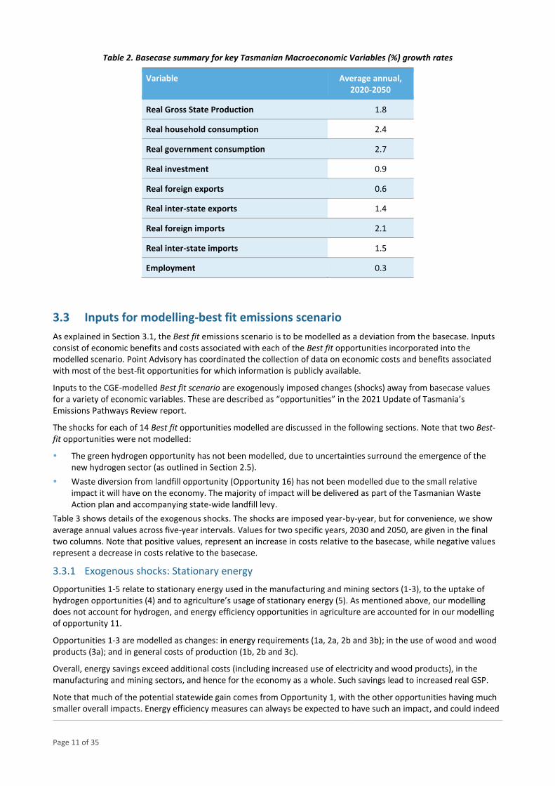
VURM traces out the implications of these inputs at a fine level of industrial and regional detail, as required for this project. Table 2 shows the average annual growth rates for key Tasmanian macroeconomic variables over 2020-2050.

– 6 Adams, P., Dixon, J. M., and Horridge, J. M. (2015). The Victoria University Regional Model (VURM): Technical Documentation, Version 1.0. Centre of Policy Studies Working Paper G-254.

Page 11 of 35

Table 2. Basecase summary for key Tasmanian Macroeconomic Variables (%) growth rates

Variable Average annual, 2020-2050

Real Gross State Production 1.8

Real household consumption 2.4

Real government consumption 2.7

Real investment 0.9

Real foreign exports 0.6

Real inter-state exports 1.4

Real foreign imports 2.1

Real inter-state imports 1.5

Employment 0.3

3.3 Inputs for modelling-best fit emissions scenario

As explained in Section 3.1, the Best fit emissions scenario is to be modelled as a deviation from the basecase. Inputs consist of economic benefits and costs associated with each of the Best fit opportunities incorporated into the modelled scenario. Point Advisory has coordinated the collection of data on economic costs and benefits associated with most of the best-fit opportunities for which information is publicly available.

Inputs to the CGE-modelled Best fit scenario are exogenously imposed changes (shocks) away from basecase values for a variety of economic variables. These are described as “opportunities” in the 2021 Update of Tasmania’s Emissions Pathways Review report.

The shocks for each of 14 Best fit opportunities modelled are discussed in the following sections. Note that two Best-fit opportunities were not modelled:

The green hydrogen opportunity has not been modelled, due to uncertainties surround the emergence of the new hydrogen sector (as outlined in Section 2.5).

Waste diversion from landfill opportunity (Opportunity 16) has not been modelled due to the small relative impact it will have on the economy. The majority of impact will be delivered as part of the Tasmanian Waste Action plan and accompanying state-wide landfill levy.

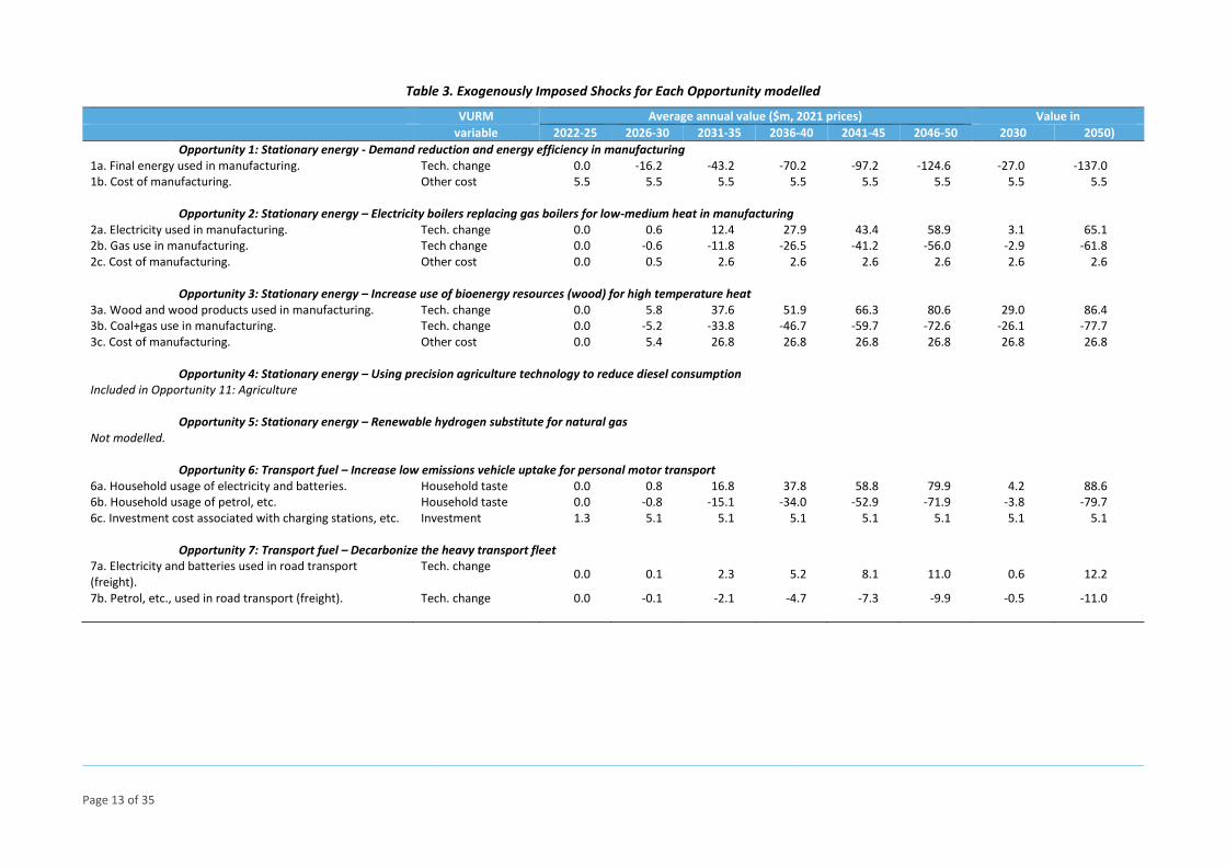
Table 3 shows details of the exogenous shocks. The shocks are imposed year-by-year, but for convenience, we show average annual values across five-year intervals. Values for two specific years, 2030 and 2050, are given in the final two columns. Note that positive values, represent an increase in costs relative to the basecase, while negative values represent a decrease in costs relative to the basecase.

3.3.1 Exogenous shocks: Stationary energy

Opportunities 1-5 relate to stationary energy used in the manufacturing and mining sectors (1-3), to the uptake of hydrogen opportunities (4) and to agriculture’s usage of stationary energy (5). As mentioned above, our modelling does not account for hydrogen, and energy efficiency opportunities in agriculture are accounted for in our modelling of opportunity 11.

Opportunities 1-3 are modelled as changes: in energy requirements (1a, 2a, 2b and 3b); in the use of wood and wood products (3a); and in general costs of production (1b, 2b and 3c).

Overall, energy savings exceed additional costs (including increased use of electricity and wood products), in the manufacturing and mining sectors, and hence for the economy as a whole. Such savings lead to increased real GSP.

Note that much of the potential statewide gain comes from Opportunity 1, with the other opportunities having much smaller overall impacts. Energy efficiency measures can always be expected to have such an impact, and could indeed

Page 12 of 35

be implemented in the basecase, but they are typically difficult to implement, due to non-financial barriers. It is assumed that the emissions reduction opportunities will require more effort than would be put into energy efficiency measures in the basecase.

3.3.2 Exogenous shocks: Transport fuel

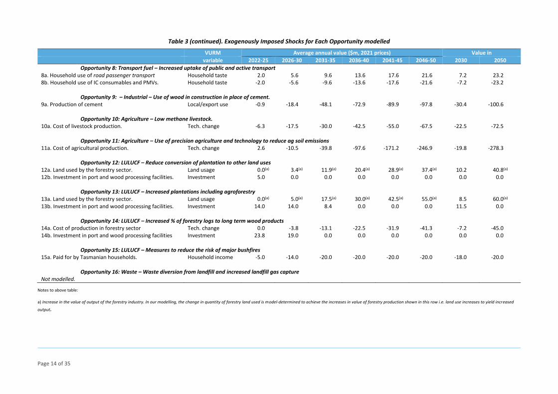
Opportunities 6-8 relate to increased replacement of internal combustion (IC) vehicles with electric and hybrid vehicles (opportunities 6 and 7), and increased uptake of public and active transportation (8).

All three opportunities are modelled as switches in demand that are nearly cost neutral. Nonetheless, because the switches are to products predominately produced in Tasmania (electricity for example) and against products produced elsewhere (petroleum for example), their overall impacts on state GSP and employment are largely positive. This remains the case even with the additional investment in charging stations, etc. (6c) accounted for.

3.3.3 Exogenous shocks: Industrial

Opportunity 9 is increased use of wood in construction in place of emissions intensive building products, notably cement. Increased wood demand is accommodated by increased wood supply arising from opportunity 14.

We assume that the rest of Australia follows suit and starts using wood in construction in place of cement. Hence local and interstate demand for Tasmanian produced cement falls.

3.3.4 Exogenous shocks: Agriculture

Opportunities 10 and 11 relate to agricultural production.

Adopting low methane production technologies (opportunity 10) delivers to the livestock industries (sheep, beef and

dairy cattle) net cost reductions. This will have a positive impact on real GSP. Similarly, the fall (relative to basecase

levels) in agricultural costs with the adoption of precision technologies (11) will benefit real GSP.

Overall, both opportunities represent a source of productivity gain for agriculture and for the economy generally.

3.3.5 Exogenous shocks: LULUCF

The final set of opportunities (12-15) relate to LULUCF activities.

The first two (12 and 13) are modelled in a similar way: increased use of land for forestry leading to increased forestry

production (12a and 13a); and increased investment in port and processing facilities to accommodate increased sales

of wood and wood/paper product (12b and 13b).

The modelling of the third opportunity in this group (14) also makes allowance for increased investment (14b), but

rather than gaining from more land, forestry gains from a reduction in unit production costs (14a).

Overall, opportunities (12-14) are likely to make a small positive contribution to real GSP, largely through the cost reductions from Opportunity 14. We assume that land converted to forestry has a largely neutral effect on real GSP because it displaces existing agricultural production earning roughly the same value added per hectare.

Opportunity 15 is different from the other LULUCF opportunities. It accounts for the increased cost of dealing with bushfires arising from expansions in forestry area. It is assumed that the immediate cost impacts fall on a mix of private and public industries, but ultimately are paid for by Tasmanian households. All else unchanged, this might be expected to lower real GSP.

3.3.6 Exogenous shocks: Waste

Opportunity 16 (Waste diversion from landfill & increase landfill gas capture) is not included in the modelling for two reasons. First, much of the impact will be delivered in the basecase, as part of the Tasmanian Waste Action plan and accompanying state-wide landfill levy. Second, even if it were not captured in the basecase, its economic impacts will be small as any costs to increase recycling and organics diversion will be fully recouped through the landfill levy.

Page 13 of 35

Table 3. Exogenously Imposed Shocks for Each Opportunity modelled

VURM Average annual value ($m, 2021 prices) Value in

variable 2022-25 2026-30 2031-35 2036-40 2041-45 2046-50 2030 2050)

Opportunity 1: Stationary energy - Demand reduction and energy efficiency in manufacturing 1a. Final energy used in manufacturing. Tech. change 0.0 -16.2 -43.2 -70.2 -97.2 -124.6 -27.0 -137.0 1b. Cost of manufacturing. Other cost 5.5 5.5 5.5 5.5 5.5 5.5 5.5 5.5

Opportunity 2: Stationary energy – Electricity boilers replacing gas boilers for low-medium heat in manufacturing 2a. Electricity used in manufacturing. Tech. change 0.0 0.6 12.4 27.9 43.4 58.9 3.1 65.1 2b. Gas use in manufacturing. Tech change 0.0 -0.6 -11.8 -26.5 -41.2 -56.0 -2.9 -61.8 2c. Cost of manufacturing. Other cost 0.0 0.5 2.6 2.6 2.6 2.6 2.6 2.6

Opportunity 3: Stationary energy – Increase use of bioenergy resources (wood) for high temperature heat 3a. Wood and wood products used in manufacturing. Tech. change 0.0 5.8 37.6 51.9 66.3 80.6 29.0 86.4 3b. Coal+gas use in manufacturing. Tech. change 0.0 -5.2 -33.8 -46.7 -59.7 -72.6 -26.1 -77.7 3c. Cost of manufacturing. Other cost 0.0 5.4 26.8 26.8 26.8 26.8 26.8 26.8

Opportunity 4: Stationary energy – Using precision agriculture technology to reduce diesel consumption Included in Opportunity 11: Agriculture

Opportunity 5: Stationary energy – Renewable hydrogen substitute for natural gas Not modelled.

Opportunity 6: Transport fuel – Increase low emissions vehicle uptake for personal motor transport 6a. Household usage of electricity and batteries. Household taste 0.0 0.8 16.8 37.8 58.8 79.9 4.2 88.6 6b. Household usage of petrol, etc. Household taste 0.0 -0.8 -15.1 -34.0 -52.9 -71.9 -3.8 -79.7 6c. Investment cost associated with charging stations, etc. Investment 1.3 5.1 5.1 5.1 5.1 5.1 5.1 5.1

Opportunity 7: Transport fuel – Decarbonize the heavy transport fleet 7a. Electricity and batteries used in road transport (freight).

Tech. change 0.0 0.1 2.3 5.2 8.1 11.0 0.6 12.2

7b. Petrol, etc., used in road transport (freight). Tech. change 0.0 -0.1 -2.1 -4.7 -7.3 -9.9 -0.5 -11.0

Page 14 of 35

Table 3 (continued). Exogenously Imposed Shocks for Each Opportunity modelled

VURM Average annual value ($m, 2021 prices) Value in

variable 2022-25 2026-30 2031-35 2036-40 2041-45 2046-50 2030 2050

Opportunity 8: Transport fuel – Increased uptake of public and active transport 8a. Household use of road passenger transport Household taste 2.0 5.6 9.6 13.6 17.6 21.6 7.2 23.2 8b. Household use of IC consumables and PMVs. Household taste -2.0 -5.6 -9.6 -13.6 -17.6 -21.6 -7.2 -23.2

Opportunity 9: – Industrial – Use of wood in construction in place of cement. 9a. Production of cement Local/export use -0.9 -18.4 -48.1 -72.9 -89.9 -97.8 -30.4 -100.6

Opportunity 10: Agriculture – Low methane livestock. 10a. Cost of livestock production. Tech. change -6.3 -17.5 -30.0 -42.5 -55.0 -67.5 -22.5 -72.5

Opportunity 11: Agriculture – Use of precision agriculture and technology to reduce ag soil emissions 11a. Cost of agricultural production. Tech. change 2.6 -10.5 -39.8 -97.6 -171.2 -246.9 -19.8 -278.3

Opportunity 12: LULUCF – Reduce conversion of plantation to other land uses 12a. Land used by the forestry sector. Land usage 0.0(a) 3.4(a) 11.9(a) 20.4(a) 28.9(a) 37.4(a) 10.2 40.8(a) 12b. Investment in port and wood processing facilities. Investment 5.0 0.0 0.0 0.0 0.0 0.0 0.0 0.0

Opportunity 13: LULUCF – Increased plantations including agroforestry 13a. Land used by the forestry sector. Land usage 0.0(a) 5.0(a) 17.5(a) 30.0(a) 42.5(a) 55.0(a) 8.5 60.0(a) 13b. Investment in port and wood processing facilities. Investment 14.0 14.0 8.4 0.0 0.0 0.0 11.5 0.0

Opportunity 14: LULUCF – Increased % of forestry logs to long term wood products 14a. Cost of production in forestry sector Tech. change 0.0 -3.8 -13.1 -22.5 -31.9 -41.3 -7.2 -45.0 14b. Investment in port and wood processing facilities Investment 23.8 19.0 0.0 0.0 0.0 0.0 0.0 0.0

Opportunity 15: LULUCF – Measures to reduce the risk of major bushfires 15a. Paid for by Tasmanian households. Household income -5.0 -14.0 -20.0 -20.0 -20.0 -20.0 -18.0 -20.0

Opportunity 16: Waste – Waste diversion from landfill and increased landfill gas capture Not modelled.

Notes to above table:

a) Increase in the value of output of the forestry industry. In our modelling, the change in quantity of forestry land used is model-determined to achieve the increases in value of forestry production shown in this row i.e. land use increases to yield increased

output.

Page 15 of 35

3.4 Simulation design

The alternative (Best fit) simulation deviates away from the basecase in response to the shocks described in Section 3.3. Underlying these deviations are a number of assumptions relating to the behaviour of key macroeconomic variables. The key assumptions are explained in the following sections.

3.4.1 Labour markets

Labour is assumed mobile between state economies. Labour is assumed to move between regions to maintain inter-state unemployment-rate differentials at their basecase-case levels. Accordingly, Tasmania, which is relatively favourably affected by changes away from basecase due to emissions reduction opportunities uptake, is allowed to experience increases in its labour forces as well as in employment, at the expense of the Rest of Australia (RoA).

3.4.2 Private consumption and investment

Private consumption expenditure is determined via a consumption function that links nominal consumption to household disposable income (HDI). Investment in all but a few industries is allowed to deviate from its basecase value in line with deviations in expected rates of return on the industries’ capital stocks.

In the Best fit emissions scenario, VURM allows for short-run divergences in rates of return from their basecase levels. These cause divergences in investment and hence capital stocks that gradually erode the initial divergences in rates of return.

3.4.3 Government consumption and fiscal balances

VURM contains no theory to explain changes in real public consumption. For these simulations, public consumption (Federal and state) is simply held fixed. The fiscal balances of each jurisdiction (federal, state and territory) as a share of nominal GDP are allowed to vary relative to reference case values in line with projected changes in government expenditure and income.

3.4.4 Production technologies and household tastes

VURM contains many variables to allow for shifts in technology and household preferences. In the Best fit scenario, most of these variables are exogenous and have the same values as in the basecase projection. The exceptions are technology and taste (preferences) variables, used to introduce shocks to the model (see Table 3).

Page 16 of 35

4 RESULTS AND ANALYSIS

The following sections provide the results of the CGE modelling showing the impact of the roll-out of the best-fit emissions opportunities on Tasmania’s Real GSP, overall and industry specific employment, and industry output.

4.1 Economic impacts

Results are presented as deviations from the basecase in which none of the opportunities captured in Best fit are taken up. This is the conventional approach with comparative dynamics in VURM and most other CGE models.

Below we explain results for real GSP, total employment and real value added by ANZSIC division. More detailed results for ANZSIC division and the 83 industries recognized in VURM are given in the Appendix:

Table 4: Absolute changes ($m, 2021 prices) from basecase in real value added by ANZSIC division;

Table 5: Percentage changes from basecase in real value added by ANZSIC division;

Table 6: Absolute changes (’00 full and part-time jobs) from basecase in employment by ANZSIC division;

Table 7: Percentage changes from basecase in employment by ANZSIC division;

Table 8 to Table 11– corresponding results by VURM industry.

Note that the ANZSIC division results are aggregations of the VURM industry results.

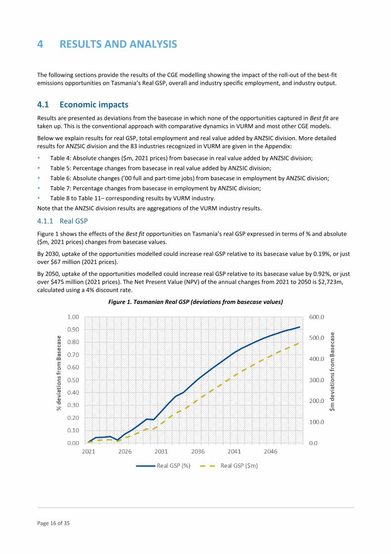
4.1.1 Real GSP

Figure 1 shows the effects of the Best fit opportunities on Tasmania’s real GSP expressed in terms of % and absolute ($m, 2021 prices) changes from basecase values.

By 2030, uptake of the opportunities modelled could increase real GSP relative to its basecase value by 0.19%, or just over $67 million (2021 prices).

By 2050, uptake of the opportunities modelled could increase real GSP relative to its basecase value by 0.92%, or just over $475 million (2021 prices). The Net Present Value (NPV) of the annual changes from 2021 to 2050 is $2,723m, calculated using a 4% discount rate.

Figure 1. Tasmanian Real GSP (deviations from basecase values)

Page 17 of 35

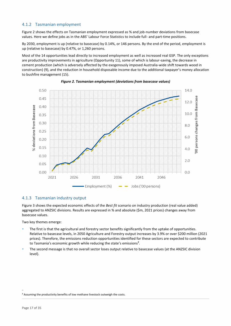
4.1.2 Tasmanian employment

Figure 2 shows the effects on Tasmanian employment expressed as % and job-number deviations from basecase values. Here we define jobs as in the ABS’ Labour Force Statistics to include full- and part-time positions.

By 2030, employment is up (relative to basecase) by 0.14%, or 146 persons. By the end of the period, employment is up (relative to basecase) by 0.47%, or 1,260 persons.

Most of the 14 opportunities lead directly to increased employment as well as increased real GSP. The only exceptions are productivity improvements in agriculture (Opportunity 11), some of which is labour-saving, the decrease in cement production (which is adversely affected by the exogenously imposed Australia-wide shift towards wood in construction) (9), and the reduction in household disposable income due to the additional taxpayer’s money allocation to bushfire management (15).

Figure 2. Tasmanian employment (deviations from basecase values)

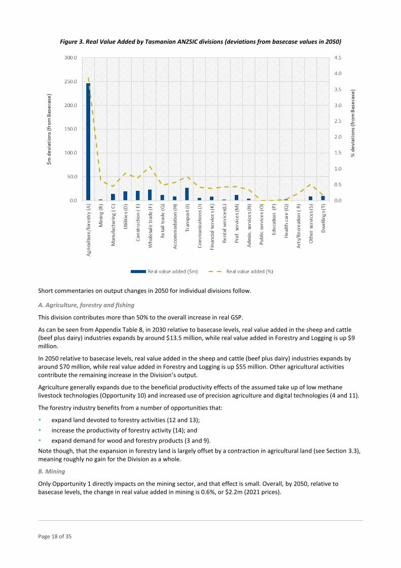
4.1.3 Tasmanian industry output

Figure 3 shows the expected economic effects of the Best fit scenario on industry production (real value added) aggregated to ANZSIC divisions. Results are expressed in % and absolute ($m, 2021 prices) changes away from basecase values.

Two key themes emerge:

The first is that the agricultural and forestry sector benefits significantly from the uptake of opportunities. Relative to basecase levels, in 2050 Agriculture and Forestry output increases by 3.9% or over $200 million (2021 prices). Therefore, the emissions reduction opportunities identified for these sectors are expected to contribute to Tasmania’s economic growth while reducing the state’s emissions7.

The second message is that no overall sector loses output relative to basecase values (at the ANZSIC division level).

–

7 Assuming the productivity benefits of low methane livestock outweigh the costs.

Page 18 of 35

Figure 3. Real Value Added by Tasmanian ANZSIC divisions (deviations from basecase values in 2050)

Short commentaries on output changes in 2050 for individual divisions follow.

A. Agriculture, forestry and fishing

This division contributes more than 50% to the overall increase in real GSP.

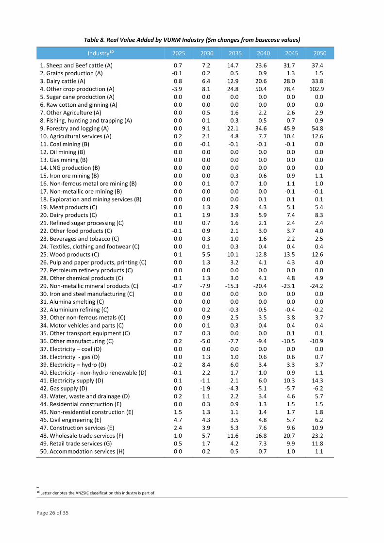
As can be seen from Appendix Table 8, in 2030 relative to basecase levels, real value added in the sheep and cattle (beef plus dairy) industries expands by around $13.5 million, while real value added in Forestry and Logging is up $9 million.

In 2050 relative to basecase levels, real value added in the sheep and cattle (beef plus dairy) industries expands by around $70 million, while real value added in Forestry and Logging is up $55 million. Other agricultural activities contribute the remaining increase in the Division’s output.

Agriculture generally expands due to the beneficial productivity effects of the assumed take up of low methane livestock technologies (Opportunity 10) and increased use of precision agriculture and digital technologies (4 and 11).

The forestry industry benefits from a number of opportunities that:

expand land devoted to forestry activities (12 and 13);

increase the productivity of forestry activity (14); and

expand demand for wood and forestry products (3 and 9).

Note though, that the expansion in forestry land is largely offset by a contraction in agricultural land (see Section 3.3), meaning roughly no gain for the Division as a whole.

B. Mining

Only Opportunity 1 directly impacts on the mining sector, and that effect is small. Overall, by 2050, relative to basecase levels, the change in real value added in mining is 0.6%, or $2.2m (2021 prices).

Page 19 of 35

C. Manufacturing

Relative to its basecase level, real value added in Manufacturing expands by 0.1%, or $1.8m (2021 prices) by 2030, and by 0.4%, or $13.5m (2021 prices) by 2050. This is the net outcome of a number of positive and negative effects.

Manufacturing industries that gain most (see Table 8) are as follows.

Industries producing food and drink products (industries 19-23). These are favoured by being trade-exposed and, hence, facing relatively flat demand curves. Productivity improvements in agriculture lead to reduced costs for food and drink producers and subsequently increased production, particularly for interstate and overseas exports.

Industries producing wood and paper products (25 and 26). These are favoured directly and indirectly (via increased plantation forestry activity) by the uptake of opportunities 3a and 12-14.

Other chemical products (industry 28). The main customer for this industry is the expanded agricultural sector through purchases of farm chemicals and fertiliser.

The following manufacturing industries experience a lower level of GSP (relative to basecase levels).

Non-metallic mineral products (industry 29). Its main product is cement (and concrete) which is adversely affected by the exogenously imposed Australia-wide shift towards wood in construction (Opportunity 9)

Aluminium (32). The very small contraction is due to a slight rise in the price of its major input – electricity. Electricity’s price is up due to increased demand arising particularly from the uptake of opportunities 2, 6 and 7.

Other manufacturing (36). This industry produces a range of products sold primarily to households. The industry is hit by a reduction in Household use of passenger motor vehicles and internal-combustion consumables such as conventional batteries following the uptake of Opportunities 6 and 8.

D. Electricity, gas and water/waste services

Relative to its basecase level, real value added in this division is up 0.7%, or $10m (2021 prices) by 2030, and is up 0.9%, or $19.4m (2021 prices) by 2050. The increase in output is in line with the increase in real GSP which is to be expected given the wide-spread nature of this Division’s sales. However, the increase is not uniform within the sector. As can be seen from Table 9, production of electricity rises by more than real GSP in percentage terms, while production of gas services falls. These contrasting changes reflect the uptake of various energy-related technological changes under opportunities 1-3 and 6-7. In overall terms, these favour the use of electricity and oppose the use of gas (and imported petroleum products).

E. Construction

Production of construction services rises (compared to basecase) by 0.4%, or $8m (2021 prices) by 2030, and by 0.7%, or $20.5m (2021 prices) by 2050. This is in line with the general expansion in the economy and the slight increase in capital that supports the larger economy.

Note that in earlier years, construction spending is boosted by opportunity-specific investments in port and wood processing facilities under Opportunities 12, 13 and 14. However, this additional investment has finished well before 2050.

F. Wholesale trade

In percentage terms, output in this division rises a little more than real GSP (1.1% cf. 0.9%) by 2050. This is due to its sales structure being slightly more-oriented towards commercial customers in agriculture and food processing. These industries achieve outputs gains which, in percentage terms, is higher than the economy-wide average.

G. Retail trade – T. Ownership of dwellings

The remaining divisions are focussed on domestic final consumption (household and government) and on interstate and international tourism.

Government consumption, by assumption, is held fixed at basecase values (Section 3.4).

Visitation from overseas or interstate is not directly affected by uptake of any of the opportunities.

Household consumption rises relative to its basecase level, but by less than real GDP (reflecting, in a small part, the effects of Opportunity 15).

Thus, generally, the impacts on these remaining divisions are relatively small. This is especially the case for the government focussed Division O - Public administration and safety, and Division P - Education and training.

Page 20 of 35

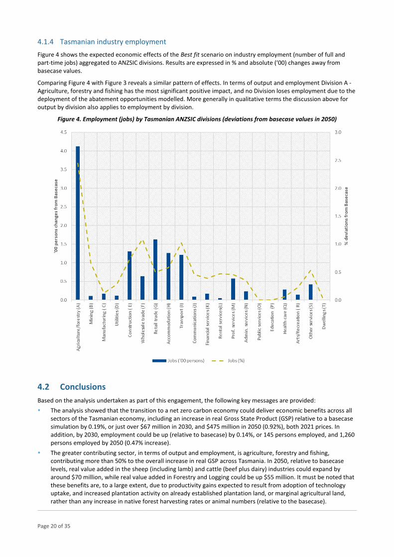
4.1.4 Tasmanian industry employment

Figure 4 shows the expected economic effects of the Best fit scenario on industry employment (number of full and part-time jobs) aggregated to ANZSIC divisions. Results are expressed in % and absolute (‘00) changes away from basecase values.

Comparing Figure 4 with Figure 3 reveals a similar pattern of effects. In terms of output and employment Division A - Agriculture, forestry and fishing has the most significant positive impact, and no Division loses employment due to the deployment of the abatement opportunities modelled. More generally in qualitative terms the discussion above for output by division also applies to employment by division.

Figure 4. Employment (jobs) by Tasmanian ANZSIC divisions (deviations from basecase values in 2050)

4.2 Conclusions

Based on the analysis undertaken as part of this engagement, the following key messages are provided:

The analysis showed that the transition to a net zero carbon economy could deliver economic benefits across all sectors of the Tasmanian economy, including an increase in real Gross State Product (GSP) relative to a basecase simulation by 0.19%, or just over $67 million in 2030, and $475 million in 2050 (0.92%), both 2021 prices. In addition, by 2030, employment could be up (relative to basecase) by 0.14%, or 145 persons employed, and 1,260 persons employed by 2050 (0.47% increase).

The greater contributing sector, in terms of output and employment, is agriculture, forestry and fishing, contributing more than 50% to the overall increase in real GSP across Tasmania. In 2050, relative to basecase levels, real value added in the sheep (including lamb) and cattle (beef plus dairy) industries could expand by around $70 million, while real value added in Forestry and Logging could be up $55 million. It must be noted that these benefits are, to a large extent, due to productivity gains expected to result from adoption of technology uptake, and increased plantation activity on already established plantation land, or marginal agricultural land, rather than any increase in native forest harvesting rates or animal numbers (relative to the basecase).

Page 21 of 35

Other important sectors include manufacturing, which expands, relative to its basecase level, by 0.1%, or $1.8m (2021 prices) by 2030, and by 0.4%, or $13.5m (2021 prices) by 2050. Production of construction services rises (compared to basecase) by 0.4%, or $8m (2021 prices) by 2030, and by 0.7%, or $20.5m (2021 prices) by 2050, while collectively ANZSIC Divisions F to T (see Appendix 3) expand by $26.5m (2021 prices) by 2030, and by $123.5m by 2050.

Importantly, under the assumptions made, no ANZSC division would lose significant employment due to the deployment of the best-fit emissions reduction opportunities modelled, although there may be some reallocation within sectors in favor of less emission intensive production processes.

Page 22 of 35

APPENDIX 1 ADDITIONAL VURM INFORMATION

Each region in VURM has a single representative household, and a single state/local government agent. The federal government operates in each region. The foreign sector is described by export demand curves for the products of each region, and by supply curves for international imports to each region. Supply and demand for each regionally-produced commodity is the outcome of optimising behavior. Regional industries are assumed to use intermediate inputs, labour, capital and land in a cost-minimising way, while operating in competitive markets. Region-specific representative households purchase utility-maximising bundles of goods, subject to given prices and disposable income. Regions are linked via interregional trade, interregional migration and capital movements, and governments operate within a fiscal federal framework.

Investment in each regional industry is positively related to expected rates of return on capital in each regional industry. VURM recognizes two investor classes: local investors (i.e. domestic households and government) and foreign investors. Capital creators assemble, in a cost-minimizing manner, units of industry-specific physical capital for each regional industry.

VURM normally provides results for economic variables on a year-on-year basis. The results for a particular year are used to update the database for the commencement of the next year. More specifically, the model contains a series of equations that connect capital stocks to past-year capital stocks and net investment. Similarly, debt is linked to past and present borrowing/saving, and the regional population is related to natural growth and international and interstate migration. The model is solved with the GEMPACK software package (Horrdige et.al., 20188).

VURM is parameterized using data from a variety of sources, including Australian Bureau of Statistics (ABS) census statistics and data from the ABS’ state accounts, international trade, labour force and demographic publications. The core VURM model database underwent a significant update during the first half of 2020 to incorporate the ABS 2016/17 Input-Output data release, together with updated Government Financial Statistics information.

This calibration procedure produces a core database for the financial year 2016/17. This is updated via model simulation to the reference year for the simulations reported year of 2019/20 (hereinafter 2020). The historical updating utilises published statistics for the period 2016/17 to 2019/20, along with extrapolated information for unobserved variables that determine, for example, changes in industry technologies and household tastes.

APPENDIX 2 EQUATIONS USED TO UNDERSTAND VURM GSP CALCULATIONS

To understand the impacts of the best-fit opportunities on real GSP discussed in Section 4.1.1, we use the following Back-Of-The-Envelope (BOTE) equation. It explains the percentage change in real GSP from the supply (or input) side as the sum of contribution made by percentage changes in factor inputs (labour, capital and land) plus the cost saving associated with productivity improvements.9

In mathematical terms,

% % % % /L K LandGDP S L S K S Land PROD GDP = + + + (1)

On the left hand side of equation (1) is the percentage change in real GSP. On the right hand side, we start with the product of the share of labour and the percentage change in employment. Subsequently we have the share of capital times the percentage change in capital, the share of land time the percentage change in land, and finally productivity improving cost reductions (PROD) as a share of GDP (GDP). The first three products are the contributions from changes in each factor input. The final term is the contribution from productivity improvement.

– 8 Horridge, J. M., Jerie, M., Mustakinov, D., and Schiffmann, F. (2018). GEMPACK manual, GEMPACK Software. Centre of Policy Studies, Victoria University, Melbourne, ISBN 978-1-921654-34-3.

9 Recall, that real GDP from the supply side equals the real cost of factor inputs + the value of productivity improvements plus the real collection of indirect taxes net of subsidies. In what follows, we ignore indirect taxes because they are small to begin with and uptake of the abatement opportunities has relatively little effect on their collection.

Page 23 of 35

According to our basecase, in 2050, SL = 0.5, SK = 0.4 and SLand = 0.1. Together, in 2050 the net cost reductions from opportunities 1, 2, 3, 10, 11 and 14a yield an increase in productivity of $427m, or 0.8% of real GDP. The overall quantity of land in Tasmania does not change as a result of implementing the opportunities – more land is used for forestry, but this is offset by less land used for agriculture. Hence, %ΔLand = 0.

Putting these values into (1) gives:

% 0.5 % 0.4 % 0 0.8GDP L K = + + + (2).

In terms of Full Time Equivalent (FTE) units, in 2050 Tasmania’s employment is projected to rise by 0.3% relative to its basecase level. Capital follows with a similar increase of 0.3%. Increased factor inputs emanate, in the main, from the exogenously imposed demand-side changes. Overall, these favour Tasmanian-produced products even with the cut in cement production (Opportunity 9) and the fall in household income available for consumption (15) accounted for.

Inserting these values into equation (2) yields a BOTE-estimate for the percentage change in real GDP of 1.1 ( = 0.3 + 0.8)%. This compares to the final VURM-projection of 0.9%. The difference of 0.2 percentage points can be attributable to factors not accounted for in our BOTE equation, including income-induced shifts in the economic structure of the economy that can add to, or detract from, the overall change in real GSP.

Though our BOTE explanation is not perfect, it does serve two important purposes. First, it gives us confidence that VURM’s projection of real GSP gain in response to the exogenous changes given in Table 3 is of the right order of magnitude. Second, it shows how important are the productivity improvements in delivering the final positive GSP result.

APPENDIX 3 DETAILED INDUSTRY RESULTS

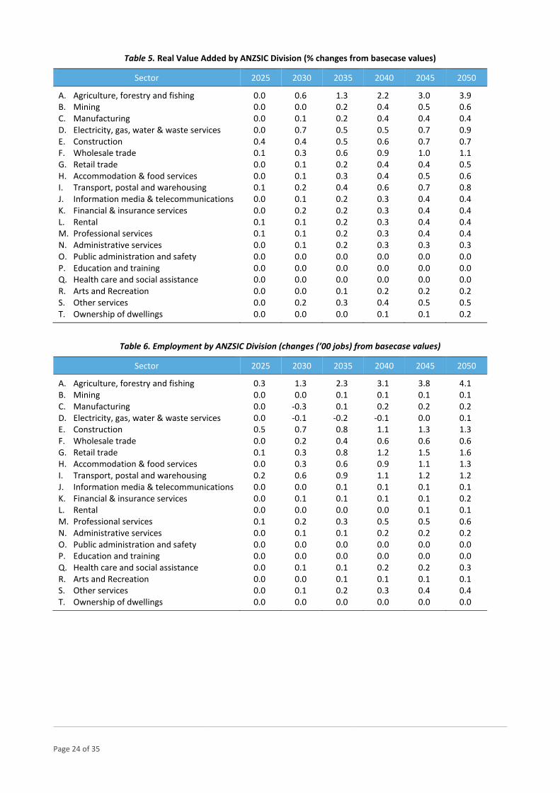
Table 4. Real Value Added by ANZSIC Division ($m changes from basecase values)

Sector 2025 2030 2035 2040 2045 2050

A. Agriculture, forestry and fishing -2.4 33.7 81.6 140.6 199.0 246.8 B. Mining -0.1 0.0 0.8 1.5 1.9 2.2 C. Manufacturing 0.3 1.8 7.7 11.9 13.8 13.5 D. Electricity, gas, water & waste services 0.0 10.0 8.7 9.3 14.1 19.4 E. Construction 8.6 9.9 10.8 15.1 18.4 20.5 F. Wholesale trade 1.0 5.7 11.6 16.8 20.7 23.2 G. Retail trade 0.5 1.7 4.2 7.3 9.9 11.8 H. Accommodation & food services 0.0 1.3 3.3 5.2 7.0 8.5 I. Transport, postal and warehousing 1.8 7.8 14.4 20.1 24.3 26.6 J. Information media & telecommunications 0.1 1.0 2.5 3.6 4.6 5.5 K. Financial & insurance services 0.2 2.0 3.2 4.8 6.6 8.2 L. Rental 0.2 0.5 0.8 1.2 1.6 2.0 M. Professional services 1.1 2.9 5.3 7.9 10.2 12.0 N. Administrative services 0.2 0.8 1.5 2.3 3.1 3.7 O. Public administration and safety 0.0 0.0 0.0 0.0 0.0 0.0 P. Education and training 0.0 0.0 0.0 0.0 0.0 0.0 Q. Health care and social assistance 0.0 0.6 1.0 1.5 2.1 2.6 R. Arts and Recreation 0.0 0.1 0.3 0.5 0.8 0.9 S. Other services 0.4 1.9 3.8 5.8 7.6 9.1 T. Ownership of dwellings 0.1 0.3 1.7 4.0 6.7 9.3

Page 24 of 35

Table 5. Real Value Added by ANZSIC Division (% changes from basecase values)

Sector 2025 2030 2035 2040 2045 2050

A. Agriculture, forestry and fishing 0.0 0.6 1.3 2.2 3.0 3.9 B. Mining 0.0 0.0 0.2 0.4 0.5 0.6 C. Manufacturing 0.0 0.1 0.2 0.4 0.4 0.4 D. Electricity, gas, water & waste services 0.0 0.7 0.5 0.5 0.7 0.9 E. Construction 0.4 0.4 0.5 0.6 0.7 0.7 F. Wholesale trade 0.1 0.3 0.6 0.9 1.0 1.1 G. Retail trade 0.0 0.1 0.2 0.4 0.4 0.5 H. Accommodation & food services 0.0 0.1 0.3 0.4 0.5 0.6 I. Transport, postal and warehousing 0.1 0.2 0.4 0.6 0.7 0.8 J. Information media & telecommunications 0.0 0.1 0.2 0.3 0.4 0.4 K. Financial & insurance services 0.0 0.2 0.2 0.3 0.4 0.4 L. Rental 0.1 0.1 0.2 0.3 0.4 0.4 M. Professional services 0.1 0.1 0.2 0.3 0.4 0.4 N. Administrative services 0.0 0.1 0.2 0.3 0.3 0.3 O. Public administration and safety 0.0 0.0 0.0 0.0 0.0 0.0 P. Education and training 0.0 0.0 0.0 0.0 0.0 0.0 Q. Health care and social assistance 0.0 0.0 0.0 0.0 0.0 0.0 R. Arts and Recreation 0.0 0.0 0.1 0.2 0.2 0.2 S. Other services 0.0 0.2 0.3 0.4 0.5 0.5 T. Ownership of dwellings 0.0 0.0 0.0 0.1 0.1 0.2

Table 6. Employment by ANZSIC Division (changes (’00 jobs) from basecase values)

Sector 2025 2030 2035 2040 2045 2050

A. Agriculture, forestry and fishing 0.3 1.3 2.3 3.1 3.8 4.1 B. Mining 0.0 0.0 0.1 0.1 0.1 0.1 C. Manufacturing 0.0 -0.3 0.1 0.2 0.2 0.2 D. Electricity, gas, water & waste services 0.0 -0.1 -0.2 -0.1 0.0 0.1 E. Construction 0.5 0.7 0.8 1.1 1.3 1.3 F. Wholesale trade 0.0 0.2 0.4 0.6 0.6 0.6 G. Retail trade 0.1 0.3 0.8 1.2 1.5 1.6 H. Accommodation & food services 0.0 0.3 0.6 0.9 1.1 1.3 I. Transport, postal and warehousing 0.2 0.6 0.9 1.1 1.2 1.2 J. Information media & telecommunications 0.0 0.0 0.1 0.1 0.1 0.1 K. Financial & insurance services 0.0 0.1 0.1 0.1 0.1 0.2 L. Rental 0.0 0.0 0.0 0.0 0.1 0.1 M. Professional services 0.1 0.2 0.3 0.5 0.5 0.6 N. Administrative services 0.0 0.1 0.1 0.2 0.2 0.2 O. Public administration and safety 0.0 0.0 0.0 0.0 0.0 0.0 P. Education and training 0.0 0.0 0.0 0.0 0.0 0.0 Q. Health care and social assistance 0.0 0.1 0.1 0.2 0.2 0.3 R. Arts and Recreation 0.0 0.0 0.1 0.1 0.1 0.1 S. Other services 0.0 0.1 0.2 0.3 0.4 0.4 T. Ownership of dwellings 0.0 0.0 0.0 0.0 0.0 0.0

Page 25 of 35

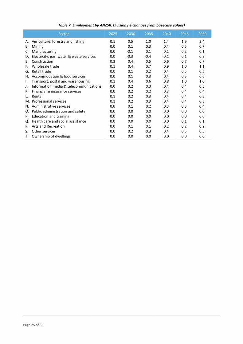
Table 7. Employment by ANZSIC Division (% changes from basecase values)

Sector 2025 2030 2035 2040 2045 2050

A. Agriculture, forestry and fishing 0.1 0.5 1.0 1.4 1.9 2.4 B. Mining 0.0 0.1 0.3 0.4 0.5 0.7 C. Manufacturing 0.0 -0.1 0.1 0.1 0.2 0.1 D. Electricity, gas, water & waste services 0.0 -0.3 -0.4 -0.1 0.1 0.3 E. Construction 0.3 0.4 0.5 0.6 0.7 0.7 F. Wholesale trade 0.1 0.4 0.7 0.9 1.0 1.1 G. Retail trade 0.0 0.1 0.2 0.4 0.5 0.5 H. Accommodation & food services 0.0 0.1 0.3 0.4 0.5 0.6 I. Transport, postal and warehousing 0.1 0.4 0.6 0.8 1.0 1.0 J. Information media & telecommunications 0.0 0.2 0.3 0.4 0.4 0.5 K. Financial & insurance services 0.0 0.2 0.2 0.3 0.4 0.4 L. Rental 0.1 0.2 0.3 0.4 0.4 0.5 M. Professional services 0.1 0.2 0.3 0.4 0.4 0.5 N. Administrative services 0.0 0.1 0.2 0.3 0.3 0.4 O. Public administration and safety 0.0 0.0 0.0 0.0 0.0 0.0 P. Education and training 0.0 0.0 0.0 0.0 0.0 0.0 Q. Health care and social assistance 0.0 0.0 0.0 0.0 0.1 0.1 R. Arts and Recreation 0.0 0.1 0.1 0.2 0.2 0.2 S. Other services 0.0 0.2 0.3 0.4 0.5 0.5 T. Ownership of dwellings 0.0 0.0 0.0 0.0 0.0 0.0

Page 26 of 35

Table 8. Real Value Added by VURM Industry ($m changes from basecase values)

Industry10 2025 2030 2035 2040 2045 2050

1. Sheep and Beef cattle (A) 0.7 7.2 14.7 23.6 31.7 37.4 2. Grains production (A) -0.1 0.2 0.5 0.9 1.3 1.5 3. Dairy cattle (A) 0.8 6.4 12.9 20.6 28.0 33.8 4. Other crop production (A) -3.9 8.1 24.8 50.4 78.4 102.9 5. Sugar cane production (A) 0.0 0.0 0.0 0.0 0.0 0.0 6. Raw cotton and ginning (A) 0.0 0.0 0.0 0.0 0.0 0.0 7. Other Agriculture (A) 0.0 0.5 1.6 2.2 2.6 2.9 8. Fishing, hunting and trapping (A) 0.0 0.1 0.3 0.5 0.7 0.9 9. Forestry and logging (A) 0.0 9.1 22.1 34.6 45.9 54.8 10. Agricultural services (A) 0.2 2.1 4.8 7.7 10.4 12.6 11. Coal mining (B) 0.0 -0.1 -0.1 -0.1 -0.1 0.0 12. Oil mining (B) 0.0 0.0 0.0 0.0 0.0 0.0 13. Gas mining (B) 0.0 0.0 0.0 0.0 0.0 0.0 14. LNG production (B) 0.0 0.0 0.0 0.0 0.0 0.0 15. Iron ore mining (B) 0.0 0.0 0.3 0.6 0.9 1.1 16. Non-ferrous metal ore mining (B) 0.0 0.1 0.7 1.0 1.1 1.0 17. Non-metallic ore mining (B) 0.0 0.0 0.0 0.0 -0.1 -0.1 18. Exploration and mining services (B) 0.0 0.0 0.0 0.1 0.1 0.1 19. Meat products (C) 0.0 1.3 2.9 4.3 5.1 5.4 20. Dairy products (C) 0.1 1.9 3.9 5.9 7.4 8.3 21. Refined sugar processing (C) 0.0 0.7 1.6 2.1 2.4 2.4 22. Other food products (C) -0.1 0.9 2.1 3.0 3.7 4.0 23. Beverages and tobacco (C) 0.0 0.3 1.0 1.6 2.2 2.5 24. Textiles, clothing and footwear (C) 0.0 0.1 0.3 0.4 0.4 0.4 25. Wood products (C) 0.1 5.5 10.1 12.8 13.5 12.6 26. Pulp and paper products, printing (C) 0.0 1.3 3.2 4.1 4.3 4.0 27. Petroleum refinery products (C) 0.0 0.0 0.0 0.0 0.0 0.0 28. Other chemical products (C) 0.1 1.3 3.0 4.1 4.8 4.9 29. Non-metallic mineral products (C) -0.7 -7.9 -15.3 -20.4 -23.1 -24.2 30. Iron and steel manufacturing (C) 0.0 0.0 0.0 0.0 0.0 0.0 31. Alumina smelting (C) 0.0 0.0 0.0 0.0 0.0 0.0 32. Aluminium refining (C) 0.0 0.2 -0.3 -0.5 -0.4 -0.2 33. Other non-ferrous metals (C) 0.0 0.9 2.5 3.5 3.8 3.7 34. Motor vehicles and parts (C) 0.0 0.1 0.3 0.4 0.4 0.4 35. Other transport equipment (C) 0.7 0.3 0.0 0.0 0.1 0.1 36. Other manufacturing (C) 0.2 -5.0 -7.7 -9.4 -10.5 -10.9 37. Electricity – coal (D) 0.0 0.0 0.0 0.0 0.0 0.0 38. Electricity - gas (D) 0.0 1.3 1.0 0.6 0.6 0.7 39. Electricity – hydro (D) -0.2 8.4 6.0 3.4 3.3 3.7 40. Electricity - non-hydro renewable (D) -0.1 2.2 1.7 1.0 0.9 1.1 41. Electricity supply (D) 0.1 -1.1 2.1 6.0 10.3 14.3 42. Gas supply (D) 0.0 -1.9 -4.3 -5.1 -5.7 -6.2 43. Water, waste and drainage (D) 0.2 1.1 2.2 3.4 4.6 5.7 44. Residential construction (E) 0.0 0.3 0.9 1.3 1.5 1.5 45. Non-residential construction (E) 1.5 1.3 1.1 1.4 1.7 1.8 46. Civil engineering (E) 4.7 4.3 3.5 4.8 5.7 6.2 47. Construction services (E) 2.4 3.9 5.3 7.6 9.6 10.9 48. Wholesale trade services (F) 1.0 5.7 11.6 16.8 20.7 23.2 49. Retail trade services (G) 0.5 1.7 4.2 7.3 9.9 11.8 50. Accommodation services (H) 0.0 0.2 0.5 0.7 1.0 1.1

– 10 Letter denotes the ANZSIC classification this industry is part of.

Page 27 of 35

Table 8 (continued). Real Value Added by VURM Industry ($m changes from basecase values)

Industry 2025 2030 2035 2040 2045 2050

51. Restaurant and food services (H) 0.0 1.1 2.8 4.5 6.1 7.4 52. Road freight transport (I) 0.3 3.6 7.3 10.0 11.4 11.8 53. Road passenger transport (I) 1.5 3.4 5.2 6.7 8.1 9.1 54. Rail freight transport (I) 0.0 0.0 0.1 0.2 0.3 0.3 55. Rail passenger transport (I) 0.0 0.0 0.0 0.1 0.1 0.1 56. Air transport services (I) 0.0 0.3 1.0 1.6 2.1 2.6 57. Water and other transport services (I) 0.0 0.4 0.8 1.6 2.3 2.7 58. Communication services (J) 0.1 1.0 2.5 3.6 4.6 5.5 59. Banking services (K) 0.1 1.1 1.9 2.8 3.8 4.8 60. Insurance services (K) 0.1 0.7 1.1 1.6 2.2 2.7 61. Superannuation services (K) 0.0 0.1 0.2 0.4 0.6 0.8 62. Non-real estate rental and hiring (L) 0.2 0.5 0.8 1.2 1.6 2.0 63. Ownership of Dwellings (T) 0.1 0.3 1.7 4.0 6.7 9.3 64. Real estate business services (M) 0.3 1.1 2.2 3.3 4.2 4.8 65. Legal services (M) 0.1 0.2 0.3 0.4 0.5 0.6 66. Professional/Scientific/Technical (M) 0.7 1.6 2.8 4.3 5.6 6.5 67. Other business services (N) 0.2 0.8 1.5 2.3 3.1 3.7 68. Public administration (O) 0.0 0.0 0.0 0.0 0.0 0.0 69. Defence services (O) 0.0 0.0 0.0 0.0 0.0 0.0 70. Pre-school education services (P) 0.0 0.0 0.0 0.0 0.0 0.0 71. Primary school education services (P) 0.0 0.0 0.0 0.0 0.0 0.0 72. Secondary school education services (P) 0.0 0.0 0.0 0.0 0.0 0.0 73. Technical education services (P) 0.0 0.0 0.0 0.0 0.0 0.0 74. Tertiary education services (P) 0.0 0.0 0.0 0.0 0.0 0.0 75. Health care services (Q) 0.0 0.3 0.5 0.8 1.1 1.4 76. Residential care services (Q) 0.0 0.1 0.1 0.1 0.2 0.3 77. Child care services (Q) 0.0 0.1 0.2 0.3 0.4 0.5 78. Other care services (Q) 0.0 0.1 0.2 0.3 0.4 0.4 79. Arts and recreational services (R) 0.0 0.1 0.2 0.3 0.4 0.5 80. Gambling services (R) 0.0 0.0 0.1 0.2 0.3 0.4 81. Other services (S) 0.4 1.9 3.8 5.8 7.6 9.1

Page 28 of 35

Table 9. Real Value Added by VURM Industry (% changes from basecase values)

Industry 2025 2030 2035 2040 2045 2050

1. Sheep and Beef cattle (A) 0.1 1.2 2.3 3.6 4.9 6.1 2. Grains production (A) -0.2 0.6 1.6 2.9 4.3 5.5 3. Dairy cattle (A) 0.2 1.3 2.4 3.8 5.3 6.8 4. Other crop production (A) -0.2 0.3 0.9 1.7 2.7 3.6 5. Sugar cane production (A) 0.0 0.0 0.0 0.0 0.0 0.0 6. Raw cotton and ginning (A) 0.0 0.0 0.0 0.0 0.0 0.0 7. Other Agriculture (A) 0.0 0.1 0.2 0.2 0.3 0.3 8. Fishing, hunting and trapping (A) 0.0 0.0 0.1 0.2 0.3 0.3 9. Forestry and logging (A) 0.0 1.4 3.0 4.5 5.7 6.9 10. Agricultural services (A) 0.0 0.6 1.3 1.9 2.5 3.0 11. Coal mining (B) -0.1 -4.8 -7.6 -8.7 -7.6 -5.5 12. Oil mining (B) 0.0 0.0 0.0 0.0 0.0 0.0 13. Gas mining (B) 0.0 0.0 0.0 0.0 0.0 0.0 14. LNG production (B) 0.0 0.0 0.0 0.0 0.0 0.0 15. Iron ore mining (B) 0.0 0.0 0.1 0.3 0.4 0.5 16. Nonferrous metal ore mining (B) 0.0 0.1 0.5 0.8 1.1 1.3 17. Non-metallic ore mining (B) 0.0 -0.2 -0.4 -0.7 -1.0 -1.3 18. Exploration and mining services (B) 0.0 0.0 0.1 0.1 0.2 0.4 19. Meat products (C) 0.0 0.3 0.7 1.1 1.3 1.3 20. Dairy products (C) 0.0 0.6 1.3 1.9 2.5 3.0 21. Refined sugar processing (C) 0.0 0.6 1.2 1.6 1.7 1.8 22. Other food products (C) 0.0 0.2 0.4 0.6 0.7 0.8 23. Beverages and tobacco (C) 0.0 0.2 0.6 1.0 1.4 1.7 24. Textiles, clothing and footwear (C) 0.0 0.5 1.5 2.1 2.6 3.0 25. Wood products (C) 0.0 2.2 4.4 6.0 7.5 8.7 26. Pulp and paper products, printing (C) 0.0 1.0 2.4 3.3 3.7 4.0 27. Petroleum refinery products (C) 0.0 0.0 0.0 0.0 0.0 0.0 28. Other chemical products (C) 0.0 0.7 1.5 2.0 2.3 2.4 29. Non-metallic mineral products (C) -0.5 -4.9 -9.0 -11.9 -13.6 -14.9 30. Iron and steel manufacturing (C) 0.0 0.0 0.0 0.0 0.0 0.0 31. Alumina smelting (C) 0.0 0.0 0.0 0.0 0.0 0.0 32. Aluminium refining (C) 0.0 0.1 -0.2 -0.3 -0.2 -0.1 33. Other non-ferrous metals (C) 0.0 0.4 1.2 1.6 1.9 2.2 34. Motor vehicles and parts (C) 0.0 0.4 1.1 1.5 1.8 2.1 35. Other transport equipment (C) 0.4 0.2 0.0 0.0 0.0 0.1 36. Other manufacturing (C) 0.1 -1.3 -1.9 -2.3 -2.6 -2.8 37. Electricity – coal (D) 0.0 0.0 0.0 0.0 0.0 0.0 38. Electricity - gas (D) -0.1 2.4 1.8 0.9 0.8 1.0 39. Electricity – hydro (D) -0.1 2.4 1.8 0.9 0.8 1.0 40. Electricity - non-hydro renewable (D) -0.1 2.4 1.8 0.9 0.8 1.0 41. Electricity supply (D) 0.0 -0.3 0.5 1.1 1.5 1.9 42. Gas supply (D) 0.0 -9.8 -19.9 -21.3 -21.8 -21.7 43. Water, waste and drainage (D) 0.0 0.2 0.3 0.4 0.6 0.6 44. Residential construction (E) 0.0 0.2 0.5 0.6 0.6 0.6 45. Non-residential construction (E) 0.7 0.6 0.5 0.6 0.7 0.7 46. Civil engineering (E) 0.7 0.6 0.5 0.6 0.7 0.7 47. Construction services (E) 0.3 0.4 0.4 0.6 0.7 0.7 48. Wholesale trade services (F) 0.1 0.3 0.6 0.9 1.0 1.1 49. Retail trade services (G) 0.0 0.1 0.2 0.4 0.4 0.5 50. Accommodation services (H) 0.0 0.1 0.2 0.3 0.4 0.5

Page 29 of 35

Table 9 (continued). Real Value Added by VURM Industry (% changes from basecase values)

Industry 2025 2030 2035 2040 2045 2050


Page 30 of 35

Table 10. Employment by VURM Industry (absolute changes (’00 jobs) from basecase values)

Industry 2025 2030 2035 2040 2045 2050

1. Sheep and Beef cattle (A) 0.2 0.5 0.7 0.9 1.0 1.0 2. Grains production (A) 0.0 0.0 0.0 0.0 0.0 0.0 3. Dairy cattle (A) 0.1 0.4 0.6 0.7 0.8 0.9 4. Other crop production (A) 0.0 0.2 0.4 0.7 1.0 1.2 5. Sugar cane production (A) 0.0 0.0 0.0 0.0 0.0 0.0 6. Raw cotton and ginning (A) 0.0 0.0 0.0 0.0 0.0 0.0 7. Other Agriculture (A) 0.0 0.1 0.1 0.1 0.1 0.1 8. Fishing, hunting and trapping (A) 0.0 0.0 0.0 0.0 0.0 0.0 9. Forestry and logging (A) 0.0 0.1 0.2 0.3 0.3 0.4 10. Agricultural services (A) 0.0 0.1 0.2 0.3 0.4 0.5 11. Coal mining (B) 0.0 0.0 0.0 0.0 0.0 0.0 12. Oil mining (B) 0.0 0.0 0.0 0.0 0.0 0.0 13. Gas mining (B) 0.0 0.0 0.0 0.0 0.0 0.0 14. LNG production (B) 0.0 0.0 0.0 0.0 0.0 0.0 15. Iron ore mining (B) 0.0 0.0 0.0 0.0 0.0 0.0 16. Non-ferrous metal ore mining (B) 0.0 0.0 0.1 0.1 0.1 0.1 17. Non-metallic ore mining (B) 0.0 0.0 0.0 0.0 0.0 0.0 18. Exploration and mining services (B) 0.0 0.0 0.0 0.0 0.0 0.0 19. Meat products (C) 0.0 0.1 0.2 0.2 0.2 0.2 20. Dairy products (C) 0.0 0.1 0.2 0.2 0.3 0.3 21. Refined sugar processing (C) 0.0 0.0 0.1 0.1 0.1 0.1 22. Other food products (C) 0.0 0.1 0.1 0.2 0.2 0.2 23. Beverages and tobacco (C) 0.0 0.0 0.0 0.0 0.0 0.0 24. Textiles, clothing and footwear (C) 0.0 0.0 0.1 0.1 0.1 0.1 25. Wood products (C) 0.0 0.2 0.4 0.4 0.4 0.3 26. Pulp and paper products, printing (C) 0.0 0.1 0.2 0.3 0.2 0.2 27. Petroleum refinery products (C) 0.0 0.0 0.0 0.0 0.0 0.0 28. Other chemical products (C) 0.0 0.1 0.2 0.3 0.3 0.3 29. Non-metallic mineral products (C) 0.0 -0.4 -0.6 -0.8 -0.8 -0.7 30. Iron and steel manufacturing (C) 0.0 0.0 0.0 0.0 0.0 0.0 31. Alumina smelting (C) 0.0 0.0 0.0 0.0 0.0 0.0 32. Aluminium refining (C) 0.0 0.0 0.0 0.0 0.0 0.0 33. Other non-ferrous metals (C) 0.0 0.0 0.1 0.2 0.1 0.1 34. Motor vehicles and parts (C) 0.0 0.0 0.1 0.1 0.1 0.0 35. Other transport equipment (C) 0.0 0.0 0.0 0.0 0.0 0.0 36. Other manufacturing (C) 0.0 -0.8 -1.0 -1.0 -1.1 -1.0 37. Electricity – coal (D) 0.0 0.0 0.0 0.0 0.0 0.0 38. Electricity - gas (D) 0.0 0.1 0.1 0.0 0.0 0.0 39. Electricity – hydro (D) 0.0 0.2 0.1 0.0 0.0 0.0 40. Electricity - non-hydro renewable (D) 0.0 0.0 0.0 0.0 0.0 0.0 41. Electricity supply (D) 0.0 0.0 0.1 0.2 0.3 0.3 42. Gas supply (D) 0.0 -0.5 -0.6 -0.5 -0.4 -0.4 43. Water, waste and drainage (D) 0.0 0.1 0.1 0.1 0.1 0.1 44. Residential construction (E) 0.0 0.1 0.1 0.2 0.2 0.2 45. Non-residential construction (E) 0.1 0.1 0.0 0.0 0.1 0.1 46. Civil engineering (E) 0.1 0.1 0.1 0.1 0.1 0.1 47. Construction services (E) 0.3 0.5 0.6 0.8 0.9 1.0 48. Wholesale trade services (F) 0.0 0.2 0.4 0.6 0.6 0.6 49. Retail trade services (G) 0.1 0.3 0.8 1.2 1.5 1.6 50. Accommodation services (H) 0.0 0.0 0.1 0.1 0.2 0.2

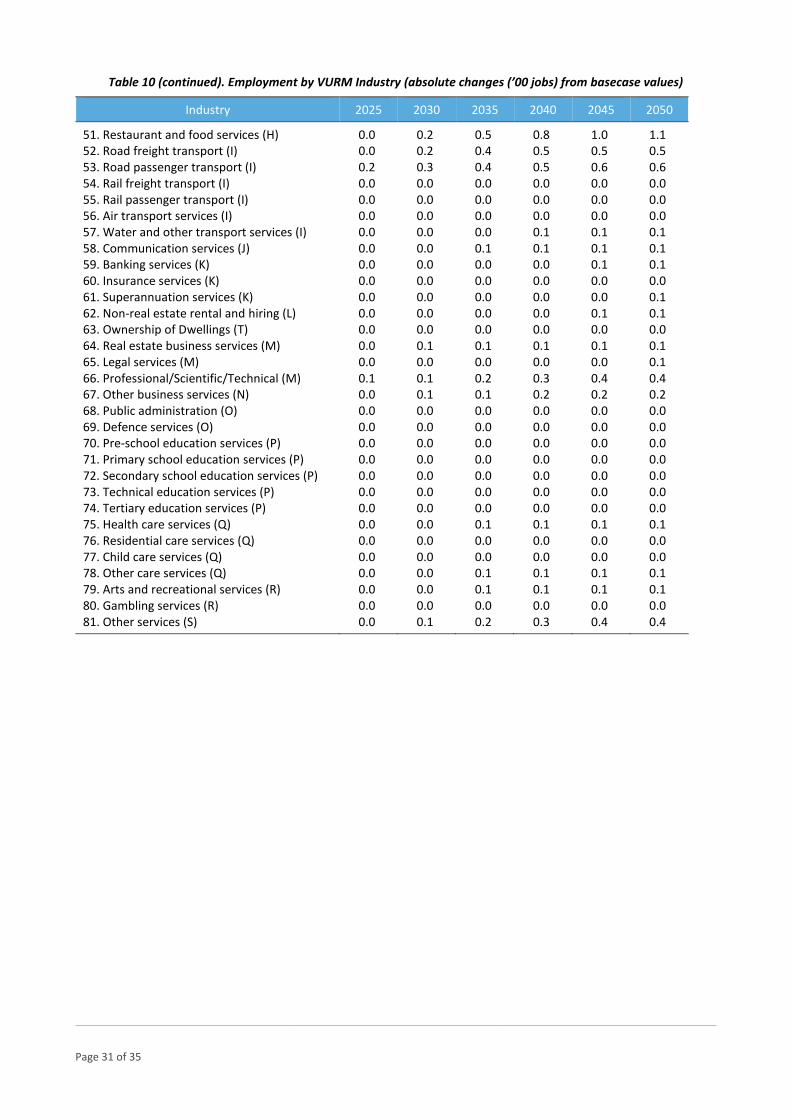
Page 31 of 35

Table 10 (continued). Employment by VURM Industry (absolute changes (’00 jobs) from basecase values)

Industry 2025 2030 2035 2040 2045 2050


Page 32 of 35

Table 11. Employment by VURM Industry (% changes from basecase values)

Industry 2025 2030 2035 2040 2045 2050

1. Sheep and Beef cattle (A) 0.4 1.3 2.2 3.0 3.8 4.5 2. Grains production (A) -0.1 0.6 1.3 2.2 3.1 3.8 3. Dairy cattle (A) 0.5 1.4 2.3 3.3 4.3 5.3 4. Other crop production (A) 0.0 0.2 0.5 0.9 1.3 1.9 5. Sugar cane production (A) 0.0 0.0 0.0 0.0 0.0 0.0 6. Raw cotton and ginning (A) 0.0 0.0 0.0 0.0 0.0 0.0 7. Other Agriculture (A) 0.0 0.1 0.3 0.3 0.4 0.4 8. Fishing, hunting and trapping (A) 0.0 0.0 0.2 0.3 0.3 0.4 9. Forestry and logging (A) 0.0 0.7 1.4 2.1 2.9 3.8 10. Agricultural services (A) 0.1 0.6 1.3 2.0 2.6 3.1 11. Coal mining (B) -0.1 -4.8 -7.6 -8.8 -7.7 -5.5 12. Oil mining (B) 0.0 0.0 0.0 0.0 0.0 0.0 13. Gas mining (B) 0.0 0.0 0.0 0.0 0.0 0.0 14. LNG production (B) 0.0 0.0 0.0 0.0 0.0 0.0 15. Iron ore mining (B) 0.0 0.1 0.3 0.4 0.6 0.7 16. Non-ferrous metal ore mining (B) 0.0 0.3 0.8 1.1 1.3 1.6 17. Non-metallic ore mining (B) 0.0 -0.3 -0.6 -1.0 -1.3 -1.6 18. Exploration and mining services (B) 0.0 0.0 0.1 0.2 0.4 0.5 19. Meat products (C) 0.0 0.4 0.9 1.2 1.3 1.4 20. Dairy products (C) 0.1 0.7 1.4 2.1 2.6 3.1 21. Refined sugar processing (C) 0.0 0.6 1.3 1.6 1.7 1.8 22. Other food products (C) 0.0 0.2 0.4 0.6 0.7 0.8 23. Beverages and tobacco (C) 0.0 0.3 0.8 1.2 1.5 1.8 24. Textiles, clothing and footwear (C) 0.0 0.6 1.7 2.3 2.8 3.1 25. Wood products (C) 0.0 2.6 4.7 6.4 7.7 9.0 26. Pulp and paper products, printing (C) 0.0 1.2 2.7 3.5 3.9 4.1 27. Petroleum refinery products (C) 0.0 0.0 0.0 0.0 0.0 0.0 28. Other chemical products (C) 0.0 0.8 1.6 2.1 2.4 2.5 29. Non-metallic mineral products (C) -0.7 -5.8 -9.9 -12.6 -14.1 -15.3 30. Iron and steel manufacturing (C) 0.0 0.0 0.0 0.0 0.0 0.0 31. Alumina smelting (C) 0.0 0.0 0.0 0.0 0.0 0.0 32. Aluminium refining (C) 0.0 0.0 -0.2 -0.2 -0.1 0.0 33. Other non-ferrous metals (C) 0.0 0.5 1.3 1.8 2.1 2.3 34. Motor vehicles and parts (C) 0.1 0.5 1.2 1.6 1.9 2.2 35. Other transport equipment (C) 0.4 0.2 0.0 0.0 0.0 0.1 36. Other manufacturing (C) 0.1 -1.6 -2.0 -2.4 -2.7 -2.9 37. Electricity – coal (D) 0.0 0.0 0.0 0.0 0.0 0.0 38. Electricity - gas (D) -0.1 2.4 1.8 0.9 0.9 1.0 39. Electricity – hydro (D) -0.1 2.4 1.8 0.9 0.8 1.0 40. Electricity - non-hydro renewable (D) -0.1 2.4 1.8 0.9 0.8 1.0 41. Electricity supply (D) 0.0 -0.1 0.9 1.4 1.9 2.2 42. Gas supply (D) 0.0 -25.7 -30.3 -25.5 -24.6 -24.2 43. Water, waste and drainage (D) 0.1 0.3 0.4 0.6 0.7 0.8 44. Residential construction (E) 0.0 0.3 0.6 0.7 0.7 0.6 45. Non-residential construction (E) 0.8 0.6 0.4 0.6 0.7 0.7 46. Civil engineering (E) 0.8 0.6 0.4 0.6 0.7 0.8 47. Construction services (E) 0.3 0.4 0.5 0.6 0.7 0.7 48. Wholesale trade services (F) 0.1 0.4 0.7 0.9 1.0 1.1 49. Retail trade services (G) 0.0 0.1 0.2 0.4 0.5 0.5 50. Accommodation services (H) 0.0 0.1 0.2 0.3 0.4 0.5

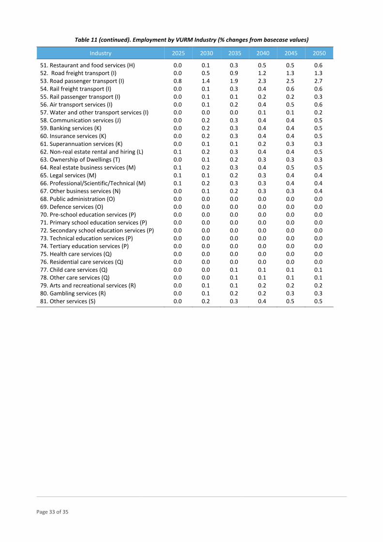
Page 33 of 35

Table 11 (continued). Employment by VURM Industry (% changes from basecase values)

Industry 2025 2030 2035 2040 2045 2050


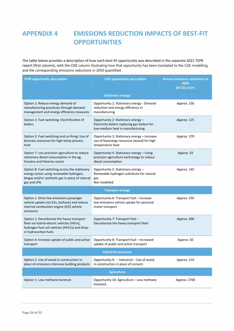
Page 34 of 35

APPENDIX 4 EMISSIONS REDUCTION IMPACTS OF BEST-FIT OPPORTUNITIES

The table below provides a description of how each best-fit opportunity was described in the separate 2021 TEPR report (first column), with the CGE column illustrating how that opportunity has been translated to the CGE modelling,

and the corresponding emissions reductions in 2050 quantified.

TEPR opportunity description CGE opportunity description Annual emissions reductions in 2050

(kt CO2-e/yr)

Stationery energy

Option 1: Reduce energy demand of manufacturing processes through demand management and energy efficiency measures

Opportunity 1: Stationary energy - Demand reduction and energy efficiency in manufacturing

Approx. 230

Option 2: Fuel switching: Electrification of boilers

Opportunity 2: Stationary energy – Electricity boilers replacing gas boilers for low-medium heat in manufacturing

Approx. 125

Option 3: Fuel switching and co-firing: Use of biomass resources for high-temp process heat

Opportunity 3: Stationary energy – Increase use of bioenergy resources (wood) for high temperature heat

Approx. 370

Option 7: Use precision agriculture to reduce stationary diesel consumption in the ag, forestry and fisheries sector

Opportunity 4: Stationary energy – Using precision agriculture technology to reduce diesel consumption

Approx. 55

Option 8: Fuel switching across the stationary energy sector using renewable hydrogen, biogas and/or synthetic gas in place of natural gas and LPG

Opportunity 5: Stationary energy – Renewable hydrogen substitute for natural gas Not modelled

Approx. 145

Transport energy

Option 1: Drive low emissions passenger vehicle uptake (via EVs, biofuels) and reduce internal combustion engine (ICE) vehicle emissions

Opportunity 6: Transport fuel – Increase low emissions vehicle uptake for personal motor transport

Approx. 550

Option 2: Decarbonise the heavy transport fleet via hybrid electric vehicles (HEVs), hydrogen fuel cell vehicles (HFCVs) and drop-in hydrocarbon fuels

Opportunity 7: Transport fuel – Decarbonize the heavy transport fleet

Approx. 690

Option 4: Increase uptake of public and active transport

Opportunity 8: Transport fuel – Increased uptake of public and active transport

Approx. 50

Industrial processes

Option 2: Use of wood in construction in place of emissions intensive building products

Opportunity 9: – Industrial – Use of wood in construction in place of cement.

Approx. 210

Agriculture

Option 1: Low methane livestock Opportunity 10: Agriculture – Low methane livestock.

Approx. 1700

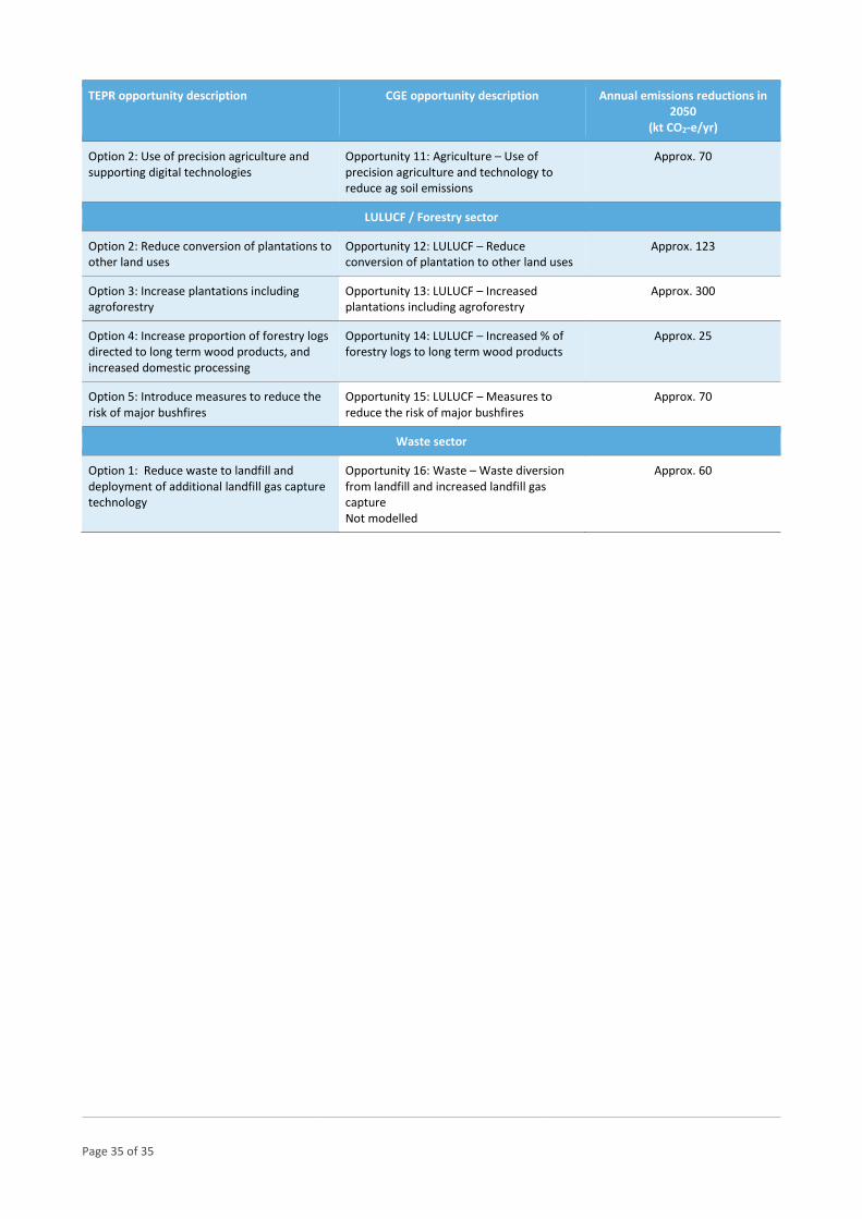
Page 35 of 35

TEPR opportunity description CGE opportunity description Annual emissions reductions in 2050

(kt CO2-e/yr)

Option 2: Use of precision agriculture and supporting digital technologies

Opportunity 11: Agriculture – Use of precision agriculture and technology to reduce ag soil emissions

Approx. 70

LULUCF / Forestry sector

Option 2: Reduce conversion of plantations to other land uses

Opportunity 12: LULUCF – Reduce conversion of plantation to other land uses

Approx. 123

Option 3: Increase plantations including agroforestry

Opportunity 13: LULUCF – Increased plantations including agroforestry

Approx. 300

Option 4: Increase proportion of forestry logs directed to long term wood products, and increased domestic processing

Opportunity 14: LULUCF – Increased % of forestry logs to long term wood products

Approx. 25

Option 5: Introduce measures to reduce the risk of major bushfires

Opportunity 15: LULUCF – Measures to reduce the risk of major bushfires

Approx. 70

Waste sector

Option 1: Reduce waste to landfill and deployment of additional landfill gas capture technology

Opportunity 16: Waste – Waste diversion from landfill and increased landfill gas capture Not modelled

Approx. 60

Documents

2021 Economic Impact Analysis Emissions Pathway Review