Embed Size (px)
Citation preview

2021 SISCER Module 2 Small AreaEstimation:
Lecture 1: Motivation and Survey Sampling
Jon Wakefield
Departments of Statistics and BiostatisticsUniversity of Washington
1 / 83

Outline
OverviewMotivating DataSmoothing and Bayes
Survey SamplingDesign-Based InferenceComplex Sampling Schemes
Use of Auxiliary Information
Discussion
2 / 83

Overview
3 / 83
Motivation
• Small area estimation (SAE) entails estimating characteristics ofinterest for domains, often geographical areas, in which theremay be few or no samples available – “small” refers to thenumber of samples in, and not to the geographical size of, theareas.
• SAE has a long history and a wide variety of methods have beensuggested, from a bewildering range of philosophicalstandpoints.
• Application areas include: epidemiology, public and globalhealth, agriculture, economics, education,...
• The classic text is Rao (2003) which was updated to Rao andMolina (2015).
4 / 83
Data
Examples we discuss include:
• Subnational variation in the under 5 mortality rate (U5MR) in low-and middle-income countries (LMIC).
• Diabetes prevalence in King County health reporting areas.
• Corn and Soy crop yield in Iowa counties.
• Poverty mapping in Spanish regions.
5 / 83

Health and Demographic Indicators
My own research focusses on health/demographic indicators inLMICs:
• Charactering and understanding subnational variation is animportant public health endeavor.
• For example, in the Sustainable Development Goals (SDGs),Goal 3.2 states, “By 2030, end preventable deaths of newbornsand children under 5 years of age, with all countries aiming toreduce neonatal mortality to at least as low as 12 per 1,000 livebirths and under-5 mortality to at least as low as 25 per 1,000live births”.
• Many other indicators have SDG targets, including poverty.
6 / 83
Prevalence Mapping and Geostatistics
• Examination of proportions across space, is known asprevalence mapping – we may map continuously in space, oracross discrete administrative areas – we focus on the latter.
• SAE methods provide one approach to performing prevalencemapping, for administrative areas.
• “The term geostatistics is a short-hand for the collection ofstatistical methods relevant to the analysis of geolocated data, inwhich the aim is to study geographical variation throughout aregion of interest, but the available data are limited toobservations from a finite number of sampled locations.” (Diggleand Giorgi, 2019).
• Model-based geostatistics (MBG) provide another approach toperforming prevalence mapping, over continuous space, thoughthese continuous surfaces can be averaged for area-levelinference.
7 / 83

Characterization of Methods and Approaches
Some important distinctions:
Unit-level versus Area-level ModelingDirect versus Indirect EstimationLinear versus Non-Linear ModelingNo Auxiliary versus Auxiliary DataNon-spatial versus Spatial Mixed ModelingDesign-based versus Model-based InferenceFrequentist versus Bayesian Inference
In general, the lack of information in small samples is compensatedfor by:
• The use of covariates (auxiliary variables) in a regression model.
• Employing smoothing via mixed effects models, perhapsincluding spatial smoothing.
8 / 83

Overview of Short Course
• Data: We consider the common situation in which the availabledata arise from surveys with a complex design.
• A Problem: If small sample sizes in some areas/time periods,there is high instability. In the limit, there may be no data...
• Supplementary Data: On covariates to aid in modeling.• Survey Sampling Methodology: Required for design and
analysis.• Shrinkage and Spatial Smoothing: To reduce instability, use the
totality of data to smooth both locally and globally over space.• Different Approaches to SAE: Both traditional and Bayesian
methods that use spatial smoothing.• Implementation: In R programming environment, using theSUMMER package.
• Visualization: Maps of uncertainty, accompanied withuncertainty, produced using the GIS capabilities of R.
9 / 83

Overview of Short CourseLectures:
• Lecture 1: Motivation and approaches to analyzing complexsurvey data.
• Lecture 2: Mixed effects area-level models and non-spatialsmoothing. MLE and Bayes inference.
• Lecture 3: Mixed effects area-level models and spatialsmoothing.
• Lecture 4: Mixed effects unit-level models and spatial andnon-spatial smoothing.
Methods illustrated in R, in particular using the SUMMER package.
Course website:
http://faculty.washington.edu/jonno/SISCER-SAE.html
10 / 83

My SAE Background
My own interest in SAE:
• Started with work on BRFSS, with local government.
• Moved to estimating subnational estimation of U5MR, neonatalmortality, vaccination, HIV prevalence,... in LMICS.
Details on my research is here:
http://faculty.washington.edu/jonno/space-station.html
11 / 83

Demographic Health Surveys
• Motivation: In many developing world countries, vital registrationis not carried out, so that births and deaths go unreported.
• Objective: To provide reliable estimates of demographic/healthindicators at the (say) Admin1 or Admin2 level1, at which policyinterventions are often carried out.
• We will illustrate using data from Demographic Health Surveys(DHS).
• DHS Program: Typically stratified cluster sampling to collectinformation on population, health, HIV and nutrition; more than300 surveys carried out in over 90 countries, beginning in 1984.
• The Problem: Data are sparse, at the Admin2 level in particular.• SAE: Leverage space-time similarity to construct a Bayesian
smoothing model.
1Admin0 = country level boundaries, Admin1 = first level administrative boundaries(states in US), Admin 2 = second level administrative boundaries (counties in US)
12 / 83

2014 Kenyan DHS
• The 3 most recent Kenya DHSwere carried out in 2003, 2008and 2014.
• The DHS use stratified two-stagecluster sampling. The strataconsist of urban/rural crossedwith geographic administrativestrata.
• In each strata, enumerationareas (EAs ) are selected withprobability proportional to sizeusing a sampling framedeveloped from the most recentcensus.
• In each of the clusters,households are selected. Withineach household, women betweenthe ages of 15 and 49 areinterviewed.
●●●●●●● ●●●●●
●●●●●●●●●●
●●●●●
●●●●●●●●●●●●●●●●●●●●●●●●●
●●●●
●
●
●●
●
●
●
●
●●●
●
●●
●●
●●
●●●●●
● ●●
●
●●
●●
●●
●●●●
●●
●●
●
●●●●
●●●
●
●
●●
●●
●●
●● ●●●●
●●●●●
●●●
●●●●●
●●
●
●●
●●●●
●●
●●
●
●●●●
●●●
●●●●
●●●● ●
●● ●
●● ●●●●
●●●
●●● ●●●●
●
●● ●●●●●
●
● ●
●
●●●●
●●
●●●●●
●● ●
●●
●●
●●
● ●● ●●●●
●●●●●●
●●●●
●
●●
●●●●●●●●●●
●●●●●●●●●●●●●●●●●●●●●●●●
●●
●●
●
●●
●●●
●
●
●
●
●
●●●●●●●●●
● ●
●
●
●
●●
●
●●
●●
●●●
●●
●
●●
●●●●
●●
●● ●
●
●●●●●●
●●
● ●
●
●
●
●
●
●
●
●●
●
●●●●●
●●●●●
●
●●
●●
●
●
●●●●●
●
●●●●●●●●●●●●●
●●
●●●●
●
●
●● ●●●●
●
●●●
●
●
●●
●●●●●●
●●
●●
●●●●
●
●●● ●●●
●
●●●●●
●●●●
●
●
●
●
●
●
●
●
●
●
●
●
●
●
●
●
●●●●●●●
●
●
●
●
●●●●●●●●●
●
●●●●
●
●● ●
●
●●
●
●
●
●●
●
●
●●
●
●● ● ●
●
●
●● ●●
●●●●
● ●●● ●
●●
●●●
●●● ●
●
● ●●
●
● ●● ●
●●● ●●●●●●●● ●
●●●
●● ●●●●●●
●
●●
●
●●
●
●
●
●●●●●●●
●● ●●● ●
●●●●●●
●
●● ●●
●
●●●
●●
●●
●
●●●●
●
●●
●●
●●
●
●
●●
●
●●
●
●
●
●●●
● ●
●●
●
● ●●
●
●●
●
●● ●
●
●●●
●●●●
●
●
●
● ●
●●
●●●
●
●●●
●●
●●
●●●
●
●●
●●●● ●
●●
●●
●●
●●
●
●
●
●
●
●
●●
●●
●
●
●●
●
●●●
●●●●●●●●●
●
●
●
●●
●
●
●
●
●
●
●
●
●
●
●
●
●●
●
●
●
●
●
●
●
●
●
●
●
●
●
●●●●●●●●
●●●●
●
●
●
●●
●
●
●●●●●
●
●
●
●●
●●
●
●●
●
●
●
● ●●●●●●●●
●
●
●
●
● ●
●●●●●
●●
● ●
●●●●
●
●●
●●
●●●●●
●●●
●
●
●●
●
●
●●●●●●●●
●●●● ●
●●
●
●
●●●● ●●●
●●
●
●●
●●●
●●●
●●●●●●
●
●●
●
●●●
●
●
●
●●
●
●●●
●●●
●
●
●●● ●●●
●●
●●●●●●●
●●●
● ●
●
●
●●
●
●●
●
●●
●● ●●
●●
●●●
●●●
●●●●●
●● ●●●●●●●
●●●
●●
●●●
●●●●●
●
●
●●
●●●
●●
●●●
●●●
●
●●●
●●●●●
●●
●
●●●●●●●●
●
●●
●●●
●
●●●●●
●
●●
●
●
●
●
●●
●
●
●
●●
●
●
●
●●
●
●
●
●
●
●
●
●
●●●●●●
●●●
●
●
●
●●
●
●
●
●
●
●●
●●
●●
●●
●
●
●●●●●●●
●
●
●
●
●●
●● ●●
●
●
●
●
●
●
●●
●● ●
●
●
●
●●●●●●
●●●●● ●
●●●●
●
●●
●●●
●●
●
●
●
●
●●●
●●●
●
●
●●●●●
●●●
●
●
●●●●
●
●
●●
●●
●●
●●●●●●● ●
●
●●
●
●
●
●●●●●●
●●●
●
●●●
●
●
●
●●
●
●●
●
●●
●●●●●
●
●
●●●
●
●
●
●●
●
●
●
●
●●
●
●●●●●
●
●
●
●
●●
●
●●
●
●
●●●
●
●●●●●●●●
●●
●●●●●
●●●●
●●●
●●
●●●
●
●●
●●
●
●●●
●●●●●●●●●●●
●
●●
●
●
●
●
●●
●●
●●●●●●● ●●
●
●
● ●●
●●
●
●●●●
●
●
●●●
●●
●
●●
●
●
●
●●●
●
●●●●●●● ●
●
●●
●
●
●●
●
●●
●
●
●
●●●
●
●●
●●
●●
●
●
●
●
●
●
●
●
●●
●
●
●
●
●
●
●
●●●●
●
●
●●
● ●●●●●●● ●●●
●●
● ●●●
●●●●●● ●●
●●
●
● ●●
●●
●●
● ●
●●●
● ● ●●● ●●●●
●●
●●● ●●
●
●●●
●●●●●
●●●
●●●
●●
●
●●●
●
●●●●●
● ●
●
●
●
●
●●
●● ●●
●●●
●
●●
●●
●●● ●●●●●●
●●●●● ●
●●●
●●● ●
●●●● ●
●●●●●●●●●
●●●●●
●●●● ●●
●●●
●
●●
●●
●
●●●●
●●
●●●
● ●●●
●● ●
●
●●
● ●
●●●●
●●●
●●●
●●●●
●●
●●●
●●●●
●●●●
●●●
●●●
●
●
●
●
●
●
●
●
●
●
●
●
●
●●●
●
●
●
●
●
●
●
●
●●
●
●
●
●
●
●●
●
●
●
●
●
●
●
●
●
●
●
●
●
●
●
●
●
●
●
●
●
●
●●
●
●
●
●
●
●
●
●
●
●
●
●
●
●
●
●
●
●●
●
●
●
●
●
●
●
●
●
●
●
●
●
●
●
●
●
●
●
●
●
●
●
●
●
●
●
●
●
●
●
●
●●
●
●
●
●
●
●
●●
●
●
●
●
●
●
●
●
●
●
●
●
●●
●
●
●
●
●
●
●
●
●
●
●
●
●
●
●
●
●
●
●
●
●
●
●
●
●
●●
●
●●
●
●
●
●
●
●
●
●
●
●
●
●
●
●●
●
●
●
●
●
●
●
●
●
●
●
●
●
●
●●
●
●
●
●
●
●
●
●
●
●
●
●
●
●
●
●
●●
●
●●●
●
●
●
●●
●
●
●
●
●
●
●
●
●
●
●
●
●
●
●
●
●
●
●
●
●
●
●
●
●
●
●
●
●
●
●
●●
●
●
●
●
●
●
●
●
●
●
●
●
●
●
●
●●
●
●
●
●
●
●
●
●
●
●
●
●
●
●
●
●
●
●
●
●
●
●
●
●
●
●
●
●
●
●
●
●
●
●●
●
●
●
●
●
●
●
●●
●
●
●
●
●
●
●
●
●
●
●
●
●
●
●
●
●
●
●
●
●
●
●
●
●
●
●
●●
●
●
●
●
●
●●
●
●
●
●
●
●
●
●
●
●
●
●
●
●
●
●
●
●
●
●
●
●
●
●
●
●
●
●
●
●
●
●
●
●●
●
●
●
●
●
●
●●
●
●
●
●
●
●
●
●
●
●
●●
●
●
●
●
●
●
●●●
●
●
●
●
●
●
●
●●
●
●
●
●
●
● ●
●
●
●
●
●
●
●
●
●●
●
●
●
●
●
●
●
●
●
●
●
●
●
●
●
●
●
●
●
●
●
●
●
●
●
●
●
●
●
●
●
●●
●
●
●
●
●
●
●
●
●
●
●
●
●
●
●
●
●
●
●
●
●
● ●
●
●
●
●
●
●
●
●
●
●●
●
●
●
●
●
●
●
●
●
●
●
●
●
●
●
●
●
●
●
●
●
●
●
●
●
●
●
●
●
●
●
●●
●
●
●
●
●
●●
●
●
●
●
●
●
●
●
●
●
●
●
●
●
●
●
●
●
●
●
●
●
●
●
●
●●
●
●
●
●
●
●
●
●
●
●
●
●
● ●
●
●
●
●
●
●
●
●
●
●
●
●
●
●
●
●
●
●
●
●
●
●
●
●
●
●
●
●
●
●
●
●
●
●
●
●
●
● ●
●
●
●
●
●
●
●
●
●
●
●
●
●
●
●
●
●
●
●
●
●
●
●
●
●
●
●
●
●
●
●
●
●
●
●
●
●
●
●
●●● ●
●
●
●
●
●
●
●
●
●
●
●
●
●
●
●
●●
●
●
●
●
●
●
●
●
●
●
●
●
●
●
●
●
●
●
●
●●
●
●
●
●
●
●
●
●
●
●
●
●
●
●
●
●
●
●
●
●
●
●
●
●
●
●
●
●
●
●
●
●
●
●
●
●
●
●
●●
●
●
●
●●
●
●●
●
● ●
●
●
●
●
●
●
●
●
●
●
●
●
●
●
●
●
●●
●
●●
●
●
●●
●
●
●
●
●
●
●
●
●
●
●
●
●
●
●
200320082014
Figure 1: Cluster locations in threeKenya DHS, with county boundaries.
13 / 83

2014 Kenya DHS
• In the 2014 Kenya DHS, thestratification was county (47)and urban/rural (2).
• Nairobi and Mombasa areentirely urban, so there are 92strata in total.
• We have data from a total of1584 EAs across the 92strata. In the second stage,40,300 households aresampled.
• DHS provides sampling(design) weights, assigned toeach individual in the dataset.
id
Baringo
Bomet
Bungoma
Busia
Elgeyo−Marakwet
Embu
Garissa
Homa Bay
Isiolo
Kajiado
Kakamega
Kericho
Kiambu
Kilifi
Kirinyaga
Kisii
Kisumu
Kitui
Kwale
Laikipia
Lamu
Machakos
Makueni
Mandera
Marsabit
Meru
Migori
Mombasa
Murang'a
Nairobi
Nakuru
Nandi
Narok
Nyamira
Nyandarua
Nyeri
Samburu
Siaya
Taita Taveta
Tana River
Tharaka−Nithi
Trans Nzoia
Turkana
Uasin Gishu
Vihiga
Wajir
West Pokot
Figure 2: Counties of Kenya.
14 / 83

Aim: Inference for U5MR over Counties and Years
Figure 3: SAE estimates of under-5 mortality risk, across time, and Kenyancounties. These estimates were obtained using the SUMMER package.
15 / 83

2013 Nigeria DHS
• As a second DHS example, weconsider measles vaccinationrates in Nigeria, from the 2013Nigerian DHS.
• Across African countries, there isgreat variability in the number ofAdmin2 areas.
• In Nigeria, the Admin2 areascorrespond to Local GovernmentAreas (LGAs) and there are 774in total – with such a largenumber there are many LGAswith little/no data.
• There are no clusters in 255LGAs.
Figure 4: Vaccination prevalence forLGAs in Nigeria. LGAs with no dataare in white.
16 / 83

Motivating Example: Diabetes in King County
Arises out of a joint project between Laina Mercer/Jon Wakefield andSeattle and King County Public Health, which lead to the workreported in Song et al. (2016).
Aim we will concentrate on here is to estimate the number of 18 yearsor older individuals with diabetes, by health reporting areas (HRAs) inKing County in 2011.
HRAs are city-based sub-county areas with a total of 48 HRAs inKing County. Some of these are as are a single city, some are agroup of smaller cities, and some are unincorporated areas. Largercities such as Seattle and Bellevue include more than one HRA.
Data are based on the question, “Has a doctor, nurse, or other healthprofessional ever told you that you had diabetes?”, in 2011.
17 / 83

Snoqualmie/North Bend/SkykomishN= 43164
Black Diamond/Enumclaw/SE CountyN= 47803
Bear Creek/Carnation/DuvallN= 64643
Vashon IslandN= 10624 Covington/Maple Valley
N= 54070
Newcastle/Four CreeksN= 28270
West SeattleN= 52689
SammamishN= 45453
ShorelineN= 53030
RedmondN= 53616
BurienN= 48070
KirklandN= 47617
Kent-SEN= 55187
SeaTac/TukwilaN= 46254
NE SeattleN= 67415
Kent-WestN= 27921
Auburn-NorthN= 35235
IssaquahN= 29769
QA/MagnoliaN= 57494
NW SeattleN= 42566
Renton-SouthN= 50711
BallardN= 51822
Auburn-SouthN= 25239
FairwoodN= 23739
Kenmore/LFPN= 34444
Kent-EastN= 35924
Kirkland NorthN= 33564
Bellevue-SouthN= 31100
North SeattleN= 44332
DelridgeN= 30296
Bellevue-NEN= 33096
Merce
r Isle/
Pt C
ities
N= 2
9978Downtown
N= 42610
SE SeattleN= 40305
Des Moines/Normandy Pk
N= 35966
Bothell/WoodinvilleN= 32837
Renton-NorthN= 28608 Renton-East
N= 29871
Bellevue-WestN= 29577
Fed Way-Central/Military Rd
N= 56657
Beacon/Gtown/S.Park
N= 39242
Central SeattleN= 44407
Bellevue-CentralN= 35397
Fed Way-Dash Point/Woodmont
N= 32660
Capitol Hill/E.lakeN= 44740
Fremont/GreenlakeN= 50863
East
Fede
ral W
ay N
= 34
976
North HighlineN= 17400
Health Reporting Areas(HRA)
and 2010 populationKing County, WA
0 2 4 61Miles
N = 2010 population for each HRAData source: Intermin Populationestimates, PHSKC, APDE 1/2012
Produced by: Public Health-Seattle & King County Assessment, Policy Development & Evaluation
Last Modified 08/2012
Auburn, Bellevue, FederalWay, Kent, Renton & Seattle
HRAs are divided into neighborhoods.
Figure 5: Health reporting areas (HRAs) in King County.
18 / 83

Motivating BRFSS Example
Estimates are used for a variety of purposes including summarizationfor the local communities and assessment of health needs.
Analysis and dissemination of place-based disparities is of greatimportance to allow efficient targeting of place-based interventions.
Because of its demographics, King County looks good compared toother areas in the U.S., but some of its disparities are among thelargest of major metro areas.
Estimation is based on Behavioral Risk Factor Surveillance System(BRFSS) data.
The BRFSS is an annual telephone health survey conducted by theCenters for Disease Control and Prevention (CDC) that tracks healthconditions and risk behaviors in the United States and its territoriessince 1984.
19 / 83

Figure 6: Public Health: Seattle and King County website.
20 / 83
S e a ttle
K e nt
B e lle vue
A uburn
K irk la nd
F ede ra l W a y
S ammam is h
B urie n
S hore line
S e a Ta c
T ukw ila
Is s a qua h
B othe ll
K e nm ore
C ov ing ton
D e s Mo ines
S noqua lm ie
Wood inv ille
Map le Va lle y
B la c k D iamond
E num c la w
Merc e r Is la nd
N ewca s tle
N orth B e nd
D uva ll
P a c ific
Med ina
L a ke F ore s t P a rk
A lg ona
N orm a ndy P a rk
R e dmond
C a rna tion
Milton
R e n ton
L ife E x p e c ta n c y C om p a re d toth e Te n L o n g e s t-‐L iv e d C o u n trie sb y C en s u s T ra c t2005 -‐2 009 , K in g C o u n ty WA
D a te : 1 0 /11 /2 011
L e g e n dC IT Y
C a le n d a r Y e a r s A h e a d
S m a ll p opu la tion
C a le n d a r Y e a r s B e h in d
Yea rs be hind or a hea d a re from 2007 .D a ta S ourc es : Inte rna tiona l life ex pe c tanc ies : Ins titute for H e a lth Metric s a nd E va lua tion , U nive rs ity of Wa s h ing tonL oca l life e xpec ta nc y : Wa s h ing ton S ta te D epa rtment of H ea lth,C en ter for H ea lth S ta tis tic s D ea th F ile sA na ly s is a nd p re pa ra tion : A s s es s ment, P o lic y D e ve lopment & E va lua tion ,P ub lic H e a lth ñ S ea ttle & K ing C ounty, 1 0/2011
P repa re d by : A s s es s ment, P o lic y D e ve lopment & E va lua tion
P ro v is io n a l: S u b je c t to R e v is io n
24 to 5 7
10 to 2 3
Z e ro to 9
1 to 1 4
15 to 3 0
31 to 4 2
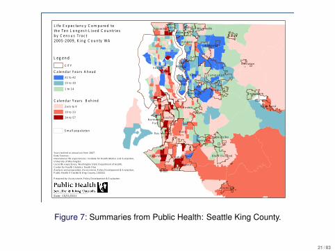
Figure 7: Summaries from Public Health: Seattle King County.
21 / 83

Motivating BRFSS Example
The BRFSS sampling scheme is complex: it uses a disproportionatestratified sampling scheme.
The Design-Wt, is calculated as the product of four terms
Design-Wt = Strat-Wt× 1No-Telephones
× No-Adults
where Strat-Wt is the inverse probability of a “likely” or “unlikely”stratum being selected (stratification based on county and “phonelikelihood”).
Then a raking adjustment. From the documentation, “BRFSS rakesthe design weight to 8 margins (age group by gender, race/ethnicity,education, marital status, tenure, gender by race/ethnicity, age groupby race/ethnicity, phone ownership). If BRFSS includes geographicregions, four additional margins (region, region by age group, regionby gender, region by race/ethnicity) are included.”
22 / 83

Motivating BRFSS Example
Table 1: Summary statistics for population data, and 2011 King CountyBRFSS diabetes data, across health reporting areas.
Mean Std. Dev. Median Min Max TotalPopulation (>18) 31,619 10,107 30,579 8,556 56,755 1,517,712Sample Sizes 62.9 24.3 56.5 20 124 3,020Diabetes Cases 6.3 3.1 6.3 1 15 302Sample Weights 494.3 626.7 280.4 48.0 5,461 1,491,880
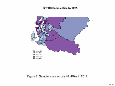
About 35% of the areas have sample sizes less than 50 (CDCrecommended cut-off), so that the diabetes prevalence estimates areunstable in these areas.
We would like to use the totality of the data to aid in estimation in thedata sparse areas.
23 / 83
BRFSS Sample Size by HRA
under 2525 − 5050 − 7575 − 100over 100
Figure 8: Sample sizes across 48 HRAs in 2011.
24 / 83

Observed prevalence by HRA
under 0.050.05 − 0.10.1 − 0.150.15 − 0.2over 0.2
Observed prevalence by HRA
under 0.050.05 − 0.10.1 − 0.150.15 − 0.2over 0.2
Figure 9: Diabetes prevalence by HRAs in 2011. Left: Crude proportions.Right: Horvitz-Thompson weighted estimator.
25 / 83

Two Approaches to Spatial Smoothing
• Model at the area levelusing a discrete spatialmodel. These are the SAEmodels that areimplemented in theSUMMER package.
• Model at the point levelusing a continuous spatialmodel. Model-basedgeostatistics is a popularapproach.
26 / 83

2013 Nigeria DHS• Recall that almost a third of the LGAs in Nigeria have no data
(left plot below).• We fit a discrete spatial model in which the rates in neighboring
areas (as defined by sharing a boundary) are “encouraged” to besimilar (right plot below).
Figure 10: Vaccination prevalences in Nigeria in 2013. Left: Weightedestimates. Right: Estimates from a discrete spatial smoothing model.
27 / 83

Survey Sampling
28 / 83

Outline
Many national surveys employ stratified cluster sampling, also knownas multistage sampling, so that’s where we’d like to get to.
We will discuss:• Simple Random Sampling (SRS).• Stratified SRS.• Cluster sampling.• Multistage sampling.
First, we briefly explain why taking account of the survey design (datacollection process) is important.
29 / 83

Acknowledging the Design: Stratification
Figure 11: In the DHS,stratification is based oncounties (the solid lines) andon a binary urban/ruralvariable (urban indicated inblue, the white is rural).
• Suppose we are interested in theproportion of women aged 20–29who complete secondary education– this is much higher in urban areas
• If we oversample urban areas butignore this when we analyze the datawe will overestimate the fraction ofwomen who complete secondaryeducation, i.e., we will introduce bias.
• Taking into account of thestratification also reduces thevariance of the estimator.
• In the design-based approach toinference, the stratification isaccounted for via design weights.
• In the model-based approach toinference, the stratification isaccounted for in the mean model.
30 / 83

Acknowledging the Design: Cluster Sampling
• The DHS also employs cluster sampling, in which multiple units(individuals) within the same cluster are interviewed.
• Units within the same cluster tend to be more similar than units indifferent clusters, which reduces the information content of theclustered sample, relative to independently sampled units.
• The dependence can be measured via the intraclass correlationcoefficient.
• In the design-based approach to inference, the clustering isaccounted for in the variance calculation that is carried out.
• In the model-based approach to inference, the clustering isaccounted for by including a cluster-specific random effect in themodel.
31 / 83

Modes of Inference
• Surveys can be analyzed using design- and model-basedinference. In this lecture, the former will be focused upon.
• The target of inference are the set of means for areas indexed byi (e.g., Admin2 regions).
• Let yik be the binary indicator on the k -th unit sampled in area i ,for k ∈ Si (the set of selected individuals) and i = 1, . . . ,n.
Design-Based Inference• Labels Si of sampled units
are random.• Responses yik are fixed.• Asymptotic inference,
perhaps using resampling.
Model-Based Inference• Condition on units that are
actually sampled.• Responses Yik are random.• Exact inference, conditional
on model.
32 / 83
Model-Based Inference
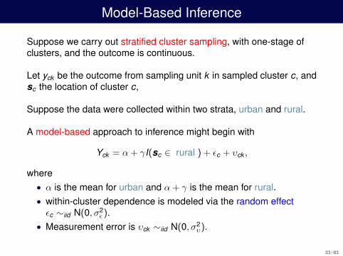
Suppose we carry out stratified cluster sampling, with one-stage ofclusters, and the outcome is continuous.
Let yck be the outcome from sampling unit k in sampled cluster c, andsc the location of cluster c,
Suppose the data were collected within two strata, urban and rural.
A model-based approach to inference might begin with
Yck = α+ γI(sc ∈ rural ) + εc + υck ,
where• α is the mean for urban and α+ γ is the mean for rural.• within-cluster dependence is modeled via the random effectεc ∼iid N(0, σ2
ε ).• Measurement error is υck ∼iid N(0, σ2
υ).
33 / 83

Design-Based Inference
• We will focus on design-based inference: in this approach thepopulation values of the variable of interest:
y1, . . . , yN
are viewed as fixed, while the indices of the individuals who aresampled are random.
• Imagine a population of size N = 4 and we sample n = 2• There are 6 possible samples, with sampled unit indices in red
and non-sampled in blue:y1, y2, y3, y4
y1, y2, y3, y4
y1, y2, y3, y4
y1, y2, y3, y4
y1, y2, y3, y4
y1, y2, y3, y4
• Different designs are possible, and the probabilities we assign toeach sample depend on which is used.
34 / 83

Design-Based Inference
Design-based inference is frequentist, so that properties are basedon hypothetical replications of the data collection process; hence, werequire a formal description of the replication process.
A complex random sample may be:
• Better than a simple random sample (SRS) in the sense ofobtaining the same precision at lower cost, e.g., stratifiedsampling.
• May be worse in the sense of precision, but be requiredlogistically, e.g., cluster sampling.
35 / 83

Probability Samples
Notation for random sampling, in a single population (and notdistinguishing areas):
• N is population size.• n is sample size.• πk is the sampling probability for a unit (which will often
correspond to a person) k , k = 1, . . . ,N.
Random does not mean “equal chance”, but means that the choicedoes not depend on variables/characteristics (either measured orunmeasured), except as explicitly stated via known samplingprobabilities.
For example, in stratified random sampling, the probabilities ofselection differ, in different strata.
36 / 83

Common sampling designs
• Simple random sampling: Select each individual with probabilityπk = n/N.
• Stratified random sampling: Use information on each individualin the population to define strata h, and then sample nh unitsindependently within each stratum.
• Probability-proportional-to-size sampling: Given a variablerelated to the size of the sampling unit, Zk , on each unit in thepopulation, sample with probabilities πk ∝ Zk .
• Cluster sampling: All units in the population are aggregated intolarger units called clusters, known as primary sampling units(PSUs). Clusters are then sampled from this the set of PSUs,with units within these clusters being subsequently sampled.
• Multistage sampling: Stratified cluster sampling, with multiplelevels of clustering.
37 / 83

Probability Samples
• The label probabilitysample is often usedinstead of randomsample.
• Non-probability samplescannot be analyzed withdesign-basedapproaches, becausethere are no πk .
Non-probability sampling approaches include:
• Convenience sampling (e.g., asking forvolunteers). Also known as accidental orhaphazard sampling.
• Purposive (also known as judgmental)sampling in which a researcher usestheir subject knowledge to selectparticipants (e.g, selecting an “average”looking individual).
• Quota sampling in which quotas indifferent groups are satisfied (but unlikestratified sampling, probability samplingis not carried out, for example, theinterviewer may choose friendly lookingpeople!).
38 / 83

Probability Samples: Point Estimation
For design-based inference:
• To obtain an unbiased estimator, every individual k in thepopulation needs to have a non-zero probability πk of beingsampled, k = 1, . . . ,N.
• To carry out inference, this probability πk must be known only forevery individual in the sample.
• So not needed for the unsampled individuals, which is key toimplementation, since we will usually not know the samplingprobabilities for those not sampled.
39 / 83

Probability Samples: Variance Estimation
For design-based inference:
• To obtain a form for the variance of an estimator: for every pair ofunits, k and l , in the sample, there must a non-zero probability ofbeing sampled together, call this probability, πkl for units k and l ,k = 1, . . . ,N, l = 1, . . . ,N, k 6= l .
• The probability πkl must be known for every pair in the sample.
• in practice, these are often approximated, or the variance iscalculated via a resampling technique such as the jackknife.
40 / 83

Inference
• Suppose we are interested in a variable denoted y , with thepopulation values being y1, . . . , yN .
• Random variables will be represented by upper case letters, andconstants by lower case letters.
• Finite population view: We have a population of size N and weare interested in characteristics of this population, for example,the mean:
yU =1N
N∑k=1
yk .
41 / 83

Model-Based Inference
• Infinite population view: The population variables are drawn froma hypothetical distribution, with mean µ.
• In the model-based view, Y1, . . . ,YN are random variables andproperties are defined with respect to p(·); often we say Yk areindependent and identically distributed (iid) from p(·).
• As an estimator of µ, we may take the sample mean:
µ =1n
n∑k=1
Yk .
• µ is a random variable because Y1, . . . ,Yn are each randomvariables.
• Assume Yk are iid observations from a distribution, p(·), withmean µ and variance σ2.
• The sample mean is an unbiased estimator, and has varianceσ2/n.
42 / 83

Model-Based Inference
• Unbiased estimator:
E[µ] = E
[1n
n∑k=1
Yk
]=
1n
n∑k=1
E [Yk ]︸ ︷︷ ︸=µ
=1n
n∑k=1
µ = µ
• Variance:
var(µ) = var
(1n
n∑k=1
Yk
)=︸︷︷︸iid
1n2
n∑k=1
var (Yk )︸ ︷︷ ︸=σ2
=1n2
n∑k=1
σ2 =σ2
n
43 / 83

Model-Based Inference
• The variance σ2 is unknown so we estimate by the unbiasedestimator
s2 =1
n − 1
n∑k=1
(yk − µ)2.
• A 95% asymptotic confidence interval is,
µ± 1.96× s√n.
• In practice, “asymptotic” means that n is sufficiently large that thesampling distribution of µ (i.e., it’s distribution in hypotheticalrepeated samples) is close to normal.
44 / 83

Design-Based Inference
• In the design-based approach to inference the y values aretreated as unknown but fixed.
• To emphasize: the y ’s are not viewed as random variables, so wewrite
y1, . . . , yN ,
and the randomness, with respect to which all procedures areassessed, is associated with the particular sample of individualsthat is selected, call the random set of indices S.
• Minimal reliance on distributional assumptions.• Sometimes referred to as inference under the randomization
distribution.• In general, the procedure for selecting the sample is under the
control of the researcher.
45 / 83

Design-Based Inference
• Define design weights as
wk =1πk.
• The basic estimator is the weighted mean (Horvitz andThompson, 1952; Hajek, 1971)
yU =
∑k∈S wk yk∑
k∈S wk.
• This is an estimator of the finite population mean yU .• So long as the weights are correctly calculated, and the sample
size is not small, this estimator is appealing, though it may havehigh variance, if n is small.
The weighted mean is the basic direct estimator that is thefirst choice for SAE.
46 / 83

Simple Random Sample (SRS)
• The simplest probability sampling technique is simple randomsampling without replacement.
• Suppose we wish to estimate the population mean in a particularpopulation of size N.
• In everyday language: consider a population of size N; a randomsample of size n ≤ N means that any subset of n people fromthe total number N is equally likely to be selected.
47 / 83

Simple Random Sample (SRS)
• We sample n people from N, choosing each personindependently at random and with the same probability of beingchosen:
πk =nN,
k = 1, . . . ,N.• Since sampling without replacement the joint sampling
probabilities are
πkl =nN× n − 1
N − 1for k , l = 1, . . . ,N, k 6= l .
• In this situation:• The sample mean is an unbiased estimator.• The uncertainty, i.e. the variance, of the estimator can be easily
estimated.• Unless n is quite close to N, the uncertainty does not depend on N,
only on n.
48 / 83

The Indices are Random!
• Example: N = 4,n = 2 with SRS. There are 6 possibilities:
{y1, y2}, {y1, y3}, {y1, y4}, {y2, y3}, {y2, y4}, {y3, y4}.
• The random variable describing this design is S, the set ofindices of those selected.
• The sample space of S is
{(1,2), (1,3), (1,4), (2,3) (2,4), (3,4)}
and under SRS, the probability of sampling one of thesepossibilities is 1/6.
• The selection probabilities are
πk = Pr( individual k in sample ) =36=
12
which is of course nN .
• In general, we can work out the selection probabilities withoutenumerating all the possibilities!
49 / 83

Design-Based Inference
• Fundamental idea behind design-based inference: An individualwith a sampling probability of πk can be thought of asrepresenting wk = 1/πk individuals in the population.
• Example: in SRS each person selected represents Nn people.
• The sum of the design weights,∑k∈S
wk = n × Nn
= N,
is the total population.• Sometimes the population size may be unknown and the sum of
the weights provides an unbiased estimator.• In general, examination of the sum of the weights can be useful
as if it far from the population size (if known) then it can beindicative of a problem with the calculation of the weights.
50 / 83

Estimator of yU and Properties under SRS
• The weighted estimator is
yU =
∑k∈S wk yk∑
k∈S wk
=
∑k∈S
Nn yk∑
k∈SNn
=
∑k∈S yk
n= y ,
the sample mean, which is reassuring under SRS!• This is an unbiased estimator, i.e.,
E[yU
]= yU ,
where we average over all possible samples we could havedrawn, i.e., over S.
51 / 83

Unbiasedness
• For many designs:∑
k∈S wk = N so we examine the estimator
yU =1N
∑k∈S
wk yk .
• There’s a neat trick in here, we introduce an indicator randomvariable of selection Ik ∼ Bernoulli(πk ):
E[yU
]= E
[1N
∑k∈S
wk yk
]︸ ︷︷ ︸
S is random in here
= E
[1N
N∑k=1
Ik wk yk
]︸ ︷︷ ︸
Ik are random in here
=1N
N∑k=1
E [Ik ]wk yk =1N
N∑i=1
πk1πk
yk =1N
N∑i=1
yk = yU
52 / 83

Estimator of yU and Properties under SRS
• It can be shown that the variance is
var(y) =(
1− nN
) S2
n, (1)
where,
S2 =1
N − 1
N∑k=1
(yk − yU)2.
• Contrast (1) with the model-based variance which is σ2/n.• The factor
1− nN
is the famous finite population correction (fpc) factor.• Because we are estimating a finite population mean, the greater
the sample size relative to the population size, the moreinformation we have (relatively speaking), and so the smaller thevariance.
• In the limit, if n = N we have no uncertainty, because we knowthe population mean!
53 / 83
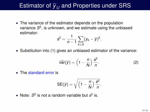
Estimator of yU and Properties under SRS
• The variance of the estimator depends on the populationvariance S2, is unknown, and we estimate using the unbiasedestimator:
s2 =1
n − 1
∑k∈S
(yk − y)2.
• Substitution into (1) gives an unbiased estimator of the variance:
var(y) =(
1− nN
) s2
n. (2)
• The standard error is
SE(y) =
√(1− n
N
) s2
n.
• Note: S2 is not a random variable but s2 is.
54 / 83
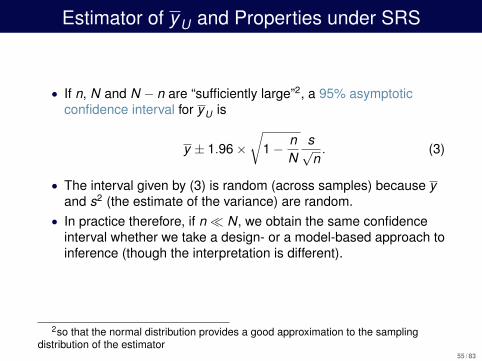
Estimator of yU and Properties under SRS
• If n, N and N − n are “sufficiently large”2, a 95% asymptoticconfidence interval for yU is
y ± 1.96×√
1− nN
s√n. (3)
• The interval given by (3) is random (across samples) because yand s2 (the estimate of the variance) are random.
• In practice therefore, if n� N, we obtain the same confidenceinterval whether we take a design- or a model-based approach toinference (though the interpretation is different).
2so that the normal distribution provides a good approximation to the samplingdistribution of the estimator
55 / 83

Stratified Sampling
• Simple random samples are rarely taken in surveys becausethey are logistically difficult and there are more efficient designsfor gaining the same precision at lower cost.
• Stratified random sampling is one way of increasing precisionand involves dividing the population into groups called strata anddrawing probability samples from within each one, with samplingfrom different strata being carried out independently.
• An important practical consideration of whether stratifiedsampling can be carried out is whether stratum membership isknown for every individual in the population, i.e., we need asampling frame containing the strata variable.
56 / 83

Rationale for Stratified Sampling
Lohr (2010, Section 3.1) provides a good discussion of the benefits ofstratified sampling, we summarize here.
• Protection from the possibility of a “really bad sample”, i.e., veryfew or zero samples in certain stratum giving anunrepresentative sample.
• Obtain known precision required for subgroups (domains) of thepopulation – this is usual for the DHS.
• For example, from the Kenya DHS sampling manual (KenyaNational Bureau of Statistics, 2015):
“The 2014 KDHS was designed to produce representativeestimates for most of the survey indicators at the national level,for urban and rural areas separately, at the regional (formerprovincial) level, and for selected indicators at the county level.”
57 / 83

Rationale for Stratified Sampling
• Flexible since sampling frames can be constructed differently indifferent strata.
• For example, one may carry out different sampling in urban andrural areas.
• More precise estimates can be obtained if stratum can be foundthat are associated with the response of interest, for example,age and gender in studies of human disease.
• In a national study, the most natural form of sampling may bebased on geographical regions.
• Due to the independent sampling in different stratum, varianceestimation is straightforward, as long as within-stratum samplingvariance estimators are available.
58 / 83
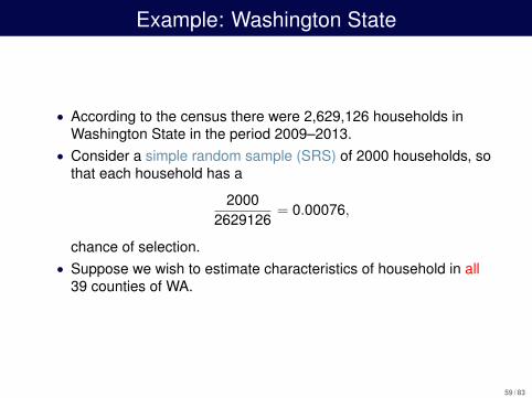
Example: Washington State
• According to the census there were 2,629,126 households inWashington State in the period 2009–2013.
• Consider a simple random sample (SRS) of 2000 households, sothat each household has a
20002629126
= 0.00076,
chance of selection.• Suppose we wish to estimate characteristics of household in all
39 counties of WA.
59 / 83

Example: Washington State
• King (highlighted left) and Garfield (highlighted right) countieshad 802,606 and 970 households so that under SRS we willhave, on average, about 610 households sampled from KingCounty and about 0.74 from Garfield county.
• The probability of having no-one from Garfield County is about22% (binomial experiment), and the probability of having morethan one is about 45%.
• If we took exactly 610 from King and 1 (rounding up) fromGarfield we have an example of proportional allocation, whichwould not be a good idea given the objective here.
• Stratified sampling would allow control of the number of samplesin each county.
60 / 83

Notation
• Stratum levels are denotedh = 1, . . . ,H, so H in total.
• Let N1, . . . ,NH be the knownpopulation totals in the stratumwith
N1 + · · ·+ NH = N,
so that N is the total size of thepopulation.
• In stratified simple randomsampling, the simplest from ofstratified sampling, we take aSRS from each stratum with nh
samples being randomly takenfrom stratum h, so that the totalsample size is
n1 + · · ·+ nH = n.
• We can view stratified SRS as carryingout SRS in each of the H stratum; we letSh represent the probability sample instratum h.
• We also let S refer to the overallprobability sample.
61 / 83

Estimators
• The sampling probabilities for unit k in strata h are
πhk =nh
Nh,
which do not depend on k .• Therefore the design weights are
whk =Nh
nh.
• Note that:
H∑h=1
∑k∈Sh
whk =H∑
h=1
∑k∈Sh
Nh
nh=
H∑h=1
nhNh
nh= N,
so that summing over the weights recovers the population size.
62 / 83

Estimators
• Weighted estimator:
yU =
∑Hh=1
∑k∈Sh
whk yhk∑Hh=1
∑k∈Sh
whk=
H∑h=1
Nh
Nyh
where
yh =
∑k∈Sh
yhk
nh.
• Since we are sampling independently from each stratum usingSRS, we have3
var(yU) =H∑
h=1
(Nh
N
)2(1− nh
Nh
)s2
hnh, (4)
where the within stratum variances are:
s2h =
1nh − 1
∑k∈Sh
(yhk − yh)2.
3using the variance formula for SRS, (2)63 / 83

Weighted Estimation
Recall: The weight wk can be thought of as the number of people inthe population represented by sampled person k .
Example 1: Simple Random SamplingSuppose an area contains 1000 people:• Using simple random sampling (SRS), 100 people are sampled.• Sampled individuals have weight wk = 1/πk = 1000/100 = 10.
Example 2: Stratified Simple Random SamplingSuppose an area contains 1000 people, 200 urban and 800 rural.• Using stratified SRS, 50 urban and 50 rural individuals are
sampled.• Urban sampled individuals have weight
wk = 1/πk = 200/50 = 4.• Rural sampled individuals have weight
wk = 1/πk = 800/50 = 16.
64 / 83

Weighted Estimation
Example 2: Stratified Simple Random SamplingSuppose an area contains 1000 people, 200 urban and 800 rural.• Urban risk = 0.1.• Rural risk = 0.2.• True risk = 0.18.
Take a stratified SRS, 50 urban and 50 rural individuals sampled:
• Urban sampled individuals have weight 4; 5 cases out of 50.• Rural sampled individuals have weight 16; 10 cases out of 50.• Simple mean is 15/100 = 0.15 6= 0.18.• Weighted mean is
4× 5 + 16× 104× 50 + 16× 50
=1801000
= 0.18.
65 / 83

Motivation for Cluster Sampling
For logistical reasons, cluster sampling is an extremely commondesign that is often used for government surveys.
Two main reasons for the use of cluster sampling:• A sampling frame for the population of interest does not exist,
i.e., no list of population units.• The population units have a large geographical spread and so
direct sampling is not logistically feasible to implement forin-person interviews.
• It is far more cost effective (in terms of travel costs, etc.) tocluster sample.
66 / 83

Terminology
• In single-stage cluster sampling or one-stage cluster sampling,the population is grouped into subpopulations (as with stratifiedsampling) and a probability sample of these clusters is taken,and every unit within the selected clusters is surveyed.
• In one-stage cluster sampling either all or none of the elementsthat compose a cluster (PSU) are in the sample.
• The subpopulations are known as clusters or primary samplingunits (PSUs).
• In two-stage cluster sampling, rather than sample all units withina PSU, a further cluster sample is taken; the possible groups toselect within clusters are known as secondary sampling units(SSUs).
• This can clearly be extended to multistage cluster sampling.
67 / 83

Differences Between Cluster and Stratified sampling
Stratified Random Sampling One-Stage Cluster SamplingA sample is taken from every Observe all elements only within thestratum sampled clustersVariance of estimate of yU The cluster is the sampling unit and thedepends on within strata variability more clusters sampled the smaller the
variance – which depends primarily onbetween cluster means
For greatest precision, we want low For greatest precision, high within-clusterwithin-strata variability but large variability and similar cluster means.between-strata variabilityPrecision generally better than SRS Precision generally worse than SRS
68 / 83

Heterogeneity
• The reason that cluster sampling loses efficiency over SRS isthat within clusters we only gain partial information fromadditional sampling within the same cluster, since within clusterstwo individuals tend to be more similar than two individuals withindifferent clusters.
• The similarity of elements within clusters is due to unobserved(or unmodeled) variables.
• The design effect (deff) is often to summarize the effect on thevariance of the design:
deff =Variance of estimator under designVariance of estimator under SRS
,
where in the denominator we use the same number ofobservations as in the complex design in the numerator.
69 / 83

Estimation for One-Stage Cluster Sampling
• We suppose that a SRS of n PSUs is taken.• The probability of sampling a PSU is n/N, and since all the
SSUs are sampled in each selected PSU we have selectionprobabilities and design weights:
πik = Pr( SSU k in cluster i is selected ) =nN
wik = Design weight for SSU k in cluster i =Nn.
Let S represent the set of sampled clusters.
70 / 83
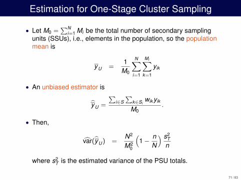
Estimation for One-Stage Cluster Sampling
• Let M0 =∑N
i=1 Mi be the total number of secondary samplingunits (SSUs), i.e., elements in the population, so the populationmean is
yU =1
M0
N∑i=1
Mi∑k=1
yik
• An unbiased estimator is
yU =
∑i∈S∑
k∈Siwik yik
M0.
• Then,
var(yU) =N2
M20
(1− n
N
) s2Tn
where s2T is the estimated variance of the PSU totals.
71 / 83

Two-Stage Cluster Sampling with Equal-ProbabilitySampling
It may be wasteful to measure all SSUs in the selected PSUs, sincethe units may be very similar and so there are diminishing returns onthe amount of information we obtain.
We discuss the equal-probability two stage cluster design:
1. Select a SRS of n PSUs from the population of N PSUs.2. Select a SRS of mi SSUs from each selected PSU, the
probability sample collected will be denoted Si .
72 / 83
Two-Stage Cluster Sampling Weights
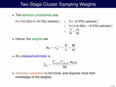
• The selection probabilities are:
Pr( k -th SSU in i-th PSU selected ) = Pr( i-th PSU selected )
× Pr( k -th SSU | i-th PSU selected )
=nN× mi
Mi
• Hence, the weights are
wik = π−1ik =
Nn× Mi
mi.
• An unbiased estimator is
yU =
∑i∈S∑
k∈Siwik yik
M0.
• Variance calculation is not trivial, and requires more thanknowledge of the weights.
73 / 83

Variance Estimation for Two-Stage Cluster Sampling
• In contrast to one-stage cluster sampling we have toacknowledge the uncertainty in both stages of sampling; inone-stage cluster sampling the totals ti are known in the sampledPSUs, whereas in two stage sampling we have estimates ti .
• In Lohr (2010, Chapter 6) it is shown that
var(yU) =1
M20
N2(
1− nN
) s2Tn︸ ︷︷ ︸
One-stage cluster variance
+Nn
∑i∈S
(1− mi
Mi
)M2
is2
imi︸ ︷︷ ︸
Two-stage cluster variance
(5)
where• s2
T is the estimated variance of the cluster totals,• s2
i is the estimated variance within the i-th PSU.
• In most software packages, the second term in (5) is ignored,since it is small when compared to the first term, when N is large.
74 / 83

The Jackknife
• The jackknife is a very general technique for calculating thevariance of an estimator.
• The basic idea is to delete portions of the data, and then fit themodel on the remainder – if one repeats this process for differentportions, one can empirically obtain the distribution of theestimator.
• The key is to select the carefully select the portion of the data sothat the design is respected.
• We describe in the context of multistage cluster sampling.• Observations within a PSU should be kept together when
constructing the data portions, which preserves the dependenceamong observations in the same PSU.
75 / 83

The Jackknife for Multistage Cluster Sampling
• Assume we have H strata and nh PSUs in strata h, and assumePSUs are chosen with replacement.
• To apply the jackknife, delete one PSU at a time.• Let µ(hi) be the estimator when PSU i of stratum h is omitted.• To calculate µ(hi) we define a new weight variable:
wk(hi) =
wk(hi) if observation k is not in stratum h0 if observation k is in PSU i of stratum h
nhnh−1 wk if observation k is not in PSU i but in stratum h
Then we can use the weights wk(hi) to calculate µ(hi) and
VJK(µ) =H∑
h=1
nh − 1nh
nh∑i=1
(µ(hi) − µ)2.
76 / 83

Multistage Sampling in the DHS
• A common design in national surveys is multistage sampling, inwhich cluster sampling is carried out within strata.
• DHS Program: Typically, 2-stage stratified cluster sampling:• Strata are urban/rural and region.• Enumeration Areas (EAs) sampled within strata (PSUs).• Households within EAs (SSUs).
• Weighted estimators are used and a common approach tovariance estimation is the jackknife (Pedersen and Liu, 2012)
• In later lectures, we will show how model-based inference can becarried out for the DHS.
77 / 83
Use of Auxiliary Information
78 / 83

Synthetic EstimatesMany approaches have been suggested to obtain estimators withgreater precision – we discuss three, to give a flavor.
We consider estimation of a generic mean in area i .
• Synthetic Estimator:
Y syni =
1Ni
Ni∑k=1
x Tik B,
where
B =
n∑i=1
∑k∈Si
wik x Tik x ik
−1n∑
i=1
∑k∈Si
wik x Tik yik .
• Note: Covariates needed for all of population.• Assumes regression model is appropriate for all areas.• In general gives high precision estimates – variance is O(1/n),
but possibility of large bias.79 / 83
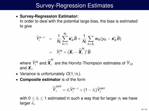
Survey-Regression Estimates
• Survey-Regression Estimator:In order to deal with the potential large bias, the bias is estimatedto give
Y s−ri =
1Ni
Ni∑k=1
x Tik B +
1Ni
∑k∈Si
wik (yik − x Tik B)
= Y hti + (X i − X
ht
i )TB
where Y hti and X
ht
i are the Horvitz-Thompson estimates of Y Uiand X i .
• Variance is unfortunately O(1/ni).• Composite estimator is of the form
Ycom
i = δi Y s−ri + (1− δi)Y
syni
with 0 ≤ δi ≤ 1 estimated in such a way that for larger ni we havelarger δi .
80 / 83

Discussion
81 / 83

Discussion
• SAE is often based on samples collected under a complexdesign, and if this case one must account for the design in theanalysis.
• Direct (weighted) estimates are the starting point for analysis,and will be suitable, if the sample size is sufficiently large.
• Variance estimation that accounts for the design has been atopic of much research.
• However, for the major designs (e.g., SRS, stratified SRS, clustersampling, multistage sampling), weighted estimates and theirvariances are available within all the major statistical packages.
82 / 83

Discussion
• When the variance is large, because of small sample sizes, wewould like to use smoothing methods, with Bayes being aconvenient way to do this – this is the topic of the next lecture.
• We will also consider how covariate information can be used.
• The majority of survey sampling texts take a design-based viewof inference – this is a different paradigm to model-basedinference, for which most spatial statistical models weredeveloped!
• Later we will see how spatial methods can incorporate the surveydesign.
83 / 83

References
Diggle, P. J. and Giorgi, E. (2019). Model-based Geostatistics forGlobal Public Health: Methods and Applications. Chapman andHall/CRC.
Hajek, J. (1971). Discussion of, “An essay on the logical foundationsof survey sampling, part I”, by D. Basu. In V. Godambe andD. Sprott, editors, Foundations of Statistical Inference. Holt,Rinehart and Winston, Toronto.
Horvitz, D. and Thompson, D. (1952). A generalization of samplingwithout replacement from a finite universe. Journal of the AmericanStatistical Association, 47, 663–685.
Kenya National Bureau of Statistics (2015). Kenya Demographic andHealth Survey 2014. Technical report, Kenya National Bureau ofStatistics.
Lohr, S. (2010). Sampling: Design and Analysis, Second Edition.Brooks/Cole Cengage Learning, Boston.
Pedersen, J. and Liu, J. (2012). Child mortality estimation:Appropriate time periods for child mortality estimates from full birthhistories. PLoS Medicine, 9, e1001289.
Rao, J. (2003). Small Area Estimation. John Wiley, New York.83 / 83

Rao, J. and Molina, I. (2015). Small Area Estimation, Second Edition.John Wiley, New York.
Song, L., Mercer, L., Wakefield, J., Laurent, A., and Solet, D. (2016).Peer reviewed: Using small-area estimation to calculate theprevalence of smoking by subcounty geographic areas in KingCounty, Washington, behavioral risk factor surveillance system,2009–2013. Preventing Chronic Disease, 13.
83 / 83


![Thinking mathematically: estimation€¦ · Web viewTI-AIE Thinking mathematically: estimation This publication forms part of the Open University module [module code and title]](https://img.pdfslide.net/doc/110x75/5f1063f17e708231d448e01a/thinking-mathematically-estimation-web-view-ti-aie-thinking-mathematically-estimation.jpg)