21 Polar and ice-edge marine systems - LTERpal.lternet.edu/docs/bibliography/Public/245lterc.pdf · 21 Polar and ice-edge marine systems Andrew Clarke, ... Fishing outside Southern

21 � Polar and ice-edge marine systems

Andrew Clarke, Andrew S. Brierley, Colin M. Harris, Dan Lubin and Raymond C. Smith

INTRODUCTION

Cold, seasonal and dominated by ice, the two polar regions

are similar in many ways. Oceanographically, however,

they are very different. The Arctic is a deep basin sur-

rounded almost completely by extensive shallow contin-

ental shelves and continental land masses. Large river

systems (Chapter 2) discharge significant volumes of fresh

water and sediment into the Arctic basin, some of them

carrying substantial pollution, and exchange with the

Pacific and Atlantic Oceans is highly constrained. In direct

contrast, the Antarctic is a single isolated land mass sur-

rounded on all sides by a deep ocean contiguous with the

three great ocean basins (Fig. 21.1).

Climate change has been identified as the key envir-

onmental trend in both polar regions, with the most likely

effect in the marine environment being mediated through

changes in sea-ice dynamics (Clarke & Harris 2003)

(Table 21.1). The polar regions play a critical role in the

Aquatic Ecosystems, ed. N. Polunin. Published by Cambridge University Press. ª Foundation for Environmental Conservation 2008.

319

regulation of global climate, and it is expected that future

climatic shifts will be particularly pronounced at high

latitudes (IPCC [Intergovernmental Panel on Climate

Change] 2001a). The precise patterns of change and the

feedbacks that influence these are, however, poorly

understood and our ability to predict the future is greatly

limited by this uncertainty.

Major Arctic trends

Current expectations are that the Arctic region will be the

first to experience substantial climate change, with a pos-

sible rise in average surface air temperature of 4–5 �C by

the middle of this century (Stouffer et al. 1989; Manabe

et al. 1991; IPCC 2001a). Increases in spring and summer

air temperatures have already been detected (Martin et al.

1997), and both thinning and a decrease in spatial extent

have been described for Arctic sea ice (Maslanik et al.

1996; Parkinson et al. 1999; Wadhams & Davis 2000;

Rothrock et al. 2003). The IPCC (2001a) concluded that

average Arctic sea-ice extents had declined by 15% in

summer and 8% in spring, and there is some evidence that

the rate of reduction may have been accelerating in recent

years ( Johannessen et al. 1995).

Reductions in sea-ice cover will have important

oceanographic consequences, driven by changes in air–sea

exchanges, irradiance and water-column stability. There

are also probable impacts on Arctic marine biota at all levels

in the food web (Tynan & DeMaster 1997). In addition,

there has been a direct impact on the Arctic marine system

through fishing and hunting. Many Arctic marine mam-

mals have been overexploited in the past (Pagnan 2000)

with many species still globally endangered. New devel-

opments in fishery technology have also increased the scale

of fish catches in the Arctic, and overharvesting has led to

the collapse of stocks of several species (Pagnan 2000).

Human activities have also had a major influence on the

Arctic through the dissemination of pollution from both

local and global sources (AMAP [Arctic Monitoring and

Assessment Programme] 1998). These contaminants

include persistent organic pollutants, heavy metals, acid

rain, sulphur deposition, hydrocarbons from oil and gas

extraction, and radioactivity. Industrial chlorinated

hydrocarbons have also led to the depletion of stratospheric

ozone over the Arctic (Pyle 2000). This pattern of pollution

reflects both the long-distance dispersal from industry at

lower latitudes and the topography of the Arctic as a basin

almost completely surrounded by continental land masses.

A t l an t i cOcean

A t l an t i c

Ocean

Pac i f i c

RussiaKaraSea

BeaufortSea

Alaska(USA) South

America

SouthGeorgla

Canada

South Africa

AmundsenSea

Australia

Ocean

S o u t h e r n O c e a n

NewZealand

40ºS

Pa

c i f i cO

c e a n

Ind i anO

ce

an

90ºE90ºWANTARCTICA

0º

180º

WeddellSea

ARCTICOCEAN

180º

Iceland

40ºN

FramStrait

Sw

eden

BeringSea

ChukchiSea

E.Siberian Sea

RossSea

Antarctic Peninsula

Scot

ia

Sea

SouthShetlandIslands

Is.Kerguelen

Mean positions of the polar frost

CCAMLR boundary

BellingshausenSea

60ºS

Green

land

(Den

mar

k)

Ocean

LaptevSea

BarentsSea

HudsonBay

Nor

way

UK

0º

60ºN

80ºS

Finland

90ºW 90ºE

S ou t he rn

Fig. 21.1. The Arctic and Antarctic, showing the differences

in topography and connections to lower latitude oceans. In

the Antarctic, the dotted line shows the mean position of the

Antarctic Polar Front. CCAMLR, Commission for the

Conservation of Antarctic Marine Living Resources.

320 A. CLARKE ET AL.

Major Antarctic trends

Environmental trends in the Antarctic are similar in many

ways to the Arctic, with climate change, stratospheric

ozone depletion and fishing pressure being the most

important. Pollution is currently much less of a threat to

the Southern Ocean than in the Arctic (Clarke & Harris

2003). It is, however, difficult to detect any clear envir-

onmental trends for the Antarctic marine ecosystem as a

whole, although there are localized trends in some areas.

The Antarctic Peninsula is warming rapidly, but the

Antarctic continent itself shows no spatially consistent

trend (King 1994). The reason for this difference is not

clear, though the climate of the Antarctic Peninsula area is

highly sensitive to the complex feedbacks between

atmosphere, oceans and sea ice, and is strongly influenced

by climatic variations in the subtropical and tropical

Pacific Ocean (King & Harangozo 1998; Yuan & Martinson

2000, 2001).

In recent years, a reduction in sea ice in some areas

( Jacobs & Comiso 1993) has been balanced by an increase

in others, and there is currently no evidence for a decline

in overall sea-ice extent around Antarctica (Zwally et al.

2002). The Amundsen and Bellingshausen Seas have

shown a significant decrease in sea ice, however, and this

may be related to the regional climate warming of the

Antarctic Peninsula. In the western Antarctic Peninsula

region, sea-ice extent has decreased with consequent

impact on all trophic levels of the marine ecosystem (Smith

et al. 2003a, b). This may offer a valuable analogue for

future changes elsewhere in polar regions.

Like the Arctic, the Southern Ocean living resources

have a long history of human exploitation. Following the

exploratory voyage of Captain James Cook in the eighteenth

century, a fishery for southern fur seal (Arctocephalus gazella)

developed rapidly. By 1822, a period of only 35 years,

the industry collapsed (Bonner 1982), and exploitation

shifted to the great whales. By the late 1960s, whale stocks

Table 21.1. Summary of major environmental trends and principal threats to polar marine ecosystems

Category Threats and trends

Arctic

Environmental trends (1) Some evidence for significant change in sea-ice extent and thickness in Arctic Ocean,

though spatial patterns of change non-uniform

(2) Moderate ozone depletion

(3) Fishing has severely depleted stocks of fish and some marine mammals

Threats (long-term) (1) Climate change, with consequent impacts on sea ice, hydrological cycle and UV-B flux

Threats (short-term) (1) Fishing impact

(2) Mineral extraction (especially pollution impacts)

Antarctic

Environmental trends (1) Significant atmosphere warming in Antarctic peninsula, but not over continent

(2) Significant depletion of springtime ozone levels since c.1970, with consequent increase in

UV-B flux. Believed to have peaked, with improvement expected over next 25 years

(3) Significant decrease in extent of winter sea ice in Bellingshausen/Amundsen seas, but not

in other sectors, since advent of satellite observations. Longer-term trends contentious

(4) Southern Ocean fishery has severely depleted stocks of some fish, and some marine

mammals. Recovery of fish and whale stocks slow; southern fur seal stock recovery rapid.

Fishing outside Southern Ocean has by-catch impact on some seabirds that breed south

of the Antarctic Polar Front, especially albatrosses and larger petrels

Threats (long-term) (1) Climate change in Antarctic peninsula area, with consequent impacts on sea ice

Threats (short-term) (1) Illegal, unreported and unregulated (IUU) fishing activity, both in terms of impact on

exploited stocks and on seabird by-catch

Source: From Clarke and Harris (2003).

Polar and ice-edge marine systems 321

had been severely depleted and attention switched to finfish,

the exploitation of which continues today, together with a

fishery for Antarctic krill (Euphausia superba).

In this chapter, the predominant environmental trends

and threats identified by Clarke and Harris (2003) are used

as a basis for predicting likely states of the two polar

marine environments in 2025. Climate, ozone, sea ice and

fishing are separately addressed, and the chapter concludes

with a discussion of how human influences might be

mitigated by regulatory actions.

CLIMATE

The future of both the Arctic and Antarctic marine eco-

systems is linked very closely with climate change. During

the past decade, the polar regions have exhibited many of

the first unmistakable signs of climate warming, and the

ecological manifestations of this warming are magnified by

its dramatic impact on sea-ice cover. Observationally, cli-

mate warming throughout much of the Arctic, and in

Antarctic locations particularly relevant for marine ecol-

ogy, is well established (e.g. Stammerjohn & Smith 1996;

Rigor et al. 2000). Satellite passive microwave observations

have documented the significant retreat of Arctic sea-ice

cover, along with a slight but statistically significant

increase in Antarctic sea-ice cover when averaged over the

entire Southern Ocean (Cavalieri et al. 1997; Johannessen

et al. 1999; Zwally et al. 2002). These trends in sea-ice

cover in both hemispheres are consistent with predictions

from global climate model (GCM) simulations (Cavalieri

et al. 1997; discussed below). The sea-ice retreat in the

western Antarctic Peninsula region has not yet been

reproduced in GCM simulations, although a plausible

mechanism was proposed by Thompson and Solomon

(2002). The mechanisms behind high-latitude climate

warming are dynamically very complex, but are very likely

to have an anthropogenic component.

Feedbacks in the polar climate system

For many years, high-latitude climate warming has

been expected as a result of classical climate-feedback

mechanisms involving surface albedo (the ratio of reflected

to incident electromagnetic radiation), solar and terrestrial

radiation, and cloud cover (Crane & Barry 1984; Somerville

& Remer 1984; Ledley 1993; Curry & Webster 1999). In

the ice–albedo feedback, which should be significant at

temperatures close to the triple-point of water, a warming

induces a localized melting of snow or ice, which thereby

reduces the surface albedo. This reduced albedo leads to

enhanced absorption of short-wave radiation by the sur-

face, which thus accelerates the melting rate and further

decreases the albedo. The result is a reduction in short-

wave radiation backscattered to space by the Earth–

atmosphere system, a concomitant increase in shortwave

absorption by the surface and a decrease in snow/ice cover,

which together constitute a strong positive feedback to

climate warming. A warmer climate may also allow the

atmosphere to hold more water vapour, and this water

vapour will partially close infrared windows (the wave-

length ranges over which the atmosphere is largely trans-

parent to radiation) such that atmospheric long-wave

emission warms the surface to a greater extent. This water-

vapour feedback is another potentially important positive

feedback at high latitudes (Curry et al. 1995). There is also

a general cloud–radiation feedback (Curry & Webster

1999), through which changes in atmospheric precipitable

water force changes in cloud amount, vertical distribution,

optical depth, thermodynamic phase, effective droplet

radius and ice particle size and temperature. The present

consensus is that the net effect of these feedback mech-

anisms should be positive at high latitudes, although

analysis of trends in satellite temperature data has chal-

lenged this conclusion (Wang & Key 2003). In contrast to

these positive feedbacks, a negative feedback can arise if

there is increasing precipitation on sea ice resulting from a

warming atmosphere containing more moisture (Ledley

1993). In this scenario, the snow cover build-up increases

the surface albedo, thus decreasing the absorbed short-

wave radiation, and also decreases the turbulent energy

flux from the ocean to the atmosphere.

The Arctic Oscillation

Recent research in atmospheric dynamics has introduced

a new perspective on high-latitude climate change.

Thompson and Wallace (1998) identified the Arctic

Oscillation (AO), a persistent mode of variability in

atmospheric circulation, as a major regulator of Arctic

surface temperature. In its simplest conception, the AO

can be thought of as a see-saw in sea-level pressure,

alternately rising over the central Arctic Ocean and then in

a sub-Arctic belt ranging from southern Alaska to Europe.

The AO and the North Atlantic Oscillation (NAO) index

which has been known for several decades are often con-

sidered part of the same dynamic phenomenon, the


Northern Annular Mode (NAM), although this view

remains somewhat controversial. Physically, the NAM is

manifest as an oscillation in the strength of counter-

clockwise zonal atmospheric flow at temperate and high

latitudes. Two important aspects of annular modes are

relevant to climate change. Firstly, they do not necessarily

vary in a periodic way; they can vary both monthly

and annually. Secondly, annular modes are easily excited

by external physical forcing such as atmospheric warming.

The interaction between the AO and climate is

described by the AO index, defined as the leading principal

component of the wintertime (November–April) monthly

mean sea-level pressure anomaly field poleward of 20�N.

In the positive phase of this oscillation (high AO index),

stronger westerlies isolate colder air to the north, allowing

Arctic temperatures at many locations to become warmer.

In the negative phase (low AO index), there are relatively

weak westerly winds, and colder air is allowed to spill out

further south at most longitudes. During the past two

decades, there has been a shift toward a positive phase in

the NAM, and this may be the direct cause of much of the

observed Arctic warming (Thompson & Wallace 2001).

In addition to this direct effect on Arctic surface air

temperatures, the AO has been dynamically linked to Arctic

sea-ice concentrations (Rigor et al. 2002). During low AO

index conditions there is a substantial clockwise circulation

in the Beaufort Gyre, which confines much sea ice into the

colder central Arctic where it tends to thicken. During high

AO index conditions this circulation weakens, ice residence

time in the central Arctic is reduced, and there is a more

rapid passage of ice through the Fram Strait into the North

Atlantic. The AO thus has both thermodynamic and direct

dynamic impacts on Arctic sea-ice cover.

Although the NAM mechanism would appear to lessen

the role of direct greenhouse and similar forcings in high-

latitude warming, these anthropogenic factors may still have

a prominent indirect role. Current GCM simulations are

beginning to reproduce the NAM (Moritz et al. 2002), and

some models suggest that a strengthening of the AO may

result from anthropogenic greenhouse forcing (Shindell

et al. 1999).

The Southern Annular Mode

and Antarctic ozone

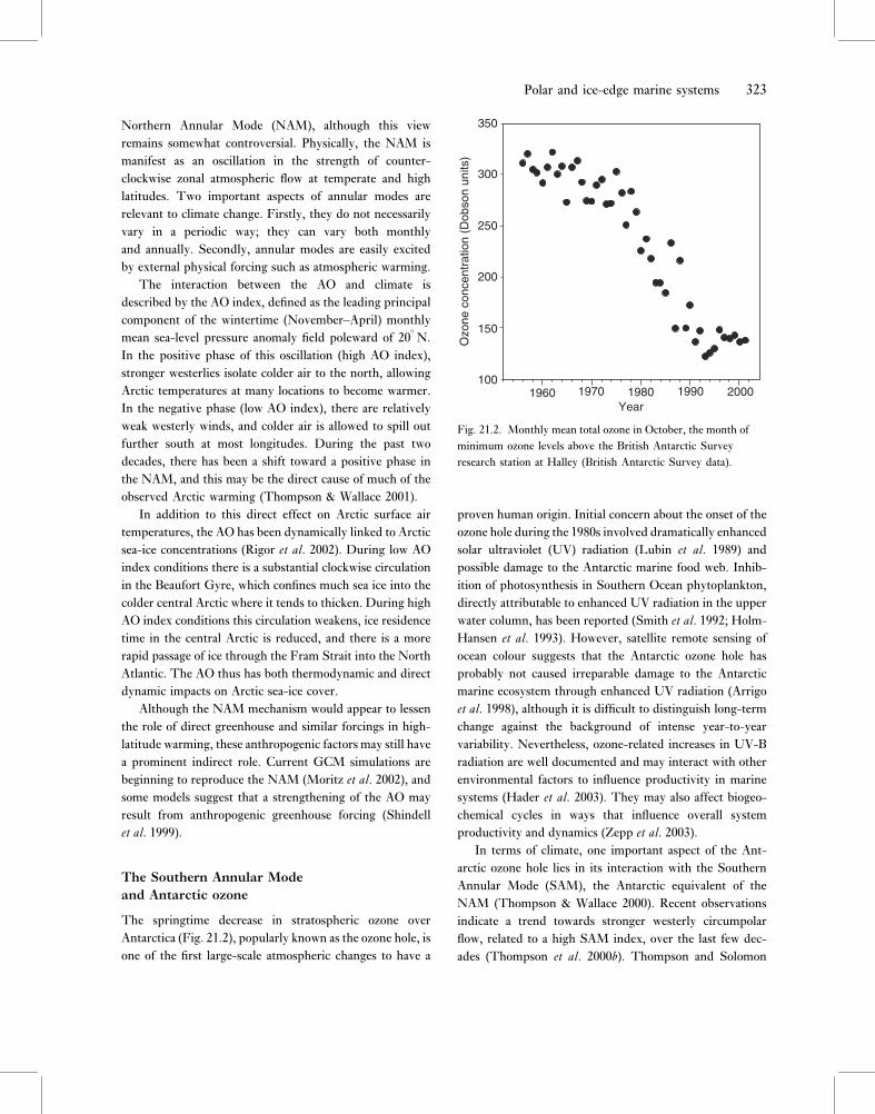
The springtime decrease in stratospheric ozone over

Antarctica (Fig. 21.2), popularly known as the ozone hole, is

one of the first large-scale atmospheric changes to have a

proven human origin. Initial concern about the onset of the

ozone hole during the 1980s involved dramatically enhanced

solar ultraviolet (UV) radiation (Lubin et al. 1989) and

possible damage to the Antarctic marine food web. Inhib-

ition of photosynthesis in Southern Ocean phytoplankton,

directly attributable to enhanced UV radiation in the upper

water column, has been reported (Smith et al. 1992; Holm-

Hansen et al. 1993). However, satellite remote sensing of

ocean colour suggests that the Antarctic ozone hole has

probably not caused irreparable damage to the Antarctic

marine ecosystem through enhanced UV radiation (Arrigo

et al. 1998), although it is difficult to distinguish long-term

change against the background of intense year-to-year

variability. Nevertheless, ozone-related increases in UV-B

radiation are well documented and may interact with other

environmental factors to influence productivity in marine

systems (Hader et al. 2003). They may also affect biogeo-

chemical cycles in ways that influence overall system

productivity and dynamics (Zepp et al. 2003).

In terms of climate, one important aspect of the Ant-

arctic ozone hole lies in its interaction with the Southern

Annular Mode (SAM), the Antarctic equivalent of the

NAM (Thompson & Wallace 2000). Recent observations

indicate a trend towards stronger westerly circumpolar

flow, related to a high SAM index, over the last few dec-

ades (Thompson et al. 2000b). Thompson and Solomon

350

300

250

200

150

1001960 1970 1980 1990 2000

Year

Ozo

ne c

once

ntra

tion

(Dob

son

units

)

Fig. 21.2. Monthly mean total ozone in October, the month of

minimum ozone levels above the British Antarctic Survey

research station at Halley (British Antarctic Survey data).


(2002) suggested that this trend was dominated by the

development of the Antarctic ozone hole, and associated

stratospheric radiative cooling related to the low ozone

abundances. This is because observed changes in southern

hemisphere stratospheric circulation are strongly related to

total column ozone. Furthermore, analysis of geopotential

heights indicates similar and concomitant trends towards a

high-index polarity of the SAM occurring in the tropo-

spheric circulation, but with some timing differences

(Thompson & Solomon 2002). This implies a coupling

between the SAM in the troposphere and the circulation in

the lower stratosphere. Theoretical predictions suggest

that the stratosphere–troposphere coupling should be the

strongest when the polar vortex is either building or

decaying, and observations indicate that this is indeed the

case and therefore the impacts of the springtime ozone

losses on the lower stratosphere extend to the circulation of

the troposphere. A significant portion of the trends in the

surface temperature anomalies over the Antarctic continent

(cooling over eastern Antarctica and the Antarctic plateau

with a concurrent warming over the Antarctic Peninsula)

could be explained by the SAM and related strengthening

of the tropospheric westerlies in high SAM index condi-

tions (Thompson & Solomon 2002).

High-latitude climate changes

The Arctic Ocean and the western Antarctic Peninsula are

strongly influenced by changes in atmospheric dynamics

thatmost likely have substantial anthropogenic origins, from

both greenhouse warming in the troposphere and ozone

depletion in the stratosphere. Anthropogenic ozone deple-

tion is expected to persist for another three or four decades

before significant recovery occurs under the Montreal

Protocol. The most comprehensive assessments of climate

change suggest a continued warming trend (IPCC 2001a). It

is therefore reasonable to expect that these climate-related

ecological changes, linked to high AO and SAM index

conditions, will continue to the 2025 time horizon.

SEA ICE

The annual growth and decay of sea ice is one of the most

prominent physical processes on Earth. Historically, Arctic

sea-ice extent has varied between a summer minimum

of about 7–9 million km2 and a winter maximum of 15–16

million km2 (Parkinson 2000). In the Antarctic, sea-

ice extent has oscillated between a summer (February)

minimum extent of approximately 4 million km2 and a

winter (August) maximum of 20 million km2 (Zwally et al.

2002). Some Arctic sea ice may persist for tens of years and

form ridges more than 10 m thick (Maykut 1985), whereas

most Antarctic sea ice lasts only one year and has a mean

thickness of less than 3 m (Horner et al. 1992; Thomas &

Dieckmann 2003).

The annual cycle of freezing and melting of sea ice has a

profound oceanographic impact, leading alternately to the

formation of cold dense high-salinity water during ice for-

mation and to surface-stabilizing low-salinity water when

the ice melts. This process in turn comprises a significant

driver of global thermohaline circulation. The seasonal

presence or absence of ice also has an important climate

effect, influencing solar heat reflection or absorption

(albedo), and mediating ocean–atmosphere interactions.

In addition to influencing globally significant physical pro-

cesses, sea ice provides habitats of major ecological

importance. Numerous organisms live in or on, or are

associated with, sea ice for some or all of their life cycle, and

sea ice influences biological processes at all trophic levels.

Sea ice is both an indicator of change and, via strong feed-

back systems, a mechanism affecting global climate. Fur-

ther, sea ice is a major element of the polar environment and

associated ecosystems. If the impact of climate variability is

to be predicted, it is therefore essential that the variability

and long-term trends in sea ice be understood.

Observations on ice thickness and extent come from

historical sources such as whaling records or travel diaries,

polar stations, ships, submarines, aircraft and satellites.

Polar stations, while limited spatially, provide the longest

time-series records. Conversely, passive-microwave satellite

instruments can measure the global sea-ice cover every

few days with a resolution of the order of 25–50 km,

thus providing good spatial and extremely good temporal

resolution. However, satellite data are available only for the

past two decades and currently can provide no quantitative

information on ice thickness (and hence volume), although

the next generation of satellites will do so. All observations

show very large seasonal variations in the thickness and

extent of the sea-ice field. In spite of this variability, there are

numerous reports of statistically significant changes in sea-

ice extent and duration around both poles in recent decades.

Arctic sea ice

In the Arctic, field observations suggest that sea-ice

reduction began in the 1960s (Fig. 21.3), and analyses of


satellite data suggest the rate of reduction has proceeded at

roughly 3% per decade over the period 1979–96 (Serreze

et al. 1995, 2000; Cavaliari et al. 1997; Johannessen et al.

1999; Parkinson et al. 1999; Deser et al. 2000). Decreases in

Arctic sea-ice extent have occurred in all seasons although

there is evidence for a stronger reduction in summer (4–6%

per decade) compared with autumn and winter (0.6% per

decade) (Chapman & Walsh 1993; Maslanik et al. 1996;

Cavalieri et al. 1997; Parkinson et al. 1999; Vinnikov et al.

1999; Deser et al. 2000). Satellite observations permit the

evaluation of trends by regions, and all regions show a

statistically significant decrease in sea-ice cover over the

past two decades (Parkinson et al. 1999).

Forty-year (1958–97) records of reanalysis products

and corresponding sea-ice concentration data, combining

conventional surface estimates with microwave satellite

data, indicate that the recent and historically unpreced-

ented trends in the wintertime NAO and AO circulation

patterns over the past three decades have been imprinted

upon the distribution of Arctic sea ice (Chapman & Walsh

1993; Deser et al. 2000). This and other work (Zhang et al.

2000; Hall & Visbek 2002) is consistent with the hypothesis

that atmospheric circulation anomalies force the sea-ice

variations. Over this 40-year record, Deser et al. (2000)

showed a nearly monotonic decline (�4% per decade) in

summer sea-ice extent for the Arctic as a whole.

The data for longer timescales are sparse, and there is a

diversity of conclusions that Polyakov et al. (2003a) sug-

gested was caused by problems in sampling spatially and

temporally very variable ice thickness and extent. Making

use of newly available historical Russian records from five

polar stations spanning the Kara, Laptev, East Siberian

and Chukchi Seas, Polyakov et al. (2003a, b) used a century-

long time series to evaluate trends and long-term variability

of August ice extent in Arctic marginal seas. Their

analysis concentrated on fluctuations with a period of

50–80 years, and they argued that these low-frequency

oscillations (LFOs) have played an important role in

Arctic sea-ice variability. Time-series and wavelet analyses

of these data from the Siberian marginal ice zone indicate

two periods of maximum ice extent associated with posi-

tive LFO phases (and warming in the 1930s–1940s and

1900 1920 1940 1960 1980 2000 2020 2040

Year

8

9

10

11

12

13

14Modelled ice extent

Polynomial fit

Observed, 1901–1998

Observed, 1978–1998

Observed Trends

GFDL Model

Hadley Centre Model

Ice

exte

nt (

106

km2 )

Fig. 21.3. Observed and modelled changes in sea-ice extent in

the Arctic. Output is shown from two models, namely the

Geophysical Fluid Dynamics Laboratory (GFDL) model and

the Hadley Centre HadCM3 model. Although these models

assume different ice extents at the start of the twentieth

century, both show a decline in Arctic sea ice from the 1960s.

The observed data (IPCC 2001a) also show a decrease in

sea-ice extent from the 1960s.


late 1980s–1990s), and two periods of maximum ice extent

associated with negative LFO phases (and cooling prior

to the 1920s and in the 1960s–1970s). Analyses of these

long-term, but regionally specific, data suggest that long-

term trends are small and generally statistically insignifi-

cant (Polyakov et al. 2003a, b). This work shows the

value of long-term records that permit analysis of low-

frequency variability. It is also consistent with the more

recent satellite-based analyses that show very large inter-

annual variability among the various Arctic sea-ice

regions, and emphasizes why a general conclusion for the

Arctic as a whole cannot be generated from limited spatial

observations.

Observations of sea-ice thickness are more restricted in

both space and time. Holloway and Sou (2002) provided a

recent review and analyses of ice-thickness observations.

Ice draft data from submarine-based sonar profiling have

led to a wide range (0–43%) of estimated trends in

reduction of ice volume (Bourke & Garrett 1987; Bourke &

McLaren 1992; McLaren et al. 1994; Shy & Walsh 1996;

Rothrock et al. 1999; Wadhams & Davis 2000; Tucker et al.

2001; Winsor 2001). Holloway and Sou (2002) argued that

these results are not necessarily contradictory, given the

different time periods and locations of data. Indeed, all

investigators have found large interannual and spatial

variability. By making use of other data (atmosphere, rivers

and ocean) in a dynamic ocean–ice–snow model, these

authors attempted to constrain the inferences from the

submarine-based data. Volume loss from 1987 to 1997 lies

within the range of 16–25% and suggests that reports of

more rapid loss are inconsistent with their more compre-

hensive data and model constraints (Holloway & Sou 2002).

The best current estimates thus indicate a significant loss of

Arctic sea-ice volume over recent decades.

An alternative perspective is provided by the use of

models, making use of ice, ocean and atmospheric param-

eters, which permit longer time-series data to be used to

examine sea-ice trends and explore the driving mechanisms

associated with these trends. A thickness distribution sea-

ice model coupled to an ocean model suggests that during

the past two decades, the ice system has reacted to climate

variability primarily through changes in ice advection,

resulting in a change in distribution of ice mass rather than

in thermal forcing (Zhang et al. 2000). Changes in Arctic ice

cover may be responses to changes in atmospheric circu-

lation and appear to be an integral part of the NAO and AO

(Zhang et al. 2000). Linking ice dynamics to atmospheric

variability will be an important factor in distinguishing

periodic behaviour from long-term trends.

Overall, there is general agreement that Arctic sea-ice

extent and thickness have decreased during the past several

decades. The data are consistent and in agreement with

most models. Observations earlier than the late 1950s are

sparse in both space and time so that establishing trends

beyond the past four decades is difficult.

Antarctic sea ice

Satellite passive microwave observations have provided

the most consistent sea-ice data for the Southern Ocean

(Zwally et al. 1983, 2002; Gloersen & Campbell 1988;

Gloersen et al. 1992; Parkinson 1992, 1994, 1998;

Johannessen et al. 1995; Bjorgo et al. 1997; Watkins &

Simmonds 2000). Studies prior to about 1998 suggested

that there were no significant changes in Antarctic sea

ice during the satellite era. However, a systematically

calibrated and analysed data set for 1979–98 (Zwally et al.

2002) shows that the total extent of Antarctic sea ice

(defined as a sea-ice concentration >15%) increased by

11 180 – 4190 km2 per year (0.98 – 0.37 % per decade)

(Zwally et al. 2002). This is in contrast to the decreasing

trend (34 300 – 3700 km2 per year) for the Arctic, making

use of a similarly calibrated and analysed data set (Parkinson

et al. 1999). Combination of the separate hemispheric sea-

ice records into a global record indicates an overall decrease

in global sea ice (Gloersen et al. 1999). The Antarctic record

shows large regional oscillations within the hemisphere so

that regional variability and trends are distinct from the

hemispherical trends and variability. Regionally, the trends

in sea-ice extent are positive in the Weddell Sea, Pacific

Ocean and Ross Sea, slightly negative in the Indian Ocean,

and strongly negative in the Bellingshausen and Amund-

sen Seas. Data from the period 1987–96 have also shown

that total Antarctic sea-ice extent has increased signifi-

cantly during this period (Watkins & Simmonds 2000).

During the same period, the Antarctic circumpolar

atmospheric pressure trough may have both deepened and

moved further south (Simmonds et al. 1998). Such a shift

would have a considerable impact upon the underlying

sea-ice distribution through a shift in the net westerly

wind regime and subsequent Ekman transport of sea ice

(Stammerjohn & Smith 1997).

Thus, as found for the Arctic, shifts in Antarctic

atmospheric patterns have an important influence on sea-ice


distribution. Hall and Visbeck (2002) used a coupled

ocean–atmosphere model to explore how the SAM gen-

erates ocean circulation and sea-ice variations, in the

context of the Antarctic Circumpolar Wave (ACW) (White

& Peterson 1996; White et al. 1998) and the Antarctic

Dipole (Yuan & Martinson 2000). A 17-year passive-

microwave data set demonstrated that coherent patterns of

sea ice show opposite polarities during the two extremes of

the Southern Oscillation Index (SOI), and that the climate

anomalies in the Bellingshausen/Amundsen and Weddell

Sea sectors of the Southern Ocean show the strongest link

to the Southern Oscillation (Kwok & Comiso 2002). The

composite patterns have been weighted by four strong El

Nino–Southern Oscillation (ENSO) episodes over the

last 17 years, and these warm events may have weighted

the sea ice and climate anomalies towards patterns asso-

ciated with the negative extremes of the SOI (Kwok &

Comiso 2002).

Future sea-ice conditions

Global climate models are able to reproduce the observed

rates of reduction in Arctic sea-ice extent, and forecasts

from these models indicate that reduction in extent will

continue to 2025 and beyond. Predictions for future sea-ice

distribution vary, but it has been suggested that by 2100

there will be no permanent sea ice in the Arctic (Gregory

et al. 2002). Aside from the natural physical and environ-

mental impacts, large-scale reductions in Arctic sea-ice

extent will enable increased shipping activities in the

Arctic, opening trade routes, providing easier access for

extraction of resources including oil, minerals and fish, and

perhaps leading to increased political tensions between

those nations that claim Arctic coastal waters as their own

(Kerr 2002).

In the Antarctic, observations of the winter duration

of fast sea ice (Murphy et al. 1995), inferences from

whaling data (de la Mare 1997) and levels of methane-

sulphonic acid in an ice core from Law Dome (Curran

et al. 2003) have all suggested that a step reduction in sea-

ice extent and duration occurred sometime between the

1950s and 1970s, before satellite data were available.

However, later satellite observations and fast-ice duration

records (Fig. 21.4) both indicated a 3–4-year periodicity

in the sea-ice field during the 1980s and 1990s

(later known as the ACW) (White & Peterson 1996),

demonstrating some congruence between the different

data streams and so providing an additional line of

evidence that the inferred step change in Antarctic sea-ice

extent was real. Satellite observations have revealed long-

term trends in Antarctic sea ice, but the direction of

change is not as clear-cut as in the Arctic. On balance,

overall Southern Ocean sea-ice extent appears to have

increased recently by about 1% per decade (Zwally et al.

2002), but this small overall change represents a balance

between larger increases in the Weddell, Ross and Western

Pacific sectors, and reductions in the Indian Ocean and

Bellingshausen–Amundsen sectors. There are few data on

Antarctic sea-ice thickness, and no trends have been

detected (Murphy et al. 1995). Change in Antarctic sea-ice

extent to 2025 and beyond is thus difficult to predict

because, perhaps counter-intuitively, increased warming

may lead to increased snow precipitation and hence to more

sea ice.

1900 1920 1940 1960 1980 2000

300

200

100

0

Fas

t-ic

e du

ratio

n (d

ays)

Year

Fig. 21.4. Duration of winter fast-ice at South Orkney

Islands. Data for individual years are shown in black, and

the clear circles show a tapered 15-year running mean

(British Antarctic Survey data, presentation modified from

Murphy et al. 1995). Data to 1994 were collated from visual

observations; data from 1995 were collected using an

automatic camera which took four images every day through

the winter. Note that the 15-year running mean indicates a

period of secular change in mean winter fast-ice duration in

the South Orkney Islands from the late 1930s to the late

1960s. This overlaps with, but does not precisely match,

the periods of change in sea-ice extent reported from 20� to

30� E using whale catch position as a proxy for the ice-edge

(de la Mare 1997), and for East Antarctica using metha-

nesulphonic acid in the Law Dome ice core to estimate

sea-ice extent (Curran et al. 2003).


For both the Arctic and the Antarctic, models suggest a

3% reduction in sea-ice extent by 2025 compared with

2000. For the Arctic, where longer-term observation data

are available, this may equate to a reduction of perhaps

14% from the mid-twentieth-century state (see IPCC

2001a; Fig. 21.3). The UK Met Office’s Hadley Centre

HadCM3 model predicts that sea-ice reduction in both

hemispheres will continue beyond 2025 (Fig. 21.5). How-

ever, because of complex climatic feedbacks that are not

incorporated in some models, the reduction is unlikely

to follow the sometimes-predicted quasi-linear trajectory

over time.

ECOSYSTEM RESPONSES

Primary production

The open-water components of polar seas differ markedly

in their rates of primary productivity from those that are ice

covered. Changes by 2025 in the relative proportions of sea

covered with ice will lead to changes in gross polar marine

production, but at present it is difficult to predict by how

much. For the Arctic, annual pelagic primary production is

light-limited, and future reductions in sea-ice extent and

duration are expected to reduce shading and increase total

annual primary production (Rysgaard et al. 1999). This

increase will be accentuated because the loss of sea ice will

occur predominantly at the periphery of the Arctic Ocean,

over the continental shelves (Chapter 19), and production

in shelf waters is usually greater than in oceanic waters

(Longhurst 1998). By contrast, in the Antarctic, reduction

in sea-ice extent will leave larger areas of less-productive

deep ocean uncovered. The boundary between open water

and solid pack ice is not abrupt but may span tens to

hundreds of kilometres; this marginal ice zone (MIZ) is

particularly important for primary production. The MIZ

forms as sea ice melts and the pack is broken into smaller

floes by wave and wind action. Fresh water released

from melting sea ice stabilizes the upper water column,

reducing downward mixing, and creates an environment

favourable for the development of phytoplankton blooms.

Monthly climatological maps of chlorophyll concentration

and sea-ice extent derived from satellite observations sug-

gest that mean annual primary productivity in the MIZ

has been almost double that in the open ocean (0.66 versus

0.36 g C per m2 per day). However, because of the relatively

small size of the MIZ compared to that of the ice-free

pelagic province, the MIZ contributed just 9.5% to the

total Southern Ocean production (Arrigo et al. 1998).

It is difficult to evaluate by how much the reduction in

sea-ice extent by 2025 might reduce MIZ production in the

Southern Ocean, because the MIZ is irregularly shaped,

highly dynamic and varies in size and position almost daily.

Furthermore, recent estimates of annual primary prod-

uctivity for the Southern Ocean vary by almost an order of

magnitude (Smith et al. 1998). Complex interactions

between position (latitude, underlying ocean depth) and

time (irradiance levels vary through the year) will influence

levels of production. However, modelling work suggests

that as ice extent declines, the MIZ will become located

further south earlier in the year and will be less extensive

(IPCC 2001a). At the same time, there is no linear rela-

tionship between loss of sea-ice extent and the loss of MIZ

length (length of ice-edge perimeter), and reduction in

total production in percentage terms will be much less than

the percentage reduction in sea-ice extent. A further com-

plicating factor for the prediction of change in the Southern

Ocean is the impact of ozone depletion on the spectral

composition of solar radiation at the sea surface. Increased

UV radiation (and especially the shorter-wavelength

UV-B) may lead to a reduction in MIZ primary production

(Smith et al. 1992).

Secondary production

Copepods and other grazers near and in the ice-edge

zone in both hemispheres rely on ice-edge phytoplankton

blooms to some extent, with numerous species timing their

10

0

–10

–20

–30

–40

2000 2020 2040 2060 2080 2100

Year

Southern Ocean

Northern hemispherePer

cent

cha

nge

sinc

e 19

99

Fig. 21.5. Projected changes in total area of sea ice in the

northern hemisphere and the Southern Ocean (Hadley Centre

HadCM3 model http://www.met-office.gov.uk/research/

hadleycentre/models/modeldata.htm).


reproductive cycle to give juveniles optimal feeding

conditions associated with the bloom (Conover & Huntley

1991; Kawall et al. 2001). The timing of melt, and distri-

bution of ice, can have major impacts on production.

Rysgaard et al. (1999) suggested that the increased primary

production they expect in the Arctic following reduction

in sea-ice coverage will lead to increased zooplankton

production there. However, if the present situation in a

polynya (a region of open water inside an otherwise ice-

covered sector) is taken as a proxy for the likely situation in

a future ice-free ocean, then the opposite may be inferred.

Ashjian et al. (1995) found that significant proportions of

primary production in the Arctic’s North East Water

polynya remained unconsumed.

In the Southern Ocean, euphausiids (krill) play a

particularly important role in linking primary production

to higher predators. Correlative evidence from the western

Antarctic Peninsula suggests that reduction in sea-ice

extent leads to a reduction in Antarctic krill (Euphausia

superba) recruitment (see Loeb et al. 1997). This is because

sea ice provides a favourable feeding habitat for adults,

enabling increased reproductive output, and a nursery

ground for juveniles (Brierley & Thomas 2002). Multiple

seasons of reduced sea-ice extent may lead to reductions in

total Antarctic krill population size. The area to the west of

the Antarctic Peninsula is a major Antarctic krill breeding

zone, and is also an area experiencing major regional

warming (King 1994; Vaughan et al. 2001); these two

factors combined could result in reduced krill biomass by

2025. Overall conclusions, however, are limited by the lack

of detailed understanding of the links between ice

dynamics and the population dynamics of krill.

In summer, krill appear to be concentrated along the ice

edge, rather than being distributed evenly under ice

(Brierley et al. 2002). As a result, loss of habitat for krill may

not occur in proportion to loss of total sea-ice area but may

be a function of the loss of ice-edge length. The 25%

reduction in ice extent in the 1960s (de la Mare 1997)

equates to only a 9% loss of ice-edge length. Changes

between now and 2025 are unlikely to be on such a large

scale. As with primary production, ozone depletion may

impact some elements of secondary production in the

Southern Ocean. Naganobu et al. (1999) found significant

correlations between krill density in the Antarctic Peninsula

area and ozone depletion parameters during the period

1977–97. Correlation, though, does not prove cause and

effect, and more research is required to elucidate the full

range of interactions between krill, sea ice and climate. In

the absence of Antarctic krill, the salp Salpa thompsoni

sometimes proliferates (Loeb et al. 1997). Because salps are

not predated upon to a large extent, they may well represent

a dead-end in the food chain, and the proliferation of salps

has consequences for carbon cycling in the Southern Ocean

in that it may divert energy from those areas of the food web

leading to predators at higher trophic levels.

Higher predators

In the Arctic, copepods are predated upon predominantly

by fish. The uncertainty surrounding the consequences of

environmental change for these predators is illustrated by

the conclusion that projected climate change could either

halve or double average harvests of any given species

(IPCC 2001a). This large range emphasizes the current

inability to predict ecological consequences of climate

change with any degree of certainty.

A key fish species in the Arctic sea-ice edge ecosystem

is the polar cod (Boreogadus saida), which could either

benefit or suffer from the changed copepod production,

following a match or mismatch between spawning and

larval food demand (see Pope et al. 1994). Changes in

abundance of cod will, in turn, affect many seabird and

mammal species, since the polar cod is the key link in the

Arctic food chain (Legendre et al. 1992).

Although the consequences for fish are difficult to infer,

the consequences of sea-ice reduction for polar bears seem

more clear-cut. Polar bears depend on sea ice as a hunting

ground, and reduction in sea ice will lead to a direct

reduction of habitat, both in space and time. Bears leave the

ice in spring to come ashore to breed. Every week earlier

that the bears have to come ashore corresponds on average

to a 10-kg reduction in pre-breeding body mass. Thus, as

ice melts earlier, bears come ashore in poorer condition and

are less likely to reproduce successfully (Stirling et al.

1999). As the reduction in sea ice proceeds, the link

between the seasonal pack and land could eventually be

broken, and it is possible to envisage a situation in the not-

too-distant future when bears will be unable to make the

transition between breeding ground and feeding ground.

Impacts of climate change on polar bears will certainly be

site-specific, but climate change may pose a very real threat

to some local populations by 2025.

The poleward retreat of sea ice could also break a vital

physical link for predators in the Antarctic. Many krill-

dependent predators occupy breeding colonies well beyond

the seasonal sea-ice maximum, but rely on ocean currents


and the sea-ice edge to convey krill to them (Hofmann

et al. 1998). Krill would probably be unable to survive the

journey from the Antarctic Peninsula to South Georgia

Island across an ice-free Scotia Sea without starving (Fach

et al. 2002). Krill rely on favourable feeding conditions

associated with sea ice, and if the sea ice were to retreat

significantly then the essential food source for krill in

transit would vanish, and krill would not survive to South

Georgia. There is also a correlation between commercial

krill catch at SouthGeorgia and the ice-edge position (IPCC

2001a). Significant declines in many krill-dependent pen-

guin, seal and albatross species at South Georgia have

already occurred (Reid & Croxall 2001), and changes in the

sea-ice environment may in part be responsible for these

changes (Fig. 21.6).

Some species at higher trophic levels are able to forage

in sectors of the ocean with sea ice ranging from zero to

almost total coverage (for example minke whales [Balae-

noptera bonaerensis]: Thiele & Gill 1999). These will

probably be little affected by changes in the sea-ice

environment per se by 2025. Others, such as emperor

penguins (Aptenodytes forsteri) suffer if ice extent changes

(Barbraud & Weimeskirch 2001), although paradoxically

reductions are not always detrimental to all life-history

stages. Seabirds are the best-studied vertebrate group in

the Antarctic and many recent bird population-level

changes can be attributed to climate change (Croxall et al.

2002). A particularly marked example is the poleward shift

of breeding distribution of pygoscelid penguins along the

Antarctic Peninsula (Fraser et al. 1992; R. C. Smith et al.

1999; Convey et al. 2003). However, evidence of consistent

patterns and causal links between ecological responses and

climate variability along the western Antarctic Peninsula

remains equivocal (Smith et al. 2003a, b), and a cautionary

note should be adopted with regard to most predictions of

the state of sea-ice systems in 2025. Although ecosystem

meltdown is a metaphor used often in the popular press in

descriptions of the state of the environment or environ-

mental policy (see Bowles 2001; Lean 2003), for ice-edge

ecosystems the metaphor may by 2025 transcend polar

polemic and be well on the way to reality, with far-reaching

consequences for the Earth system as a whole.

Food web

The discussion above emphasizes that the various parts of

the polar marine food web can be expected to respond in

different ways to the impact of climate change. The non-

linear structure and intense complexity of oceanic food

webs make it very difficult to predict how they will

respond to environmental change (see review of Clarke &

Harris 2003). Prediction is made even more difficult by the

fact that both the Arctic and Antarctic oceanic food webs

have been disrupted by intense fishing activity.

FISHING

The two polar regions have had very different histories of

impact on their oceanic food webs, largely because of their

very different geographies. The Arctic basin is surrounded

by indigenous peoples who harvested the seas for millen-

nia; the Southern Ocean is hostile and a long way from the

populated part of the world, and consequently has been

fished only relatively recently.

Harvesting of Arctic marine resources

Harvesting of marine living resources, including fish and

marine mammals such as seals and whales, is vital to the

sustenance and culture of Arctic peoples, and the Arctic is

also one of the world’s most important international fishing

grounds. In the past, many Arctic marine mammals were

overexploited (Pagnan 2000), and many are still considered

globally endangered, for example bowhead (Balaena

1980 1985 1990 1995 2000Year

1.0

0.8

0.6

0.4

0.2

0.0

Rep

rodu

ctiv

e su

cces

s

Fig. 21.6. Annual reproductive success of Gentoo penguin

(Pygoscelis papua) at Bird Island (South Georgia), showing the

poor breeding performance in years of low availability of

Antarctic krill (Euphausia superba): 1982, 1991, 1994 and 1998.

The supply of krill to South Georgia is affected by sea-ice

conditions along the western Antarctic Peninsula and in the

Scotia Sea, and hence is likely to change as the climate warms.

(K. Reid, unpublished British Antarctic Survey data 2003.)


mysticetus), sei (Balaenoptera borealis), blue (B. musculus),

fin (B. physalus) and northern right whales (Eubalaena

glacialis) and Steller’s sea lion (Eumetopias jubatus) (CAFF

[Conservation of Arctic Flora and Fauna] 2001). Numer-

ous other species present in the Arctic have been classified

as globally vulnerable. Many of these species appear to be

in decline in certain Arctic localities, although at others

they appear stable or sometimes increasing; more generally

however, there is a lack of data to determine overall trends

(CAFF 2001).

New technologies and commercial fisheries have

increased the scale of fish catches in Arctic regions. His-

torically, overharvesting has led to the localized collapse

of numerous Arctic fish stocks, including herring (Clupea

harengus), cod (Gadus morhua), whitefish (Coregonus sp.)

and capelin (Mallotus villosus) (UNEP [United Nations

Environment Programme] 1999b; Huntington 2000;

Pagnan 2000; Northeast Fisheries Science Center 2002).

While there is evidence of some recovery, not all stocks

have recovered, and harvesting pressure remains high in

some areas (Pagnan 2000). Moreover it has proved difficult

to determine unequivocally the cause of decline, because for

some species the effects of fishing pressure on stock size are

confounded by climatically driven variability (OSPAR

Commission 2000b). There is a high level of natural vari-

ability in Arctic fish stocks, suggesting that for the fishery to

be sustainable, catch levels should be set more conserva-

tively than has often previously been the case.

Harvesting of Antarctic marine

living resources

Although harvesting of Antarctic marine living resources

started long after that of the Arctic, fishing within the

Southern Ocean also has a long history. In the eighteenth

century, an active fishery for southern fur seal (Arctoce-

phalus gazella) developed; the first sealers reached the

Antarctic in 1778, and by 1791 over 10 million skins had

been taken. Exploitation was initially at South Georgia, but

soon moved to the South Shetland Islands as these stocks

were depleted. By 1822, after only 35 years, the southern

fur seal was almost extinct, and the industry collapsed

(Bonner 1982).

The large numbers of great whales found in the

Southern Ocean had also not escaped notice, and exploit-

ation soon shifted to these. The first land-based whaling

stations were established at South Georgia in 1906, but

the critical innovations were the invention of the steam

harpoon gun and the development of pelagic whaling ships

(Headland 1984). The peak of whaling activity came

between the two world wars, and by the mid 1960s the

industry had collapsed economically, although significant

unregulated whaling of protected stocks also took place

subsequently, and some residual fishing for minke whales

continues. In the first half of the twentieth century, taxes

levied on whale products were used to fund the Discovery

investigations based at South Georgia (Hardy 1967).

Although concerned primarily with understanding the

biology of the great whales being exploited, these pion-

eering studies provided the most comprehensive investi-

gations of the biological oceanography of the Southern

Ocean yet undertaken. In particular, they included a major

study of the biology of Euphausia superba, a pivotal

organism in the Southern Ocean ecosystem, and a major

prey species for many fish, squid, seabirds and marine

mammals.

In the late 1960s, attention switched to finfish, and in

less than 5 years the stocks of marbled rockcod (Notothenia

rossii) at South Georgia were reduced to uneconomic

levels, from which they are recovering only slowly. The

fishery then moved to new locations and species, notably

icefish (Champsocephalus gunnari) (Kock 1992). The pre-

sent fishery is directed at Patagonian toothfish (Dissostichus

eleginoides), using bottom-set long-lines. In the 1970s, a

trawl fishery for Antarctic krill was also developed. This

was based principally around South Georgia in winter and

the ice-free regions of the Scotia Sea in summer (Everson

2000). Experimental krill fishing was undertaken by eight

nations in the 1970s (Agnew & Nicol 1996), prompted in

part by the possibility that the decrease in the populations

of krill-eating higher predators (notably baleen whales and

fur seals) through fishing activities might have resulted in a

krill surplus. The Southern Ocean food web is, however,

complex and non-linear, and this makes the response of

the system to fishing pressure very difficult to predict (see

e.g. Clarke & Harris 2003).

The total catch of krill increased during the late 1970s

to a maximum of over 500 000 tonnes in 1982; the current

annual catch is of the order of 100 000 tonnes (Agnew &

Nicol 1996). The original Antarctic Treaty, which applies

south of 60� S latitude, made no attempt to regulate

or manage fisheries. In the early 1970s, concern over

possible environmental effects of overfishing led first to the

most important series of international oceanographic

studies since the Discovery investigations, the BIOMASS

programme of the Scientific Committee for Antarctic


Research (SCAR). This was followed by the development

and ratification of the Convention for the Conservation of

Antarctic Marine Living Resources (CCAMLR). This

Convention is now responsible for the regulation of all

Southern Ocean fisheries (excluding exploitation of

mammals such as whales and seals, which are covered by

separate conventions). The CCAMLR area is different

from that of the Antarctic Treaty, applying as it does to a

region that is broadly coincident with the Southern Ocean

as defined by the Polar Front, and including islands such as

South Georgia and Kerguelen.

CCAMLR was the first such fisheries-management

regime to take a holistic ecosystem-based view (Constable

et al. 2000). Explicit attention is directed at the effects of a

given fishery on the rest of the system, and specifically on

the dependent predators. To monitor any such impact

requires information on both harvested and dependent

species, their interactions and the manner in which their

populations vary naturally in size (Everson 2002). A key

mechanism for achieving this is the CCAMLR Ecosystem

Monitoring Programme (CEMP), which uses data from

selected higher predators to monitor the upper trophic

levels of the Southern Ocean marine ecosystem (Agnew &

Nicol 1996; Constable et al. 2000; Everson 2002). This

holistic approach may enable successful ecosystem man-

agement to be implemented even in the face of changes

that may be manifest by 2025.

IUU and seabird bycatch

The major fisheries-related threats to the Southern Ocean

ecosystem currently come from illegal, unreported and

unregulated fishing (IUU) together with the impacts on

seabirds feeding outside the Southern Ocean (Kock 2001).

Although the fishery for Patagonian toothfish within the

CCAMLR area is regulated, there is overwhelming evi-

dence of significant IUU activity. For example, even

minimum estimates of the IUU catch indicate that around

one-third of Patagonian toothfish taken within the

CCAMLR area in the late 1990s was from IUU fishing

(Lack & Sant 2001). Whilst the absolute level of IUU catch

is uncertain, what is clear is that it constitutes a significant

issue for the Pantagonian toothfish fishery and for

CCAMLR (Collins et al. 2003).

The other area of great conservation concern is the

mortality of seabirds (specifically albatrosses and larger

petrels), which are killed in long-line fisheries outside the

Southern Ocean. This mortality is leading to a severe

decline in all albatross populations (Croxall et al. 1997;

Gales 1997), and is currently an area of very great sci-

entific, conservation and public concern. A new inter-

national Agreement on the Conservation of Albatrosses

and Petrels was concluded in 2001 under the Convention

on the Conservation of Migratory Species of Wild Ani-

mals, although only seven nations were party to its

agreement (New Zealand, Australia, Brazil, Peru, Chile,

France and the UK). With numerous key fishing coun-

tries yet to sign up, it is too soon to assess this agree-

ment’s practical effect. However, it is clear that whilst

implementation of guidelines for reducing seabird by-catch

has significantly reduced incidental mortality within the

CCAMLR-regulated fishery (Fig. 21.7), such mortality

within the IUU fishery remains a major conservation

concern.

THE POLAR MARINE ECOSYSTEMS

IN 2025

Detailed prediction is impossible, but a general picture can

be provided of how the two polar marine ecosystems might

look in 2025.

Current climate warming is expected to continue, with

consequences for the volume and dynamics of sea ice.

6000

5000

4000

3000

2000

1000

01997 1998 1999 2000 2001 2002

Num

ber

Year

Fig. 21.7. Seabird by-catch in the licensed CCAMLR (Con-

vention for the Conservation of Antarctic Marine Living

Resources) fishery for Patagonian toothfish (Dissostichus

eleginoides) at South Georgia. By-catch decreased significantly

following the implementation of CCAMLR conservation

measures. Note that seabird by-catch remains high but

unquantified in the IUU (illegal, unreported and unregulated)

fishery and thus continues to be a major conservation concern.

(Data from Croxall & Nicol 2004.)


In the Arctic, less-extensive sea ice and a further extension

of the summer open-water period are expected. For the

Antarctic, a continued small overall increase in sea ice

is likely, although with marked spatial variability. In

particular, sea ice in the Bellingshausen and Amundsen

Seas may continue to decline, associated with continued

regional climate warming of the Antarctic Peninsula. Polar

ecosystems are dominated by ice, and the narrow tem-

perature threshold for an ice-to-water phase change may

create a pronounced non-linear response to what is a

relatively small temperature shift. Consequently, such

non-linear amplifications of small climatic changes may

increase the ecological response and amplify trends or

change (Smith et al. 2003a; Welch et al. 2003).

It is likely that the change in extent and timing of ice

cover will affect the intensity of primary production,

although it is difficult to predict the overall quantitative

impact, or the synergistic effect of enhanced UV flux from

the springtime reduction in high-latitude ozone. Impacts

on intermediate levels of the food web (zooplankton and

nekton) remain largely unknown, although continued

changes to sea-ice dynamics in the western Antarctic

Peninsula region may affect the abundance of Antarctic

krill, and there may be significant changes to the distri-

bution of ice-associated higher predators.

The effects of climate change on the two polar marine

ecosystems are likely to be substantial and far-reaching,

and these could be exacerbated by the direct human effects

through localized pollution or unregulated exploitation of

living resources. Climate change is likely to lead to a very

different polar ecosystem in 2025, although it is presently

difficult to predict the magnitude, timing or distribution of

many of the anticipated changes. For some iconic species,

such as the polar bear, the consequences may be particularly

severe.

There is, perhaps, some cause for cautious optimism

when it is considered that the world’s nations were capable

of collectively agreeing to limit the production of ozone-

destroying chemicals within just two years of the discovery

of conclusive evidence for the damage they were doing to

the Antarctic ozone layer (Farman et al. 1985). Balanced

against this, however, should be remembered that even

where concerted international action was taken, the 2003

ozone hole became the most extensive on record, and the

world will suffer at least four more decades of ozone

destruction before the system is expected to return to its

original conditions. However, observed ozone depletion

and climate change have also shown complex and incom-

pletely understood linkages. Consequently, these assess-

ments and predictions must be viewed within the context

of continuing environmental change.

In the case of climate change, the situation is sub-

stantially more complex and difficult to predict, and there

is an urgent need for more research to elucidate the

mechanisms driving changes and to improve models as the

basis for prediction. In the light of the uncertainties, which

themselves are often used effectively to avoid taking cor-

rective actions, the potential for unanticipated changes and

possibly even more severe consequences should not be

forgotten. Given the scale of the changes that the evidence

seems to show are afoot, the case for more precautionary

approaches to the management of human activities cer-

tainly can be made. There is now an urgent need to build

actions into effective international agreements, such as

those that address the more localized impacts of exploit-

ation, for example through sustainable fisheries regimes,

and those that address the more global changes, for

example through the Kyoto Protocol. If the latter cannot

be accepted by all key governments, then it is imperative

that a viable alternative be found.


Documents

21 Polar and ice-edge marine systems - LTERpal.lternet.edu/docs/bibliography/Public/245lterc.pdf · 21 Polar and ice-edge marine systems Andrew Clarke, ... Fishing outside Southern