Embed Size (px)
Citation preview

MIT OpenCourseWare http://ocw.mit.edu
2.161 Signal Processing: Continuous and Discrete Fall 2008
For information about citing these materials or our Terms of Use, visit: http://ocw.mit.edu/terms.
1
MASSACHUSETTS INSTITUTE OF TECHNOLOGY DEPARTMENT OF MECHANICAL ENGINEERING
2.161 Signal Processing – Continuous and Discrete
The Laplace Transform 1
Introduction
In the class handout Introduction to Frequency Domain Processing we introduced the Fourier transform as an important theoretical and practical tool for the analysis of waveforms, and the design of linear filters. We noted that there are classes of waveforms for which the classical Fourier integral does not converge. An important function that does not have a classical Fourier transform are is the unit step (Heaviside) function
� 0 t ≤ 0,
us(t) = 1 t > 0,
Clearly � ∞ |us(t)| dt = ∞,
−∞
and the forward Fourier integral � ∞ � ∞
Us(jΩ) = us(t)e−jΩtdt = e−jΩtdt (1) −∞ 0
does not converge.
Aside: We also saw in the handout that many such functions whose Fourier integrals do not converge do in fact have Fourier transforms that can be defined using distributions (with the use of the Dirac delta function δ(t)), for example we found that
1 F {us(t)} = πδ(Ω) + jΩ
.
Clearly any function f(t) in which lim f(t) = 0 will have a Fourier integral that does not |t|→∞ �converge. Similarly, the ramp function
� 0 t ≤ 0,
r(t) = t t > 0.
is not integrable in the absolute sense, and does not allow direct computation of the Fourier transform. The Laplace transform is a generalized form of the Fourier transform that allows convergence of the Fourier integral for a much broader range of functions.
The Laplace transform of f(t) may be considered as the Fourier transform of a modified function, formed by multiplying f(t) by a weighting function w(t) that forces the product x(t)w(t) to zero as time t becomes large. In particular, the two-sided Laplace transform uses an exponential weighting | |
1D. Rowell, September 23, 2008
1

1.0f(t)
w(t)
f(t)w(t)
t0
Figure 1: Modification of a function by a multiplicative weighting function w(t).
function w(t) = e−σ|t| (2)
where σ is real. The Laplace transform L{x(t)} is then
L{x(t)} = F �x(t)e−σ|t|
�
Figure ?? shows how this function will force the product w(t)x(t) to zero for large values of t. Then for a given value of σ, provided � ∞ ���e−σ t x(t)
��� dt < ∞,| | −∞
the Fourier transform of x(t)e−σ|t| (Eq. (??)):
tX(jΩ|σ) = F �x(t)e−σ| |
� (3)
will exist. The modified transform is not a function of angular frequency Ω alone, but also of the value of the chosen weighting constant σ. The Laplace transform combines both Ω and σ into a single complex variable s
s = σ + jΩ (4)
and defines the two-sided transform as a function of the complex variable s
tX(s) = � ∞
(x(t)e−σ| |)e−jΩtdt (5) −∞
In engineering analysis it is usual to restrict the application of the Laplace transform to causal functions, for which x(t) = 0 for t < 0. Under this restriction the integrand is zero for all negative time and the limits on the integral may be changed
X(s) = � ∞
x(t)e−σt e−jΩtdt = � ∞
x(t)e−stdt, (6) 0− 0−
which is commonly known as the one-sided Laplace transform. In this handout we discuss only the properties and use of the one-sided transform, and refer to it generally as the Laplace transform. Throughout the rest of this handout it should be kept clearly in mind that the requirement
x(t) = 0 for t < 0−
must be met in order to satisfy the definition of the Laplace transform.
2

For a given x(t) the integral may converge for some values of σ but not others. The region of convergence (ROC) of the integral in the complex s-plane is an important qualification that should be specified for each transform X(s). Notice that when σ = 0, so that w(t) = 1, the Laplace transform reverts to the Fourier transform. Thus, if x(t) has a Fourier transform
X(jΩ) = X(s) s=jΩ . (7)| Stated another way, a function x(t) has a Fourier transform if the region of convergence of the Laplace transform in the s-plane includes the imaginary axis. The inverse Laplace transform may be defined from the Fourier transform. Since
X(s) = X(σ + jΩ) = F �x(t)e−σt
�
the inverse Fourier transform of X(s) is
jΩtdΩ.x(t)e−σt = F {X(s)} = 21 π
� ∞ X(σ + jΩ)e (8)
−∞
If each side of the equation is multiplied by eσt
1 � ∞
stdΩ.x(t) = X(s)e (9)2π −∞
The variable of integration may be changed from Ω to s = σ + jΩ, so that ds = jdΩ, and with the corresponding change in the limits the inverse Laplace transform is
1 � σ+j∞
stdsx(t) = X(s)e (10)2πj σ−j∞
The evaluation of this integral requires integration along a path parallel to the jΩ axis in the complex s plane. As will be shown below, in practice it is rarely necessary to compute the inverse Laplace transform.
The one-sided Laplace transform pair is defined as
X(s) = � ∞
x(t)e−stdt (11) 0−
1 � σ+j∞
x(t) = X(s)e stds. (12)2πj σ−j∞
The equations are a transform pair in the sense that it is possible to move uniquely between the two representations. The Laplace transform retains many of the properties of the Fourier transform and is widely used throughout engineering systems analysis.
We adopt a nomenclature similar to that used for the Fourier transform to indicate Laplace transform relationships between variables. Time domain functions are designated by a lower-case letter, such as y(t), and the frequency domain function use the same upper-case letter, Y (s). For one-sided waveforms we distinguish between the Laplace and Fourier transforms by the argument X(s) or X(jΩ) on the basis that
X(jΩ) = X(s) s=jΩ|if the region of convergence includes the imaginary axis. A bidirectional Laplace transform relationship between a pair of variables is indicated by the nomenclature
x(t) L X(s),⇐⇒
and the operations of the forward and inverse Laplace transforms are written:
L{x(t)} = X(s) L−1 {X(s)} = x(t).
3
1.1 Laplace Transform Examples
Example 1
Find the Laplace transform of the unit-step (Heaviside) function
us(t) =
� 0 t ≤ 0 1 t > 0.
Solution: From the definition of the Laplace transform
Us(s) = � ∞
us(t)e−stdt (i)
=
0−� ∞ e−stdt
=
=
� 0−
1 e−st
����∞
− s 0−
1 , (ii)
s
provided σ > 0. Notice that the integral does not converge for σ = 0, and therefore Eq. (ii) cannot be used to define the Fourier transform of the unit step.
Example 2
Find the Laplace transform of the one-sided real exponential function �
0 t ≤ 0 x(t) = ate t > 0.
Solution: � ∞
X(s) = x(t)e−stdt (i) 0−� ∞
= e−(s−a)tdt � 0−
1 ����∞
= −s − a
e−(s−a)t
0−
1 = (ii)
s − a
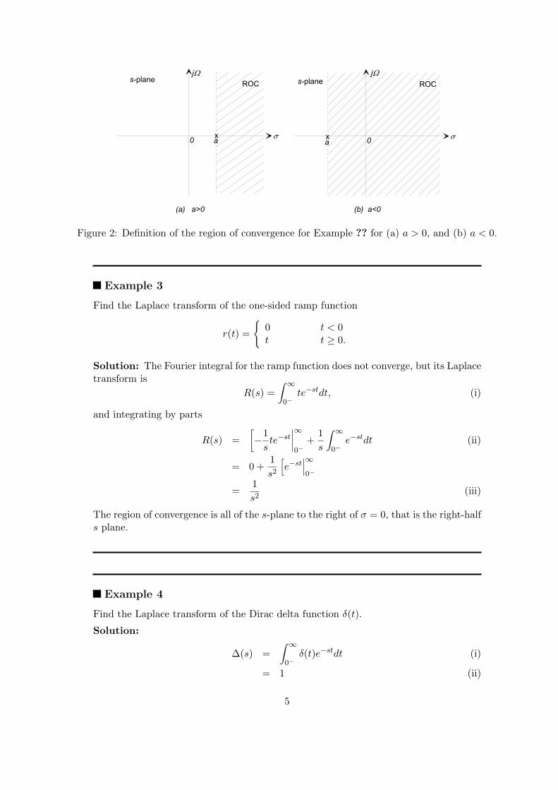
The integral will converge only if σ > a and therefore the region of convergence is the region of the s-plane to the right of σ = a, as shown in Fig. ??. Clearly the imaginary axis lies within the ROC, and the Fourier transform exists, only if a < 0.
4
x s
R O C
a0 x s
R O C
a 0
j W
( a ) a > 0 ( b ) a < 0
s - p l a n e s - p l a n ej W
Figure 2: Definition of the region of convergence for Example ?? for (a) a > 0, and (b) a < 0.
Example 3
Find the Laplace transform of the one-sided ramp function �
0 t < 0 r(t) =
t t ≥ 0.
Solution: The Fourier integral for the ramp function does not converge, but its Laplace transform is
R(s) = � ∞
te−stdt, (i) 0−
and integrating by parts
R(s) =
=
�
− 1 s te−st
����∞
0− +
0 + 1 s2
�e−st
���∞
0−
1 s
� ∞
0− e−stdt (ii)
= 1 s2 (iii)
The region of convergence is all of the s-plane to the right of σ = 0, that is the right-half s plane.
Example 4
Find the Laplace transform of the Dirac delta function δ(t).
Solution:
Δ(s) =
=
� ∞
0− δ(t)e−stdt
1
(i)
(ii)
5
by the sifting property of the impulse function. Thus δ(t) has a similar property in the Fourier and Laplace domains; its transform is unity and it converges everywhere.
Example 5
Find the Laplace transform of a one-sided sinusoidal function �
0 t ≤ 0. x(t) =
sinΩ0t t > 0.
Solution: The Laplace transform is � ∞
X(s) = sin(Ω0t)e−stdt, (i) 0−
and the sine may be expanded as a pair of complex exponentials using the Euler formula
1 � ∞ �
e−(σ+j(Ω−Ω0))t − e−(σ+j(Ω+Ω0))t� dtX(s) =
j2 0−(ii)
� 1
e−(σ+j(Ω−Ω0))t
����∞ �
1 e−(σ+j(Ω+Ω0))t
����∞
= −σ + j(Ω − Ω0)
− −σ + j(Ω + Ω0)0− 0−
Ω0 = (σ + jΩ)2 + Ω2
0
Ω0 = (iii) s2 + Ω2
0
for all σ > 0.
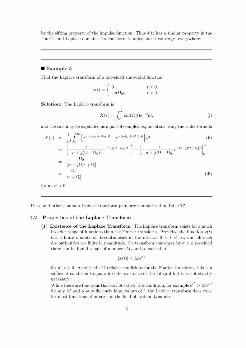
These and other common Laplace transform pairs are summarized in Table ??.
1.2 Properties of the Laplace Transform
(1) Existence of the Laplace Transform The Laplace transform exists for a much broader range of functions than the Fourier transform. Provided the function x(t) has a finite number of discontinuities in the interval 0 < t < ∞, and all such discontinuities are finite in magnitude, the transform converges for σ > α provided there can be found a pair of numbers M , and α, such that
|x(t)| ≤ Meαt
for all t ≥ 0. As with the Dirichelet conditions for the Fourier transform, this is a sufficient condition to guarantee the existence of the integral but it is not strictly necessary. While there are functions that do not satisfy this condition, for example et2
> Meαt
for any M and α at sufficiently large values of t, the Laplace transform does exist for most functions of interest in the field of system dynamics.
6
x(t) for t ≥ 0 X(s)
δ(t) 1
1 us(t)
s 1
t 2s
k!kt k+1s 1
e−at
s + a k!
tk e−at
(s + a)k+1
a1 e−at
s(s + a) ab
−
1 + b
be−at −
a − a
be−bt
a(s + a)(s + b)a −
scosΩt
s2 + Ω2
ΩsinΩt
s2 + Ω2
Ωs e−at (Ω cos Ωt − a sinΩt)
(s + a)2 + Ω2
Table 1: Table of Laplace transforms X(s) of some common causal functions of time x(t).
7
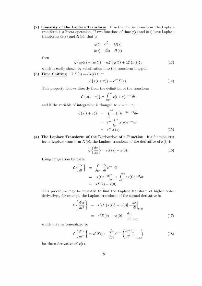
(2) Linearity of the Laplace Transform Like the Fourier transform, the Laplace transform is a linear operation. If two functions of time g(t) and h(t) have Laplace transforms G(s) and H(s), that is
g(t) L G(s)⇐⇒
h(t) L H(s)⇐⇒
then L{ag(t) + bh(t)} = aL{g(t)} + bL{h(t)} . (13)
which is easily shown by substitution into the transform integral. (3) Time Shifting If X(s) = Lx(t) then
L{x(t + τ)} = e sτ X(s). (14)
This property follows directly from the definition of the transform � ∞
x(t + τ)e−stdtL{x(t + τ )} = 0−
and if the variable of integration is changed to ν = t + τ , � ∞
L{x(t + τ)} = 0−
x(ν)e−s(ν−τ )dν
sτ � ∞
= e x(ν)e−sν dν 0−
= e sτ X(s). (15)
(4) The Laplace Transform of the Derivative of a Function If a function x(t) has a Laplace transform X(s), the Laplace transform of the derivative of x(t) is
� dx
�
L dt
= sX(s) − x(0). (16)
Using integration by parts �
dx�
= � ∞ dx
e−stdtL dt 0− dt ���x(t)e−st
���∞
� ∞ sx(t)e−stdt= +
0− 0−
= sX(s) − x(0).
This procedure may be repeated to find the Laplace transform of higher order derivatives, for example the Laplace transform of the second derivative is
� d2x
� dx
����L dt2 = s [sL{x(t)} − x(0)] −
dt t=0
dx����= s 2X(s) − sx(0) − (17)
dt t=0
which may be generalized to
n n 1
L �
d
dt
x�
= s nX(s) − �
s n−i
� d
dt
i−
i−
x�����
�
(18)n 1
i=1 t=0
for the n derivative of x(t).
8
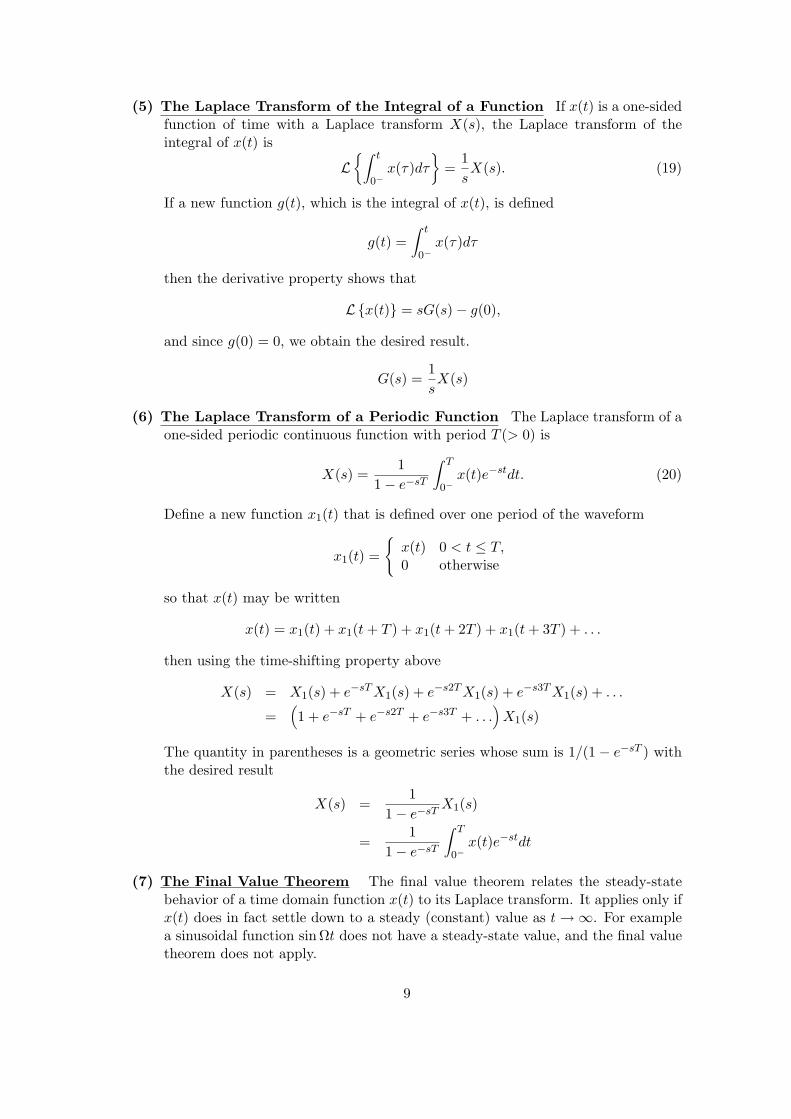
(5) The Laplace Transform of the Integral of a Function If x(t) is a one-sided function of time with a Laplace transform X(s), the Laplace transform of the integral of x(t) is �� t
x(τ)dτ �
=1 X(s). (19)L
0− s
If a new function g(t), which is the integral of x(t), is defined
� t g(t) = x(τ)dτ
0−
then the derivative property shows that
L{x(t)} = sG(s) − g(0),
and since g(0) = 0, we obtain the desired result.
1 G(s) = X(s)
s
(6) The Laplace Transform of a Periodic Function The Laplace transform of a one-sided periodic continuous function with period T (> 0) is
1 � T
X(s) = x(t)e−stdt. (20)1 − e−sT
0−
Define a new function x1(t) that is defined over one period of the waveform �
x(t) 0 < t ≤ T, x1(t) =
0 otherwise
so that x(t) may be written
x(t) = x1(t) + x1(t + T ) + x1(t + 2T ) + x1(t + 3T ) + . . .
then using the time-shifting property above
X(s) = X1(s) + e−sT X1(s) + e−s2T X1(s) + e−s3T X1(s) + . . .
= �1 + e−sT + e−s2T + e−s3T + . . .
� X1(s)
The quantity in parentheses is a geometric series whose sum is 1/(1 − e−sT ) with the desired result
1 X(s) =
1 − e−sT X1(s)
1 � T
x(t)e−stdt= 1 − e−sT
0−
(7) The Final Value Theorem The final value theorem relates the steady-state behavior of a time domain function x(t) to its Laplace transform. It applies only if x(t) does in fact settle down to a steady (constant) value as t →∞. For example a sinusoidal function sin Ωt does not have a steady-state value, and the final value theorem does not apply.
9

If x(t) and its first derivative both have Laplace transforms, and if limt→∞ x(t) exists then
lim x(t) = lim sX(s) (21) t→∞ s→0
To prove the theorem, consider the limit as s approaches zero in the Laplace transform of the derivative
lim � ∞ �
dx(t)
�
e−stdt = lim [sX(s) − x(0)] s 0 dt s 0→ 0− →
from the derivative property above. Since lims 0 e−st = 1 →
� ∞ � d
�
0− dtx(t) dt = x(t) |∞0−
= x(∞) − x(0) = lim sX(s) − x(0),
s 0→
from which we conclude x(∞) = lim sX(s).
s 0→
1.3 Computation of the Inverse Laplace Transform
Evaluation of the inverse Laplace transform integral, defined in Eq. (??), involves contour integration in the region of convergence in the complex plane, along a path parallel to the imaginary axis. In practice this integral is rarely solved, and the inverse transform is found by recourse to tables of transform pairs, such as Table ??. In linear system theory, including signal processing, Laplace transforms frequently appear as rational functions of the complex variable s, that is
N(s)X(s) =
D(s)
where the degree of the numerator polynomial N(s) is at most equal to the degree of the denominator polynomial D(s). The method of partial fractions may be used to express X(s) as a sum of simpler rational functions, all of which have well known inverse transforms, and the inverse transform may be found by simple table lookup. For example, suppose that X(s) may be written in factored form
(s + b1)(s + b2) . . . (s + bm)X(s) = K
(s + a1)(s + a2) . . . (s + an)
where n ≥ m, and a1, a2, . . . , an and b1, b2, . . . , bm are all either real or appear in complex conjugate pairs, if all of the ai are distinct, then the transform may be written as a sum of first-order terms
X(s) = A1 +
A2 + . . . + An
s + a1 s + a2 s + an
where the partial fraction coefficients A1, A2 . . . An are found from the residues
N(s)�
Ai = �(s + ai)
D(s) .
s=−ai
From the table of transforms in Table ?? each first-order term corresponds to an exponential time function,
e−at L 1 ,⇐⇒
s + a
10
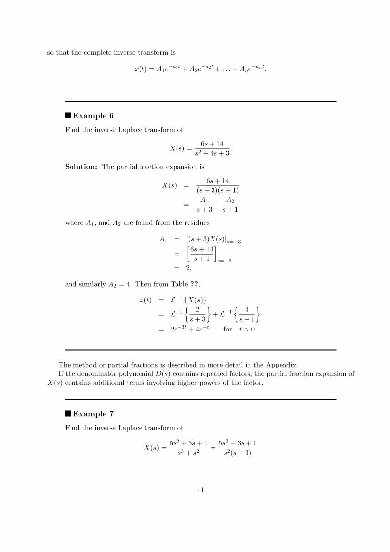
so that the complete inverse transform is
x(t) = A1e−a1t + A2e
−a2t + . . . + Ane−ant .
Example 6
Find the inverse Laplace transform of
6s + 14 X(s) = .
s2 + 4s + 3
Solution: The partial fraction expansion is
6s + 14 X(s) =
(s + 3)(s + 1) A1 A2 = +
s + 3 s + 1
where A1, and A2 are found from the residues
A1 = [(s + 3)X(s)]s=−3 � 6s + 14
�
= s + 1 s=−3
= 2,
and similarly A2 = 4. Then from Table ??,
x(t) = L−1 {X(s)}
= L−1 �
2 �
+ L−1 �
4 �
s + 3 s + 1
= 2e−3t + 4e−t for t > 0.
The method or partial fractions is described in more detail in the Appendix. If the denominator polynomial D(s) contains repeated factors, the partial fraction expansion of
X(s) contains additional terms involving higher powers of the factor.
Example 7
Find the inverse Laplace transform of
5s2 + 3s + 1 5s2 + 3s + 1 X(s) = =
s3 + s2 s2(s + 1)
11

Solution In this case there is a repeated factor s2 in the denominator, and the partial fraction expansion contains an additional term:
X(s) = A1 +
A2 + A3
s s2 s + 1 2 1 3
= + + . (i) s s2 s + 1
The inverse transform of the three components can be found in Table ??, and the total solution is therefore
x(t) = L−1 {X(s)}
= 2L−1 �
1�
+ L−1 �
1 �
+ 3L−1 �
1 �
s s2 s + 1 = 2 + t + 3e−t for t > 0.
2 Laplace Transform Applications in Linear Systems
2.1 Solution of Linear Differential Equations
The use of the derivative property of the Laplace transform generates a direct algebraic solution method for determining the response of a system described by a linear input/output differential equation. Consider an nth order linear system, completely relaxed at time t = 0, and described by
dny dn−1y dy an
dtn + an−1 dtn−1 + . . . + a1
dt + a0y =
dmu dm−1u du bm
dtm + bm−1 dtm−1 + . . . + b1
dt + b0u. (22)
In addition assume that the input function u(t), and all of its derivatives are zero at time t = 0, and that any discontinuities occur at time t = 0+ . Under these conditions the Laplace transforms of the derivatives of both the input and output simplify to
n n
L �
d
dt
y �
= s nY (s), and L �
d
dt
u�
= s nU(s)n n
so that if the Laplace transform of both sides is taken �ans n + an−1s n−1 + . . . + a1s + a0
� Y (s) =
�bms m + bm−1s m−1 + . . . + b1s + b0
� U(s) (23)
which has had the effect of reducing the original differential equation into an algebraic equation in the complex variable s. This equation may be rewritten to define the Laplace transform of the output:
Y (s) = bmsm + bm−1s
m−1 + . . . + b1s + b0 U(s) (24)
ansn + an−1sn−1 + . . . + a1s + a0
= H(s)U(s) (25)
12
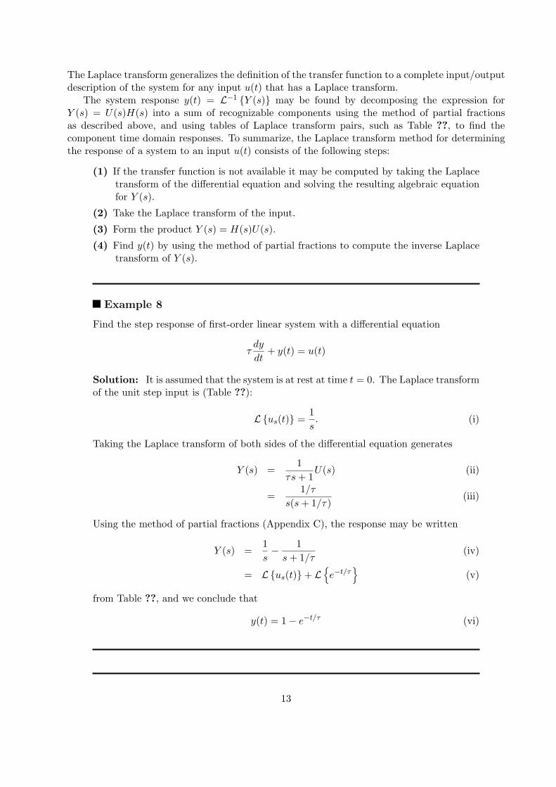
The Laplace transform generalizes the definition of the transfer function to a complete input/output description of the system for any input u(t) that has a Laplace transform.
The system response y(t) = L−1 {Y (s)} may be found by decomposing the expression for Y (s) = U(s)H(s) into a sum of recognizable components using the method of partial fractions as described above, and using tables of Laplace transform pairs, such as Table ??, to find the component time domain responses. To summarize, the Laplace transform method for determining the response of a system to an input u(t) consists of the following steps:
(1) If the transfer function is not available it may be computed by taking the Laplace transform of the differential equation and solving the resulting algebraic equation for Y (s).
(2) Take the Laplace transform of the input.
(3) Form the product Y (s) = H(s)U(s).
(4) Find y(t) by using the method of partial fractions to compute the inverse Laplace transform of Y (s).
Example 8
Find the step response of first-order linear system with a differential equation
τ dy
+ y(t) = u(t)dt
Solution: It is assumed that the system is at rest at time t = 0. The Laplace transform of the unit step input is (Table ??):
1 L{us(t)} = s. (i)
Taking the Laplace transform of both sides of the differential equation generates
1 Y (s) = U(s) (ii)
τs + 1 1/τ
= (iii) s(s + 1/τ)
Using the method of partial fractions (Appendix C), the response may be written
1 1 Y (s) =
s −
s + 1/τ (iv)
= L{us(t)} + L �e−t/τ
� (v)
from Table ??, and we conclude that
y(t) = 1 − e−t/τ (vi)
13
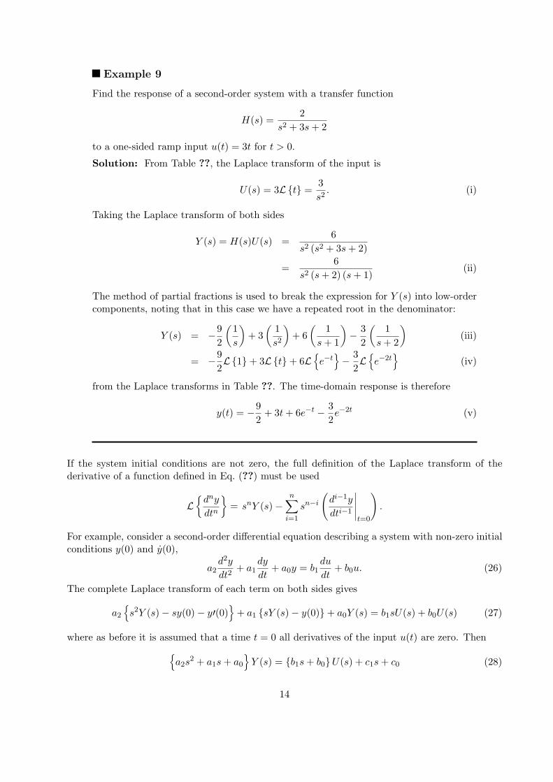
Example 9
Find the response of a second-order system with a transfer function
2 H(s) =
s2 + 3s + 2
to a one-sided ramp input u(t) = 3t for t > 0.
Solution: From Table ??, the Laplace transform of the input is
3 U(s) = 3L{t} = . (i)
s2
Taking the Laplace transform of both sides
6 Y (s) = H(s)U(s) =
s2 (s2 + 3s + 2) 6
= (ii) s2 (s + 2) (s + 1)
The method of partial fractions is used to break the expression for Y (s) into low-order components, noting that in this case we have a repeated root in the denominator:
9 �
1 �
1 �
1 �
3 �
1 �
Y (s) = −2 s
�
+ 3 s
�
+ 6 s + 1
− 2 s + 2
(iii)2
= −29 L{1} + 3L{t} + 6L
�e−t
� −
23 L
�e−2t
� (iv)
from the Laplace transforms in Table ??. The time-domain response is therefore
9 3 y(t) = −
2 + 3t + 6e−t −
2e−2t (v)
If the system initial conditions are not zero, the full definition of the Laplace transform of the derivative of a function defined in Eq. (??) must be used
� dny
� nn−i
� di−1y
�����
�
L dtn = s nY (s) −
� s
dti−1 . i=1 t=0
For example, consider a second-order differential equation describing a system with non-zero initial conditions y(0) and y(0),
d2y dy du a2 + a1 + a0y = b1 + b0u. (26)
dt2 dt dt The complete Laplace transform of each term on both sides gives
a2
�s 2Y (s) − sy(0) − y�(0)
� + a1 {sY (s) − y(0)} + a0Y (s) = b1sU(s) + b0U(s) (27)
where as before it is assumed that a time t = 0 all derivatives of the input u(t) are zero. Then �a2s 2 + a1s + a0
� Y (s) = {b1s + b0} U(s) + c1s + c0 (28)
14

where c1 = a2 (y(0) + y(0)) and c0 = a1y(0). The Laplace transform of the output is the superposition of two terms; one a forced response due to u(t), and the second a function of the initial conditions:
Y (s) = b1s + b0
U(s) + c2s + c0
. (29) a2s2 + a1s + a0 a2s2 + a1s + a0
The time-domain response also has two components
y(t) = L−1 �
b1s + b0 U(s)
�
+ L−1 �
c1s + c0 �
(30) a2s2 + a1s + a0 a2s2 + a1s + a0
each which may be found using the method of partial fractions.
Example 10
A mass m = 18 kg. is suspended on a spring of stiffness K = 162 N/m. At time t = 0 the mass is released from a height y(0) = 0.1 m above its rest position. Find the resulting unforced motion of the mass.
Solution: The system has a homogeneous differential equation
d2y k + y = 0 (i)
dt2 m
and initial conditions y(0) = 0.1 and y(0) = 0. The Laplace transform of the differential equation is �
s 2Y (s) − 0.1s�
+ 9Y (s) = 0 (ii) �s 2 + 9
� Y (s) = 0.1s (iii)
so that
s y(t) = 0.1L−1
� �
(iv) s2 + 9
= 0.1 cos 3t (v)
from Table ??.
2.2 The Convolution Property
The Laplace domain system representation has the same multiplicative input/output relationship as the Fourier transform domain. If a system input function u(t) has both a Fourier transform and a Laplace transform
u(t) F U(jΩ)⇐⇒
u(t) L U(s),⇐⇒
a multiplicative input/output relationship between system input and output exists in both the Fourier and Laplace domains
Y (jΩ) = U(jΩ)H(jΩ) Y (s) = U(s)H(s).
15
Consider the product of two Laplace transforms:
F (s)G(s) = � ∞
f(ν)e−sν dν. � ∞
g(τ)e−sτ dτ −∞ −∞� ∞ � ∞
= f(ν)g(τ )e−s(ν+τ)dτdν, −∞ −∞
and with the substitution t = ν + τ
e−stdtF (s)G(s) = � ∞ �� ∞
f(t − τ)g(τ )dτ
�
−∞ −∞
= � ∞
(f(t) ⊗ g(t)) e−stdt −∞
= L{f(t) ⊗ g(t)} . (31)
The duality between the operations of convolution and multiplication therefore hold for the Laplace domain
f(t) ⊗ g(t) L F (s)G(s). (32)⇐⇒
2.3 The Relationship between the Transfer Function and the Impulse Response
The impulse response h(t) is defined as the system response to a Dirac delta function δ(t). Because the impulse has the property that its Laplace transform is unity, in the Laplace domain the transform of the impulse response is
h(t) = L−1 {H(s)U(s)} = L−1 {H(s)} .
In other words, the system impulse response and the transfer function form a Laplace transform pair
h(t) L H(s) (33)⇐⇒
which is analogous to the Fourier transform relationship between the impulse response and the frequency response.
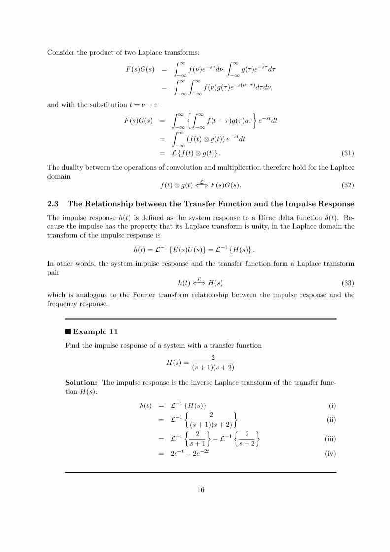
Example 11
Find the impulse response of a system with a transfer function
2 H(s) =
(s + 1)(s + 2)
Solution: The impulse response is the inverse Laplace transform of the transfer function H(s):
h(t) = L−1 {H(s)} (i)
= L−1 �
2 �
(ii)(s + 1)(s + 2)
2 2 = L−1
�
s + 1
�
− L−1 �
s + 2
�
(iii)
= 2e−t − 2e−2t (iv)
16
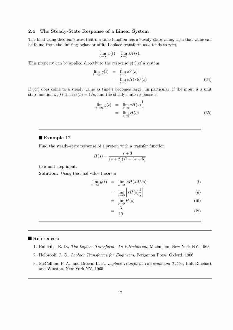
2.4 The Steady-State Response of a Linear System
The final value theorem states that if a time function has a steady-state value, then that value can be found from the limiting behavior of its Laplace transform as s tends to zero,
lim x(t) = lim sX(s). t→∞ s→0
This property can be applied directly to the response y(t) of a system
lim y(t) = lim sY (s) t→∞ s→0
= lim sH(s)U(s) (34) s 0→
if y(t) does come to a steady value as time t becomes large. In particular, if the input is a unit step function us(t) then U(s) = 1/s, and the steady-state response is
1lim y(t) = lim sH(s) t→∞ s→0 s
= lim H(s) (35) s 0→
Example 12
Find the steady-state response of a system with a transfer function
s + 3 H(s) =
(s + 2)(s2 + 3s + 5)
to a unit step input.
Solution: Using the final value theorem
lim y(t) = lim [sH(s)U(s)] (i) t→∞ s→0 �
1�
= lim sH(s) (ii) s 0 s→
= lim H(s) (iii) s 0→3
= (iv)10
References:
1. Rainville, E. D., The Laplace Transform: An Introduction, Macmillan, New York NY, 1963
2. Holbrook, J. G., Laplace Transforms for Engineers, Pergamon Press, Oxford, 1966
3. McCollum, P. A., and Brown, B. F., Laplace Transform Thereoms and Tables, Holt Rinehart and Winston, New York NY, 1965
17

Appendix
Partial Fractions Rational functions of the form
bmsm + bm−1sm−1 + . . . + b1s + b0
F (s) = (36) ansn + an−1sn−1 + . . . + a1s + a0
N(s) =
D(s)
occur frequently in Laplace transform analysis. If the function F (s) is a proper rational function of s, that is it has a numerator polynomial N(s) of degree m, and a denominator polynomial D(s) of degree n with m < n, and with no factors in common, then the method of partial fraction decomposition will allow F (s) to expressed as a sum of simpler rational functions
F (s) = F1(s) + F2(s) + . . . + Fn(s)
where the component functions Fi(s) are of the form
A Bs + C or . (37)
(s + a)k (s2 + bs + c)k
The nature and number of the terms in the partial fraction expansion is determined by the factors of the denominator polynomial D(s).
The linear factors of any polynomial with real coefficients, such as D(s), are either real or appear in complex conjugate pairs. Each pair of complex conjugate factors may be considered to represent two distinct complex factors, or they may be combined to generate a quadratic factor with real coefficients. For example the polynomial
D(s) = s 3 − s 2 − s − 15
may be written in terms of one real linear and one real quadratic factor, or a real linear factor and a pair of complex linear factors
D(s) = (s − 3)(s 2 + 2s + 5)
= (s − 3)(s + (1 + 2j))(s + (1 − 2j))
Each representation will produce a different, but equivalent, set of partial fractions. The choice of the representation will be dependent upon the particular application. The use of the quadratic form will however avoid the necessity for complex arithmetic in the expansion.
Assume that F (s) is written so that D(s) has a leading coefficient of unity, and that D(s) has been factored completely into its linear and quadratic factors. Then let all repeated factors be collected together so that D(s) may be written as a product of distinct factors of the form
(s + ai)pi or (s 2 + bis + ci)
pi
where pi is the multiplicity of the factor, and where the coefficients ai in the linear factors may be either real or complex, but the coefficients bi and ci in any quadratic factors must be real. Once this is done the partial fraction representation of F (s) is composed of the following terms
18

Linear Factors: For each factor of D(s) of the form (s + ai)p, there will be a set of p terms
Ai1 Ai2 Aip+ + . . . +
s + ai (s + ai)2 (s + ai)p
where Ai1, Ai2, . . . , Aip are constants to be determined.
Quadratic Factors: In general for each factor of D(s) of the form (s2 + bis + ci)p, there
will be a set of p terms
Bi1s + Ci1 Bi2s + Ci2 Bips + Cip+ + . . . +
s2 + bis + ci (s2 + bis + ci)2 (s2 + bis + ci)k
where Bi1, Bi2, . . . , Bip and Ci1, Ci2, . . . , Cip are constants to be determined.
Example 13
Determine the form of a partial fraction expansion for the rational function
2 F (s) = .
s2 + 3s + 2
where N(s) = 2 and D(s) = s2 + 3s + 2. If the denominator is factored the function may be written
2 2 F (s) = =
s2 + 3s + 2 (s + 1)(s + 2) and according to the rules above each of the two linear factors will introduce a single term into the partial fraction expansion
F (s) = A1 +
A2
s + 1 s + 2
where A1 and A2 have to be found.
Example 14
Determine the form of the terms in a partial fraction expansion for the rational function
2s + 3 F (s) = .
s2(s + 1)(s2 + 2s + 5)
This example has a repeated factor s2, a single real factor (s+1), and a quadratic factor (s2 + 2s + 5) = (s + (1 + 2j))(s + (1 − 2j)). The partial fraction expansion may be written in two possible forms; with the quadratic term
F (s) = A11 +
A12 + A2 +
B3s + C3
s s2 s + 1 s2 + 2s + 5
or in terms of a pair of complex factors
A11 A12 A3 A4 A5F (s) =
s +
s2 + s + 1
+ s + (1 + 2j)
+ s + (1 − 2j)
19
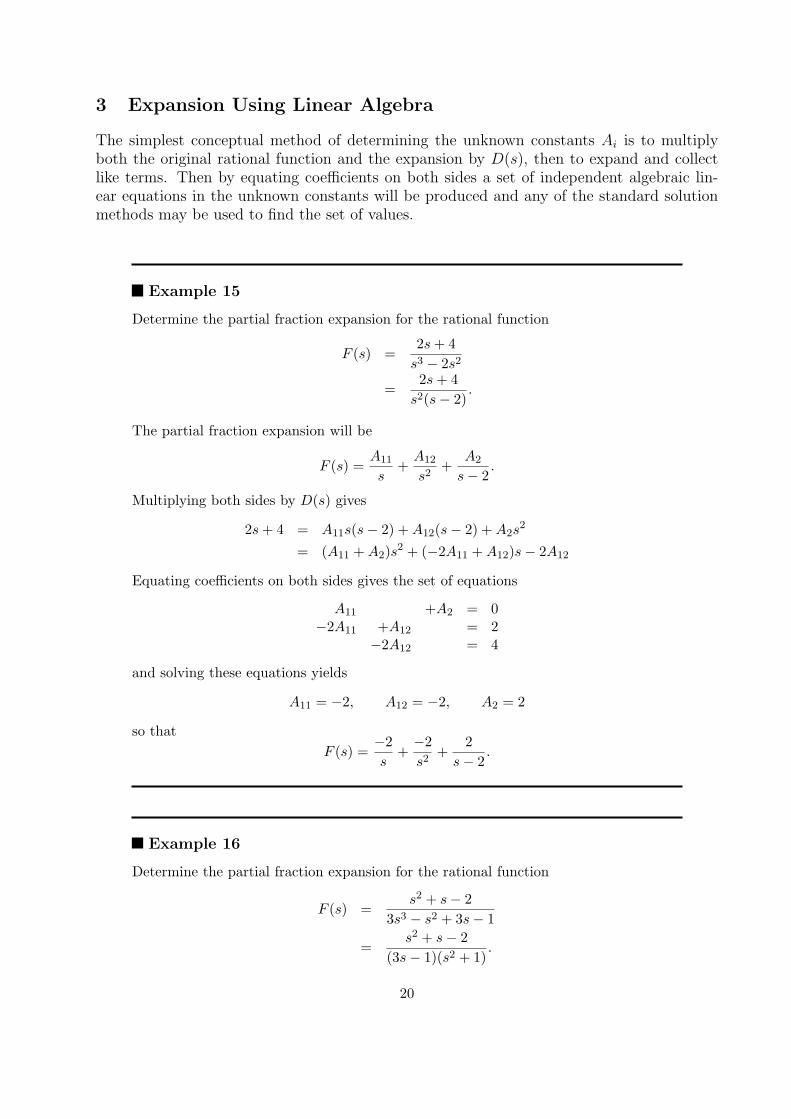
3 Expansion Using Linear Algebra
The simplest conceptual method of determining the unknown constants Ai is to multiply both the original rational function and the expansion by D(s), then to expand and collect like terms. Then by equating coefficients on both sides a set of independent algebraic linear equations in the unknown constants will be produced and any of the standard solution methods may be used to find the set of values.
Example 15
Determine the partial fraction expansion for the rational function
2s + 4 F (s) =
3 2s − 2s 2s + 4
= . s2(s − 2)
The partial fraction expansion will be
F (s) = A11 +
A12 + A2
. s s2 s − 2
Multiplying both sides by D(s) gives
2s + 4 = A11s(s − 2) + A12(s − 2) + A2s 2
= (A11 + A2)s 2 + (−2A11 + A12)s − 2A12
Equating coefficients on both sides gives the set of equations
A11 +A2 = 0 −2A11 +A12 = 2
−2A12 = 4
and solving these equations yields
A11 = −2, A12 = −2, A2 = 2
so that F (s) =
−s 2
+ −s2
2+
s − 2
2.
Example 16
Determine the partial fraction expansion for the rational function
F (s) = s2 + s − 2
3s3 − s2 + 3s − 1 s2 + s − 2
= .(3s − 1)(s2 + 1)
20
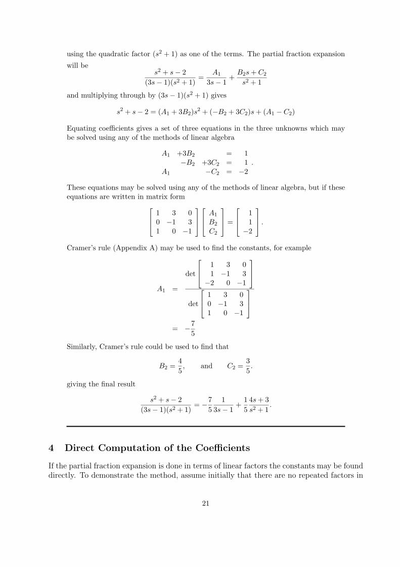
using the quadratic factor (s2 + 1) as one of the terms. The partial fraction expansion
will be s2 + s − 2 A1 B2s + C2 = +
(3s − 1)(s2 + 1) 3s − 1 s2 + 1
and multiplying through by (3s − 1)(s2 + 1) gives
s 2 + s − 2 = (A1 + 3B2)s 2 + (−B2 + 3C2)s + (A1 − C2)
Equating coefficients gives a set of three equations in the three unknowns which may be solved using any of the methods of linear algebra
⎤⎥
A1 +3B2 = 1 −B2 +3C2 = 1 .
A1 −C2 = −2
⎤⎥
These equations may be solved using any of the methods of linear algebra, but if these equations are written in matrix form
⎦ = ⎦ .
⎡
⎢⎣
⎡
⎢⎣
⎤
⎥⎦
⎡
⎢⎣
1 3 0 1A1
0 −1 3 0
1B2
1
⎡
⎢⎣
−1
det
−2C2
Cramer’s rule (Appendix A) may be used to find the constants, for example ⎤
⎥⎦
1 3 01 −1 3
−2 0 −1A1 = ⎡
⎢⎣det
7 = −
5
Similarly, Cramer’s rule could be used to find that
⎤
⎥⎦
1 3 00 −1 3 1 0 −1
4 3 B2 = , and C2 = .
5 5
giving the final result
s2 + s − 2 7 1 1 4s + 3 (3s − 1)(s2 + 1)
= −5 3s − 1
+5 s2 + 1
.
Direct Computation of the Coefficients
If the partial fraction expansion is done in terms of linear factors the constants may be found directly. To demonstrate the method, assume initially that there are no repeated factors in
21
4
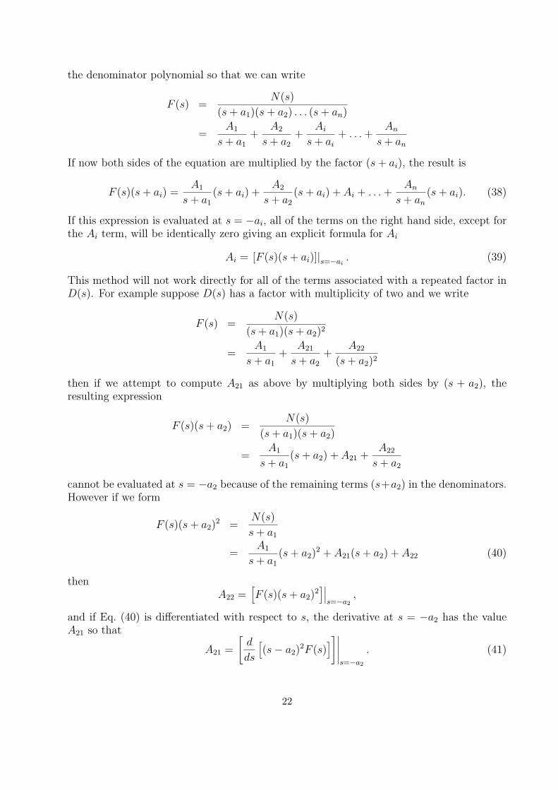
the denominator polynomial so that we can write
N(s)F (s) =
(s + a1)(s + a2) . . . (s + an) A1 A2 Ai An
= + + + . . . + s + a1 s + a2 s + ai s + an
If now both sides of the equation are multiplied by the factor (s + ai), the result is
A1 A2 AnF (s)(s + ai) = (s + ai) + (s + ai) + Ai + . . . + (s + ai). (38)
s + a1 s + a2 s + an
If this expression is evaluated at s = −ai, all of the terms on the right hand side, except for the Ai term, will be identically zero giving an explicit formula for Ai
Ai = [F (s)(s + ai)]|s=−ai . (39)
This method will not work directly for all of the terms associated with a repeated factor in D(s). For example suppose D(s) has a factor with multiplicity of two and we write
N(s)F (s) =
(s + a1)(s + a2)2
A1 A21 A22 = + +
s + a1 s + a2 (s + a2)2
then if we attempt to compute A21 as above by multiplying both sides by (s + a2), the resulting expression
N(s)F (s)(s + a2) =
(s + a1)(s + a2) A1 A22
= (s + a2) + A21 + s + a1 s + a2
cannot be evaluated at s = −a2 because of the remaining terms (s+a2) in the denominators. However if we form
F (s)(s + a2)2 =
N(s) s + a1
= A1
(s + a2)2 + A21(s + a2) + A22 (40)
s + a1
then A22 =
�F (s)(s + a2)
2���� ,
s=−a2
and if Eq. (40) is differentiated with respect to s, the derivative at s = −a2 has the value A21 so that �
d A21 =
�(s − a2)
2F (s)������� . (41)
ds s=−a2
22
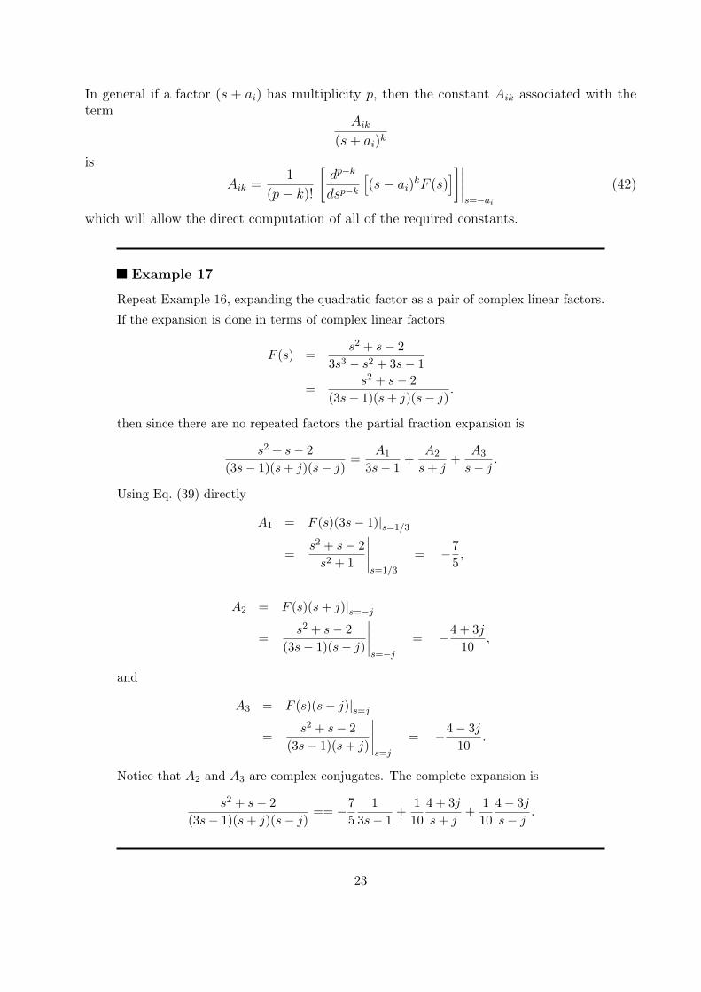
In general if a factor (s + ai) has multiplicity p, then the constant Aik associated with the term
Aik
(s + ai)k
is
Aik = 1
(p − k)!
� dp−k
dsp−k
�(s − ai)
kF (s)�������
s=−ai
(42)
which will allow the direct computation of all of the required constants.
Example 17
Repeat Example 16, expanding the quadratic factor as a pair of complex linear factors.
If the expansion is done in terms of complex linear factors
s2 + s − 2 F (s) =
3s3 − s2 + 3s − 1 s2 + s − 2
= .(3s − 1)(s + j)(s − j)
then since there are no repeated factors the partial fraction expansion is
s2 + s − 2 A1 A2 A3 = + + .(3s − 1)(s + j)(s − j) 3s − 1 s + j s − j
Using Eq. (39) directly
A1 = F (s)(3s − 1) s=1/3
s2 + s − 2�����
| 7
= = , s2 + 1
−5
s=1/3
A2 = F (s)(s + j) s=−j
s2 + s −| 2
�����4 + 3j
= (3s − 1)(s − j)
s=−j
= − 10
,
and
A3 = F (s)(s − j)|s=j
s2 + s − 2 �����
4 − 3j= = .
(3s − 1)(s + j) −
10 s=j
Notice that A2 and A3 are complex conjugates. The complete expansion is
s2 + s − 2 == −
7 1 +
1 4 + 3j +
1 4 − 3j.
(3s − 1)(s + j)(s − j) 5 3s − 1 10 s + j 10 s − j
23
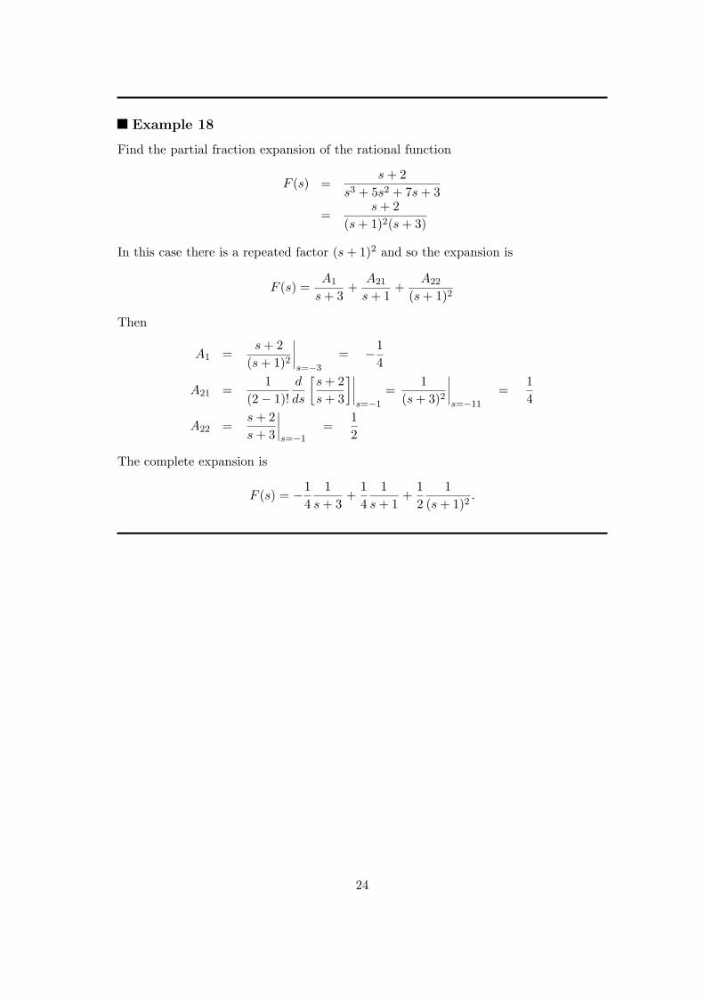
Example 18
Find the partial fraction expansion of the rational function
s + 2 F (s) =
s3 + 5s2 + 7s + 3 s + 2
= (s + 1)2(s + 3)
In this case there is a repeated factor (s + 1)2 and so the expansion is
F (s) = A1 +
A21 + A22
s + 3 s + 1 (s + 1)2
Then
s + 2 ����
1 A1 = =
(s + 1)2 s=−3
−4
1 d � s + 2
�����1
����1
A21 = = = (2 − 1)! ds s + 3 s=−1 (s + 3)2
s=−11 4
s + 2��� 1
A22 = = s + 3 �
s=−1 2
The complete expansion is
1 1 1 1 1 1 F (s) = −
4 s + 3 +
4 s + 1 +
2 (s + 1)2 .
24