22-1 Copyright 2010 McGraw-Hill Australia Pty Ltd PowerPoint slides to accompany Croucher, Introductory Mathematics and Statistics, 5e Chapter 22 Analysis

22-1Copyright 2010 McGraw-Hill Australia Pty Ltd PowerPoint slides to accompany Croucher, Introductory Mathematics and Statistics, 5e

Chapter 22

Analysis of Frequency Data

Introductory Mathematics & Statistics


Learning Objectives

• Understand the meaning of a categorical variable

• Understand the difference between a single-variable problem and a two-variable problem

• Construct a table for a single-variable problem

• Construct a contingency table for a two-variable problem

• Analyse single-variable data

• Analyse two-variable data


22.1 Categorical data

• Data are often non-numerical, in the sense that each individual observation is a description rather than a number

• Averages cannot be used in these circumstances

• Systems where the observations are descriptive (rather than numerical) are described as categorical, because the individuals are being classified into categories

• Examples– What gender are you?– What colour are your eyes?– Do you have a valid driver’s licence?– What suburb do you live in?– Have you ever travelled overseas?– Who is your favourite lecturer?– Do you have an internet connection at home?


22.1 Categorical data (cont…)

• The following statistical questions also involve categorical variables:– Are people who are avid followers of sport more likely to own

a large-screen television than those who do not follow sport?– Does area of residence affect the likelihood of owning a

motor vehicle?– Do people who live in particular part of a city have any

different radio preferences from those who live elsewhere?– Do males and females differ in their level of interests in

attending the opera? – Is there a significantly higher proportion of older wine-

drinkers than younger wine-drinkers?


22.1 Categorical data (cont…)

• These questions may also conveniently be expressed as questions about differences between proportions, such as:– Does the proportion of individuals owning a large-screen

television differ between avid followers of sport and others?– Does the proportion of people who own motor vehicles differ

from one area of residence to another?– Does the proportion of people preferring various radio

stations differ depending on where people live in a city?– Does the proportion of males interested in attending the

opera differ from the proportion for females?– Does the proportion of wine-drinkers differ with age?


22.2 Single-variable categorical data

• It is common practice to have a standard form of presentation

• It is convenient to work with frequency data, that is data in which the number of occurrences of each category is recorded

• A frequency table is a table in which the number of occurrences of each category is recorded

Table 22.1 Outcomes of 60 rolls of a fair six-sided die

Category 1 2 3 4 5 6 Total

Frequency 8 7 12 13 5 15 60


22.3 Contingency tables

• Some problems involve two categorical variables, and questions often arise about their relationship

• A two-dimensional table is where one variable is presented along the rows and the other variable down the columns

Table 22.3 A typical contingency table for the residence and internet survey

Internet North South East West Total

Yes 52 47 105 34 238

No 28 63 35 36 162

Total 80 110 140 70 400

Live


22.3 Contingency tables (cont…)

• Contingency tables have characteristics that are common to all such tables. These include:– The final column is a total column– The final row is a total row– It generally does not matter which variable is along the

columns and which is along the rows– Frequencies must add up along each row– Frequencies must add up down each column– The value in the bottom right-hand corner of the table

represents the total number of observations overall. It is often referred to as the grand total frequency


22.4 Analysis of single-variable problems

• The question to be answered is whether an observed set of categorical data is reasonably consistent with what was expected by some prior line of reasoning

• Analysis of single variable problems. The steps involved are known as a goodness-of-fit test

• The steps involved in the analysis of a single variable problem are as follows:1. Construct the null hypothesis for the problem. This usually takes

the general form of: H0: There is no difference between the observed frequencies and the

expected frequencies This should be modified for each individual problem

H1: The alternative hypothesis (using a two-sided alternative)


22.4 Analysis of single-variable problems (cont…)2. Obtain the observed frequencies from the data of the problem

3. Determine the expected frequencies; these are ones we might ‘expect’ to occur if H0 were true

4. Calculate the measure of the discrepancy between the observed and expected frequencies using by the chi-square test statistic

– The symbol 2 is called ‘chi-square’, with the ‘chi’ being pronounced as ‘ky’

– Also, since the square of a number can never be negative, the value of a 2-test statistic can also never be negative

categories all frequency expected

frequencyexpectedfrequencyobserved 22


22.4 Analysis of single-variable problems (cont…)

5. Associated with the test statistic are degrees of freedom. Determine the degrees of freedom for a goodness-of-fit test using:

Degrees of freedom = number of categories – 1

6. Obtain the critical value, from Table 9. Two pieces of information are required: the degrees of freedom (down the left-hand column) and the significance level desired (across the top row)



7. Compare the value of χ2 that you calculated with the critical value from Table 9

If χ2 < the critical value, we cannot reject Ho

If χ2 > the critical value, we reject Ho

8. Based on the outcome of Step 7, draw an appropriate conclusion



ExampleSuppose that a statistician is presented with six-sided die and asked to determine whether it is ‘fair’, that is whether it is equally likely that the outcome will be a 1, 2, 3, 4, 5 or 6 when the die is tossed. The die is rolled a total of 300 times. The outcomes are shown in the following table

Outcome Frequency

1 48

2 57

3 60

4 42

5 44

6 49

Total 300


22.4 Analysis of single-variable problems (cont…)Solution

If the die is really fair, there is a 1/6 probability that any given face will appear at any roll. Thus, in a loose sense, the 300 rolls would be ‘expected’ to yield 300 × 1/6 = 50 occurrences of each face

Step 1: H0: The die is fair

H1: The die is not fair

Step 2: The observed frequencies are the actual values obtained for each category; that is 48, 57, 60, 42, 44 and 49

Step 3: Since H0 assumes that the die is fair, the expected frequency for each category is the same, that is,

300 × 1/6 = 50



Step 4: For the die, the calculations required for the 2-test statistic are:

Step 5: For the die, since there are 6 categories, the degrees of freedom are 6 – 1 = 5

08.5

02.072.028.100.298.008.050

5049

50

5044

50

5042

50

5060

50

5057

50

5048

222

2222



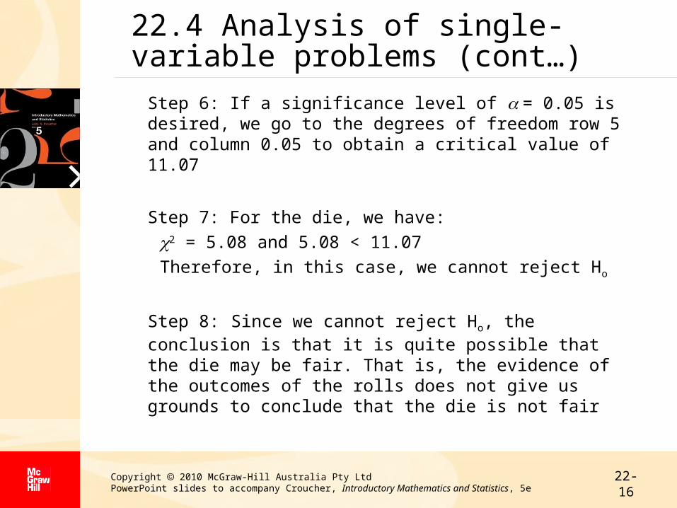
Step 6: If a significance level of = 0.05 is desired, we go to the degrees of freedom row 5 and column 0.05 to obtain a critical value of 11.07

Step 7: For the die, we have:

2 = 5.08 and 5.08 < 11.07

Therefore, in this case, we cannot reject Ho

Step 8: Since we cannot reject Ho, the conclusion is that it is quite possible that the die may be fair. That is, the evidence of the outcomes of the rolls does not give us grounds to conclude that the die is not fair


22.5 Analysis of contingency tables

• The 2 technique can be generalised to the case where two variables are involved

• The data will be in the form of a contingency table with any number of rows and columns

• The steps involved in the analysis of contingency tables are as follows:1. Construct the null hypothesis for the problem. This usually takes the general form that the two variables are independent or that there is no relationship between them

H0: The two variables are independentorH0: There is no relationship between the two variables

The alternative hypothesis (using a two-sided alternative) would be:

H1: The two variables are not independentorH1: There is a relationship between the two variables


22.5 Analysis of contingency tables (cont…)

2. Identify the observed frequencies from the data of the problem. There will be one observed frequency for each cell of the contingency table3. Calculate the expected frequencies, those that we might ‘expect’ to occur if H0 were true. For each cell of the contingency table there will also be an expected frequency. The expected frequency for each cell can be found using:

• The grand total frequency can be found in the bottom right-hand corner of the table

frequencytotalgrand

rowthatforfrequencytotalcolumnthatforfrequencytotal

cellaforfrequencyExpected



4. Calculate the measure of the discrepancy between the observed and expected frequencies using the 2 test statistic. The formula is:

Note that there is one term required in the calculation for each cell of the table.

5. Determine the degrees of freedom for the contingency table

Degrees of freedom =

(number of rows – 1) × (number of columns – 1)

cellsall frequency expected

frequencyexpected frequencyobserved 22



6. Obtain the critical value from Table 9, using both the degrees of freedom and the desired significance level

7. Compare the value of 2 that you calculated with the critical value from Table 9

If 2 < the critical value, we cannot reject H0

If 2 > the critical value, we can reject H0

8. Based on the outcome of Step 7, draw an appropriate conclusion


Summary

• We have understood– the meaning of a categorical variable– the difference between a single-variable problem and a two-

variable problem

• We constructed– a table for a single-variable problem– a contingency table for a two-variable problem

• We analysed single-variable data

• Lastly we analysed two-variable data

Documents

22-1 Copyright 2010 McGraw-Hill Australia Pty Ltd PowerPoint slides to accompany Croucher, Introductory Mathematics and Statistics, 5e Chapter 22 Analysis