Embed Size (px)
Citation preview

ADl-A093 67W VIRGINIA POL.YTECHNIC INST AND STATE UNIV BLACKSBURG -ETC F/S 12/1TUTORIAL ON NARKOV RENEWAL THEORY SENI-RESENERATIVE PROCESSES--ETCWUl
DEC 00 R L DISNEY N0OOIW.77.C-0743UNCLASSIFIED VTRO-0722 fllllllllll
I
I-EEEEEEEEmh.
IIIIIIIIIIIII

11111 11111I1111IL25 NW1.4 111111.6
MICROCOPY RESOLUTION TEST CHART

-4k
'IA'r~

A Tutorial on
Markov Renewal Theory
Semi-Regenerative Processes
and Their Applications
C'
Ralph L. Disney
Gordon Professor
Department of Industrial Engineering and Operations Research
Virginia Polytechnic Institute and State UniversityBlacksburg, Virginia 24061
July, 1980VTR 8007
ISTVJUUTION STA~ttAppo'ed for pr UTc r"',
These notes were prepared for a tutorial session at the fall joint O.R.S.A/T.I.M.S.
Conference held in Colorado Springs, 1980. They were partly supported under the
Office of Naval Research Contract N00014--77-C-0743 (NR042-296) and National
Science Foundation Grant ENG77-22757. Distribution of this document is unlimited.
Reproduction in whole or in part is permitted for any purpose of the United StatesGove rnmen t.

SECURITY CLASSIFICATION OF THIS PAGE (ml., ot& Enteredl
REPORT DOCUMENTATION PAGE BEFORE__COMPLETING__FORM1. REPORT NUMBER (j/ 12 OTACESO O 3. RECIPIENT'S CATALOG NUMBER
Technical Repo'R-817 5- 3 ?94. TITLE (and Subtitle) -- -
Technical I(epewtA Tutorial on Markov Renewal Theory Semi-
-. CONTRACT OR GRANT NUMUER(.)
Dr.R h .i.e N60014-77-C-0743
Department of Industrial Engr. & Operations Res. AEIOKNTU R
Virginia Polytechnic Inst. & 'State University NR042-296Blacksburg, Virginia 24061
11. CON4TROLLING OFFICE NAME AND ADDRESS _z IFRUI
Direc to r, Statistics and Probability Program /( Decw 80Mathematical & Information Sciences Division aEI"WPU800 N. Quincy St., Arlington, VA 22217 107
14. MONITORING AGENCY NAME 6 AOORESS(II different from, Controlli Office) I5. SECURITY CLASS. (of this report)
Unclassifiede'4' I t
[Iro7 DCCL ASSIFICATION/ DOWNGRADING[ aSCHEDUL E
16. DISTRIBUTION STATEMENT (of this Report)
APPROVED FOR PUBLIC RELEASE: DISTRIBUTION UNLIMITED.
17. DISTRIUTION STATEMENT (of the sbeir*Cf entered In Block 20, It different from Report)
III. SUPPLEMENTARY NOTES
19. KEY WORDS (Continue on re.'eree side it necewey mid identify by black ns..ber)
Tutorial, Markov Renewal Processes, Semi-Regenerative Processes,
Applications toCombat Visibility, Queueing Theory, Power Generator Reliability,Medical Emergency, Road Traffic, and Fatigue.
20. A'?51 RACT (Continue on revere side If neceseer and Identify by block numbr).This is a tutorial paper onMarkov renewal processes, semi-regenerative processes and their applicationsto many fields of interest. It was presented inithe tutorial sessions of theO.R.S.A./T.I.M.S. meetings in Colorado Springs, November, 1980.
The paper reviews the basic ingredients of the processes discussed suchas: structure of the process, semi-Markov kernels, Markov renewal functions,and integral equations of semi-regeiterative processes. Considerable time isspent discussing several applications to combat line-of-sight, queueing,
DD ',N", 1473 EDITION Of' I NOV SS IS OBSOLETE
S N 0 102- LF- 0 1.-1- 6601 SECURITY CLASSIFICATION OF THIS PACE (When D41te Entered'

a
police medical emergency systems, disease modelling, power generatorreliability and worker fatigue.
The bibliography of 21 items provides further readings for thebeginner to pursue these topics.
I.J
3,
k . .. .. , .-... ~l,

This report is an interim report of on-going research. It may beamended, corrected or withdrawn, if called for, at the discretion ofthe author.
T,,cession FOr
ie El
41 tia.
2t
23e
Tohr
* .. f.. zv'" -:n<q/or
I": 2; i'.I

Table of Contents
1. Introduction
1.0. Overview ............. .......................... 1i.i. A Simple Problem ........... ...................... 11.2. Observations ............ ........................ 3
II. Markov Renewal Processes
2.0. Introduction ......... ........................ . .. 62.1. A Markov Renewal Process ......... .................. 82.2. An Interpretation ........... ...................... 92.3. Two Applications ........... ...................... 102.4. Some Properties of Qi (t) and the Markov
Renewal Process . ........ .. .................... 132.5. Other Processes as Markov Renewal Processes .. ......... ... 15
2.5.1. Renewal Processes ...... ................ ... 152.5.2. Markov Processes ...... ................. ... 162.5.3. Markov Chains ....... .................. ... 17
2.6. The Markov Renewal Function ...... ................. ... 172.7. The Markov Renewal Equation ...... ................. ... 22
2.8. Summary ............. ........................... 24
III. Semi-Regenerative Processes
3.0. Introduction .......... ........................ ... 243.1. Semi-Regenerative Processes ...... ................. ... 253.2. Some Examples of Semi-Regenerative Processes . ........ ... 28
3.2.1. Forward Recurrence Times .... ............. ... 283.2.2. The Birth Process ........ ................ 313.2.3. The Time Dependent Queue Length
in the M/G/i Queue ....... ................. 323.2.4. A Disease Model ........... ........... . 33
3.2.5. The Minimal Semi-Markov Process .. ......... ... 343.3. Some Properties of Semi-Regenerative Processes . ....... . 343.4. Summary ............. ........................... 36
IV. Examples and Applications
4.0. Introduction .......... ........................ ... 374.1. Examples and Applications ...... .................. ... 39
4.1.1. Visibility ....... .................... ... 404.1.2. Departures from the M/G/l/N Queue . ........ ... 494.1.3. The Time Dependent M/G/1/N Queue .. ......... ... 574.1.4. A Disease Model ........ ................. 614.1.5. Police Emergency Calls ..... .............. ... 694.1.6. The DiMarco Study ...... ................ ... 834.1.7. Other Applications ...... ................ ... 88
4.1.7.1. The Daganzo Study ... .......... ... 884.1.7.2. The Lee Study .... ............ ... 89
4.2. Other Studies ......... ........................ ... 90

V. Summary and Afterword
5.0. Summary .. .............. ............. 91
5.1. Afterword .. .............. ............ 92
VI. Bibliography .. ............... .............. 94

Preface
Modelling stochastic systems is an art. As such one learns by doing.
But the process of learning is long and has a number of steps preliminary to
doing. One must learn some basic concepts of stochastic processes and their
properties. Unfortunately, this step and its output have come to be called
"theoretical" and seem to be viewed with a jaundiced eye as though they were
unnecessary, irrelevant and an impediment to doing.
Except for the gifted few this process of learning must next include
some familiarity with how others have used the theory to study important
problems. This step I would call the study of models. It is not an end,
nor a beginning, but an intermediate step to learning how to do. Unfortu-
nately, most textbooks and many journal pages leave one with the impression
that models previously developed somehow have an intrinsic value and if one
knows enough models then applying the "theory" is just a plug-in exercise.
This may be true in some fields but in operations research we know so little
of the basic "science" of our processes that except in rather rare cases we
do not have coherent models. All applications must cut, paste, extend,
compress, rearrange or even develop models to make them do. The study of
existing models is necessary but not sufficient to the doing of modelling.
It is necessary to see how others have handled the problems of messy data
(Unlike laboratory sciences, operations researchers almost always deal with
messy data.), complexity of systems, systems that just do not satisfy
assumptions of existing models and the like. But this process is not
sufficient to doing modelling by oneself. My non-linearity is not your non-
linearity. My dependence is not your dependence. Therefore, the final

step in learning how to model is to model.
Modelling, it seems to me, cannot be taught in the usual sense that we
use that word. It is clear that it can be learned because many people have
learned how to do it.
These notes try to reach the second of the three levels of modelling.
That is, they try to expose very briefly, models of processes that others
have developed. To understand how these models have been developed will
require considerably more digging than we provide. Some of the studies we
will mention occupy hundreds of pages of discussion. They cannot be
summarized into a "how to do it manual" especially in our relatively few
pages. But when all is said and done these examples are models. They are
not "reality". They are not prescriptions or descriptions of "how to do it".
We start these notes with what we hope is a mildly surprising result
obtained from a simulation of a very simple system. Unravelling the seem-
ing mystery of the example takes us two rather long sections (II and III) to
develop some structure for the random process underlying the example. It will
turn out that the structure developed for that purpose (which has been in the
research literature for about 25 years) has many other uses. In section IV
some of these other uses are exposed. In particular we note, in very brief
summary form, some of the uses to which the results of section II and III
have been put. Here, we continually implore the reader to consult the source
documents. Our discussion is, intended simply to goad the reader into that
literature. In no sense do we do the literature the service it deserves.
Such is not our intention nor could it be done within the confines of space,
time and our short span of interest in rehashing work that others have exposed

well. In section V we summarize where we have been and try to put the
state-of-the-art in perspective in three pages. The bibliography is not
complete in any dimension but a careful reading of the documents therein
will take the reader more deeply into both theory and other applications.
During my years of teaching, I have had the priviledge of working
with some very bright young men and women. To them is due credit for
nearly everything in these notes. The errors are mine and I hope they
will forgive me the distortions I made to their work as I tried to condense
hundreds of pages to these few. Drs. Peter Cherry, Erhan ginlar, Arthur
Cole, Carlos Daganzo, Gilles D'Avignon, Atillio DiMarco, William Hall,
Ralph King, Myun Lee, Gordon Swartzman, Burton Simon, James Solberg, and
Thomas Vlach will recognize how deeply I am indebted to their work in
these pages. Mr. Ziv Barlach did the simulation analysis noted therein and
produced some of the analytic results with which we compared these results
with the simulation. Dr. Robert D. Foley a former student and now valued
colleague read this manuscript as did Dr. Jeffrey Hunter whose good nature
was taken advantage of during his sabbatical leave from the University of
Auckland, New Zealand at VPI & SU. Dr. Hunter was kind enough to share with
me the thesis by Ms. Sim. Finally, what can I say about my right arm, Ms.
Paula Myers? She typed, retyped and re-retyped these pages, always outwardly
good humoredly and met impossible deadlines caused by my normal
procrastination.
Ralph L. Disney
Blacksburg, Virginia
July, 1980

I. INTRODUCTION
1.0. Overview. Our purpose in these notes is to expose some concepts in
stochastic modelling.
Since computer simulation is a widely used tool, we attempt to motivate
our discussion with a problem that was simulated. The problem is very simple,
well known to all operations researchers, has an analytic solution and is easy
to simulate. However, we will see a result that at first glance can be perplex-
ing. In particular a variance estimate made using the computer's output does
not seem to be behaving "as it should". One can guess many reasons for the
anomaly. The sample is not big enough. The simulation was not generating
steady state results. These guys do not know how to simulate. While all of
this may be true, the problem is much deeper than this. To understand and
correct for it takes us far afield. By the time we return to the example
(section 4.1.2) we have discussed a large body of knowledge (sections II and
III). Since that knowledge is considerably more useful than our simplistic
simulation problem, we expose several examples and a few real-life applica-
tions of it.
1.1. A Simple Problem. Let us begin with a very simple problem whose structure
is well known to everyone in operations research. Consider the M/M/l/N queue.
Suppose that we would like to determine, experimentally, the mean time between
departures from such a queue. Such an endeavor is not too far fetched because
in a queueing system this departure process might be the input to other queues
that we wish to study or it might be the output of the system that we wish to
control.

In many experimental studies one seeks not simply a point estimate of such
a thing as a mean but rather one wants an interval estimate, perhaps a confidence
interval. Therefore, let us require of our experimental procedure that we find
the variance of the time between deparLures from the M/M/l/N queue. To make the
matter more precise, let us choose N = 3 and several values for the usual traffic
intensity p = A/p.
Now we know that we probably should choose a large sample to gain precision
in our estimates. Therefore, let us arbitrarily select 100 departure intervals
(not because of any magic formula but simply because I did not have more money
for computing).
One of my students, much more knowledged in simulation than I, simulated
100 steady state departure intervals from a M/M/l/3 queue. We then computed,
using the standard tools of statistics, the mean and standard deviation for
this sample.
A simple piece of stochastic modelling can give us the "true" mean for this
data. The analysis might go as follows.
Consider the queue just after a departure has occurred. At that instant,
the queue left behind is either 0 - the queue is empty or it is not 0 - there
is at least someone in service.
Now if the queue is empty at a departure point (with probability n0 (n))
we must wait I/X time units on the average until the next arrival plus 1/P
time units to service that arrival. If the queue is not idle at a departure
time (with probability (1- w 0(n)) then we need wait only 1/1 time units on
the average until the next departure. Thus, if E[T T is the mean timen+l n
between departures n and n+l we have
2(

(1.1.1) E[T -T = o(n)(- + + (1- io(n))
0 (n) 1
We have plotted the "true" value of (1.1.1) in figure 1.1.1 as a function
of n. Note that the graph converges to (1.1.1) rather rapidly and for n > 6
the "time" dependent expectation (using ir0(n)) is very close to (1.1.1).
To find the standard deviation of the time between departures takes a bit
of work but it can be done. We will return to this problem in section IV
example 4.1.2. In figure 1.1.2 we have plotted both the estimated variance
and the "true" variance again as a function of n. It is important to notice
that the time dependent "true" variance is not converging to our computed
steady state variance.
1.2. Observations. From an analytic theory of these processes (see section
4.1.2), these variance estimates should converge to their steady state values
rather fast. Figure 1.1.2 shows they converge in 5-6 steps for reasonable
measures of "closeness" which checks with the theory. The problem is, and
the figures show this clearly, these variances are converging rapidly but to
the wrong value. True the values are not much different but they are obviously
different. Furthermore, they are converging to values less than the sample
variances would indicate. This means that if one used the sample variance to
produce confidence intervals these intervals would be too large or larger sized
samples would be required. (One can, alternatively, produce examples where the
sample variances are too small and things such as confidence intervals would
3

Figure 1. 1. 1The Time Dependent
Mean Time Between Departuresfor tvMI/113 Queues
1.08w 1
z 1.04WL 1.0 0. 0 1.026
1.02 (XI,-31.01
1.0 I0 12 3 4 567 nl
W 0.570
z 0.. . 0.357
0 12 34 5 67 n

Figure 1. 1. 2Time Dependent Variances of Departures
from MIMI 13 Queues
- - S IMAU LAION~1.0 (X:IqL:3)
.9
.8
0z .6
.5
.43~~~4 d -- - S I MULATION
o 0 0 02qi3)
4 .1- iin. 5 n 4 .. ,in minSIMULATION
0 EXACT TIME DEPENDENT VALUES

be too small.)
But there is more here than meets the eye. The differences shown in
figure 1.1.2 are caused by correlations in the data produced. Thus, the
observations are not independent and statistical tools that rely on
independence are at best suspect for this simulation.
Knowing what the problem is here, of course, allows one to design
simulations to eliminate it. Understanding what the problem is will take
us awhile. We return to this problem in section IV.
II. MARKOV RENEWAL PROCESSES
2.0. Introduction. The trouble with our study in section I is that we used
standard statistical tools to estimate a variance. These methods assume that
the random variables giving us the data are mutually independent. (i.e., all
subcollections of the random variables are collections of independent random
variables.) But the intuitive argument leading up to formula (1.1.1) clearly
indicates that this is not so. We consciously had to take into account
whether the queue was idle or not at a departure point in order to compute
formula (1.1.1). Thus, these interdeparture intervals must at least depend on
the queue present at the beginning of the interval. In essence that was the
fact we used when we found two conditional expectations, one depending on the
queue being empty, the other depending on the queue not being empty. In this
way we simply used the fact that
Ey[Ex[XIYl] E[XI,
a well known result.
6

We could have used a related argument to compute our variances. We did
not because it would have spoiled the fun. More importantly, however, it
would not have told us much about the probability structure of the departure
process.
It appears that if we are to explain the probability structure of this
departure process we must include in our structure some knowledge of the
queue length process. Furthermore, because it seems that there is at least
a first order correlation here (accounting for the difference'between the
variance as computed and that as calculated) we must account for at least
the joint distribution of two consecutive intervals (Tn+ 2 - T n+ and Tn+ 1 - Tn
perhaps and maybe more). But since each such interval depends on the queue
length at the start of the departure interval and since these queue lengths
are Markov dependent in the M/GI/IN models, it appears that we need a model
that at least allows for Markov dependent queue lengths and interdeparture
intervals that at least allow for some dependency on these queue lengths.
We will see how all of this comes about in section 4.1.2 but first we must
develop a bit of theory of a rather useful random process.
In the process of development, we will expose a class of random processes
that are useful for modelling complex systems and which has the advantage of
including most of the standard processes that are now popular for modelling.
We will point out these connections. We will not be able to expose what we
are about with rigor that the mathematics deserves. Whenever possible we will
try to motivate and provide at least plausible heuristic arguments in defense
of our assertions. The reader interested in the deeper aspect of the subject
can begin with the excellent text: inlar, E., Introduction to Stochastic
I

Processes, Prentice-Hall, (1975) or the article by the same author (1975).
The topics we discuss have been known since 1954 due to the two papers
Levy (1954) and Smith (1955). They became more widely known because of the
papers by R. Pyke, (1961). However, they were being used as models of
inventory and queueing problems a bit before Pyke's papers by Fabens, (1959).
In fact, P. Finch (1959) studied the departure process of section I over 20
years ago and gave almost a complete account of what is going on in M/G/1
queues using some of the results we now develop.
2.1. A Markov Renewal Process. We start by defining a sequence of pairs of
random variables. Let X be a random variable such that for each nf=O,1,2,.-.,n
X takes values in some fixed, countable space E called the state space. If
for some n, X =J, j cE we say the state of the process at the nth step is J.
Let T be another random variable that for each n-0,1,2,--., takes valuesn
in the non negative real numbers, say R+. Then the sequence of pairs
{(X nTn) } is called a Markov Renewal process if
Pr[X+l1 J, T n+1- Tn< t1Xo,'Xl,.-.,X -i, ,OT . T nl(2.1.1)
=Pr[X+l--J, T+ 1 - T n< tix -..n
We will take T = 0 throughout our discussion and suppose Pr[X -=j) is given.
If in addition the probabilities in (2.1.1) do not depend on n, then the process
is homogeneous or has a stationary transition mechanism. In most modelling this
is the assumption made and we will assume the homogeneity throughout our discus-
sion (but see section 4.1.4). In this case we will identify the probabilities
in (2.1.1) by Qij(t) and call these the transition functions of the process. The
8

matrix 9(t), for which Qij(t) is the i,j element will be called the semi-Markov
kernel of the process {(X Tn)
2.2. An Interpretation. Equation (2.1.1) can be rewritten in either of two
forms that helps one gain an intuitive feeling for how such processes could
arise in natural phenomence. First note that Q(t) can be written in either
of the forms
(2.2.1) QiJt) = Pr[T n+- T < tJX i]Pr[X +=jIT +- T ,nt, Xn i|
or
(2.2.2) Qj(t) = Pr[Xn+l = j IXn= iPr[Tn+l - T < tX+-=j, Xn=i].
Then, if we think of this process as one evolving over "time" (n) by jumps,
where a jump carries the process into some state in the space E, (2.2.1)
implies that the time between the (n+l)st and nth jump, T n+- T n, is a random
variable whose distribution depends on the state the process is in at Tn
(i.e., X ). The next state to be visited, Xn+, has a distribution dependent
on both the state the process is in at T , and how long it remains in then
state, Tn+l - Tn .
Thus, if one were to try to simulate this process on a computer, one would
have to create values of two random variables at each iteration. By (2.2.1)
one would have to generate a value for a non-negative random variable T n+- T nnl n
The distribution from which this value was generated would be the distribution
associated with X . There would be as many distributions to draw from as theren
are elements in E. Having generated this value for T n+-T n one would then
generate a value for the discrete random variable X The distribution fromn+1*
9
which this value was generated would depend on the previously chosen value of
T n+- Tn and the given Xn. Thus, to generate X one would have as many
distributions to choose from as there are elements in R + x E. While this is
not physically feasible, it will turn out that many modelling problems are
best understood if one thinks that this is how the application is generating its
behavior. As we shall see later, this thought process is natural to understand-
ing the departure phenomena of section I.
(2.2.2) is more natural for simulation. By that formula the states visited,
X n, X n+, simply form a Markov chain. The time between jumps, T n+- T , is a
random variable that depends on both the current state, Xn, and the state to be
visited next, Xn+ I .
Thus, if one is to try to simulate this process using (2.2.2) one would
first generate the states of a Markov chain using Pr[X +f=i X n =. ij as the
transition probability of a jump from state i to state j. Then knowing that
this jump was made, one would generate a value of the continuous valued random
variables, T+ - T, from a distribution whose probabilities are given by
n n
distributions to draw from as there are values in E x E.
2.3. Two Applications. Models such as those described in section 2.1 have
been used to model road traffic flow in at least two studies. One study is
a little easier to elucidate. We will discuss another model in section
4.1.7.1.
One supposes that there are two types of vehicles that travel a road, cars
and trucks. One assigns
10

0, if the nth vehicle passing a point is a car,Xn
1, if the nth vehicle passing a point is a truck.
It is assumed that the sequence of cars and trucks passing a fixed observer
forms a Markov chain with one step transition probabilities
Pr[X +=JlX=i] = Pij' i,j E E = {0,1}.
Then, given that the leader vehicle is of type i and the follower vehicle is
of type j,
Pr[T+ 1 - < tX+ 1 -j, X =i
would give the probability distribution of headway measured in units of time
or distance. One would expect that this headway depends on whether a car is
being followed by a car or a truck and whether a truck is being followed by
a car or a truck. Thus, there are four possible distributions for this
headway distribution depending on i,j. The i,j elements of the matrix
O= POI
LPlo Pllj
would give the probability that a vehicle of type j was following a vehicle
of type i (i.e., Pr[Xn+l1JXhi]). The i,j elements of the matrix
1I

F00 0 1
[F10 (W Fl(t)
would give the probability distribution of the headway, when a vehicle of type
j was following a vehicle of type i (i.e., PrET n+l -T n < t1X +1= j, X =i]).
Hall (1969) has developed a Markov renewal model in his study of dual
functioning ambulance systems. In his study, two types of calls are received
by a police dispatcher. One type of call is for police assistance. The
other type is for medical emergency assistance (i.e., ambulances). In his
model, Hall assumes that the calling process is a Markov renewal process. He
de fines
O, if the nth call is for police assistance,X=n
1, if the nth call is for an ambulance.
Then the i,j element of the matrix
POO PllrPoLI
is the one step transition probability for the "type of call" process (i.e.,
P = Pr[X+ jIX i]). The i,j element of the matrix
12

[(t) t FF°° t)]Foltt)
[F( t ) Fll(t)
then gives the probability distributions for the times between calls arriving
to the dispatcher depending on the types of calls involved (i.e., FJ(t) =
Pr[Tn -T < t]X+l= J, Xn =1]). We will discuss the Hall problem in moren+l n - n n
detail in section 4.1.5.
2.4. Some Properties of Qij(t) and the Markov Renewal Process. The matrix
Q(t) has some useful properties.
(2.4.1) lim Qij(t) = Q (s) = Pr[Xn+1 = J I X = i ] "
That is, the marginal distribution of Xn+ I given X is the distribution that
is associated with some Markov chain (i.e., that chain whose one step
transition probabilities are given by Pr[X+l-j X = i]). We will call this
Markov chain the underlying Markov chain. In many queueing applications of
Markov renewal theory this underlying Markov chain is precisely the one
obtained by embedding methods. In particular, {X I is the embedded Markovn
chain for the M/M/1/3 queue of the problem in section I.
(2.4.2) Fi(t) = E Pr[Xn+l= J, Tn+ 1 - T n < tjX =i]JCE
- Pr[T+ 1 -T n tjX_ =i].
That is, the marginal distribution Fi(t) is the probability distribution
13
L L i "#. . . .i i-a i. . .. Ill I I ' l I I I il . . . .

function for the time spent in state i regardless of the next state to be
visited. In most applications Fi(t) is a proper distribution (but see section
4.1.3). In particular, E[T +1 -T IX -0] - l/X + 1/u and
E[T+I -T_ Xn>I] 1/p for the problem in section I.
(2.4.3) F(t) f- Pr[T +l-T - < tX n+l=J, X n1]
SQij (t)/Qij (o)"
That is, F ij(t) is the distribution for the time spent in state i when it is
known that the next transition is to state J. We will assume that F (t) isii
properly defined. Clearly, then Qij(t) - Fij(t)Qij(-o). That is, Qij(t) can
be obtained in our previous examples from Qij(t) - Fij(t)Pij where pij = Qij (®) "
When Q(w) ff 0 for some i,j, Fij(t) can be chosen to be any distribution
function.
We know from the discussion in section 2.2 that the {Xn ) sequence forms a
Markov chain and from (2.4.1) the one step transition probabilities for this
chain are given by lim Qij(t). But what about the {Tn+l - T n sequence? What
are its properties? From (2.2.2) we know that in general T +-Tn depends on
X and X n . Therefore, it follows that
PriT h+-T n < t n+-T n-Tn n < t,...T-T < t l 1X n + l,Xn '... ' ,
(2.4.4)
=FX X (t n+l)Fx (t)'"n n n n- lot
That is, the sequence {T n+- T n is a sequence of random variables that are
conditionally independent where the conditioning random variables are the
states of the sequences {X }. The Tn+l-T n0,1,2,'., themselves are not
14

independent. In fact for each n, T n+- T depends on all increments T m+- Tm
for m < n.
2.5. Other Processes as Markov Renewal Processes. Other processes that are
commonly used for modelling can be thought of as special cases of the Markov
renewal process. However, the special cases were developed first and an
extensive theory exists for them. Because of this, when one knows that he is
working with the special case, it is probably preferrable to use the special
knowledge of that process. None-the-less, the more general theory of Markov
renewal processes often leads to new insights, new interrelations, and
interpretations, ties together many seeming disparate topics, and provides for
a consistent framework that often allows easy generalization.
2.5.1. Renewal Processes. We know from the above discussion that
{T n+- Tn I is a sequence of dependent random variables. Those random variables
are conditionally independent given {X n. Now suppose that the state space E
contains just one element. Then in formula (2.4.4) every X takes only thisn
one value or, equivalently, knowledge of the sequence {X } is irrelevant to then
conditional probabilities in (2.4.4) because there is on'y one sequence that the
X could possibly take. Every X must take only the one value in E.n n
Consequently from (2.4.4) we obtain
(2.5.1.1) F (t )Fn (t F'(t)- F(tn)F(tn)' F(t)X i Xnnl n-i X19 0 n+l n
In this case the sequence {T - T ) is not only a sequence of conditionallyn+l n
independent random variables, it is a sequence of mutually independent random
variables. Furthermore, since we have assumed that Qij(t) does not depend on
15

n, F does not depend on n in (2.5.1.1). Then in this case {T n+-T n ) is a
sequence of mutually independent, identically distributed, (obviously non-negative)
random variables. But these are precisely the conditions necessary for a
sequence of random variables to be a renewal sequence. That is, a renewal
process is a Markov renewal process with only one state.
2.5.2. Markov Processes. It is well known (e.g., inlar, (1975), pp.
246-247) that if {Y(t)) is a (regular) Markov process then one can identify
two underlying processes that generate {Y(t)). If we let T be the time ofn
the nth jump of Y(t) and let X be the state into which the process jumpsn
at the nth jump, then for {(Xn,Tn)
Pr[X n+I j, T n+1 T n >tlxn=i, X_l,-..,x 0 ' T n, T n_ ,'''.,T 0(2.5.2.1)
= p(i,j) exp(-X(i)t),
where p(i,j) = Pr[Xn+ 1 I = JIX n = i ] are the usual one step transition probabilities
of the (jump) Markov chain (X n. Conversely, if we start with a pair {(X nT)}ni
with probability structure as in (2.5.2.1) then we can always construct a
(regular) Markov process {Y(t)).
If we use (2.2.2) we see that these Markov processes are special Markov
renewal processes. The particularization comes about by requiring
1 - F (t) - Pr[T -T > t=X j, X- i ] - exp(-X(i)t).ij n+l n n1X j Xn~i
That is, if one requires that the time between jumps in the Markov renewal
process be exponentially distributed random variables with parameters depending
only on the current state (Xn) and not on the next state to be visited, then
16

the Markov renewal process is a Markov process. In this way one can see that a
Markov renewal process is more general than a Markov process in that one does
not require the time between jumps in the process to be exponentially distributed
in the Markov renewal case nor does one require these interjump time distribu-
tions to depend only on the current state of the process. These distributions
may depend on both the current and next state in a Markov renewal process.
This latter property may be one reason for the appeal of the Markov renewal
models for road traffic. One simply expects the headway distributions to depend
on both the leader and follower not just the leader.
2.5.3. Markov Chains. If again in the structure of formula (2.2.2) we
require that
0, t < 1,
Pr[Tn+ -T < t1IX +1 =
j, Xn =i ] =
1 i, t > 1 ,
then the interjump times are always of length 1 or jumps occur at 1,2,''',n'-'.
In this case, the Markov renewal process is simply a Markov chain with one step
transition probabilities given by Pr[X n+=JX ni = p
2.6. The Markov Renewal Function. Before going much further we must develop
some additional concepts.
First we have
Qij(t) = Pr[X n+= j, T n+-T < tXn =i ] .
Now it follows from first principles that
17

Pr[X+ 2 =k, T+ 2 -T n+l YIXn+l ]•
Pr[X+I=J, Tn+1 -T < xix n-i
=Pr(X k, =J, T+ -T <y, T T< xIX =1],+2 kXn+1 ,n+ 2 -n+ 1 n+1 - Tn n
where the result follows since the event {Xn+ 2 =k, Tn+2 - Tn+1 < y) does not
depend on T - Tn wheren+ is given. Then by usual convolution arguments
on the two random variables T+- , Tn - T whose sum is T T wen+2 n+1 n+1. n n+2 n'
have
PrX k n+2 X 1 n+ J, Tn+2 - T < tjX = i )
ft Qij(dx)Qjk(t- x)
=Pr[X2=k , X =J, T2 < tjx0=i ]
upon using the homogeneity property and the convention To = 0. Then we can
write
Pr[X 2'k, T2 < tIX 0 =i] =
tE f0 Qij(dx)Qjk(t- x).
In concert with the corresponding functions in Markov process theory these
functions are denoted by Q(2)(t) and are called the two step transitionik
functions. By induction one can show that
18

IPr[X =k, T < tx=i]|n n-
(2.6.1)
E t Q (ds n-1) (t - s) Q (n)(o EO Qij( )Qjk (ik (t),jEE
called the n step transition functions of the process.(n)(n),t
If one defines the matrix Q (n)(t) to be that whose elements are Q (n t
then (2.6.1) can be written in matrix form as
(n) t (n1)(n-1)Q(t) = 16 Q(ds)Q (t-s) = (Q * Q )(t)
where the operation here on these matrices is that defined by equation (2.6.1).
We will call this operation matrix convolution and denote it by the symbol *.
By convention we define Q(0 )(t) to be the identity matrix for all t > 0.
Now let us define two very useful random variables. Let
1, if X =j,n
1.(X ) =
0, otherwise.
This function of the random variable X simply indicates whether X = jfn n
or not. Similarly let
1, if T e- tO,t],
I1o, t] (T n
S0, otherwise.
This function of T is again an indicator random variable that takes the valuen
1 if the nth transition falls in the fixed interval [O,tJ and is 0 otherwise.
Clearly the product
19

1 j (Xn ) 1 [0, t] (T n
will take the value 1 if both X - j and T c [O,t], and will take the value 0n n
otherwise. Then
Z Ij(Xn)I (T )n-O 0t
is simply a sum of O's and l's where 1 occurs each time X n j in the (fixed)n
interval [O,t]. That is, the sum simply gives the number of times X = j inn
the interval [O,t].
Now define
Rij (t) - Ei[n 0 lj(X n)Io,t (T )]
n-n
where Ei denotes the conditional expectation E[-Ixo- ij. Then pass the
expectation operator inside the sum (which can be proven to be a valid operation
here). Recall that the expected value of a Bernoulli random variable (which the
indicators are) is simply the probability that the random variable takes the
value 1. Here this is equivalent to the probability that both X n j andn^(n)
T e 10,t] which from (2.6.1) is just Q (t). Then one finds thatn i
(2.6.2) Rij(t) - E Q(n)(),nsO
a result well known at least in renewal theory. Rij(t) is finite for all
finite t, is right continuous for all t > 0 and is the expected number of
visits to state j in [O,t] for the process that starts at To - 0 in state i.
A As in renewal theory the deriviative Rij(dt) of Rij(t) , when it exists,
20

can be given a useful interpretation. One can think of R ij(dt) as the
probability that some transition into state j occurred in the interval
(t,t + dt] for the process that started in state i at T = 0. This
interpretation provides heuristic justification for several of our later
results.
We define R(t) to be the matrix whose i, j element is R ij(t). R(t) is
called the Markov renewal function. Then (2.6.2) can be written as
(2.6.3) R(t) - E 9(n)(t).nfO
From this it follows that
R(t) = I + Q(t) + Q (2)(t) +",
(Q*R)(t) Q(t) + Q (2)(t) +..
Thus one has that R(t) satisfies the equation
(2.6.4) R(t) = I + (Q*R)(t)
or in component form
1 + r t Qij(ds)Rj(ts), i-k,JcE fo j k t- ), i ,
(2.6.5) Rik (t) =
E Rij(ds)Qjk(t-s), i#k.JCE
where I is the identity matrix. That is R(t) is a solution to the integral
equations (2.6.4). It is not clear (and in general not true), however, that
R(t) is the unique solution to this equation.
21
In those cases where Q(t) is a finite matrix we can define Q*(a) to be the
matrix whose elements are the Laplace-StieltJes transform of the corresponding
elements of Q(t). If we define R*(a) similarly for R(t), then for finite state
processes (2.6.4) leads to the useful result
(2.6.6) R*(a) = (I - Q*(a))-
where I is the usual identity matrix. For finite matrices this inverse is
unique. However, if Q(t) is not finite the inverse may not be unique.
2.7. The Markov Renewal Equation. If we let f, g be column vectors whose
elements fi ( t) and gi (t) respectively are non-negative functions, bounded on
finite intervals, then the equation
f g+Q * f
or in component form
fi(t) = gj(t) + kE fo Qij(ds)fk(ts), i c EkCE
is called a Markov renewal equation. In the special case where E has just one
element, this is the well known renewal equation. For most applications given 9
and g this equation has a unique solution f given by:
f(t) - (R * g)(t).
The solution is unique in the renewal case but there are exceptions in the
Harkov renewal case. The reader should consult Cinlar (1975) carefully here.
In component form this solution is
22(

(2.7.1) fi(t) = r f 0 (ds)gk(t-s)
Proving that this is a solution is easy, by substitution. Proving it is not
unique requires more work. Very roughly, if the Markov renewal process never
stops or if the transition functions Qj(b) are uniformly bounded away from 1Qij
for some b > 0 then the above solution is unique. One of these two conditions
is almost always satisfied in modelling applications so we will assume that
the Markov renewal equation has a unique solution.
Notice in particular that if we let fi(t) be any column of R(t) then
equation (2.6.4) implies that R(t) satisfies a Markov renewal equation where
!i(t) is a column of R(t) and gi(t) is the corresponding column of I. Thus one
could have reversed our discussion by starting with (2.6.4) and proving that
(2.6.3) was the unique solution by the results of this section.
Interest in the Markov renewal equation and its solution lies not only in
the form of (2.7.1) and its computations but also in the limit (t - =) of this
solution. A complete discussion of this limiting behavior is not possible
here. For our future purposes we can say that if gi(t) is a proper probability
distribution for each i and if this function is Riemann integrable then the
solution to the Markov renewal equation has a unique limit. Both of these
conditions exist in our applications.
This limit, when it exists may be computed as follows. Consider the under-
lying Markov chain {X n. Assume it has a positive stationary vector (i.e., a
solution of the equations w f wQ(-)). Such is always the case at least if
{X n is recurrent, aperiodic as is well known from Markov chain theory. Letn
23

m(j) - E[T1 ]
be the mean time spent in state j initially. Then
lir fM(t) - lir E ft R (ds)gk(ts)t-t- kEE 0 j
(2.7.2)
Z i(k)f O gk(s)dskcEE (i)m(i)
icE
2.8. Summary. In this section we have presented the bare minimum knowledge
of Markov renewal processes and a very few properties. This background is
sufficient for building some useful models (but not 4.1.4) and exploring some
old problems that heretofore seemed intractable. We need one more construction
in section III then we will be ready to expose some of the usefulness of our
methods.
III. SEMI-REGENERATIVE PROCESSES
3.0. Introduction. In many models of stochastic processes it is common to
find that the process has certain times at which the future behavior of the
process is independent of the past. The process in a sense renews or regenerates
itself at such times. For example, in a Poisson process every instant of time is
a renewal or a regeneration time for the time between jumps. This is so well
known that the phenomena is given a name. It is called the "forgetfulness"
property. Indeed, it is this forgetfulness that makes the Poisson extremely
useful in stochastic modelling.
24

But there are also processes for which there are some points at which the
process regenerates itself but not at every t > 0. For example, the times of
entry of customers to an empty queue are such points in Gl/G/l queues. Recent
work in the statistical analysis of stochastic processes relies on the existence
of such points (the so called "regenerative method").
But notice that if one observes a queue length process (call it {Z(t)})
for an M/G/l queue, times at which departures occur are in general not points
at which {Z(t)) regenerates itself. The development of the queue length
process after a departure depends very much on the size of the queue at that
departure point. Such is true for the queue in section I as was noted.
Therefore, the concept of regeneration while extremely important is not
sufficiently general for some applications. In the remainder of this section,
therefore, we will develop another concept that can be called "semi-regeneration".
It will follow from our discussion that all random processes that are regenerative
are also semi-regenerative. The converse is not true. k
3.1. Semi-Regenerative Processes. To generalize this concept of regeneration
we start by defining a random process, say {Z(t)}, and a random time, say T.
Then if the event {T < t depends on {Z(s)) only for those s < t we say T
is a stopping time for the process {Z(t)}. Such stopping times occur rather
often in stochastic models. In Markov chain models the times at which the
process enters some fixed state j for the first time are stopping times. In
fact the times at which the process enters j for the kth time are stopping times.
The times at which j is left for the first time is a stopping time. But note
that the time at which j is left for the last time is not a stopping time. This
latter result follows since one must know about the behavior of the chain for all
*25

future time (after each exit) to know whether this exit is the last one or not.
Now suppose {Z(t): t > 0) is a random processes with state space F. (We
are rather imprecise here.) Suppose further that {(X n,Tn ) is a Markov renewal
process. Suppose {Z(t)) and {(Xn Tn)) have the following properties:
(3.1.1) For each n = 0,1,2,-..,T n is a stopping time for {Z(t)};
(3.1.2) Xn is determined by the events {Z(s): s < Tn 1;
(3.1.3) for each n = 0,1,2,.--, m> 1, s 1 <s 2 < < s m and
positive function f on Fm,
Ei[f(Z(T n+s ) , Z(Tn+s 2 ), '- - ,Z(Tn+sm)IZ(u): u < Tn
E[f(Z(S1 ) , Z(s2),...,Z(sm)IX f j1.
Then {Z(t): t > 01 is called a semi-regenerative process and {T ) are calledn
semi-regeneration epochs or times. Conditions 1 and 2 are rather straight
forward. Condition 3 requires a bit of explanation. It is saying two different
things. First of all f is some function defined on the m-dimensional space F.
For example, f could be a cost function, as is often the case in inventory
applications. f could also be an indicator function in which case the
expectations in (3.1.3) are statements about probabilities. The important
thing to recognize is that the left hand side of (3.1.3) is an expectation over
states of the process after the stopping time Tn whereas the right side is an
expectation over the future of the process after time 0. Thus, the right hand
side of (3.1.3) is a re-initialized version of the left hand side with the re-
initialization occurring at T n
But there is more here. (Z(u): u<T )is the history of the {Z(t)) process-2
26!
up to the time Tn, and X is the state of the Markov renewal process at Tn . Then
(3.1.3) is also claimtng that the "future" of {Z(t)} after T is independent ofn
the "past" of {Z(t)} before Tn if the "present" (at Tn ) state of the {(X n,T)}
process is known.
Thus, very roughly, a semi-regenerative process is one that has associated
with it a Markov renewal process and has the properties that: the Tn of the
associated Markov renewal process are stopping times for {Z(t)}; Xn depends
only on {Z(u): u < T 1; at each stopping time T, the {Z(t)} process regenerates
itself just as though it had started in the state of the Markov renewal process
existing at T (i.e., had started in X ). At the semi-regeneration point "then n
future of the process and the past of the process are independent if the current
state X is given".n
If E contains just one point then as we have noted (section 2.5.1),{T -T ) is a renewal sequence and {X I plays no role in (3.1.1)-(3.1.3).
n+l n n
Thus, in this special case we could redefine the {Z(t)} by requiring:
(3.1.1.a) T be stopping times for {Z(t));
(3.1.1.b) irrelevant;
(3.1.1.c) for each n = 0,1,2,'", m > 1, s I< s2 <' < s and
positive function f on Fm
E[f(Z(T + sl)' Z(T + s 2 ),...,Z(Tn + Sm))IZ(u), u < Tn] ,
E[f(Z(sI), Z(s 2 ), .. . ,Z(s m ))].
In this case (Z(t)} is called a regenerative process. We will not pursue the
topic but such processes have applications in many areas. Much of what we
27

discuss later in this section is also true for regenerative processes by
restricting the results to state spaces with one element.
3.2. Some Examples of Semi-Regenerative Processes. We will give a few examples
of semi-regenerative processes here. Some of these examples we hope the reader
has encountered in other contexts. Other examples are given in section IV.
First we note that every regenerative process is a semi-regenerative process and
every (regular, jump) Markov process is a semi-regenerative process.
3.2.1. Forward Recurrence Times. Let {Y n = O,1,2,'.'} with Y0 0
be a sequence of independent, identically distributed, non-negative random
variables. Such things are called renewal sequences. They occur in reliability
theory where Y is taken to be the lifetime of the nth replacement of a part.n
YI is the original part's lifetime and it is assumed that the original part is
put into operation at time 0. In queuel.ng theory such sequences occur when Yn
is taken to be the time between the n and n- I arrival to the queue. In
Markov process theory Y is the time between the n and n-I visit to somen
fixed state.
Now let
nT = Z Yj.
Then T is the time at which the event of interest occurs for the nth time. Forn
example, T is the time of the nth replacement in reliability theory or the timen
of the nth arrival in queueing theory.
A process of some interest is defined by
28 £

Z(t) = T+ - t, T < t < T+.
Then for each t, Z(t) is the random time from t until the next event occurs. In
renewal theory this is called a forward recurrence time. A picture of a sample
path of {Z(t)} is informative. (See figure 3.2.1.) The things to observe are
teh Z(t) jumps upward at each Tn by an amount Yn = Tn- T n-l It then decreases
linearly with slope - 1 until it hits 0 (at Tn) then jumps again. Since the
{Y I sequence is a sequence of independent, identically distributed randomn
variables, the heights of the jumps have these properties.
Now it is rather obvious that {T } is a sequence of stopping times for
{Z(t)}. One needs only look at the above picture to tell if, for example,
t3 has occurred by some fixed t or not. In our picture it is obvious by
looking at {Z(t)} up to t that indeed T3 has occurred before t. We need no
other information than the paths of {Z(t)} up to t to partition those paths
into ones where T 3 occurs before t and those where such does not happen.
Thus {T } is a sequence of stopping times for {Z(t)I. Furthermore, at eachn
T a part fails in the reliability application or an arrival occurs in then
queueing application. That is, associated with each T there is only onen
thing that can happen. Hence the associated {X I sequence has only one state.
Thus, as we argued in section 2.5.1 the Markov renewal sequence {(Xn Tn)}
is a renewal sequence. Obviously property 2 of our semi-regenerative process
definition is satisfied.
Finally, since {Yn } is a sequence of independent, identically distributed
random variables any function of Y after T is independent of that functionSn n
of Yn prior to T n Since there is only one value of X condition 3 of our semi-29n
: 29

Te (w) -T (w)
-c T5 (W)
CL T (W) -T (W)T4(w)
E 3 V)rT 4 (W)-T3(W) T()
WT 3-0)-T2(w
Ln
T2(w)- T,(W
TI (w)-T 0 (w) To(w
30(

regenerative process definition is trivially satisfied.
Thus we conclude that {Z(t)}, the forward recurrence time process of a
renewal process is a semi-regenerative process. In fact since this semi-
regenerative process does not even depend on {X n } (since there is only one value
X can take for every n) it is a regenerative process. That is it satisfies~n
conditions (3.1.1.a)-(3.1.1.c).
3.2.2. The Birth Process. Let us define a simple random process, called
a pure birth process, as follows. Let E {0,1,2,3,--}, X0 0,
Xn+I Xn + 1, n=0,1,2,'"
and
Pr[Tn+ -T < tlX_=i, X+lfjl = 1 -e
{(X ,T n)} is a Markov renewal process according to (2.2.1). {X n is a
transient Markov chain and T n+- Tn depends on the state X through the
parameter A(i). We assume
z llX~i) =-
i=O
so that the increments in {T n remain finite with probability 1. (e.g., the
process does not "explode" in finite time.)
Define
Y(t) = X, T< t < T
Then {Y(t)) is a process that has almost all sample paths that are step
functions. At each t, Y(t) expresses the total number of jumps that have
31

occurred since t = 0. Y(t)} is a semi-regenerative process but it is not
regenerative.
If further we define Z(t) - Y(t + Tn ) - Y(T ) then {Z(t)} counts the
n nnumber of Jumps in {Y(t)) over the interval [T n, T n+t]. Then (Z(t)} is
semi-regenerative and is regenerative if and only if (i) = X.
3.2.3. The Time Dependent Queue Length in the M/G/i Queue. Let us now
take a somewhat more complicated example of a semi-regenerative process.
Consider the M/G/l queue. Let T be the time of the nth departure from thisn
queue and let X be the number of customers left behind by the nth departure.n
If we let S be the service time of the nth customer and I the idle time ofn
the server when the queue is empty then we have obviously
Sn+l, if X > 0,
Tn+1 -T nI + Sn+I if Xn 0.
Therefore,
Pr[T+ -T < tIX]Pr[n+ l Tn -_
is completely determined by the service time distribution (say H(t)) if Xn > 0
and is given by the convolution of an idle time distribution (which is
exponential for the M/G/1 queue) and the service time distribution if 0.
Furthermore,
Xn , -X +A(T n -T)- l, K >0on+l n n+l T n 1,X
- A(T - T) if X -0,n+l n n
32 C

where A(Tn+- Tn ) is a Poisson distributed random variable with parameter
X(Tn+- T n). Thus,
Pr[X+ JjTn+l - Tn, X- il
is simply the probability that there are j - i + 1 arrivals during the given
interval T n+- T of length, say, t, if X > 0 and is simply the probabilityn-l n n
that there are j arrivals over the interval if X n 0. Since the arrival
process is a Poisson process, these probabilities are completely known. There-
fore, the process {(Xn, Tn)) is a Markov renewal process according to (2.2.1).
We will exploit this result in section 4.1.2.
Now define the random process {Z(t)} by
Z(t) = Xn, for T< < t < Tn+ I .
Then {Z(t)} is the continuous time queue length process. It is easy to see
that {T n is a sequence of stopping times for {Z(t)}. (A picture of a samplen
path is some help.) X depends only on {Z(t)} for t < Tn, obviously. However,
it is clear here that the future of {Z(t)} after T depends on how manyn
people are in the queue at Tn (i.e., depends on X n). For example, the queue
length at any time after Tn and before Tn+1 depends on whether the queue was
empty at T or not. Nonetheless conditions (3.1.1)-(3.1.3) are seen to ben
satisfied and we conclude that the time dependent queue length process for the
M/G/il queue is a semi-regenerative process.
3.2.4. A Disease Model. In a study undertaken some years ago of a
serious disease, one form of the disease was modelled as a Markov renewal
process. At that time it was medically acceptable to assume that the disease
33
L; .. .... .... .... ' ... .. k ''"111liI l ... ....

progressed in stages. Thus we can define Xn to be the stage of the disease
entered the nth time it changes stage. T can be taken as the time of the nthn
change of stage. It was assumed that the pair ((XnT)I was a Markov renewal
process. Of particular interest in tracking the disease is a three-tuple
{(Y(t), V(t), U(t))} random process where
Y(t)-XT, <t <
V(t) -T n I - t,' T n < t < T n+l ,
u(t) - n n - +i,
For this model, Y(t) gives the stage of the disease at time t, V(t) gives the
time until the next stage is reached and U(t) is the length of time the
current stage has been occupied. It is not difficult to show that this
{(Y(t), V(t), U(t))} is a semi-regenerative process whose associated
Markov renewal process is {(X n,T )}. A new wrinkle, that we must by-pass,
is that in this process the underlying Markov chain {X } has an absorbing
state.
3.2.5. The Minimal Semi-Markov Process. The random process defined by
Y(t) - X n , T n < t < T n+ I ,9 t > 0,
where {(Xn ,T)} is a Markov renewal process, is a semi-regenerative process.
The process (Y(t)) is called the minimal semi-Markov process associated
with {(X n,T)}.
3.3. Some Properties of Semi-Regenerative Processes. Conditions (3.1.1)-
(3.1.3) turn out to be useful for computing probabilities for semi-regenerative
34 C

processes. For if we are concerned about the occurrence of some event at some
future time, t, we may partition the probability into two cases: Either the
time t occurs before semi-regeneration epoch T1 or it does not. Therefore, the
probability of the event can be composed by considering two mutually exclusive
cases: t < T , t > TI . The first case will take a bit of work to obtain prob-
abilities but the second case is made easier than it would appear to be. For if
T is a semi-regeneration epoch, the process loses all memory of its past except
for the state of the {Xn I process occupied at T1. Furthermore, the semi-regener-
ative process has probability laws after T1 that are replicas of those laws if
the process had started in X at time 0. That is, except for rescaling time then
probability laws are invariant to shifts of the time scale from T1 to 0
(assuming the state is X at both times, of course). Thus, for example, ifn
f(t) is a probability distribution for some event for t > TI then f(t-T I)
is the probability for this same event for t > 0. This independence and time
shift property are enormously useful as shown below.
Let {Z(t)} be a semi-regenerative process with state space F, with under-
lying Markov renewal process {(X, Tn )), with state space E, whose semi-Markov
kernel is q(t) and whose Markov renewal function is R(t). Let A C F. Let
hi(A,t) = Pr[Z(t) e A, T1 > tIX 0 = i]. That is, hi(A,t) is the probability
that the semi-regenerative process is in set A at t and the first regeneration
point has not yet been reached, given X0 = i. Let fi(A,t) - Pr[Z(t) c AIX - i],
t > 0. That is, fi(A,t) is the total probability that the semi-regenerative
process is in set A for any t > 0 given that Xo = i. Then we have
(3.3.1) f (A,t) - hi(A,t) + E fO Qik(ds)fk(Ats).k3E
35

We can give a heuristic argument to explain (3.3.1) as follows. Starting with
= i, Z(t) c A only two ways depending on whether t > T1 or not. If t < T1
then the first semi-regenerative point has not been reached. Thus,
Pr[Z(t) c A, TI > tIX 0 = i] = hi(A,t) simply by definition. On the other hand
if t > T then by t the first semi-regeneration point has been reached. At that
point (say, T1 .s) the process {Xn} jumps from state i where it started to some
state k. By the semi-regeneration property (3.1.3) the future probability
behavior of {Z(t)) depends only on this new state k and given this k,
Pr[Z(t) c AIX = k, T s] - Pr[Z(t-s) c AIX 0 = k]
= fk(A, t-s), k c E, AC F.
Since the intermediate state k and the time it is first entered is of no
interest to us for the probability in (3.3.1) we can sum out k and integrate
out s. Then (3.3.1) is simply a Markov renewal equation as defined in section
2.7.
Furthermore, from equations (2.7.1) and (2.7.2) we know the solution to
(3.3.1) for all t and the limiting value for t - -. In this sense the entire
time path of Pr[Z(t) e AIX0 = i] is known. Of course, we can take any initial
probability vector for Pr[X i]. Thus, from first principles, Pr[Z(t) c A]
is completely determined for all t > 0 and A C F.
3.4. Summary. Let us quickly summarize where we stand before moving to some
examples and applications of the theory of semi-regenerative processes. If we
know (can prove) that a random process {Z(t)} is a semi-regenerative process
(satisfies conditions (3.1.1) to (3.1.3)) then it is a simple matter, in
36

principle, to computer the entire time path of the probability of {Z(t)}. One
first constructs a Markov renewal equation as (3.3.1). Then immediately one
has from equations (2.7.1) or (2.7.2) the sought-for probabilities.
If E is large, one may need computer assistance to perform the necessary
operations unless Q(t) has some structure that can be exploited. If E is
infinite, as occurs in most queueing applications, then one probably must rely
on computer assistance and numerical analysis. If Q(t) is infinite with
special structure, that structure may be exploitable. However numbers are
obtained from the above results, one must recall that the time dependent
solution corresponding to A - {j} and Pr[Z(t) - J] for the M/M/l queue, for
example, (probably the simplest of all queues to study) is given by an
infinite number of Bessel functions (each of which is an infinite series).
Nothing in any theory says the answer will be simple or "in closed form" or
in terms of elementary functions. However, if the problem being modelled
is important enough then the effort necessary to get numerical answers may
be worthwhile. If the problem is not that important gross approximations,
perhaps to Q(t), may be good enough to get usable answers.
IV. EXAMPLES AND APPLICATIONS
4.0. Introduction. In section I we presented some results to show a difference
between a variance computed from a simulation study of the departure process
from an M/M/I/3 queue and the exact variance. While some of those differences
were not absolutely large there are some that are relatively large (25%
difference or more). In this section we will return to that problem to see
where these differences are coming from. At the same time we will have
37

accumulated enough information to push that problem further. We will present
these two examples as 4.1.2 and 4.1.3. Section 4.1.2 is a nice example of
how Markov renewal processes arise in queueing theory. Thus, it will serve
to exemplify the contents of sections II and III. Example 4.1.3 is a nice
extension of 4.1.2 to show how semi-regenerative processes arise. In that
section we will note how the time dependent solution to any M/G/1 queue can
be expressed. This will illustrate our remarks at the end of section III
that conceptually the structure of the M/G/1 queue is not difficult. The
difficulty lies elsewhere - namely in computational procedures to get numbers.
The main purpose of example 4.1.1 is merely to show how information,
useful to applications can be derived from our results. The example is trivial
but it has been used as part of a large combat model.
In example 4.1.4 we analyze the disease problem of section 3.2.3 somewhat
further. In section 4.1.5 we will discuss a few aspects of the Hall study
(section 2.3) but that complete study required nearly 300 pages to discuss in
depth when it was originally presented so we cannot hope to reproduce all of
it. In section 4.1.6 we will present a quick review of a study of equipment
reliability due to DeMarco. In section 4.1.7 we will present a quick review
of a few other applications. We must beg the reader to examine the source
documents. Some of them require several hundred pages to completely expose
the underlying processes and their analysis.
For those interested in pursuing these topics and their applications
futher, it is difficult to say how to begin. Research and applications have
been going on for at least twenty years (25 years if one dates the Smith and
Levy work as the start of the field). There is a large literature on the
38

theory and applications of Markov renewal processes but it is diffused through
the world's applied probability literature. In this sense there is no "home"
for these topics.
Real-life-applications literature is probably in worse shape than the
theory literature with respect to what is openly available. Private reports,
industrial studies, government reports, university theses and dissertations
and the like would be major sources of real life applications. But little of
this is ever published and often what is published is a skeleton of the true
work. (The Hall work of nearly 300 pages ended up as a 4 page paper in a
probability journal - hardly a process intended to expose the interesting
application underlying the 4 pages of theory.) Even the computing literature
which has produced an enormous number of papers purportedly relevant to real
life applications of these topics to computer modelling seldom supports the
model with the requisite data, statistical analysis, parameter estimation, etc.
called for in a real life application.
Thus, the reader is warned that finding theoretical studies concerning
Markov renewal processes takes some digging into a diffused literature, but
it can be done. Finding real life applications done by others that one can
study is not only difficult but probably must be done outside the normal
channels of journal communications.
4.1. Examples and Applications. In this section we will present examples of
various aspects of section II-III. Several of these are "real life" applica-
tions chosen from our experience. Thus, they are a biased view of "real life"
applications. We chose them bicause we know them, not for any other reason.
39

4.1.1. Visibility. The example of this section is of no particular
importance. It is small enough to use many of the ideas of the previous
section with which to compute and we shall do that. We do note that in a
model for military combat a model such as this was used originally to provide
some insights into weapons used against targets travelling over rough terrain.
The basic idea here was that the target could be in one of two states. It
was either visible or not. One question posed was whether the target was
visible at t or not. Another question posed was how long was the target
visible when it was visible.
Without attempting to get deeply into the larger model, let us simplyC
study the visibility process. Thus, let
0, if the target is not visible at the nth transition,
Xn
1, otherwise.
Because it is not possible to tell if a visible target changes state to the
same visible state or an invisible target changes state but to the same C)
invisible state, we take
0, if i J,
= Pr[X n+1 1JX n i] -
1, if i J.
That is the matrix P whose elements are piJ has the form
1 4
40
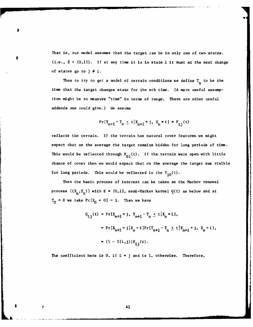
That is, our model assumes that the target can be in only one of two states.
(i.e., E = {0,1}). If at any time it is in state i it must at the next change
of states go to j 0 i.
Then to try to get a model of terrain conditions we define T to be then
time that the target changes state for the nth time. (A more useful assump-
tion might be to measure "time" in terms of range. There are other useful
addenda one could give.) We assume
Pr[T - T < tIX J, Xn i] = F t)+1 ij
reflects the terrain. If the terrain has natural cover features we might
expect that on the average the target remains hidden for long periods of time.
This would be reflected through F 0 1 (t). If the terrain were open with little
chance of cover then we would expect that on the average the target was visible
for long periods. This would be reflected in the F10 (t).
Then the basic process of interest can be taken as the Markov renewal
process {(X,T)) with E {0,1}, semi-Markov kernel Q(t) as below and at
T = 0 we take Pr[X0 01 = 1. Then we have
Qij(t) Pr[X+l-J, Tn+l-T n< tXn -i1
=Pr[Xn+l=jIX=i]Pr[Tn+l-T n < t lX n+ l -j, X=i],
= (I- I(i,j))Fij(t).
The coefficient here is 0, if i j and is 1, otherwise. Therefore,
41
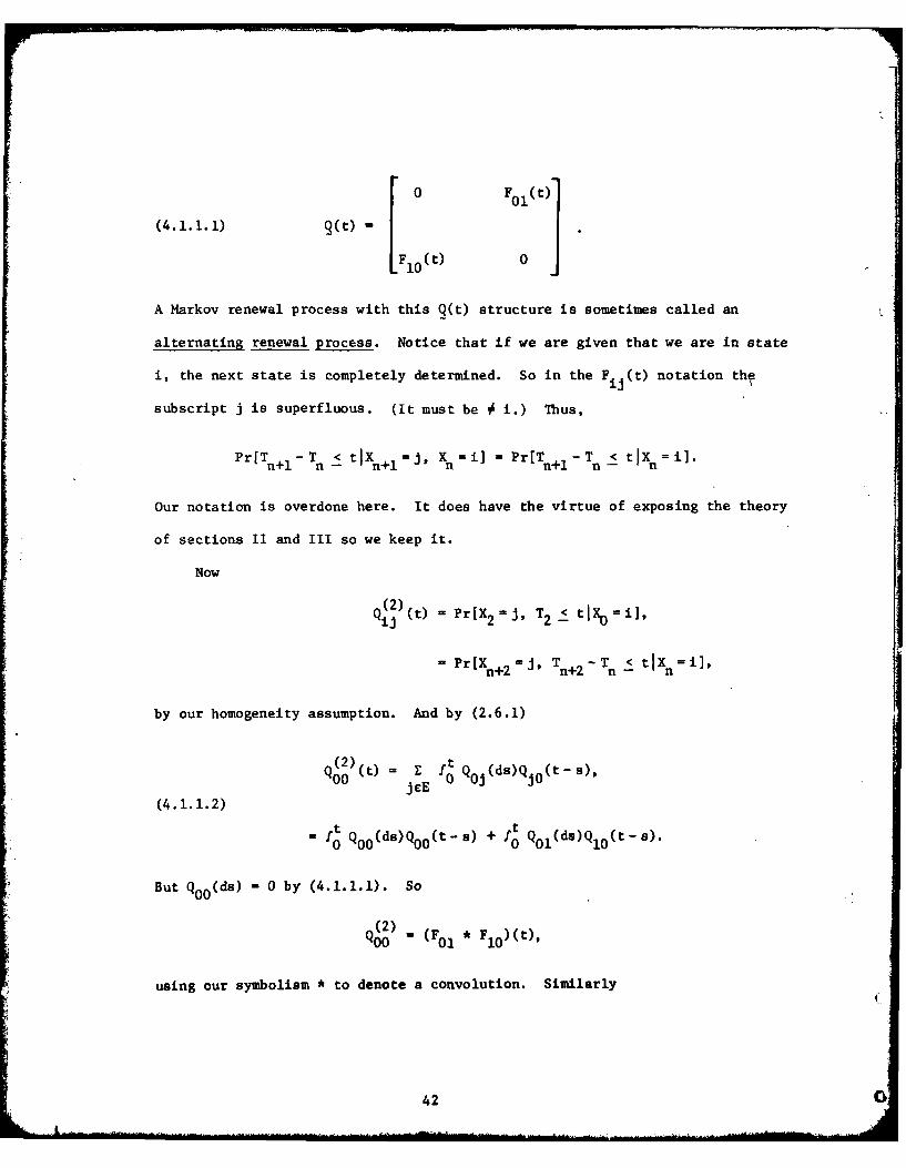
A Markov renewal process with this Q(t) structure is sometimes called an
alternating renewal process. Notice that if we are given that we are in state
i, the next state is completely determined. So in the FijWt notation the
subscript j is superfluous. (It must be 0 i.) Thus,
Pr[T -T < tjx J, X =i] -Pr[T -T < t jX=i].n+l n - n+l n n+l n - n
our notation is overdone here. It does have the virtue of exposing the theory
of sections II and III so we keep it.
Now
(2)2
- Pr[Xn+2 =j, Tn+2 -T n< tXn i],
by our homogeneity assumption. And by (2.6.1)
Q =2 t E f t Q (ds) Q(t -s),00 JcE j
(4.1.1.2)
ft Q Q(ds)Q00(t -s) + f t Q0 1 (ds)Q 1 0 (t-s).
But QOO (ds) -0 by (4.1.1.1). So
Q (2 (F0 1 F 1 )(t),
using our symbolism *to denote a convolution. Similarly
42

Q(2)M 0
* -- i, (t) ... 0
since either Q11 (t) or Q00(t) is zero when one uses (4.1.1.2) to compute.
Then it follows from these results that if the process starts in state 0,
the ensuing entrances to state 0 ("invisibility") form a sequence {S I andn
{Sn+ 1 -Sn I is a sequence of independent, identically distributed random
variables with
(4.1.1.3) Pr[Sn+I -S n < t] = (F0 1 * F10 )(t).
That is the process of successive entrances to state 0 (for the process start-
ing in state 0) is a renewal process with intervals distributed as in (4.1.1.3).
Suppose the target is invisible at t = 0. We would be interested in
knowing many things about it at some future time. For example we might want
to know the probability that the target is visible at some time t. More
importantly in order to attack it when it is visible, it is important to know
how long it will remain visible. Considering that it takes time to lay a
weapon on a target, if the target is not visible for a long enough time we
simply cannot destory it.
To get at such a problem as this, define a process {Y(t)l so that
Y(t) = X, if Tn < t < Tn+ 1
Then for each t, Y(t) simply tells us that the target is or is not visible. Also
define
Z(t) = Tn+l - t, Tn < t < Tn+l.
S 43

Then for each t, Z(t) tells us how long the target will remain in whatever state
it occupies at t. We will not stop here to prove that {(Y(t), Z(t))) is a semi-
regenerative process with F = {0,1} x R+. It is.
For A = {j} x {(y,-)} : F, define
(4.1.1.4) Gi(j,y,t) = Pr[Y(t) -J, Z(t) > y1X 0 f i],
(4.1.1.5) hi(J,y,t) = Pr[Y(t) = J, Z(t) > y, T > tjX 0 = ii.
(4.1.1.4) contains the information we want. For if j = 1, then that formula
will yield the probability that the target is visible at t and will remain
so for more than another y minutes given that originally the target was
invisible. (4.1.1.5) is simply the initial function of the {(Y(t),Z(t))} as
required by formula (3.3.1). But hi(j,y,t) can be easily found from the basic
{(X ,T)} process. For example, given that X = 0 we will have Y(t) - J, withn9
probability 1 if j = 0 and with probability 0 otherwise when T > t. Further-
more, Z(t) > y and TI > t if and only if there has been no change of state
before t (and thus' at t, Y(t) - 0) and there will be no change of state for
more than y time units after t. In general,
Pr[Z(t) > y, T1 > tjX 0 = i ] - Pr[IT > t + yjX 0 i l - I- F i(t +y)
where I - Fi(t+y) - 1 - E Qij(t). Altogether then,JE
Pr[Y(t) = J, Z(t) > y, T > tjX 0 = i] - I(i,j)[l - Fi(t+y)].
Then from (3.3.1) we put the pieces together as
44 C"

G =J~y~t) I(ij)[l - F (t+y)t + Qik(ds)GX(j,y, t- s)
and from (2.7.1) we have
(4.1.1.6) Gi(j,yt) = $0 R (ds)(1 - F.(t+y-s)).
Here Rj(t) is the i,j term of the Markov renewal function of the under-
lying {(Xn,Tn)} process. In general the Rj (t) function is difficult to
compute. But from the very special structure of this Q(t) matrix it is rather
simple for this problem.
0 F61(aQ*(a) =
F* (az) 0
where
F*j (a) = f O e-atFij (dt).
And using (2.6.6), it is easy to see that
1 Fol(a)F* (a) 1 - (a)F*o(a)
(4.1.1.7) R*(a)
FO (a)
1- F* (a)F o(a) 1- Fo(a)F-o(a)
At this point we can proceed in several ways. We can formally invert
45

(4.1.1.7). Once the functions F ij(t) are given (as in our example below),
of course, R(t) can be found by inverting R*(c) term by term and then using
(4.1.1.6).
Alternatively, one can view (4.1.1.6) as the convolution of two functions
and using the convolution properties of Laplace-Stieltjes transforms, the
transform of the solution can be obtained immediately from (4.1.1.6) and
(4.1.1.7).
Because R(t) has some independent interest, we will proceed to our
example, following, along the first of these two paths.
An example may make the manipulations involved here more apparent.
Example.
Fol(t) F1 0 (t) e - b t
Then
bi
F ba - w* (0F01() -+ -j F10()
Then it is easy to see that
) 1 -b 2/(b+) 2 b
from (4.1.1.7). This matrix of transforms is not hard to invert. One does it
term by term to obtain
46

1, if t = 0,
R0 0 (t) R1 1 (t) =
bt 1 -2bt
R01 (t) = R10 (t) = 2 + 4 [1 - e t > O.
It should be noted that RWi(t) will always have a jump at the origin of size 1
since we have defined this function on the closed interval [O,t] and assumed a
jump occurs at t = 0 (i.e., T = 0). Thus, the expected number of visits to
state i is always at least one if X = i.
Then from (4.1.1.6) we have after a bit of algebraic manipulation
1 by 1 -2bt -by(a) G0 (O,y,t) e- e
(4.1.1.8)1 -by 1 -2bt -by
(b) Go(l,y,t) = e - e
In interpreting (4.1.1.8) we have that, if the target is hidden initially,
it will be hidden at t and will remain hidden for more than y more time units
with a probability given by (a). On the other hand, if it is hidden at t = 0,
it will be visible at t and will remain visible for more than y time units
with probabilities given by (b). One notes that
(4.1.1.9) Go(O,y,t) + Go(l,y,t) = e- b y > 0
as it should for this is simply the probability that the time until the next
change of state is greater than y no matter what state is next occupied. Since
state occupancy times are identical exponentially distributed random variables
47

(4.1.1.9) is a consequence of the forgetfulness property.
If in (4.1.1.8) we let y 0 then
Gi(J,O,t) Pr[Y(t) - JX O = i].
Therefore this limit is the time dependent state probabilities for {Y(t)}. If
then we let t , we obtain the "steady state" probabilities for {Y(t)}. Of
course these probabilities are each 1/2 because of the symmetry we have built
into the problem.
Since
1 -by 1 -2bt- byG0(l,y,t) = Pr[Y(t) =1, Z(t) > y 0 ] = - e - e,
and
G0 (l,0,t) Pr[Y(t) f1X0 - i] (1 e-2bt),
we have
Pr[Z(t) > yIY(t) = l, X 0 ] _ eby (1 -2bt)/1( 1 - e 2bt
- e-by, for all t> 0.
Finally, since Pr[X 0 0] - 1,
Pr[Z(t) > y1Y(t) - 1" e-1, for all t > 0.
Of course, this is expected because of the forgetfulness of the exponential
distribution. The point is that the left hand side is one of the sought for
probabilities. It is the probability that the target remains visible for
more than y more minutes given it is now visible. The simple result follows
48 (

from the very special assumptions made about F ij (t).
Because of the simplicity built into this example in an attempt to provide
a model that easily exposes the concepts of sections II and III, the problem can
be solved many (and easier) ways than we have done. The {Y(t)) process is a
Markov process and those topics can be used here. The {(X ,Tn ) process is an
alternating renewal process and those methods can be used here.
4.1.2. Departures from the M/G/l/N Queue. Let us return to the example
of section I to see why our variance estimates differed from the "true"
variances. There, recall, we were interested in an M/M/l/3 queue and its
departure process and in particular its mean and variance. We have seen in
section 1.1 that one can use simple arguments to obtain the mean value (formula
(1.1.1)). The variance is a different matter.
To start let us define
Xn = the queue length left behind by the nth departing customer,
n
T = the time of the nth departure.n
While our results will be true for many queue disciplines (but not all) we will
fix our attention on a first in - first out discipline.
The increment (Tn+1 -T n ) is the time between the n+l and n departing
customer. Clearly, this increment satisfies the identity
Sn if X > 0
(4.1.2.1) T n+l-T -
I + s if X-.
That is, the time between two consecutive departures may be one service time
5 49

(of customer n+1 which we have denoted as S This occurs if the queue
left behind by the nth departure is at least 1. On the other hand, this inter-
departure time will be the total time spent awaiting the next customer (I) and
then serving him (Sn) if the nth departure leaves the system empty.n+l
The identity 4.1.2.1 has been known as one of those folk theorems in
queueing for many years. However, its exploitation awaited a development
of Markov renewal theory.
Now, from that identity, we have immediately
(4.1.2.2) Pr[Tn+1 - Tn < tiX J] - 1 - e- pt , j- 1,2,'.-,
where the right hand side is simply the probability that a service time is
less than or equal to t. (Remember in M/M/l queues service times are identically
distributed. n plays no major role here.)
Also,
(4.1.2.3) Pr[Tn+I T < tIX n 01 t [1 e- (t s) ds
which simply says that Tn T- < t given X 0 if and only if I + S < t.whc sml sy ta n+ 1 Tn- n n-
The integral on the right is the convolution of the distributions of I (an
exponentially distributed random variable with parameter A) and S (ann
exponentially distributed random variable with parameter 0). As is usual in
queueing theory we have assumed the arrival process and service time process
are independent processes.
We further know from first principles of queueing theory that {X } is a
Markov chain and
50

t(4.1.2.4) PrXn+i -JiIX =0 Tn+ -T =t ti e for J-0,1,2,
= -(At)~ Ji+le At
(4.1.2.5) Pr[X+ 1 =jI X i, T nl -T n j (J-'i+l) 1 2 >ji - 1i, i'> 0.
Since N = 3, the maximum queue that can exist at a point of departure is 2.
Note, therefore, that this {(X nT n)1 does not give, directly, the queue
length process that one would obtain from the usual Markov chain analysis of
1this problem for all t > 0.
(4.1.2.6)~~C PrXJ i -£)i+l -t i 0
(4.1.2.6) Pr[X =21X =0, T -T =tj W _ (Xt) e i 0
n+l n n+1 n -2 J
Then putting (4.1.2.4)-(4.1.2.7) together with (4.1.2.2), (4.1.2.3) we obtain
the semi-Markov kernel as
0, if i,j = (2,0)
ft (Xz) Ji e-X (petie )dz, (i,j) c{(,)ll,2l)0 (j-i+l)!
f t (Xz) e XZ [1 -e- X(t z) ](lielz ) dz, (i, J) e {(0,0) ,(0,1))
(4.1.2.8) Qij(t) = 0 ji e
t= (Z (k-i+)e! X JA(e1Z)dz, (i,j) c {(,2),(2,2))
t (Az) k -Azi -- A(t-z)-~eaz~d,(~)-02
k!2 0 k!
1 See the discussion on state spaces in section 4.1.3.
# 51

In this way we can establish our first result as:
The {(Xn,T)) process is a Markov renewal process on E' {0,1,2}
with semi-Markov kernel Q(t) whose elements are given by (4.1.2.8).
The identity 4.1.2.1 establishes that T l-T n depends only on X . Formulas
(4.1.2.4)-(4.1.2.7) establish that Xn+1 depends only on Xn and T +-Tn.
Formula (2.2.1) establishes that {(X ,T )) is a Markov renewal process. Thatn n
the transitions functions are as given requires the arguments that produced
(4.1.2.8).
The Markov chain {X I is the usual Markov chain embedded at departuren
points. From the theory of queueing (or directly by letting t - in
4.1.2.8) we find the one step transition probabilities for the {X n process
to be given by the Markov matrix:
14-p (1+p) 2 (1+p) 2
2
l+p (l+p) 2 (l+p) 2
1 p0 l+p 1+p A
n
Since we need (n) below it is necessary to determine Pn. This can be
done easily for this problem using an eigenvalue analysis. We have done
that. The eigenvalues are respectively
X0 l , = P/(l+p' 2 A 0,
52 0

The eigenvector matrices are
1 _1 _ p22 2 2l+p+p 1+ + l+p+p
S= 1 -p2 -p - (l+p) 1 12 2 2p(l+p+p) (1+p+p2) (1+p+p2)
1 (1+p) 1 i/p -1/p 0
That is,
Pn =S An S
for S, A, and S given above. From this one finds that w(n) converges to its
1 (pp 2) n"steady state values of 2 A +0, i 01,2. The b arel+p+p2 2ip I a b i
respectively (1+p __pp 2 p2l+p+p2 l+p+p2 'l+p+p2"
Now
(4.1.2.9) F(n) (t) Pr[Tn+l-T nt]= E E Pr[X+l-j, Tn+lT n<tiX_ ni]Pr[X nfiicE JiE
Thus if we take wi(n) Pr[X = i] to be the n step state probabilities for the
underlying Markov chain {X n (w(n) = i(0)Pn), (4.1.2.9) can be written in matrixn
notation as
(4.1.2.10) F(n) (t) = w(n)§(t)U, n =12,""
where (n) is the (row) vector whose elements are vi(n), Q(t) is the semi-Markov
I
D 53

kernel of elements (4.1.2.8) and U is a (column) vector of lVs.
Furthermore,
F (n) (t1,t 2 =Pr[Tn+ 2 --T +1< t 2 T n+1- T n< t
jEkcE PrXn+2 -J X+l -k, Tn+2 T +i < t 2 P T n 1 T<
or
(4.1.2.11) F ()(tt 2) w (n)Q(t I)Q(t 2)U, n = ,--
The probability distribution for any two intervals k transitions apart
is given in matrix form by
(4.1.2.12) F (n) (t l'tk) = i(n)Q(t1)pk-lQ( t)U.'
Then from (4.1.2.10)-(4.1.2.12) one can determine the means, variances and
autocovariance functions for any n. From this one finds
7r 0(n) 1a. E[T - T]- A
W 0(n)1(4121)b. VariT -TI- [2-iw0(n)] + 2'(4..2.3)n+l n Ix2029
c.~~~~ Coi (n)c.Co[Tn+2 T n+1 T n+1 T n 2 [11-AE(T -~lT n]
for the case M/M/l/3. Graphs of (c) are given on the following pages.
Covariances of lag 2 and 3 are given in table 4.1.2.1 for a few values of p.
It is instructive to note that the covariance of lag 1 (4.1.2.13c) is
always negative for the M/M/l/N queues (0 < N < m) Therefore the variance
54
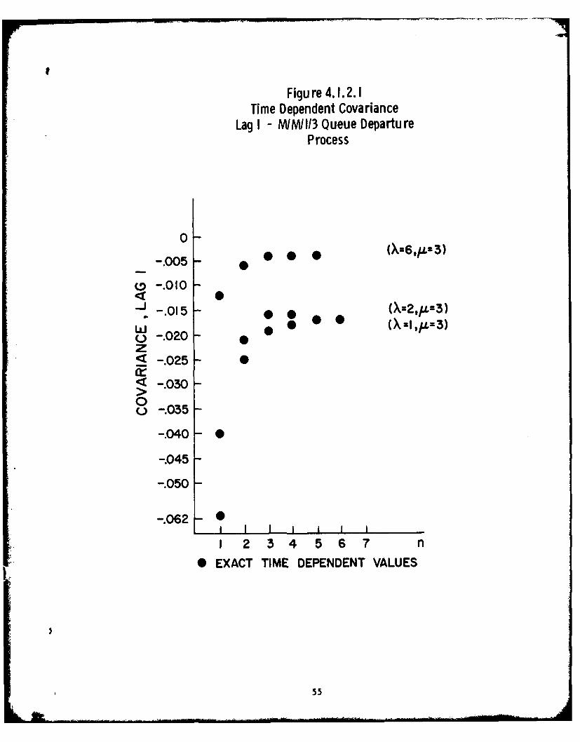
Figu re 4.1. 2. 1Time Dependent Covariance
Lag I -N 1/II3 Queue DepartureProcess
0
*.0 * -X6~t3
(~-.010
S-.015 - * (X 0u3w -02-00 (X:Iq~z3)
z!5-.025
-0300 o-.035
-.040 -0
-.045
-. 050
-.062
1 2 34 567 n* EXACT TIME DEPENDENT VALUES
55

Table 4.1.2.1
Covariances of Lag 2 and 3
for the M/M/1/3 Queue
Lag Covariance X-1, p=3 X=2, v-3 X-6, v-'3
2 /p2 + VA + A2 2 -.01775 - .01662 -.00453
2 2 2 2 23 -(PA) /(p +jPA+A )0+0) -00332 -.00398 -.00100
56
estimated under the assumption of independence (as was computed in section I
from the simulation) overestimates the true variance. The overestimate can
be relatively large. In the class of Erlang server queues, it can be shown
(Disney and de Morals (1976)) that the covariances can be positive,
negative or zero depending on X/V, N and the Erlang parameter. Therefore,
variances estimated under the assumption of independence can underestimate,
overestimate or correctly estimate the "true" variance depending on these
parameters: The key point to be made, however, is that the departure process
from the M/M/l/N queue is a Markov renewal process. This Markov renewal
process has {T n+ - T } as a sequence of independent, identically distributednl n
random variables in only 4 cases (Disney, et al. (1973)). Terms in this
sequence are dependent even in the steady state except for those 4 cases.
Thus, any statistical analysis which relies on independence of the random
variables is inappropriate to the analysis of this sequence. The problem
is caused by dependence not by distributional assumptions.
1
4.1.3. The Time Dependent M/G/l/N Queues. In this section we will
study the queue length process of an M/M/l/3 queue. Because of the
computations involved this is about as far as we wish to push our hand
computation talents. But one should be aware that the exercise here is
just that - an exercise. The methods illustrated by the exercise apply to
the M/G/l/N queue in general. inlar (1975) pursues the topic more generally
for the M/G/l case.
1There's a rather large literature on queueing applications. The reader
interested in this special case might consult [16], [17], [181, [19], and[201 in the Bibliography to start.
57

We have seen in section 4.1.2 that for the M/M/1/3 queue there is an
embedded Markov renewal process {(XnTn)) on E {0,1,2,} where X is then n n
queue length left behind by the nth departure and T is the time of the nthn
departure. The semi-Markov kernel Q(t) was given by (4.1.2.8).
Let
Z(t) = Xn, T < t < T l*
There is a question here of some interest. Since N = 3(< -), Xn 0 N
for any n except possibly n = 0. That is, the queue can never be full at
a departure point (almost universally we consider the queue just after a
departure.) Thus, in the limit the model {Xn) gives us no direct information
about the queue being full. The state X fi3 is a transient state. (In factn
once state 3 is left after n = 0, if it starts, there, it can never be reentered
in the {X ) process. If it does not start in state 3, the process can nevern
be there.)
However, if X = 2 for some n then Z(t) may be 3 (if an arrival occursn
before the next departure). Thus the continuous time process may occupy state
3 even though the embedded process never does after the process is started.
Thus, we take F - {0,1,2,31.
Then {Z(t)} is the time dependent queue length process. It is easy to
check conditions (3.1.1-(3.1.3) to see that {Z(t)) is a semi-regenerative
process. Then if we let A {j) for j = 0,1,2,3 we have
58

e- Xt, (i,j) = (0,0),
O t -X(t-s) -us (Os) k-1si Xr f Ae e -) e ds, (i,j) (0,3),k=2 k-i
(4.1.3.1) hl = 2t) ,00. (i,j) 0 , ,p j-i -Xti~ e ,(i J) c { (I, 1),(1, 2) ,(2,2)}
O (Xt) e t
k . (i tk! e - , (i,j) c {(1,3),(2,3)1,k=3-i
eivt, (ij) = (3,3),
0, otherwise.
For example, if i = j = 0, then the queue is empty and the first departure
(after the previous departure) has not yet occurred if and only if there has
been no arrival in [0,t]. This accounts for the first term in (4.1.3.1). On
the other hand, i = 2, j = 3 then at T the queue has 2 customers and at tn
(which occurs before the next departure) the queue has 3 customers if and only
if at least one customer arrives in [0,t] and the server does not finish the
customer he began at T nn
The queue length process {Z(t)) is a semi-regenerative process with state
space F - {0,1,2,3} and the underlying Markov renewal process {(X n,T n)} of
section 4.1.2. For the {Z(t)} process one has
hi(Jt) - Pr[Z(t) = J, Tn > tIX - i]
as given in (4.1.3.1). Furthermore, the continuous time probability paths
59
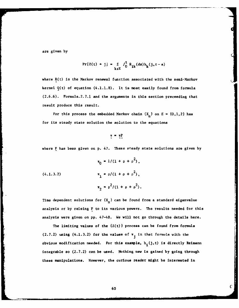
are given by
Pr[Z(t) J -J E fo Rikds)h
where R(t) is the Markov renewal function associated with the semi-Markov
kernel Q(t) of equation (4.1.1.8). It is most easily found from formula
(2.6.6). Formula-2.7.1. and the arguments in this section preceeding that
result produce this result.
For this process the embedded Markov chain {X n on E - {0,1,2} hasn
for its steady state solution the solution to the equations
ir = liP
where P has been given on p. 47. These steady state solutions are given by
O= 1/l + P + P2),
(4.13.2)ir 1 = p/(1 + p + p2 ),(4.1.3.2) 1 R +P+1
2 2'T2 p/( I + P + p2).
Time dependent solutions for {X n } can be found from a standard eigenvalue
analysis or by raising P to its various powers. The results needed for this
analysis were given on pp. 47-48. We will not go through the details here.
The limiting values of the {Z(t)} process can be found from formula
(2.7.2) using (4.1.3.2) for the values of wj in that formula with the
obvious modification needed. For this example, hi(J,t) is directly Reimann
integrable so (2.7.2) can be used. Nothing new is gained by going through
these manipulations. However, the curious reader might be interested in
60 C

II
comparing the {X } and {Z(t)} limiting values.n
This problem can be solved other ways, of course. But our methods have
the virtue of exposing the structure of the problem and showing vividly where
the difficulties are coming from in the computation of time dependent solutions.
The matrix of distributions for Pr[Z(t) = J, T1 > tIX0 = ii causes some problems
but it has some redeeming features. Rather the computational problems are
coming primarily from the convolutions of Q(t) necessary to generate R(t).
Whether these problems can be surmounted by a careful numerical analysis or
not is beyond our ken. The important observation is that we have pinpointed
the problem that ultimately must be tackled. The same problem arises in the
study of time dependent solutions for the state probabilities for M/G/1/N
and GlI/M//N queues. However, these computational problems exist no matter
how one tries to solve the time dependent problem. As always these problems
satisfy the well known conservation of difficulty law.
4.1.4. A Disease Model. In the disease model of section 3.2.3 we started
by assuming the disease could be modelled as a Markov renewal process. There
was little hard data at that time on which to base any assumption about the
stochastic nature of the evolution of the process. The assumption of Markov
renewalness was made simply because we thought it would be a good first
approximation and because it seemed clear from discussion with people more
knowledged in the process than we as operations research people were that
sojourn times in the various states of the disease depended on both the current
state and the next state to be visited. If later data proved the process was
Markov we had not lost time or analytic capability. If later data showed that
the process was not a Markov renewal process, the Markov renewal assumption at
61
least directed our attention to what data was needed in what form - a not
inconsiderable accomplishment by itself.
At the time of this study there was some question as to whether the
disease was regressive or not (i.e., could return to a state it had already
visited). Models of both regressive and non-regressive diseases were studied.
We will discuss here only the non-regressive model because of its simpler
stochastic structure.
Because lifetimes are finite we consider the disease as starting in some
state 0 which can be taken to be "the disease absent". The disease may then
pass through its several stages which we will simply call stages 1,2. (In the
real study there were more than these two stages but to keep the discussion
simple we will keep just two.) At any stage (0,1,2) the disease can enter an
absorbing state 4 to denote death from causes other than this disease. From
stage 2, the disease may also enter an absorbing state, state 3, to denote
death from this disease.
The ultimate aim of the study was to try to determine when and how often
a person should be examined for this disease and its progress over time. For
our present purposes, we will simply look at a few properties of the model
of the disease. The other questions take us too far afield and require the
development of too much more machinery than we can accomodate in these notes.
To set up the problem formally, let {(X ,T)) be a Markov renewal processnn
on the state space E - {0,1,2,3,4}. Let X - j if, at the nth change of state,
the disease enters state J. Transitions occur from j to J + 1 or 4 (the
disease is not regressive). State 3,4 are absorbing states. Let T be then
time of the nth transition. T - 0, X - 0 are the initial conditions to imply
62

that one is born free of this disease. ('11iis is not a crucial assumption. We
could just as well take T0 = 0, Pr[X j] J
Then, we let
Pr[Xn+IsJIX n iI = P j' i,j E,
and let P be the matrix of these Pj" Then P has the form
0 Po1 0 0 P04
0 0 P12 0 P1 4
P 0 0 0 P2 3 P2 4
0 0 0 1 0
0 o 0 0 1
so that by our modelling procedure P is upper triangular. There are two absorbing
states and transitions are as shown under the assumption that the disease is not
regressive.
Then, let
F ij(t) - Pr[T+I - T < tIXn+lI J, Xn i], i,j E E.
Then, using (2.2.2) we have that the Markov renewal process {(XnT) has semi-
Markov kernel given by
63

0 P01F6, 0 0 F(t)0 PO Ol 04 04
0 0 p F(t) F012 12 14 14
F(t) F(t)0 0 0 P2 3 2 3 P24 24
o 0 0 F(t) oa33
0 0 0 0 FM44 _
Except for the last 2 rows, we can interpret the non-zero elements here as
telling us that at the nth change of state, the disease moved into state i.
In at most t tim units it will change state again and thence will move into
state j. The last two rows require a bit of discussion. These rows correspond
to the absorbing states 3,4. From either of these states transitions to any
other state is impossible. This explains the O's in the row except for the
diagonal term. Transitions from the state to itself occur at each step with
probability 1 (as is true for any Markov chain model with absorbing states).
However, the time from first entry to these states to the next transition is
finite with probability 0. Thus Fij(t) = 0 for all finite t > 0 and
F33 (o-) = F 44( ) 1. So, in effect, once states 3 or 4 are reached the process
stops.
For diagnostic purposes and treatment one would like to know for any
t > 0, the stage of the disease, how long the disease has been in that stage
and how much longer that stage will be occupied. These three variables are not
independent so knowledge of the probability of the triplet will be more
informative than knowledge of the marginal probabilities of each. Therefore
we define
64

Y(t) = X, if T< t < Tn+
(4.1.4.1) U(t) - t - T, if T < t < T
V(t) - T+1 - t, if Tn< t < T+l"
(It should be noted, as is well known in renewal thoery, V(t) + U(t) Tn+I- T
n
does not have the distribution Fij(t). Thus, for example, one cannot directly
use V(t) + U(t) to estimate F ij(t) from data.) Let Z(t) = (Y(t), U(t), V(t)).
Then {Z(t)} is a three-tuple valued random process on the state space E xR+x R+.
This process carries the information we want.
Now it is clear that (Tn I are stopping times for {Z(t)). (For example, see
section 3.2.1.) Furthermore, Xn is completely determined by Z(t) for t < Tn
In fact X is simply Y(T ). That {Z(t)) satisfies condition 3 of section 3.1 isn n
not as clear. We will give a heuristic argument that it does. Notice first of
all that at each Tn, U(T) = 0 and V(T)n is the time until the next transition
starting in state XT . Furthermore, Y(t) for all t > T has probability lawsn
determined by XT by (4.1.5.1). Thus, (Y(t), U(t), V(t)) is probabilisticallyn
determined by XT for t > T. Since the {(X ,T )) process is homogeneous,C
these probabilities do not depend on n so we can take n - 0. Thus, condition
3 of section 3.1 is valid and {Z(t)} is a semi-regenerative process.
Let A = {Y(t) =j, U(t) >x, V(t) >y} denote the event "the disease at time
t is in state j, it has been in this state more than x time units and it will
remain there more than another y time units." Let
f0(A,t) - Pr[Z(t) c A 0 - 0].
Let
h0 (A,t) - Pr[Z(t) c A, T1 > t12 - 0].
* 65

Then
(4.1.4.2) h 0(A,t) =I(0,J)I (x.-) (t) Pr[T1 > t + yIX 0 01.
We can explain (4.1.4.2) as follows. The condition T 1> t means that the
disease has not changed states by t. Therefore, for Z(t) to be in A it must
have started in A (i.e., X = 0) and not moved out of that state (hence, J = 0).0
No other circumstances have T 1> t. Thus, here, Z(t) e A only if A
{0, U(t) >x, V(t) >y). But there's more. Z(t) will be in A only if t C (x,-).
The indicator functions I(0,J), I (x-) (t) correspond to the probabilities for
these observations. And finally, V(t) > y only if T> t + y. Let
90(t + y) =Pr[T 1 > t + yIX 0 0].
then
90t+ y) = 1- E Pr[Xl = J, Tl. t + yIX 0 =0].
Thus, we have
Pr(Z(t) c A, T 1 > t1X0 - 0].
Then since (Z(t)) is a semi-regenerative process we have from (3.3.1)
f (A,t) - h (A,t) + E 't Q(ds)fk(A.T- a),0 0 ~keE f ~
and f rom (2. 7.1)
fi(A,t) - E ft Rij(ds)h.k(A~t- a)
where R is the Harkov renewal function for Q(t).
66

Because of the special structure of Q(t), the computation of R(t) is
simple. In fact, because of the several assumptions made here (primarily
the lack of a regression in the disease), there are several other ways this
problem could have been solved. Because of the structure of the problem
and the ability to easily generalize it to account for more states, different
transitions or regression we think it is preferrable to other models.
Then h i(A,t) is Riemann integrable ( it is a probability function) and
hence if necessary one can use (2.7.2) to determine the limit of f0(A,t) for
t - -. Of course, because {Xn I is an absorbing Markov chain this process
eventually ends in states 3 or 4 with probability 1. However, for disease
control it might be important to know which of these absorbing states has the
larger probability of eventual entry so there is some value in computing the
limiting probability.
There is nothing new to be gained by going through more detailed calcula-
tions here. The intent of the example is simply to show how one could model
a process as a Markov renewal process and use the results for controlling the
process. Details of calculation have been provided in previous examples.
It should be mentioned that there was some argument that this particular
disease did not have a stationary transition mechanism. Case studies were
inconclusive. Some seemed to support the assumption of homogeneity, some did
not.
Therefore, this disease was also modelled as a full, two dimensional
Markov model with (Xn, T) as before, but now it was assumed that
6
* 67

Pr[Xn+l'ij, Tn+ 1 < tX ni, Xn1 l'''X O, Tnfy, Tn1 l,"',T O]
- Pr[Xn+l-J. T,+l < tX ni,T =y.
In this way the next stage of the disease and the time at which that stage
is reached (not the interval between the nth and (n + l)st jump) depends
on the current stage and the time at which that stage was reached. This
model is a Markov model on E x R+. While it is appealing at first glance,
one wonders how enough data would ever be collected to estimate the above
probabilities so as to validate the model.
The principle here seems to be that we are concerned with modelling.
The model that cannot conceivably be validated (not necessarily with today's
technology, however,) may well be useless. In short, the cry for "realistic"
models can often be detrimental to modelling.
There is one more afterword of some importance here and in other models.
In this model one must obtain some estimates of Qij(t) either directly or by
estimating pij and Fij (t). At the time this research was done such estimates
were not available. Therefore, one could proceed parametrically by proposing
likely Pij and Fij(t) to observe the sensitivity of the {Z(t)} probabilities.
If these probabilities (or more likely moments obtained from these probabil-
ities) are not sensitive to reasonable values of these parameters then it
does not seem reasonable to spend effort getting precise estimates for the
purpose of this model. If on the other hand the derived information is
sensitive to the parameters then one must have precise estimates. In that
case the model is useful in determining what data to collect and analyze. There
is no virtue in collecting "all possible data" in the hopes that it will be
68
useful. It often is not and the data collection and analysis study then is
not only useless but expensive. That is, it seems to us that a researcher of
real life problems should have some model in his mind before extensive, costly
data collection is begun. Of course, one often needs a preliminary study to
suggest such a model.
4.1.5. Police Emergency Calls. Nearly every community in the country must
supply public medical emergency service for its citizens. How a locality does
this varies. In Detroit in 1968 such service was provided through the police
force.
In the Detroit system of 1968 police precincts, which act as nearly
autonomous units, had a mixture of sedans and station wagons used as police
vehicles. The sedans were always used for the normal duties of police work
such as patrolling. These sedans were called "squad cars". The station
wagons manned by police served a dual role. Their normal duty was to act in
a squad car capacity. However, these station wagons had some medical
emergency equipment so that if necessary they could act as an "ambulance".
Whenever a medical emergency arose in a precinct, a citizen could get ambulance
assistance from these police ambulances.
For many reasons, the city decided to take a look at this dual functioning
police-ambulance system in 1968. The results of our part of that study are
contained in a long report (Hall (1968)) that contains the details of the
following analysis, it's use in a rather sophisticated analytic model which we
cannot reproduce here and the conclusions drawn from this model. The purpose
of the following section is to show how the foregoing study of Markov renewal
processes was used in one place (it was actually used in several places) in
* 69

our study of the dual functioning ambulance system in Detroit in 1968.
After a rather extensive period of observation of the system and many
discussions with personnel intimately aware of the details of the system
it was possible to develop a crude model depicting the major components
of the system. The precinct contained a number of squad cars (the exact
number is not important to our later discussion) and one or two ambulances
(again exact numbers are not important here). Telephone calls triggered a
dispatcher to dispatch a vehicle to some location in the precinct. Based
on information available from the call the dispatcher sent the nearest
squad car (sedan or "ambulance") for police assistance or an ambulance to
the call for medical emergency assistance. The intuitive rule used by the
dispatcher was primarily to send to a call for police assistance the vehicle
assigned to patrol the area from whence the call arrived. (These areas were
called "beats.") In the event the normal vehicle was not available (perhaps
it was on another call), the nearest available vehicle in the precinct was
dispatched. In this part of the system squad cars and ambulances were
indistinguishable.
If the call arriving to the dispatcher was for an ambulance, the nearest
ambulance was dispatched. This meant that the beat normally patrolled by that
ambulance, when acting as a squad car, was unpatrolled during the time the
vehicle was acting as an ambulance.
The driving force of this system was the sequence of calls received by
the dispatcher. Rather than delve into the details of the dispatcher himself
and our models of him or the process of vehicle dispatching and response and
our models of them, we will limit ourselves here only to one aspect of the
70

process of demand - the time sequence of calls.
To study this sequence, data were obtained on over 5000 calls received by
the dispatcher in one precinct in one month. Because these calls are immediately
recorded by the dispatcher and punched on a clock to record time and date, this
data was about as clean as one can expect to get from any real life system.
(Such was not the case in our study of other parts of this system.) One
problem with the data was that it included a holiday which was obviously not a
typical day. The analysis tried to correct for that.
By collecting data for one month only, in one precinct, of course, it is
not possible to discuss the behavior of the system over the year. (e.g., one
would expect data collected in summer months to be rather different from data
collected in winter months and our study cannot reflect that difference.)
Furthermore, you may recall that 1968 may not have been a typical year for
police work in Detroit. Our data cannot reflect that. Therefore, whether the
detailed numbers of the following discussion are valid for every month of every
year or every precinct is a moot point. The analysis of the data and the over-
all model, however, are probably useful for more general studies and the
following is presented in that spirit.
The total calls received by the dispatcher were first split into police
calls and ambulance calls. Each series was analyzed separately to start.
We will pursue the ambulance data briefly in the following. The police data
exhibited somewhat different behavior that would require a much longer
discussion than this example deserves as an example of Markov renewal modelling.
First the total number of ambulance calls per day were plotted for the
period of study (see figure 4.1.5.1) and then were broken into three sub series
* 71

0
-(
0
to )i N83d STIVO-40 81 1wn
72U

for each of the three shifts of police work. (See figure 4.1.5.2.) No obvious
trends were observed nor were there any noticeable shift to shift variations.
(The police data differed here.)
Based on the above preliminary analysis, times between ambulance calls
were computed and subjected to a battery of tests available in a statistical
package for time series analysis then available for computer analysis. This
package computed for us the usual means and variances of the interevent times.
More importantly for modelling, however, it computed auto-covariances. We
computed these for lags up to 100 and, using the usual large sample theory of
these covariances, we came to the conclusion that the ambulance data were from
a renewal process. (i.e., the covariances were all essentially 0.) This
result is not surprising. One expects emergencies to occur "randomly" over
time and therefore exhibit properties of renewal processes. But this does
not mean that calls for ambulances in the police system (which is what is
under observation here) should obey such a process. Road accidents involving
multiple victims might well introduce non-renewal properties into the process
of calls for ambulances. What the data seemed to indicate is that, if such
properties exist for real they occur so seldom that over the course of the
entire data record we had, they could not be exposed by the methods used in
the data analysis.
To double check the correlation results the periodogram of the data was
estimated. Again, using standard statistical tools and the available computer
routine, this analysis supported the renewal assumption of the correlation
study. (See table 4.1.5.1.) Based on these results and our intuition we pro-
ceeded under the assumption that the ambulance call process was a renewal
73

CDC
0-
-(N
U.LL LA-m,)m x
qb)
OD
ocJ
-dli
OD -D v cl
1-41HS~I~ 83 'a-.O83vn
740
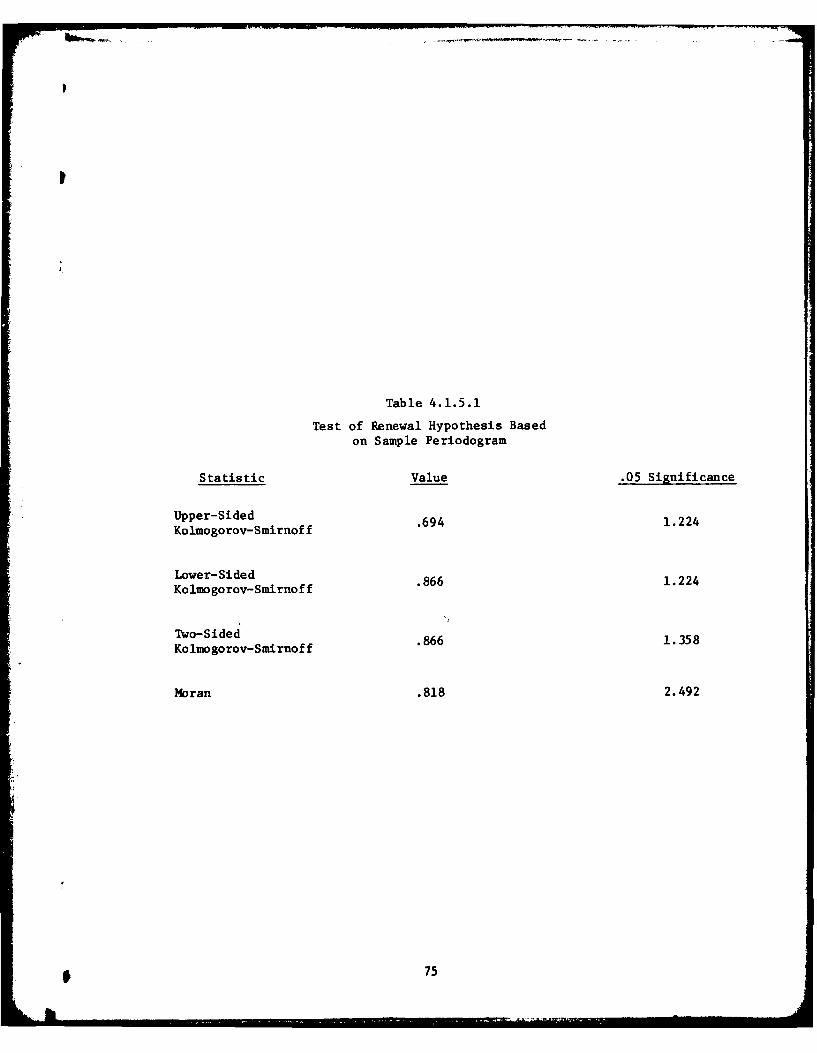
Table 4.1.5.1
Test of Renewal Hypothesis Basedon Sample Periodogram
Statistic Value .05 Significance
Upper-Sided .641.224Kolmogorov-Smirnoff .9
Lower- Sided .6 .2Kolmogorov-Smirnoff .6 .2
Two-SidedKolmogorov-Smirnoff .866 1.358
Moran .818 2.492
75

process.
Since an ordinary renewal process is characterized by a single probability
function, the remaining task was to analyze the data to estimate this function.
There are many tests for goodness of fit of data to distributions. We used
five and found that for the precinct under consideration an assumption that the
data satisfied the hypothesis of a Poisson process had to be rejected. (i.e.,
the interevent times form a renewal process - which we accepted - and these
interevent times are exponentially distributed - which we had to reject at
this point. (See table 4.1.5.2.)) The Moran test (one of the five goodness of
fit tests failed by the data) has high power against a gamma distribution
alternate hypothesis, so an attempt was made to fit a gamnma distribution to
the data. This attempt was successful using different methods to test the
goodness of fit. (We also used a hypothesis test that is designed to be
powerful against a log-normal alternate hypothesis.) The gamma density
function is given by the formula
k
kk k-1 -kx:f(x) =()x k - e-kX/I/r(k), k > 0, > 0, x > 0.
Based on all of the above analysis then we used maximum likelihood
estimators to estimate the requisite parameters of the gamma distribution.
Table 4.1.5.3 gives the maximum likelihood estimates of k and V. Then we
had a complete picture of the arrival of telephone calls to the dispatcher
for medical emergency service. But we were not out of the woods yet.
The objection was raised that even though the calls for ambulance
assistance seemed to be a renewal process with gamma distribution intervals
there was no evidence that this process and the process of calls for police
76
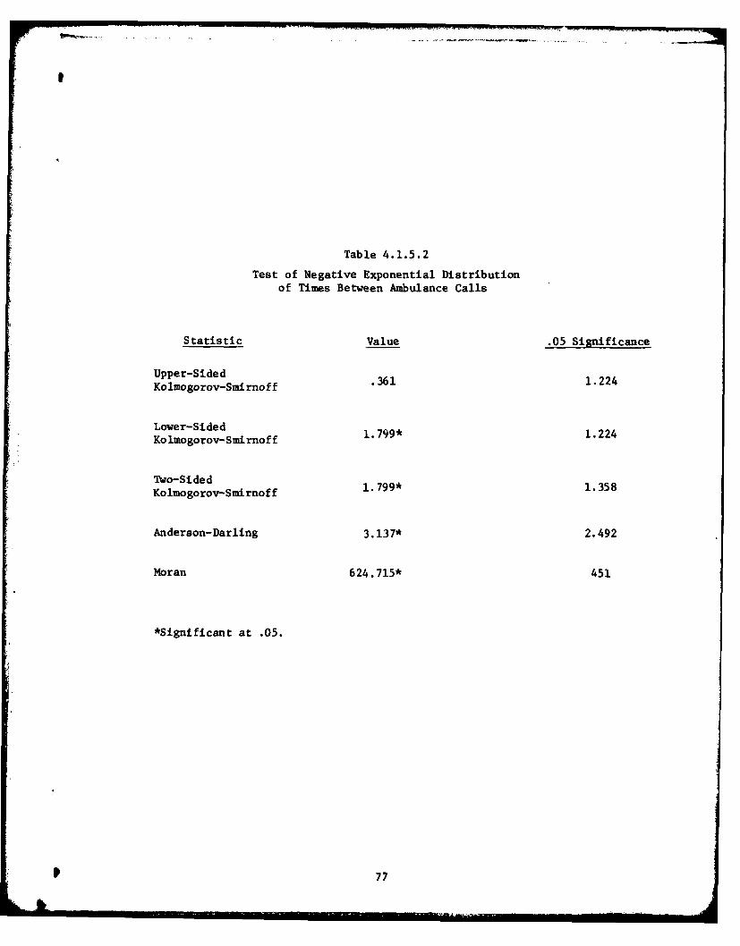
Ii
Table 4.1.5.2
Test of Negative Exponential Distributionof Times Between Ambulance Calls
Statistic Value .05 Significance
Upper-SidedKolmogorov-Smirnoff .361 1.224
Lower-SidedKolmogorov-Smirnoff 1.799* 1.224
Two-Sided
Kolmogorov-Smirnoff 1.799* 1.358
Anderson-Darling 3.137* 2.492
Moran 624.715* 451
*Significant at .05.
77
~IJ~i

Table 4.1.5.3
Maximum Likelihood Estimatesof Parameters for Gamma Model
of Time Between Ambulance Calls
101.2
k .77
Coefficient 1/2 1.14of Variation (k
78

assistance were independent processes. Thus, so it was argued, we could
not model the demand on the dispatcher as the superposition to two independent
processes. Since the quality of service of the ambulance system could be
compromised by the time spent by ambulances in responding to police calls,
this objection is non-trivial to the entire study. Indeed, so it was argued,
it was not unlikely to find calls for police service closely followed by
calls for ambulance service. People can get hurt and need an ambulance when
a crime is committed, so went the argument.
Thus, most of the previous analysis must be redone. It does give informa-
tion about the ambulance demand process. Therefore, any new model must be
consistent with it. But it, by itself, is a marginal study of the demand
process (i.e., considers only ambulances) when what is required is a study
of the joint process (i.e., ambulance and police calls).
To model this joint process we proceeded as follows. Let
0, if the nth call is for an ambulance,Xn :, if the nth call is for police assistance.
Let T +-T be the time between the nth and (n + l)st call no matter what
types these are. Now consider the pair (X+I, Tn- T ). We assume thatn n+l n
the sequence of pairs here forms a Markov renewal process with state space
E - {o,l}.
The Markov renewal model did support the previous data analysis on the
ambulance calls, provided a somewhat simpler structure to compute with and
provided some new insights into the demand process. Based on that reasoning
we thought the Markov renewal model was a "good" model.
p! 79

Based on the previously collected data we estimated
Pij - Pr[Xn+l - J Ix - i], i,j e E.
From m ij/m where mij is the number of transitions from i to j (type i call
followed by a type j call) and m is the total number of transitions. (See
table 4.1.5.4.) These piJ estimates were then tested against a model
wherein the state process formed a Bernoulli process (i.e., Xn+l is2
independent of X n ) by using a X test of independence. It was found that
the sequence of call types was a Bernoulli process from this test. That is,
we modelled the {X } process as one with Pr[IXn -jX =i] IPr[X =J] = pJ.
Then to estimate
F j(t) - Pr[Tn I - T: < tIX+l - J, X - i],
the available data was split into four pieces corresponding to the possible
values of X+l, Xn. Visual inspection suggested that each of these four
distribution functions was an exponential distribution. Tests of goodness
of fit were applied to each set of data again using the five goodness of fit
tests available in the statistical package. (See table 4.1.5.5.) It was
found that F0 0 (t), F0 1 (t), F10 (t) passed all five tests of the exponential
fit but F11 (t) failed all but one. This caused us to investigate the process
whereby police calls follow police calls and consider a more detailed model
of that process (i.e., a compound Poisson process), but that analysis is not
relevent here.
From this analysis we are able to conclude that the joint police - ambulance
demand system could be modelled rather well as a Markov renewal process as
80

I
Table 4.1.5.4
Frequency of Transitionsbetween Types of Calls
0 1
0 42 373
1 373 4352
1 81

Table 4.1.5.5
Tests for Negative Exponential
Distribution of Timds Between Calls
0 1
.571(a) .1631.029(b) .604
0 1.029(c) .6041.494(d) .9662.833(e) 40.435
1.048 .319.988 1.933*
1 1.048 1.933*1.879 5.144*
65.881 227.196*
*(a) using the Kolmogorov-Smirnoff upper-sided test.(b) using the Kolmogorov-Smirnoff lower-sided test.(c) using the Kolmogorov-Smirnoff two-Bided test.(d) using the Anderson-Darling test.(e) using the Moran test.
*Significant at the .05 level.
82 C

described. The conditional intercall times were exponential and the parameters
of these could be estimated from the data. (See table 4.1.5.6.) The F t)
did not fit the data well but the discrepancies could be explained plausibly
and a model built for that sequence alone. At that point we were quite satisfied
that we had as good a model as our data would support and one that was
preferrable to the more common assumption that the two sequences of calls were
independent or Poisson or whatever. (Notice that the model is a rather special
Markov renewal process. Pr[Xn+1 =ijIX i] =Pj independent of i but
Pr[T n+l-Tn IXn, Xn+ I depends on both X and X+1. Thus, even though Fij(t)
is exponential, the calling process is not a Markov process.)
As an aside, due to theoretical research of ours performed five years
before this study, we were able to study the entire system as a queue with
a Markov renewal arrival process. The dispatching rules used by the
dispatcher (and many he never thought of) could be modelled as a stochastic
process that accounted for the type of arrival and the "state" of the vehicles.
In this way a model that was purely analytic was developed and massaged.
Results had to obtained numerically but, in spite of the size of the problem
and its seeming complexity, it could be studied analytically. The entire
study is a nice commentary on the interplay of theory, modelling, real life
problems, and statistics. It certainly seems to undercut the "theory -
application" dichotomy. Without the previous theory, this application would
probably never have been made.
4.1.6. The DiMarco Study (1972). In his study, DeMarco considers a 10
year history of power outages in a system composed of 5 - 200mw steam
generating units. Because the boiler unit and generator created nearly all
83
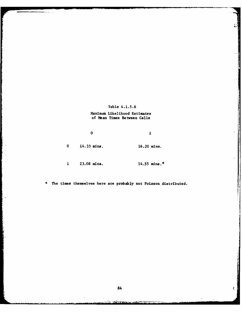
Table 4.1.5.6
Maximum Likelihood Estimatesof Mean Times Between Calls
0 1
0 14.33 mins. 16.20 mins.
1 23.08 mins. 14.55 mins.*
* The times themselves here are probably not Poisson distributed.
84 (

power outages over this period he concentrates his study on these two units.
The modelling process consists of a study of the available data for boiler
down times and running times, turbine down times and running times, a
combined model for the system's down time and a study of the system's
capability to meet the demand placed on the system. We will discuss only
a few aspects of the modelling of the boiler outage process.
After eliminating some obvious and explainable discrepencies in his
data, DeMarco was left with 1111 outage duration intervals and 774 running
duration intervals. A study of the outage duration intervals shows that such
intervals can be attributed to one of three types, say type a, b or c.
Running time is taken to be the length of time that the boiler system is
operating at the full capacity of 200 mw. Thus, while the system is
actually operating in some of the outage states (say, a, b), it is not up to
capacity and is considered to be in an "outage" state.
This system then can be in one of four states; running, outage a, outage
b, outage c. As the system operated every outage state was followed by a
return to the running state.
A lengthy and careful statistical analysis of the available data
indicated that the length of time the boiler was out depended only on the
outage state. Running times appeared to be a sequence of independent and
identically distributed random variables. However, if one considered only
the sequence of outage states, eliminating temporarily the intervening
running states, it appeared that this sequence was a Markov process. Thus,
one had the interesting result that if X = the state of the boiler at then
nth change of state (including the running state), {X was a second ordern
* 85

Markov process. That is {Xn I had transition probabilities of the form
PrIX+1 - JIX - i, X 1 = k).
Having to specifically account for this running state interuption to the
outage states is a nuisance. To eliminate the problem, DiMarco defines
three running states (call them 4, 5, 6) so that every outage of type a
returns the system to running state 4, every outage of type b returns the
system to running state 5, etc. In this way, the state process of the
boiler system is a Markov chain on E - {1,2,3,4,5,61. Thus, {Xn I on this
state space has one step transition probability matrix in the form:
0 0 0 1 0 0
0 o 0 0 1 0
0 0 0 0 0 1
P11 P1 2 P1 3 0 0 0
P21 P22 P2 3 0 0 0
P3 1 P32 P3 3 0 0 0
Having previously established that the lengths of the running times
and the lengths of the outage times are each sequences of independent
random variables and the several sequences are independent of each other,
one can now estimate the probability densities of these interval's lengths.
After a lengthy study of the data it was concluded that: these intervals
can all be fit by hyper-exponential distributions with a reasonable degree
of acceptability. The parameters of these hyper-exponentials are given
86
S -

Afl-A093 079 VIRGINIA POLYTECHN4IC INST AND STATE UNIV BLACKSBURG --ETC F/0 12/1A TUTORIAL ON NARKOV RENEWAL THEORY SEMD-REGENERATIVE PROCESES--ETC(U)DEC 60 R L DISNEY N0001177-C-07613
UNCLASSIFIED VTR-0-07 Nt
2 f f f f f f f f f f f f
I 2-8

I~~a ~ id ... . ..2. .
1401 111 2
111111-~
MIROOP RSLUINTS CHR

in the paper. They are of little concern to us here.
It is interesting to note, however, that the hyper-exponential density
function has a decreasing failure rate. This implies, for example, the
seemingly implausible condition that the longer the boiler goes without a
breakdown, the less likely it is to breakdown in the near future! DiMarco
argues that because of the complexity of these systems, it is unusual to
repair them correctly the first time. Therefore, for example, if the
boiler has been operational for a long period of time it is likely that it
was repaired correctly and therefore will continue to operate. If on the
other hand it was not repaired correctly (no matter how long it took to
repair it) then it is likely to fail shortly after coming out of repair.
In summary, then, the DiMarco model of the boiler portion of the steam
generators is a six state Markov renewal process whose requisite parameters
and distributions are estimated from the data. The model has an interesting
structure so that one has a degree of simplification and need not use the
full theory of Markov renewal process. That is, the model has the structure
Pr[X+l J,1 T I- T n _< tix i
= Pr[T+i - T < tJX i] Pr[X n+= JJX - i].
The sojourn times in state i do not appear to depend on the next state to be
visited as is possible in the full Markov renewal structure. (See formula
2.2.2 for a comparison.) This makes for a simplification in the analysis of
the model. But the hyper-exponential form of the running time and outage time
distributions (i.e., the Pr[Tn - Tn < t1Xn - il) still does not allow for a
87

model as simple as a continuous time Markov model. (i.e., these sojourn times
are not exponentially distributed.) A Markov model appears to be feasible
here but to develop it would require a more elaborate state space (probably
E x {1,2}, at least). Whether this elaboration would lead to a simpler
analysis than DiMarco gives to the Markov renewal model is a moot point.
4.1.7. Other Applications. There are many other applications that have
been made of Markov renewal process thoery. We can briefly mention a few here.
The reader is invited to consult the noted literature for details.
4.1.7.1. The Daganzo (1975) Study. Road traffic has long been an area of
application for random process theory. We briefly mentioned a study
of road traffic as a Markov renewal process whose states were identified with
leaders and followers in section.
Daganzo used a three state Markov renewal process to study the behavior of
traffic on a two lane road. However, he identifies these states with fast
moving vehicles and slow moving vehicles. In this way he obtains three states
identified with fast moving vehicles that are moving fast (i.e., unimpeded in
a platoon) slow moving vehicles (alone or in a platoon) and fast moving
vehicles moving slowly (i.e., impeded in a platoon).
His study concentrates on the formation and dissipation of platoons of
traffic, passing characteristics, road capacity and the other usual measures
of road traffic. Of particular interest in the study is the assumption that
vehicles have physical dimensions (most previous studies assumed vehicles
were points in a point process). For this reason one can have (and Daganzo
studies) the formation of platoons not only by fast vehicles catching up
88

with slow vehilles but by one platoon extending so as to encounter another
platoon. In this way, the author can examine road traffic in medium and
heavy traffic - a study rather different from older models of vehicles as
points, light traffic conditions, platoons that do not interact and leader -
follower models.
The author then observed vehicular flow on a two lane highway and collected
data on 295 vehicles to estimate the parameters of his model. He also col-
lected data on 476 other vehicles to test the predictive value of his finished
model. The results of this part of the analysis show that this Markov renewal
model of road traffic is superior to the then existing models. Indeed, this
model is shown to be a generalization of two other existing models so that by
particularizing the parameters of the model one can obtain other, previously
developed models which seem to be adequate for light traffic conditions but
inadequate for moderate to heavy traffic.
Furthermore, the Daganzo model seemed to fare better than some other models
which are also Markov renewal models but on different state spaces. The author
concludes that his model, while still in need to improvement, seems to produce
more realistic results than models that existed at the time.
4.1.7.2. The Lee (1979) Study. The study of fatigue has been an ongoing
enterprise in industrial engineering almost since the time of Taylor. In a
recently completed study, Lee attempts to build a stochastic model of the
physiologic processes that produce fatigue and to study the interaction of
fatigue inducing work and lengths of rest periods. His model, which attempts
to include many of the results found by many empirical studies, is much too
detailed to summarize here. The reader interested in the application of Markov
* 89

renewal theory to a classical problem in industrial engineering is invited to
consult this important study. To the best of our knowledge this study is
about the first to attempt a modelling of the underlying physiologic processes.
Most previous studies had been statistical and empirical.
4.2. Other Studies. In an unpublished thesis, Sim (1976) briefly reviews
the theory of Markov renewal processes and then provides an annotated
bibliography of applications of the theory to studies such as queues and
Geiger counters as well as to "real-life" applications. We simply list here
the areas where the applications have appeared. The Sim thesis should be
consulted for precise references and source documents.
a. Movement of Coronary Patients in a Hospital.
b. Clinical Trials with Acute Leukemia Patients.
c. Screening for Chronic Disease (with applications to cancer).
d. Human Reproduction.
e. Description of Sleep Patterns.
f. Behavior Sequences.
g. Social Mobility.
h. Time Shared Computer Models.
It is interesting to note in this listing that the use of a Markov renewal
model seems to be prevalent in the social and biological sciences. We have
not noticed the same incursion in engineering and operations research.
A few other applications (items [161-[21] in the bibliography) have
come to our attention. We would be interested in obtaining references to
other applications not noted in the references in our bibliography.
90

V. SUMMARY AND AFTERWORD
5.0. Summary. In the brief space available to us, but really because I lost
enthusiasm for saying more, we have tried to accomplish two things. First we
have tried to present an encapsulated version of some of the main ideas of
Markov renewal theory. That version is neither a primer nor a treatise on the
topic. Second we have tried to expose some of the areas of application of this
theory. In those discussions we have kept the manipulations to a minimum so as
to expose the ideas rather than dazzle the audience with our erring ability to
use mathematics. Thus, for example, we assumed that hiding places in a terrain
were distributed as a Poisson process in example 4.1.1. Clearly, that is a
silly assumption. But our interest was not to avoid silliness as much as to
show that Markov renewal theory had been applied and how.
In section IV we tried to expose some of the areas where the theory
developed in sections II and III had been applied. Most of these applications
have been "real life" in the sense that the researchers built a Markov renewal
model based on some existing phenomena, used data collected on the system to
estimate parameters of the model, exercised the model to obtain information
about the phenomena and used this information to recommend policy, predict
outcomes or gain new insights into previously little understood phenomena.
In the appropriate cases, it appeared that models built on Harkov renewal
process theory were more appropriate than models based on the more often
used methods of renewal theory or Markov process theory. That is, we think
we have demonstrated that such models are useful to a host of modelling
activities.
91
5.1. Afterword. The theory of Harkov renewal processes is nearly complete.
Literature on the topic is, as is most applied probability, spread over the
relevant journals of the world. There is no one home for the topic. Material
on the topic is beginning to reach the textbooks though it has been in the
research literature for over 20 years. Applications of the theory to topics
such as queueing and reliability have been going on for nearly 20 years, not
always recognized as such. Indeed, there is reason to believe that the
applications to queueing have driven queueing into new areas. Conversely,
queueing problems have provided an impetus for the further development of the
theory of Markov renewal processes. Modern queueing theory is a much different
animal than that exposed in most currently available textbooks.
There is still much to be done at the theory-application interface. We
have seen that the computation of most quantities of interest rely on the
Markov renewal function. Except for special structure on the semi-Harkov
kernel, this function is difficult to compute. (Of course, if one only wants
steady state behavior, this function need not be computed.) Whether one can
develop efficient computational algorithms to help in these computations or
can develop a theory of approximations is an open question. Research work at
present is pursuing both of these topics.
Statistical properties of the processes are discussed and sumarized in
the Sim paper. There is a need to extend, unify and make available to
potential users this knowledge.
Finally, we need more experience in the use of these topics for real life
modelling. In those cases where they have been used for models they seem to
perform well. But there are potential areas of application where they have
92 0

Ii
not been used and areas where they have been used but are still inadequate
for modelling the processes.
93

Bibliography
The first 9 references here are basic to the theory of Harkov renewal
processes or present some aspect of the topic referenced in the notes. The
list is far from complete. Reference [1] is a good elementary introduction
to the topic for those whose background includes a study of Markov processes
and renewal theory. Reference [2] is a textbook that includes a lengthy
discussion of all of these topics and much more.
[1] ginlar, E. (1975), "Markov Renewal Theory", Mgmt. Sci., 21, 727-752.
A nice discussion of Harkov renewal processes on finite state spaces.
The references provide the reader with an introduction into the mathematical
literature of the topic and several applications and examples not included
in our bibliography.
(21 ginlar, E (1975), Introduction to Stochastic Processes, Prentice-Hall,
Englewood Cliffs, N.J.
Chapter 10 of the book is one of the few textbook discussions of Harkov
renewal processes. The book provides proofs of most of our assertions as well
as additional examples. The book is non-measure theoretic and is suitable
for a first graduate text in random processes for operations researchers.
[3] Disney, R. L., Farrell, R. L., and de Morais, P. R. (1973), "ACharacterization of M/G/I/N Queues with Renewal DepartureProcesses", Mgmt. Sci., 19, 1222-1228.
A rather complete discussion of departure processes from M/G/l/N(N_<-)
queues. The process is shown to be a Markov renewal process. It is shown
that in 4 special cases (and only those 4 cases) this Markov renewal process
has {Tn+ I - Tn) as a sequence of i.i.d. random variables.
[4] Disney, R. L. and de Morais, P. R. (1976), "Covariance Properties of theDeparture Process of M/Ek/l/N Queues", Transactions (A.I.I.E.), 8,169-175.
A thorough study of the indicated covariances of lag 1 including graphical
results of some of these. The bibliography includes most of the work done on
the problem up to about 1970.
9494

[5] Fabens, A. J. (1961), "The Solution of Queueing and Inventory Models bySemi-Markov Processes", J. Roy. Stat. Soc., Ser. B., 23, 113-127,(with a correction note in same journal 25, 455-456.)
The first article that we know that explicitly uses Markov renewal
theory in the study of processes of interest to operations research.
[6] Finch, P. D. (1959), "The Output Process of the Queueing System M/G/l",
J. Roy. Stat. Soc., Ser. B., 21, 375-380.
An almost complete description of the departure process from M/G/1 queues.
The paper implicitly uses some properties of Markov renewal theory.
[7] Levy, P. (1954), "Processus semi-Markoviens", Proc. Int. Congr. Math.(Amsterdam), 3, 416-426.
[8] Pyke, R. (1961), "Markov Renewal Processes: Definitions and PreliminaryProperties (Part I)"; "Markov Renewal Processes with Finitely ManyStates (Part II)", Ann. Math. Stat., 32, 1231-1242 (Part I), 1243-1259 (Part II).
Along with [7] and [91 this is one of the pace setting articles. It
was "the" reference until rather recently.
[9] Smith, W. L. (1955), "Regenerative Stochastic Processes", Proc. Roy. Soc.London, Ser. A., 232, 6-31.
Along with [7] is "the" historically basic work in the field.
The following papers are dissertations. Hall was completed in the School
of Business Administration. Daganzo was completed in the Department of Civil
Engineering. The other two were completed in the Department of Industrial
and Operations Engineering. All 4 were done at the University of Michigan.
Some oi the work on these papers has appeared in journals. We are not aware
that there were any articles derived from these works that fully expose the
scope of the modelling activity. For that reason we note here the basic
dissertation rather than derived papers. We understand that copies are
available from University Microfilms International, 300 N. Zeeb Rd., Ann Arbor,
Michigan.
[10] Daganzo, C. (1975), Two Lane Road Traffic: A Stochastic Model, 136 pp.(incl. appendix and references).
[11] DiMarco, A. (1972), The Intermediate Term Security Assessment of a PowerGenerating System, 238 pp. (incl. appendix and references).
95

[12] Hall, W. K. (1969), A Queueing Theoretic Approach to the Allocation andDistribution of Ambulances in an Urban Area, 262 pp. (incl. appendixand references).
[13] Lee, M. W. (1979), A Stochastic Model of Muscle Fatigue in Frequent,Strenuous Work Cycles, 307 pp. (incl. appendix and references).
The following reference was supplied by Dr. Jeffrey Hunter, Dept. of
Mathematics, University of Auckland, Auckland, New Zealand. We understand
that copies can be obtained from him.
[14] Sire, D. A. (1976), Semi-Markov Processes and Their Applications, 158 pp.
(incl. references).
The following two papers were briefly referenced in the notes. However,
they contain several references not included above. Both were reasonably up
to date at time of their publication but much new work has appeared since
then. We are unaware of more current surveys of either the theory or
applications of Markov renewal processes.
115] Cheong, C. K., deSmit, J. H. A., and Teugels, J. L. "Notes on Semi-Markov Processes" (Part II: Bibliography), Discussion paper 7207,C.O.R.E., Universite Catholique de Louvain.
[16] Disney, R. L. (1975), "Random Flow in Queueing Networks: A Review andCritique", Transactions (A.I.I.E.), 7, 268-288.
We will not try to give a complete lising of queueing applications. The
following three entries are concerned with queueing applications.
[171 Cole, A. E., Jr. (1979) Airport Curbside Operations: A Queueing Modelwith Blocking, Doctoral dissertation submitted to the Department ofCivil Engineering, University of Michigan, Ann Arbor. 196 pp. (incl.appendix and references).
An interesting application of a multidimensional Markov process to study
a queue of vehicles at the curbside of airports. Data were collected and
analyzed at several major airports to validate the model. Readers might be
interested in the sampling methods used.
96 6

[181 Powers, J. E. and Lackey, R. T. (1975), "Interactions in Ecosystems:
A Queueing Approach to Modelling", Math. Biosci., 25, 81-90.
An interesting use of a queueing model to study a predator-prey
interaction.
[19] Purdue, P. (1975), "Stochastic Theory of Compartments: An Open, TwoCompartment, Reversible System with Independent Poisson Arrivals",Bull. Math. Biol., 37, 269-275.
One of several articles by this author on the use of queueing theory in
the study called "compartment models" in biology.
The following 2 papers are a bit off of the beaten path for operations
researchers. They do illustrate that the foregoing topics are not solely
in the domain of operations research.
[20] ginlar, E., Bazant, Z., and Osman, H. (1977), "Stochastic Processes forExtrapolating Concrete Creep", J. Engr. Mech. Div. of ASCE, 103,1069.-1088.
A very nice application of Markov renewal processes to a problem
describing some properties of creep in concrete.
[21] Rao, C. R. and Kshirsagar, A. M. (1978), "A Semi-Markovian Model forPredator-Prey Interactions", Biometrics, 34, 611-619.
97
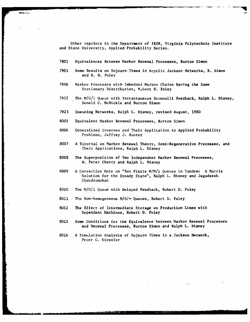
Other reprints in the Department of IEOR, Virginia Polytechnic Instituteand State University, Applied Probability Series.
7801 Equivalences Between Markov Renewal Processes, Burton Simon
7901 Some Results on Sojourn Times in Acyclic Jackson Networks, B. Simonand R. D. Foley
7906 Markov Processes with Imbedded Markov Chains Having the SameStationary Distribution, Robert D. Foley
7922 The M/G/1 Queue with Instantaneous Bernoulli Feedback, Ralph L. Disney,Donald C. McNickle and Burton Simon
7923 Queueing Networks, Ralph L. Disney, revised August, 1980
8001 Equivalent Markov Renewal Processes, Burton Simon
8006 Generalized Inverses and Their Application to Applied ProbabilityProblems, Jeffrey J. Hunter
8007 A Tutorial on Markov Renewal Theory, Semi-Regenerative Processes, andTheir Applications, Ralph L. Disney
8008 The Superposition of Two Independent Markov Renewal Processes,W. Peter Cherry and Ralph L. Disney
8009 A Correction Note on "Two Finite M/M/l Queues in Tandem: A MatrixSolution for the Steady State", Ralph L. Disney and JagadeeshChandramohan
8010 The M/G/l Queue with Delayed Feedback, Robert D. Foley
8011 The Non-homogeneous M/G/- Queues, Robert D. Foley
8012 The Effect of Intermediate Storage on Production Lines withDependent Machines, Robert D. Foley
8015 Some Conditions for the Equivalence between Markov Renewal Processesand Renewal Processes, Burton Simon and Ralph L. Disney
8016 A Simulation Analysis of Sojourn Times in a Jackson Network,Peter C. Kiessler

I


![Hidden Markov Model - Western Universitydlizotte/teaching/cs886_slides/MKarg_hmm_slides.pdf[5] L. Rabiner, A Tutorial on Hidden Markov Models and Selected Applications in Speech Recognition,](https://img.pdfslide.net/doc/110x75/5f0dc8747e708231d43c103e/hidden-markov-model-western-university-dlizotteteachingcs886slidesmkarghmm.jpg)