221B Lecture NotesQuantum Field Theory IV (Radiation Field)

1 Quantization of Radiation Field

Early development of quantum mechanics was led by the fact that electro-magnetic radiation was quantized: photons. Now that we have gone throughquantization of a classical field (Schrodinger field so far), we can proceed toquantize the Maxwell field. The basic idea is pretty much the same, exceptthat there are subtletites associated with the gauge invariance of the vectorpotential.

1.1 Classical Maxwell Field

The vector potential ~A and the scalar potential φ are combined in the four-vector potential

Aµ = (φ, ~A). (1)

Throughout the lecture notes, we use the convention that the metrix gµν =

diag(+1,−1,−1,−1) and hence Aµ = gµνAν = (φ,− ~A). The four-vector

coordinate is xµ = (ct, ~x), and correspondingly the four-vector derivative is

∂µ = (1c

∂∂t, ~∇). The field strength is defined as Fµν = ∂µAν − ∂νAµ, and

hence F0i = ∂0Ai − ∂iA0 = − ~A/c − ~∇φ = ~E, while Fij = ∂iAj − ∂jAi =

−~∇iAj + ~∇jA

i = −εijk ~Bk.In the unit we have been using where the Coulomb potential is QQ′/r

without a factor of 1/4πε0, the action for the Maxwell field is

S =∫dtd~x

[−1

8πF µνFµν − Aµj

µ]

=∫dtd~x

[1

8π

(~E2 − ~B2

)− Aµj

µ]. (2)

I included a possible source term for the Maxwell field (electric current den-sity) jµ = (ρ,~j/c). For a point particle of charge e, the charge density isρ = eδ(~x−~x0) while the current density is ~j = e~xδ(~x−~x0). They satisfy thecurrent conversation law

∂µjµ =

1

c

(∂

∂tρ+ ~∇ ·~j

)= 0. (3)

1

The gauge invariance of the Maxwell field is that the vector potentialAµ and Aµ + ∂µω (where ω is an arbitrary function of spacetime) give thesame field strength and hence the same action. Using this invariance, onecan always choose a particular gauge. For most purposes of non-relativisticsystems encountered in atomic, molecular, condensed matter, nuclear andastrophysics, Coulomb gauge is the convenient choice, while for highly rel-ativistic systems such as in high-energy physics. We use Coulomb gauge inthis lecture note:

~∇ · ~A = 0. (4)

A word of caution is that this gauge condition is not Lorentz-invariant, i.e.,the gauge condition is not frame independent. Therefore, when you go to adifferent frame of reference, you also need to perform a gauge transformationat the same time to preserve the Coulomb gauge condition. Another pointis that, in the Coulomb gauge, the Gauss’ law is

~∇ · ~E = 4πj0, (5)

where j0 is the charge density. Because ~E = − ~A − ~∇φ and the Coulombgauge condition, we find the Poisson equation

∆φ = −4πρ, (6)

and hence

φ(~x, t) =∫d~y

1

|~x− ~y|ρ(~y, t). (7)

Note that the potential is not retarded, but instantaneous (i.e., determinedby the charge distribution at the same instance).

Hamiltonian for a particle of electric charge e in the presence of theMaxwell field is

H =(~p− e

c~A)2

2m+ eφ. (8)

1.2 Quantization

In order to quantize the Maxwell field, we first determine the “canonicallyconjugate momentum” for the vector potential ~A. Following the definitionpi = ∂L/∂qi in particle mechanics, we define the canonically conjugate mo-mentum

πi =∂L∂Ai

= − 1

4πcEi =

1

4π

(1

c2Ai +

1

c~∇iφ

). (9)

2

In the absence of extrernal sources, the scalar potential identically vanishes inCoulomb gauge (see Eq. (7)). We drop it entirely in this section.1 Followingthe normal canonical commutation relation [qi, pj] = ihδij, we set up thecommutation relation

[Ai(~x), πj(~y)] = [Ai(~x),1

4πc2Aj(~y)] = ihδijδ(~x− ~y). (10)

To satisfy this commutation relation, we introduce the photon creation andannihilation operators

[ai(~p), aj†(~q)] = δijδ~p,~q, (11)

and expand the vector potential and its time derivative as

Ai(~x) =

√2πhc2

L3

∑~p

1√ωp

(ai(~p)ei~p·~x/h + ai†(~p)e−i~p·~x/h) (12)

Ai(~x) =

√2πhc2

L3

∑~p

(−i√ωp)(ai(~p)ei~p·~x/h − ai†(~p)e−i~p·~x/h). (13)

Here, ωp = Ep/h = c|~p|/h is the angular frequency for the photon. You cancheck that this momentum-mode expansion together with the commutationrelation Eq. (11) reproduces the canonical commutation relation Eq. (10) asfollows.

[Ai(~x), Aj(~y)]

=2πhc2

L3

∑~p,~q

(−i)[ai(~p)ei~p·~x/h + ai†(~p)e−i~p·~x/h, aj(~p)ei~q·~y/h − aj†(~q)e−i~q·~y/h]

=2πhc2

L3i∑~p

δij(ei~p·(~x−~y) + e−i~p·(~x−~y))

= 4πhc2iδ(~x− ~y). (14)

At the last step, we used the correspondence in the large volume limit∑

~p =L3∫d~p/(2πh)3.

The problem with what we have done so far is that we have not imposedthe Coulomb gauge condition Eq. (4) on the vector potential yet. Acting thedivergence on the momentum-mode expansion Eq. (12), we need

~p · ~a(~p) = 0. (15)

1Even when we have matter particles or fields, their charge density operator commuteswith the vector potential, and hence the discussion here goes through unmodified.

3

The meaning of this equation is obvious: there is no longitudinal photon.There are only two transverse polarizations. To satisfy this constraint whileretaining the simple commutation relations among creation and annihilationoperators, we introduce the polarization vectors. When ~p = (0, 0, p), the pos-itive helicity (right-handed) circular polarization has the polarization vector~ε+ = (1, i, 0)/

√2, while the negative helicity (left-handed) circular polariza-

tion is represented by the polarization vector ~ε− = (1,−i, 0)/√

2. In general,for the momentum vector ~p = p(sin θ cosφ, sin θ sinφ, cos θ), the circular po-larization vectors are given by

~ε±(~p) =1√2

(±~ε1 + i~ε2) , (16)

where the linear polarization vectors are given by

~ε1(~p) = (cos θ cosφ, cos θ sinφ,− sin θ), (17)

~ε2(~p) = (− sinφ, cosφ, 0). (18)

We can check that these two vectors give the complete orthonormal set bychecking

~ε∗λ(~p) · ~ελ′(~p) = δλ,λ′ , (19)∑λ

εiλ(~p)ε∗jλ (~p) = δij − pipj

~p2. (20)

These properties are satisfied for both the basis with linear polarizationsi, j = 1, 2 and the helicity basis i, j = ±. The last expression is a projectionon the transverse direction, consistent with the Coulomb gauge condition wehave imposed.

Given the polarization vectors, we re-expand the vector potential in termsof the creation/annihilation operators

Ai(~x) =

√2πhc2

L3

∑~p

1√ωp

∑±

(εi±(~p)a±(~p)ei~p·~x/h + εi±(~p)∗a†±(~p)e−i~p·~x/h) (21)

Ai(~x) =

√2πhc2

L3

∑~p

(−i√ωp)∑±

(εi±(~p)a±(~p)ei~p·~x/h − εi±(~p)∗a†±(~p)e−i~p·~x/h).

(22)

4

With this expansion, the Coulomb gauge condition is automatically satisfied,while the creation/annihilation operators obey the commutation relations

[aλ(~p), a†λ′(~q)] = δλ,λ′δ~p,~q (23)

for λ, λ′ = ±. We could also have used the linearly polarized photons

Ai(~x) =

√2πhc2

L3

∑~p

1√ωp

2∑λ=1

(εiλ(~p)aλ(~p)ei~p·~x/h + εiλ(~p)a

†λ(~p)e

−i~p·~x/h) (24)

Ai(~x) =

√2πhc2

L3

∑~p

(−i√ωp)2∑

λ=1

(εiλ(~p)aλ(~p)ei~p·~x/h − εiλ(~p)a

†λ(~p)e

−i~p·~x/h).

(25)

with[aλ(~p), a

†λ′(~q)] = δλ,λ′δ~p,~q (26)

for λ, λ′ = 1, 2. Clearly, two sets of operators are related by

a1 =1√2(a+ + a−), a2 =

i√2(a+ − a−). (27)

Once we have the mode expansion for the vector potential, one can workout the Hamiltonian

H =∫d~x

1

8π

(~E2 + ~B2

)=∑~p

∑±hωp

(a†±(~p)a±(~p) +

1

2

). (28)

Because hωp = c|~p|, the dispersion relation for the photon is the familiar oneE = c|~p| for a massless relativistic particle.

2 Classical Electromagnetic Field

Now that we found photons (particles) from the quantized radiation field,what is a classic electromagnetic field?

To answer this question, we study the quantum-mechanical Hamiltonianfor the photons in the presence of a source. Starting from the action Eq. (2),we find the Hamiltonian

H =∫d~x[

1

8π

(~E2 + ~B2

)− 1

c~A ·~j

]

5

=∑~p,λ

(hωpa

†λ(~p)aλ(~p)

−1

c

√2πhc2

L3

1√ωp

(~ελ(~p) ·~j(~p)aλ(~p) + ~ε∗λ(~p) ·~j∗(~p)a†λ(~p))

). (29)

Here, we omitted the zero-point energy because it is not relevant for thediscussions below, and the Fourier modes of the source is defined by

~j(~p) ≡∫d~x~j(~x)ei~p·~x/h, (30)

and ~j∗(~p) = ~j(−~p). The interesting point is that for each momentum ~p andpolarization state λ, the Hamiltonian Eq. (29) is of the type

hω(a†a− f ∗a− a†f), (31)

whose ground state is

hω(a†a− f ∗a− a†f)|f〉 = −hωf ∗f |f〉. (32)

In other words, the ground state of the Hamiltonian for photons in the pres-ence of a source term is a coherent state |f〉 ≡ ∏

~p,λ |fλ(~p)〉, with

fλ(~p) =

√2πh

L3

1

hω3/2p

~ε∗λ ·~j∗(~p). (33)

The vector potential has an expectation value in the coherent state, given by

〈f |Ai(~x)|f〉

=∑~p,λ

√2πhc2

L3

1

hω2p

(~εiλ(~p)fλ(~p)ei~p·~x/h + ~εi∗λ (~p)f ∗λ(~p)e−i~p·~x/h)

=2πh

L3

∑~p

c

hω2p

(jk∗(~p)ei~p·~x/h

∑λ

εiλ(~p)εk∗λ (~p) + c.c.

). (34)

Even though the expression is somewhat complicated, one can check thatthis expectation value satisfies

~∇× 〈f | ~B|f〉 = −∆〈f | ~A|f〉 =4π

c~j, (35)

6

using the identity Eq. (20) together with the Coulomb gauge condition ~∇· ~A =0. Actually, the term proportional to ~pi is a gradient −ih∇i and hence gauge-dependent. Ignoring the gauge-dependent term, we find a simpler expression

〈f |Ak(~x)|f〉 =2π

L3

∑~p

c

hω2p

(jk∗(~p)ei~p·~x/h + c.c.

)=

4π

c

1

L3

∑~p

(1

~k2jk∗(~p)ei~k·~x + c.c.

), (36)

which shows manifestly that it is a solution to the Poisson equation in thewave vector space ∆ = −~k2.

What we have learnt here is that the ground state for the photon Hamil-tonian in the presence of a source is given by a coherent state, which has anexpectation value for the vector potential. This expectation value is nothingbut what we normally obtain by solving Maxwell’s equations for the classicalMaxwell’s field.

The solution we obtained, however, is not a “radiation” because it doesnot propagate. We can produce a radiation by turning off the current instan-taneously at t = 0. Classically, it corresponds to a non-static source whichcan radiate electromagnetic wave. Quantum mechanically, we can use the“sudden” approximation that the same state given above now starts evolvingaccording to the free photon Hamiltonian without the source term from t = 0and on.

The time evolution of a coherent state is very simple. For the free Hamil-tonian H = hωa†a, the time evolution is

|f, t〉 = e−iHte−f∗f/2efa†|0〉

= e−f∗f/2e−iωa†at∞∑

n=0

fn

n!(a†)neiωa†ate−iωa†at|0〉

= e−f∗f/2∞∑

n=0

fn

n!

(e−iωa†ata†eiωa†at

)n|0〉

= e−f∗f/2∞∑

n=0

fn

n!(a†e−iωt)n|0〉

= e−f∗f/2efe−iωta†|0〉= |fe−iωt〉. (37)

In other words, the time evolution keeps a coherent state still a coherentstate, but with a different eigenvalue for the annihilation operator fe−iωt.

7

Then the expectation value for the vector potential can also be written downright away:

〈f, t|Ak(~x)|f, t〉 =4π

c

1

L3

∑~p

(1

~k2jk∗(~p)ei~k·~x−iωpt + c.c.

). (38)

One can see that this vector potential describes a propagating electromag-

netic wave in the vacuum because of the factor ei~p·~x/he−iωpt = ei(~k·~x−c|~k|t) with~k = ~p/h and ωp = c|~k|. The quantum mechanical state is still a coherentstate with time-dependent eigenvalues for the annihilation operators.

The analogy to Bose–Einstein condensate is intriguing. In the case ofBose–Einstein condensate, we have a collection of particles which can bedescribed either in terms of particle Hamiltonian or quantized Schrodingerfield. After the condensate develops, it cannot be described by the particleHamiltonian anymore, but rather by a “unquantized” version of Schrodingerfield. The system exhibits macroscopic coherence. For the case of an elec-tromagnetic wave, it is normally described by a classical Maxwell field. Butone can talk about photons which appear in quantized radiation field. Thenthe “unquantized” version of the Maxwell field exhibits the macrosopic co-herence.

Therefore, as long as the amplitude for the Maxwell field is “large,” thenumber–phase uncertainty relation can easily be satisfied while manifestingcoherence, and the quantum state is well described by a classical field, namelythe Maxwell field.

As an example, laser is described in terms of a coherent state of photons.The stimulated emission builds up photons in such a way that it becomes acoherent state.

3 Interaction With Matter

Now that we know how we get photons, we would like to discuss how photonsare emitted or absorbed by matter.

When I was taking quantum mechanics courses myself, I was very frus-trated. You hear about motivations why you need to study quantum me-chanics, and most (if not all) of the examples involve photons: Planck’s law,photoelectric effect, Compton scattering, emission spectrum from atoms, etc.But the standard quantum mechanics is incapable of dealing with creationand annihilation of particles, as we had discussed already. Now that we

8

have creation and annihilation operators for photons, we are in the positionto discuss emission and absorption of photons due to their interaction withmatter.

3.1 Hamiltonian

In this section, we deal with matter with conventional quantum mechanics,while with photons with quantized radiation field. This formulation is ap-propriate for decays of excited states of atoms, for instance. To be concrete,let us consider a hydrogen-like atom and its interaction with photons. Westart with the Hamiltonian

H =~p2

2m− Ze2

r. (39)

Obviously, this Hamiltonian does not contain photons nor their interactionwith the electron. The correct Hamiltonian for us is

H =(~p− e

c~A)2

2m− Ze2

r+∑~p,λ

hωpa†λ(~p)aλ(~p). (40)

The first term describes the interaction of the electron with the vector po-tential ~A(~x). For instance, the motion of electron in the constant magneticfield is described by this Hamiltonian with Ax = −By/2, Ay = Bx/2. Forour purpose, however, the vector potential is not a function of ~x alone, whichis an operator for the position of electron, but also contains creation andannihilation operators for photons. We rewrite the Hamiltonian Eq. (40 intwo pieces

H = H0 + V = He +Hγ + V, (41)

He =~p2

2m− Ze2

r, (42)

Hγ =∑~p,λ

hωpa†λ(~p)aλ(~p) (43)

V = −ec

~p · ~A+ ~A · ~p2m

+e2

c2

~A · ~A2m

. (44)

We regard H0 as the unperturbed Hamiltonian, and V as a perturbation.It is useful to know that ~p · ~A = ~A · ~p in the Coulomb gauge because thedifference is ~p · ~A− ~A · ~p = −ih~∇ · ~A = 0.

9

3.2 Free Hamiltonian

In perturbation theory, we have to solve the unperturbed system exactlyso that we can perturb around it. What are the eigenstates and energyeigenvalues of the unperturbed Hamitonian H0 in our case? The point hereis that there is no communication between the electron in He and photons inHγ. Therefore, all we need to know is the eigenstates and eigenvalues of twoseparate Hamiltonians. The full eigenstates are product of two eigenstates,and the eigenvalues sum of two eigenvalues. For instance, we can considerstates such as

|1s〉|0〉,|3d〉a†λ1

(~p1)a†λ2

(~p2)a†λ3

(~p3)a†λ4

(~p4)|0〉,|k, l,m〉aλ(~p)|0〉,

and so on. The first state with the ground state of the system, with electron inthe 1s state and no photons. The second state has the electron in an excited3d state, with four photons. The last state has the electron in the continuumstate with the momentum hk and angular momentum l,m together with aphoton. Their eigenvalues are simply the sum of the electron energy andphoton energy (energies).

Therefore, we have solved the unperturbed Hamiltonian H0 exactly.

3.3 Dipole Transition Rates

The next step is to deal with the interaction Hamiltonian V . What we useis the Fermi’s golden rule for transition rates

Wfi =1

h|〈f |V |i〉|22πδ(Ef − Ei) (45)

to the lowest order in perturbation theory.To be specific, let us consider the decay of 2p state to 1s by emission of

a photon. In other words,

|i〉 = |2p〉|0〉 (46)

|f〉 = |1s〉|~q, λ〉, (47)

where the one-photon state is defined by

|~q, λ〉 = a†λ(~q)|0〉. (48)

10

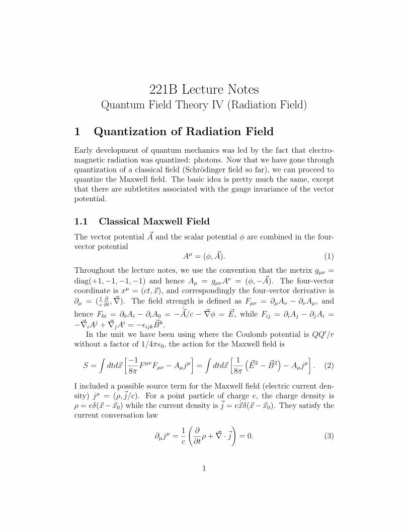
Because the initial and final states differ by one in the number of photons,and the vector potential ~A changes the number of photons by one, ~A2 termin V cannot contribute. Therefore,

〈f |V |i〉 = −ec

1

m〈f |~p · ~A(~x)|i〉, (49)

where we used the Coulomb gauge ~p · ~A = ~A · ~p. Now we can expand thevector potential in the momentum modes Eq. (21)

Ai(~x) =

√2πhc2

L3

∑~q′,λ′

1√ωq′

(εiλ′(~q′)aλ′(~q′)e

i~q′·~x/h + εiλ′(~q′)∗a†λ′(~q

′)e−i~q′·~x/h) (50)

with a word of caution. ~x is an operator describing the position of theelectron, while ~q′ is a dummy c-number variable you sum over (so is thehelicity λ′). ~p in Eq. (49), on the other hand, is also an operator describingthe momentum of the electron. Because the final state has a photon whilethe initial state doesn’t, only the piece with creation operator contributes tothe amplitude Eq. (49). Therefore,

〈f |V |i〉 = −ec

1

m〈~q, λ|

√2πhc2

L3

∑~q′,λ′

1√ωq′~ε∗λ′(~q

′)a†λ′(~q′)|0〉 · 〈1s|~pe−i~q′·~x/h|2p〉.

(51)The photon part of the matrix is element is easy:

〈~q, λ|a†λ′(~q′)|0〉 = δ~q,~q′δλ,λ′ (52)

and the summation over ~q′, λ′ goes away. (Note that we can also easily dealwith stimulated emission by having N photons in the initial state and N + 1photons in the final state, and the stimulated emission factor of

√N in the

amplitude comes out automatically.) Now the amplitude Eq. (51) reduces to

〈f |V |i〉 = −ec

1

m

√2πhc2

L3

1√ωq

~ε∗λ(~q) · 〈1s|~pe−i~q·~x/h|2p〉. (53)

Next, we point out that the exponential factor can be dropped as a goodapproximation. A higher order term in ~q · ~x/h is of order of magnitude ofthe size of the electron wave function a0 = h2/Zme2 = hc/αmc2 times the

11

energy of the photon Eγ = E2p − E1s = 12Z2α2mc2(1 − 1

22 ) divided by c,|~q| = Eγ/c, and is hence suppressed by a factor of Zα. This factor is smallfor a typical hydrogen-like atom. Finally, we use the identity

[He, ~x] = −ih ~pm, (54)

and hence

〈1s|~p|2p〉 = im

h〈1s|[He, ~x]|2p〉 = i

m

h(E1s−E2p)〈1s|~x|2p〉 = −im

hEγ〈1s|~x|2p〉.

(55)It is customary to write the last factor in terms of the electric dipole operator

~D = e~x, (56)

and hence the transition amplitude Eq. (53) is

〈f |V |i〉 =i

h|~q|√

2πhc2

L3

1√ωq

~ε∗λ(~q) · 〈1s| ~D|2p〉. (57)

Because the transition amplitude is given in terms of the matrix element ofthe electric dipole operator, it is called the dipole transition.

Back to Fermi’s golden rule Eq. (45), we now find

Wfi =1

h

1

h2~q2 2πhc2

L3

1

ωq

|~ε∗λ(~q) · 〈1s| ~D|2p〉|22πδ(Ef − Ei). (58)

When one is interested in the total decay rate of the 2p state, we sum over allpossible final states, namely the polarization and momentum of the photon.The decay rate of the 2p state is then

Wi =∑~q,λ

|~q|h2c

2πhc2

L3|~ε∗λ(~q) · 〈1s| ~D|2p〉|22πδ(Ef − Ei)

=∫ d~q

(2πh)3

2πc|~q|h

∑λ

|~ε∗λ(~q) · 〈1s| ~D|2p〉|22πδ(Ef − Ei). (59)

Here we used the large volume limit∑

~q = L3∫d~q/(2πh)3.

The transition matrix element of the electric dipole operator can be ob-tained easily. For example, for m = 0 state, only the z-component of the

12

dipole operator is non-vanishing because of the axial symmetry around thez-axis, and

〈1s| ~D|2p,m = 0〉 = e∫ ∞

0r2drdΩ

1

a32e−r/aY 0

0

√16

12

r

ae−r/2aY 0

1 r cos θ = e1√2

256

243a,

(60)with a = a0/Z. By taking the sum over the polarization states using the twolinear polarization states Eq. (17), only the first one contributes. Note alsothat 2πδ(Ef − Ei) = 2πδ(|~q| − (E2p − E1s)/c)/c and hence

Wi =∫ dΩq

(2πh)3|~q|2 (2π)2|~q|

h

∣∣∣∣∣εz,1(~q)e1√2

256

243a

∣∣∣∣∣2

=∫ dΩq

2πh4 |~q|3

(e

1√2

256

243a

)2

sin2 θ

=2

3

(256

243

)2

e2q3a2

h4

=256

6561Z4α5mc

2

h= 6.27× 108sec−1Z4. (61)

This result agrees well with the observed value of 6.2648×108 sec−1. In otherwords, the lifetime of the 2p state of hydrogen atom is W−1

i = 1.60×10−9 sec.It is interesting to think about sin θ behavior of the amplitude. The reason

behind it is fairly simple. Because we took m = 0 state as the initial state,there is no spin along the z-axis. On the other hand, in the final state, theatom does not carry spin (s-state) and the only carrier of spin is the photon.And the spin of the photon is always along the direction of its motion, eitherparallel (helicity +1) or anti-parallel (helicity −1). If the photon was emittedalong the z-axis, there is net spin along the positive z-axis in the final state,±1 for the helicity ±1 of the photon. To conserve angular momentum, suchan amplitude should vanish identically, which is done precisely by sin θ = 0 atθ = 0. Photon emission along the negative z-axis must be likewise forbidden,by sin θ = 0 at θ = π. The m = 0 state has its angular momentum l = 1oriented in the x-y plane, which matches the helicity of the photon whenemitted at θ = π/2, causing the maximum amplitude in sin θ = 1. Becausethe algebra is somewhat lengthy, albeit straightforward, it always helps tohave a simple understanding of the result based on intuitive arguments.

13

3.4 Photon Scattering on an Atom

The next process we will study is the scattering of a photon by an atom. Westart with the initial state of the atom A with a photon of momentum ~qi andpolarization λi (linear or circular). The final state is the atom in state Bwith a photon of momentum ~qf and polarization λf . When A = B, it is anelastic scattering, while when A 6= B, it is an inelastic scattering.

Because the initial and the final states have the same number of photons(one), the Fermi’s golden rule at the first-order in perturbation theory usedin the decay of 2p state discussed in the previous section cannot cause thisprocess. We have to go to the second order in perturbation theory. Therefore,we first develop the second-order formula of Fermi’s golden rule first, and thenapply it to the photon-atom scattering.

3.4.1 Second-order Fermi’s Golden Rule

We first recall the derivation of Fermi’s golden rule at the first order inperturbation theory. We use a derivation slightly different from that in theclass, but the result is the same. In class, we “turned on” the perturbationV at t = 0, and discussed the time evolution to t. In the end we obtainedthe result for t → ∞ limit. Here, we try to calculate the transition for aninfinite time interval from the beginning.

The time-dependent perturbation theory uses the interaction picture,where operators evolve according to the unperturbed Hamiltonian H0:

OI(t) = eiH0t/hOe−iH0t/h, (62)

while the states evolve according to the time-evolution operator

UI(tf , ti) = Te− i

h

∫ tfti

VI(t)dt(63)

from the infinite past. Here, V is the interaction Hamiltonian and VI(t) =eiH0t/hV e−iH0t/h. T stands for the time-ordered product of operators thatfollow it.

The initial and final states are eigenstates of the unperturbed Hamilto-nian, H0|i〉 = Ei|i〉, H0|f〉 = Ef |f〉. The amplitude we need is

limtf→∞

ti→−∞

〈f |UI(tf , ti)|i〉. (64)

14

Up to the first order, Taylor expansion of UI(tf , ti) gives

〈f |UI(tf , ti)|i〉 = 〈f |1− i

h

∫ tf

tiVI(t)dt|i〉+O(V 2). (65)

Rewriting VI(t′) = eiH0t′/hV e−iH0t′/h, and using the eigenvalues of H0 on the

initial and final states,

〈f |UI(tf , ti)|i〉 = δfi −i

h

∫ tf

tieiEf t/h〈f |V |i〉e−iEit/hdt+O(V 2). (66)

When ti → −∞ and tf →∞, the t integraion gives simply

limtf→∞

ti→−∞

〈f |UI(tf , ti)|i〉 = δfi −i

h2πhδ(Ef − Ei)〈f |V |i〉+O(V 2)

= δfi − i2πδ(Ef − Ei)〈f |V |i〉+O(V 2) (67)

The probability of the transition over the infinite time interval is then (as-suming f 6= i),

|〈f |UI(t)|i〉|2 = |〈f |V |i〉|2(2πδ(Ef − Ei))2. (68)

The squre of the delta function is of course singular. To see what it is, werewrite the square as

(2πδ(Ef − Ei))2 = 2πδ(Ef − Ei)

1

hlim

tf→∞ti→−∞

∫ ti

−tf

ei(Ef−Ei)t/hdt. (69)

Because the first delta function forces Ef = Ei in the integrand, the integralgives the (infinite) time interval T = tf − ti,

(2πδ(Ef − Ei))2 = 2πδ(Ef − Ei)

1

hT. (70)

Using this expression,

|〈f |UI(t)|i〉|2 = |〈f |V |i〉|22πδ(Ef − Ei)T

h. (71)

The probability of the transition per unit time, namely the transition rate,is therefore obtained from the above expression divided by the time intervalT ,

Wfi =1

h|〈f |V |i〉|22πδ(Ef − Ei). (72)

15

This is Fermi’s golden rule we had used at the first order in perturbationtheory.

Now we extend the discussion to the second order. The second-orderpiece in 〈f |UI(t)|i〉 is

1

2!

(−ih

)2

〈f |T (VI(t′)VI(t

′′)|i〉 = − 1

h2

∫ t

−∞dt′∫ t′

−∞dt′′〈f |VI(t

′)VI(t′′)|i〉. (73)

In the second expression, I used the explicit definition of time-ordering to-gether with the fact that two possible orderings give identical contributionscancelling the prefactor 1/2!. Using the definition of VI , and inserting thecomplete set of intermediate states 1 =

∑m |m〉〈m|, it becomes

= − 1

h2

∫ t

−∞dt′∫ t′

−∞dt′′〈f |VI(t

′)VI(t′′)|i〉

= − 1

h2

∫ t

−∞dt′∫ t′

−∞dt′′

∑m

eiEf t′/h〈f |V |m〉e−iEmt′/heiEmt′′/h〈m|V |i〉e−iEit′′/h

= − 1

h2

∫ t

−∞dt′∫ t′

−∞dt′′ei(Ef−Em)t′/hei(Em−Ei)t

′′/h∑m

〈f |V |m〉〈m|V |i〉. (74)

To integrate over t′′ from −∞, we have to worry about the convergence.One way to ensure the convergence is to add a small damping factor in theexponent eεt′′ that damps in t→ −∞, and the t′′ integral gives

= − 1

h2

∫ t

−∞dt′∫ t′

−∞dt′′ei(Ef−Em)t′/h hei(Em−Ei)t

′/h

i(Em − Ei) + ε

∑m

〈f |V |m〉〈m|V |i〉.

(75)Then the remaining t′ integral gives the delta function,

= − 1

h2 2πhδ(Ef − Ei)h

i(Em − Ei) + ε

∑m

〈f |V |m〉〈m|V |i〉

= −i∑m

〈f |V |m〉〈m|V |i〉Ei − Em + iε

2πδ(Ef − Ei). (76)

The ε appears in the same way as in the energy denominator in the Lippman–Schwinger equation. Putting together with the first-order piece, we find theamplitude

〈f |UI(t)|i〉 = δfi − i2πδ(Ef −Ei)

(〈f |V |i〉+

∑m

〈f |V |m〉〈m|V |i〉Ei − Em + iε

)+O(V 3).

(77)

16

3.4.2 Cross Section

The interaction Hamiltonian is the same as before,

V = −ec

~p · ~A(~x)

m+e2

c2

~A(~x) · ~A(~x)

2m. (78)

Here, Coulomb gauge is already used to simplify the first term. For thetransition amplitude

〈B; ~qf , λf |UI(tf , ti)|A; ~qi, λi〉, (79)

we have to keep the number of photons (from one to one). This can be done

by using the ~A · ~A operator in V at the first order, while using the ~p · ~Aoperator in V twice would also do the job. In terms of coupling factors, bothof these contributions appear at O(e2). Therefore,

〈B; ~qf , λf |UI(tf , ti)|A; ~qi, λi〉

= −i2πδ(Ef − Ei)

〈B; ~qf , λf |e2

c2

~A(~x) · ~A(~x)

2m|A; ~qi, λi〉

+∑m

〈B; ~qf , λf | − ec

~p· ~A(~x)m

|m〉〈m| − ec

~p· ~A(~x)m

|i〉Ei − Em + iε

(80)

up to the second order in e2.Let us start from the first term in the parentheses. Here, one factor of the

vector potential should annihilate the photon in the initial state, while theother should create the photon in the final state. That is done by taking thesquare of Eq. (21) and taking the cross term (with a factor of two of course),and picking the creation/annihilation operators of relevant momenta andpolarizations. We find

〈B; ~qf , λf |e2

c2

~A(~x) · ~A(~x)

2m|A; ~qi, λi〉

=e2

c21

m

2πhc2

L3

1√ωiωf

〈B; ~qf , λf |~εi · ~ε∗fa†λf

(~qf )e−i~qf ·~x/haλi

(~qi)ei~qi·~x/h|A; ~qi, λi〉

=e2

mc22πhc2

L3

1√ωiωf

~εi · ~ε∗f〈B|e−i~qf ·~x/hei~qi·~x/h|A〉. (81)

17

Here and below, we use the short-hand notation ~εi = ελi(~qi), and ~εf = ελf

(~qf ).Within the same spirit of approximation as in the dipole decay rate, we canignore ~q ·~x h for photon energies comparable to atomic levels, and we find

〈B; ~qf , λf |e2

c2

~A(~x) · ~A(~x)

2m|A; ~qi, λi〉 =

e2

mc22πhc2

L3

1√ωiωf

~εi · ~ε∗fδB,A. (82)

Now let us see what kind of intermediate states m contribute to the sumin Eq. (80). One possibility is that m is an atomic state I with no photon.2

Then we pick the relevant creation operator in the first matrix element andthe relevant annihilation operator in the second matrix element, and

∑I

〈B; ~qf , λf | − ec

~p· ~A(~x)m

|I〉〈I| − ec

~p· ~A(~x)m

|A; ~qi, λi〉Ei − Em + iε

=e2

c21

m2

2πhc2

L3

1√ωiωf∑

I

〈B; ~qf , λf |~p · ε∗fa†λf

(~qf )e−i~qf ·~x/h|I〉〈I|~p · εiaλi

(~qi)ei~qi·~x/h|A; ~qi, λi〉

Ei − Em + iε

=e2

c21

m2

2πhc2

L3

1√ωiωf

∑I

〈B|~p · ε∗fe−i~qf ·~x/h|I〉〈I|~p · εiei~qi·~x/h|A〉Ei − Em + iε

. (83)

Again for ~q · ~x h, it becomes

=e2

c21

m2

2πhc2

L3

1√ωiωf

∑I

〈B|~p · ε∗f |I〉〈I|~p · εi|A〉EA + hωi − EI + iε

. (84)

We used Ei = EA + hωi and Em = EI .The other possibility for the intermediate states in Eq. (80) is that m is an

atomic state together with two photons |m〉 = |I; ~qf , λf ; ~qi, λi〉. In this case,we pick annilation operator in the first matrix element and creation operatorin the second matrix element, and similar calculation as the previous casegives

∑I

〈B; ~qf , λf | − ec

~p· ~A(~x)m

|I; ~qf , λf ; ~qi, λi〉〈I; ~qf , λf ; ~qi, λi| − ec

~p· ~A(~x)m

|A; ~qi, λi〉Ei − Em + iε

=e2

c21

m2

2πhc2

L3

1√ωiωf

∑I

〈B|~p · εi|I〉〈I|~p · ε∗f |A〉EA − hωf − EI + iε

. (85)

2The state I may be either one of the bound atomic states or a continuum state.

18

We used Em = EI + hωf + hωi.Putting all of them together,

〈B; ~qf , λf |UI(tf , ti)|A; ~qi, λi〉

= −i2πδ(Ef − Ei)2πhc2

L3

e2

mc21

√ωiωf

(~εi · ~ε∗fδB,A

+1

m

∑I

〈B|~p · ε∗f |I〉〈I|~p · εi|A〉EA + hωi − EI + iε

+1

m

∑I

〈B|~p · εi|I〉〈I|~p · ε∗f |A〉EA − hωf − EI + iε

)(86)

The combination r0 ≡ e2/mc2 is called the classical radius of electron,3 andis numerically r0 = 2.82× 10−13 cm.

Finally, we obtain the expression for the scattering cross section. Wesquare the transition amplitude above to obtain the transition probability.We use Eq. (70) to deal with the square of the delta function, and devide theresult by the time interval T to obtain the transition rate:

Wfi = 2πδ(Ef − Ei)

(2πhc2

L3

)2

r20

1

ωiωf

∣∣∣∣∣~εi · ~ε∗fδB,A

+1

m

∑I

〈B|~p · ε∗f |I〉〈I|~p · εi|A〉EA + hωi − EI + iε

+1

m

∑I

〈B|~p · εi|I〉〈I|~p · ε∗f |A〉EA − hωf − EI + iε

∣∣∣∣∣2

. (87)

Total cross section is obtained by dividing the transition rate by the fluxof photons and summing over all possible final states. In our case, there isone photon in the initial state in the volume L3 moving with speed of light.Therefore, the photon meets the atom with a flux of one per area L2 per timeL/c, and hence the flux is c/L3. The summation over final states is done bysumming over final photon momentum ~qf and polarization λf . Using thelarge volume limit, we replace the sum over possible final moenta

∑~qf

by an

integral L3∫d~qf/(2πh)

3. Therefore,

σ =L3

c

∫ L3d~qf(2πh)3

∑λf

Wfi

= r20

c3

h2

1

ωiωf

∫d~qfδ(Ef − Ei)

∣∣∣∣∣~εi · ~ε∗fδB,A

3Lorentz tried to understand electron basically as a spherical ball spinning around.The electrostatic energy of a charged ball is approximately E ∼ e2/r, which he equated tothe rest energy of the electron mc2. That way, you can see the meaning of the “classicalradius of electron.”

19

+1

m

∑I

〈B|~p · ε∗f |I〉〈I|~p · εi|A〉EA + hωi − EI + iε

+1

m

∑I

〈B|~p · εi|I〉〈I|~p · ε∗f |A〉EA − hωf − EI + iε

∣∣∣∣∣2

= r20

ωf

ωi

∫dΩf

∣∣∣∣∣~εi · ~ε∗fδB,A

+1

m

∑I

〈B|~p · ε∗f |I〉〈I|~p · εi|A〉EA + hωi − EI + iε

+1

m

∑I

〈B|~p · εi|I〉〈I|~p · ε∗f |A〉EA − hωf − EI + iε

∣∣∣∣∣2

.(88)

The dependence on the size of the box disappeared as desired, and we didthe integration over |~qf | using the delta function δ(Ef −Ei) = δ(c|~qf |+EB−c|~qi| − EA).

3.4.3 Rayleigh Scattering

Rayleigh scattering is the photon-atom scattering in the regime where thephoton energy is much less than the excitation energy ∆E of the atom. Inthis case, the energy denominator is large and the cross section is suppressedas (hω/∆E)4. We will see this explicitly in the following calculation. Thesteep dependence on the cross section on the frequency (or wave length) ofthe photon is why the sky is blue and the sunset is red.

When hω ∆E, there are many cancellations in the amplitude. To seethis, we need to make each contribution to the amplitude look similar to eachother. Therefore, we rewrite the simple term ~εi · ~ε∗f in a form as ugly as therest. Then we can see the cancellations explicitly and obtain a form thatshows the suppression factor. We will assume A = B because the photondoes not have enough energy to excite the atom in the final state. It alsomeans ωi = ωf = ω.

The trick is the simple point

[~εi · ~x,~ε∗f · ~p] = ih~εi · ~ε∗f . (89)

Then the first term in the absolute square in Eq. (88) can be rewritten as

~εi · ~ε∗f =1

ih〈A|[~εi · ~x,~ε∗f · ~p]|A〉. (90)

Then we insert a complete set of states 1 =∑

I |I〉〈I|,

~εi · ~ε∗f =1

ih

∑I

(〈A|~εi · ~x|I〉〈I|~ε∗f · ~p|A〉 − 〈A|~ε∗f · ~p|I〉〈I|~εi · ~x|A〉

). (91)

20

Then we further use the same trick we used in dipole transitions backwards,

〈A|~εi · ~x|I〉 =1

EA − EI

〈A|[H0,~εi · ~x]|I〉 =−ihm

1

EA − EI

〈A|~εi · ~p|I〉. (92)

Therefore,

~εi · ~ε∗f = − 1

m

∑I

(〈A|~εi · ~p|I〉〈I|~ε∗f · ~p|A〉

EA − EI

−〈A|~ε∗f · ~p|I〉〈I|~εi · ~p|A〉

EI − EA

). (93)

This expression looks similar enough to the rest of the terms in Eq. (88).The cross section can then be written as

σ = r20

∫dΩf

∣∣∣∣∣− 1

m

∑I

(〈A|~εi · ~p|I〉〈I|~ε∗f · ~p|A〉

EA − EI

−〈A|~ε∗f · ~p|I〉〈I|~εi · ~p|A〉

EI − EA

)

+1

m

∑I

〈A|~p · ε∗f |I〉〈I|~p · εi|A〉EA + hω − EI + iε

+1

m

∑I

〈A|~p · εi|I〉〈I|~p · ε∗f |A〉EA − hω − EI + iε

∣∣∣∣∣2

= r20

1

m2

∫dΩf

∣∣∣∣∣−∑I

hω〈A|~p · ε∗f |I〉〈I|~p · εi|A〉(EA + hω − EI + iε)(EA − EI)

+∑I

hω〈A|~p · εi|I〉〈I|~p · ε∗f |A〉(EA − hω − EI + iε)(EA − EI)

∣∣∣∣∣2

. (94)

The terms in the absolute square are suppressed by hω.It turns out, however, that there is even further cancellation between two

terms. That is because

−∑I

〈A|~p · ε∗f |I〉〈I|~p · εi|A〉(EA − EI)2

+∑I

〈A|~p · εi|I〉〈I|~p · ε∗f |A〉(EA − EI)2

=m

ih

∑I

(−〈A|[~x · ε∗f , H0]|I〉〈I|[~x · εi, H0]|A〉

(EA − EI)2+〈A|[~x · εi, H0]|I〉〈I|[~x · ε∗f , H0]|A〉

(EA − EI)2

)

=m

ih

∑I

(〈A|~x · ε∗f |I〉〈I|~x · εi|A〉 − 〈A|~x · εi|I〉〈I|~x · ε∗f |A〉

)=

m

ih〈A|[~x · ε∗f , ~x · εi]|A〉 = 0. (95)

In the second last step, we used the completeness∑

I |I〉〈I| = 1. There-fore, we can subtract this vanishing expression inside the absolute square in

21

Eq. (94) and find

σ = r20

1

m2

∫dΩf∣∣∣∣∣−∑

I

(hω〈A|~p · ε∗f |I〉〈I|~p · εi|A〉

(EA + hω − EI + iε)(EA − EI)−hω〈A|~p · ε∗f |I〉〈I|~p · εi|A〉

(EA − EI)2

)

+∑I

(hω〈A|~p · εi|I〉〈I|~p · ε∗f |A〉

(EA − hω − EI + iε)(EA − EI)−hω〈A|~p · εi|I〉〈I|~p · ε∗f |A〉

(EA − EI)2

)∣∣∣∣∣2

= r20

1

m2

∫dΩf

∣∣∣∣∣∑I

(hω)2〈A|~p · ε∗f |I〉〈I|~p · εi|A〉(EA + hω − EI + iε)(EA − EI)2

+∑I

(hω)2〈A|~p · εi|I〉〈I|~p · ε∗f |A〉(EA − hω − EI + iε)(EA − EI)2

∣∣∣∣∣2

. (96)

This expression no longer has big cancellations, and shows that the crosssection is suppressed by (hω)4.

In order to make an order-of-magnitude estimate of the cross section, itis useful to rewrite the matrix element further using the same trick [~x,H0] =ih~p/m. We find

σ = r20m

2ω4∫dΩf

∣∣∣∣∣∑I

〈A|~x · ε∗f |I〉〈I|~x · εi|A〉EA + hω − EI + iε

+∑I

〈A|~x · εi|I〉〈I|~x · ε∗f |A〉EA − hω − EI + iε

∣∣∣∣∣2

. (97)

From this expression, the size of the matrix elements are of the order ofthe Bohr radius a = h2/Zme2, the energy denominator is of the order ofE2p−E1s = 3Z2e4m/8h2, and the classical radius of electron is r0 = e2/mc2 =2.82× 10−13 cm. Ignoring coefficients of order unity, we find

σ ∼ r20m

2ω4

((h2/Zme2)2

Z2e4m/h2

)2

= r20

(hω

Z2e4m/h2

)4

. (98)

Numerically, for Z ∼ 1 and λ ∼ 7000A (red), we have hω ∼ 0.28 eV, andσ ∼ 9.0×10−3 cm2. This is a very small cross section. For λ ∼ 4000A (blue),however, the cross section is (7/4)4 = 9.4 times larger. In a gas at STP, themean free paths are 4 × 108 km and 4 × 107 km, respectively. These arelong enough distances that Sun does not appear blurred by the atmosphere.

22

However, the scattered light by the atmospherer is 10 times stronger in bluethan in red, explaining why the sky is blue. Similarly, blue light is scatteredaway 10 times more in blue than in red when the Sun is setting and the lighttraverses a long distance in the atmosphere.

Note that it makes sense intuitively why the cross section vanishes forω → 0 or λ → ∞. For a photon with a long wave length, it is hard tosee any structure at scales less than λ. Therefore, the neutral atoms appearpoint-like neutral objects, and by definition, photon does not “see” them;it couples only to electric charges. Only for a sufficiently short wavelength,photon can see that the neutral atoms actually consist of electrically chargedobjects, and can scatter off them. Therefore, the cross section should vanishwith some power of 1/λ. With an actual calculation, we found that it goeswith the fourth power, a very steep dependence.

3.4.4 Resonant Scattering

In Eq. (88), it appears troublesome when EA + hω → EI . The energydenominator vanishes and the cross section blows up. What is wrong?

When you consider the scattering of a photon with hydrogen atom in the1s state, and when the photon energy is close to E2p − E1s, we can excitethe atom to the 2p state, which decays later down to 1s state again. Thiscauses a big enhancement in the photon-atom scattering crosss section. Wehad studied this phenomenon in the context of potential scattering before,and had identified such an enhancement as a consequence of a resonance. Wehad also learned back then that the energy of a resonance is slightly shifteddownward on the complex plane, namely the energy has a negative imaginarypart. How do we see that for the 2p state here?

The answer is quite simple. When you calculate a shift in the energyeigenvalue at the second order in perturbation theory, the formula is

∆E =∑f

〈i|V |f〉〈f |V |i〉Ei − Ef

. (99)

Here, i is the state of your interest (|2p〉 in our case) and f runs over allpossible intermediate states (|1s〉|~q, λ〉 in our case). However, when the in-termediate state is a continuum, Ei and Ef can in general be exactly thesame. That would cause a singularity. To avoid it, we take the same pre-scription as we took in Lippmann–Schwinger equation to insert a factor of

23

iε:

∆E =∑f

〈i|V |f〉〈f |V |i〉Ei − Ef + iε

. (100)

Having done that, we now write the denominator factor in the standard wayas

1

Ei − Ef + iε= P 1

Ei − Ef

− iπδ(Ei − Ef ). (101)

Therefore the energy shift now has an imaginary part! We find

=∆E = −π∑f

〈i|V |f〉〈f |V |i〉δ(Ei − Ef ). (102)

You can see that it is related to Fermi’s golden rule by

− Γi

2≡ =∆E = −1

2h∑f

Wfi = −1

2hWi, (103)

and hence the imaginary part of the energy is related to the decay rate of theunstable state (resonance) precisely in the way we discussed in the scatteringtheory.

In general, around hωi ∼ EI−EA, the cross section Eq. (88) is dominatedby one term,

σ = r20

ωf

ωi

∫dΩf

∣∣∣∣∣ 〈B|~p · ε∗f |I〉〈I|~p · εi|A〉

EA + hωi − EI + iΓI/2

∣∣∣∣∣2

, (104)

where ΓI is the width of the state I. The matrix elements vary slowly withωi, while the energy denominator produces a strong peak at hωi = EI −EA.The dependence is approximately that of Breit–Wigner function as we sawin the scattering theory. ΓI is the HWFM of the Breit–Wigner resonanceshape as a function of the energy, while τI ≡ 1/WI = h/ΓI is the lifetime ofthe resonance.

4 Multi-Pole Expansion

In many applications, it is useful to consider photons in angular-momentumeigenstates. This is equivalent to the multi-pole expansion of electromagneticfield.

24

4.1 Spinless Schrodinger Field

First of all, the multi-pole expansion of the Schrodinger field ψ(~x) withoutspin is given by the Laplace equation

(∆ + k2)ψ(~x) =

(1

r2

d

drr2 d

dr− l(l + 1)

r2+ k2

)ψ(~x) = 0. (105)

The solutions regular at the origin are

uklm(~x) = 2jl(kr)Yml (θ, φ). (106)

It is normalized as ∫d~xuklmu

∗k′l′m′ = δll′δmm′

2π

k2δ(k − k′). (107)

Expanding a field in terms of angular momentum eigenmodes is the multi-pole expansion:

ψ(~x) =∑lm

∫ dk

2πk2aklmuklm(~x). (108)

The canonical commutation relation [ψ(~x), ψ†(~y)] = δ(~x − ~y) implies thecommutation relation

[aklm, a†k′l′m′ ] = δll′δmm′

2π

k2δ(k − k′). (109)

This set of creation and annihilation operators obey delta-function normal-ization because we have not put the system in a box. Correspondingly, astate created by the creation operator also satisfies the delta-function nor-malization

〈k′l′m′|klm〉 = 〈0|ak′l′m′a†klm|0〉 = δll′δmm′2π

k2δ(k − k′). (110)

4.2 Vector Potential

How do we expand a vector potential? We certainly need to find vectors outof uklm. We do so by acting certain differential operators. Define

~uLkjm =

1

k~∇ukjm (111)

~uMkjm =

1√l(l + 1)

(~x× ~∇)ukjm (112)

~uEkjm =

1

k√l(l + 1)

~∇× (~x× ~∇)ukjm. (113)

25

Due to the reason we will see below, they are longitudinal, magnetic, and elec-tric multipoles, respectively. They all satisfy the Laplace equation Eq. (105)because the differential operators acting on ukjm all commute with the Lapla-cian. They also satisfy the normalization∫

d~x~uAkjm · ~uB∗

k′j′m′ = δABδll′δmm′2π

k22πδ(k − k′), (114)

for A,B = L,E,M . Given this orthonormal set, we expand the vectorpotential as

~A =∑lm

∑A

∫ dk

2πk2

√2πhc2

ω(aA

kjm~uAkjm + aA†

kjm~uA∗kjm), (115)

and correspondingly,

~A =∑lm

∑A

∫ dk

2πk2(−i)

√2πhc2ω(aA

kjm~uAkjm − aA†

kjm~uA∗kjm), (116)

The creation and annihilation operators satisfy the commutation relation

[aAkjm, a

A†kjm] = δABδll′δmm′

2π

k2δ(k − k′). (117)

You can check the commutation relation Eq. (10) with this multipole expan-sion.

In the Coulomb gauge, we simply drop A = L from the summation be-cause

~∇ · ~uLkjm =

1

k∆ukjm = −kukjm 6= 0, (118)

and hence does not satisfy the gauge condition. Electric and magnetic mul-tipoles satisfy the Coulomb gauge condition.

The reason behind the names is very simple. Electric (magnetic) multi-poles have non-vanishing radial component of electric (magnetic) field, while

magnetic (electric) multipoles don’t. Both ~uM,Ekjm describes a mode with total

angular momentum j, with parity (−1)j+1 for magnetic and (−1)j for elec-tric multipoles (we will see this in the next section). An important pointis that both multipoles vanish identically when j = 0, and hence a photoncarries always angular momentum j = 1 or more. This is easy to see. Themagnetic multipoles have basically the angular momentum operator acting

26

on the spinless case uMklm = (~x × ~∇)uklm = i

h~Luklm. Therefore it is non-

vanishing only when l 6= 0. The electric multipoles are curl of the magneticones, and again only non-vanishing ones are l 6= 0.

It may be confusing that I’m switching back and forth between j and l.Let us check what ~J = ~L+ ~S actually does on these modes. ~L = −ih(~x× ~∇)

is the usual one acting on the modes. (Note that we use ~L or ~p and theircommutation relations in this discussion, but we only use them as short-handnotation for differential operators. They are not operators acting on thephoton Fock space, but differential operators acting on the c-number modefunctions ~uA

klm with which we are expanding the operator vector potential.)The spin matrices are obviously those for spin one case, and are given by

Sx = −ih

0 0 00 0 10 −1 0

, Sy = −ih

0 0 −10 0 01 0 0

, Sz = −ih

0 1 0−1 0 00 0 0

.(119)

Note that ~uMkjm = i

h~Luklm. Acting ~J2 = ~L2 + 2~L · ~S + ~S2 on ~uM

kjm, we can see

that ~L2 = l(l + 1)h2, and ~S2 = 2h2 because ~L commutes with both of them.

The action of ~L · ~S needs to be worked out:

~L · ~S~uMkjm = −ih

0 Lz −Ly

−Lz 0 Lx

Ly −Lx 0

i

h

Lx

Ly

Lz

uklm

=

[Lz, Ly][Lx, Lz][Ly, Lx]

uklm

= −h2~uMkjm. (120)

Therefore ~L·~S = −h2, and hence ~J2 = ~L2+2~L·~S+~S2 = l(l+1)h2−2h2+2h2 =l(l + 1)h2. That is why uklm gives the total angular momentum j = l, andwe’ve used them interchangingly. It is also an eigenstate of the Jz = mh,because

Jz~uMkjm = (Lz + Sz)

i

h

Lx

Ly

Lz

uklm

=i

h

LzLx − ihLy

LzLy + ihLx

LzLz

uklm

27

=i

h

LxLz

LyLz

LzLz

uklm

= mh~uMkjm. (121)

It is not in a helicity eigenstate, however. The helicity is the spin along thedirection of the momentum h = (~S · ~p)/|~p|. If you act ~S · ~p on ~uM

klm, you find

(~S · ~p)~uMkjm = −ih

0 pz −py

−pz 0 px

py −px 0

Lx

Ly

Lz

uklm

= h2~∇× ~uMklm

= h2k~uEklm. (122)

The electric multipoles ~uEkjm also have the eigenvalues ~J2 = l(l + 1)h2, Jz =

mh. That can be shown by the fact that ~uEklm = (~S · ~p)~uM

kjm/h2k, and that

(~S · ~p) commutes with ~J . Acting (~S · ~p) on ~uEkjm brings back ~uM

kjm.

4.3 Parity

Parity is the reflection of space: ~x→ −~x. Another advantage of the multipoleexpansion is that the photon is not only in the angular momentum eigenstatebut also in the parity eigenstate. The combination of them leads to usefulselection rules in the transition amplitudes.

In quantum mechanics, parity P is a unitary and hermitean operator.Like any other symmetry operators such as translation, rotation, time evolu-tion, etc, it has to be unitary PP † = 1 to preserve the probabilities. But do-ing parity twice is the same as doing nothing, PP = 1. Then we find P = P †

and hence it is hermitean. Therefore, states can be classified according tothe eigenvalues of the parity operator. If the Hamiltonian is parity-invariant,PHP = H, it also means [P,H] = 0 (use P 2 = 1) and hence the parity isconserved. In other words, if the initial state is an eigenstate of the parity,and final state also should have the same parity eigenvalue. For instance, aparticle in a central potential is described by the Hamiltonian

H =~p2

2m+ V (r), (123)

28

which is parity invariant. To see this, we use the definition P~xP = −~x,and note that the canonical commutation relation [xi, pj] = ihδij requiresthe momentum to also flip its sign P~pP = −~p. The radius r = |~x| of coursedoesn’t change under parity. For convenience, I call the parity on the chargedparticle (say, electron) Pe instead of just P . This is because I need a separateparity acting on the vector potential below.

The parity on the vector potential is

Pγ~A(~x)Pγ = − ~A(−~x). (124)

Under this transformation, the electric and magnetic fields transform as

Pγ~E(~x)Pγ = − ~E(−~x), Pγ

~B(~x)Pγ = ~B(−~x). (125)

It is easy to check that the Hamitonian of the radiation field is invariantunder parity.

Finally, we look at the interaction Hamiltonian

(~p− ec~A(~x))2

2m. (126)

Acting Pe makes it to

Pe

(~p− ec~A(~x))2

2mPe =

(−~p− ec~A( ~−x))2

2m, (127)

which is not the same. But further acting Pγ makes it to

PγPe

(~p− ec~A(~x))2

2mPePγ = Pγ

(−~p− ec~A( ~−x))2

2mPγ =

(−~p+ ec~A(~x))2

2m=

(~p− ec~A(~x))2

2m(128)

and hence the Hamiltonian is invariant under the product P ≡ PγPe. There-fore the parity eigenvalue that is conserved is the product of parity eigenvaluesof electrons and photons.

Now we try to identify the parity of a photon in a multipole. The startingpoint is the property of the spherical harmonics

Y ml (π − θ, φ+ π) = (−1)lY m

l (θ, φ). (129)

The argument (π − θ, φ + π) corresponds to the reflected position vector−~x. Based on this property, it is usually said that the state with orbital

29

angular momentum l is an eigenstate of parity with the eigenvalue (−1)l.

The magnetic multipole mode function is defined by acting ~x× ~∇, which iseven under parity. Therefore,

~uMkjm(−~x) = (−1)j~uM

kjm(~x). (130)

The electric multiple mode functions are obtained by taking curl of the mag-netic ones, and therefore there is an additional sign under parity, and hence

~uEkjm(−~x) = (−1)j+1~uE

kjm(~x). (131)

Now the right-hand side of Eq. (124) is

− ~A(−~x) = −∑jm

∫ dk

2πk2(aE

jkm~uEjkm(−~x) + aM

jkm~uMjkm(−~x) + h.c.)

=∑jm

∫ dk

2πk2((−1)jaE

jkm~uEjkm(~x) + (−1)j+1aM

jkm~uMjkm(~x) + h.c.),(132)

where h.c. stands for hermitean conjugate. On the other hand, the onlyoperator in the multipole expansion of the vector potential is the creationand annihilation operators, and only they are affected by Pγ. The l.h.s ofeq. (124) is then

Pγ~A(~x)Pγ =

∑jm

∫ dk

2πk2(Pγa

EjkmPγ~u

Ejkm(~x)+Pγa

MjkmPγ~u

Mjkm(~x)+h.c.). (133)

Comparing Eqs. (133,132), we find

PγaEjkmPγ = (−1)jaE

jkm, PγaMjkmPγ = (−1)j+1aM

jkm. (134)

The parity eigenvalues of photon states in a given multipole are

Pγ|jkm,E〉 = PγaE†jkm|0〉 = (−1)jaE†

jkm|0〉 = (−1)j|jkm,E〉, (135)

where I used Pγ|0〉 = |0〉. Therefore the parity eigenvalue of a photon inelectric multipoles is given by Pγ = (−1)j. Similarly, they are Pγ = (−1)j+1

for photons in magnetic multipoles.Conservation of parity provides powerful selection rules in many systems,

especially atomic, molecular and nuclear transitions by emission or absorp-tion of photons. This is because electromagnetism conserves parity. Until

30

1957, all forces in Nature were believed to conserve parity. The space lookssymmetric between right and left, right? Of course! But in 1957, T.D. Leeand C.N. Yang pointed out that parity may be violated in weak interac-tions. Their study started with what was called τ -θ puzzle. These particleswere discovered in cosmic rays, later produced artificially in accelerators, andstudied (mostly) in bubble chambers. τ+ particle was identified by its decayinto π+ and π0 (remember Yukawa’s pions responsible for binding protonsand neutrons in nuclei), while θ+ into π+π+π−. Because pions have oddintrinsic parity, and the decay is dominated by S-wave, τ+ has even parityand θ+ odd. The puzzle was that they appeared to have exactly the samemass and lifetime. It was too much of a coincidence that Nature providestwo particles with identical mass and lifetime. Given this puzzle, Lee andYang pointed out that maybe τ+ and θ+ are not separate particles whichhappen to have the same masses and lifetimes, but are a single particle withdifferent decay modes. For this to be true, a particle must be decaying intofinal states with opposite parities, and hence the parity must be broken (i.e.,not conserved). Then they asked the question how well parity conservationhas been tested experimentally, and to surprise of many people, found thatthe parity conservation has been tested only in electromagetic and stronginteractions, to some extent in gravity, but never in weak interactions whichare responsible for nuclear β-decay and decay of τ and θ particles. They pro-posed various ways to test (or see violation of) parity in weak interactions.One of them was to study a possible correction between the spin of nucleusand the momentum of the β-electron. Under parity, spin remains the samewhile the momentum flips. Therefore, if there is any correlation between thespin and the momentum, it means parity is broken. This experiment wasdone soon after Lee–Yang’s paper by C.S. Wu. She studied the β decay of60Co. She was clever to use the then-novel discovery that one can polarizenuclei in a magnetic field even when the temperature is not so low. Recallthat the nuclear magneton is 2000 times smaller than the Bohr magneton,and it appears it would require an extremely large magnetic field and lowtemperature to polarize nuclei. However, a magnetic field polarizes unpairedelectrons in the atom, which in turn polarizes nuclei due to hyperfine inter-actions. This turned out to be a much more effective way to polarize nuclei.She still needed a cryostat of course. (I didn’t look up the parameters.) Shecould demonstrate that the β-electrons are emitted preferentially parallel tothe spin of the nucleus, while the preference slowly disappeared once sheturned off the cryostat. Since then, we know that there is a fundamental

31

distinction between left and right. The division in Congress has a deep root,indeed!

4.4 Multipole Transitions

Emission of photons in ~uE,Mkjm is called Ej or Mj transitions. For instance,

the electric dipole transition produces a photon in the state ~uEk1m, and is

called E1 transition. The coupling of a magnetic moment to magnetic fieldin the Hamiltonian can cause the emission of a photon by a M1 transition.Because jl(kr) = (kr)l/(2l + 1)!! at small r, higher multipole transitions aresuppressed by powers of kr, similarly to the reason why we could omit higherpowers in ~q · ~x/h in the 2p→ 1s E1 transition discussed above.

As an example, we recalculate the 2p to 1s transition using the multipoleexpansion. In this case, the angular momentum of the atom changes byone unit, which needs to be carried away by the photon. Therefore, onlypossibilities are E1 and M1 transitions. This way, you can see that the dipoletransitions are the only possibilities even before doing any calculations; thisis a big advantage in the multipole expansion. To proceed, we need the modefunctions uM,E for j = 1. We take |2p,m = 0〉 again as the initial state, andhence the only mode functions we need are ~uM,E

k10 . First,

~uMk10 =

i

h

Lx

Ly

Lz

2j1(kr)Y01

1√1(1 + 1)

=i

h

(L+ + L−)/2(L+ − L−)/2i

Lz

2j1(kr)Y01

1√2

= i

(Y 11 + Y −1

1 )/2(Y 1

1 − Y −11 )/2i

0

2j1(kr)1√2

=

√3

2π

sin θ sinφ− sin θ cosφ

0

j1(kr). (136)

Using the behavior for small kr, j1(kr) ' kr/3, we find

~uMk10 '

k√6π

y−x0

. (137)

32

On the other hand, the electric dipole mode is

~uEk10 =

1

k~∇× ~uM

k10 ' −√

2

3π

001

. (138)

Note that there is no suppression due to kr in the electric dipole mode andhence is dominant over the magnetic dipole transition. (Another reason whythe magnetic dipole transition is not important is because it is forbidden for2p→ 1s transition due to parity conservation. We actually know that beforeworking out the mode function.) In general, magnetic multipole transitionsare suppressed relative to the electric ones for the same multipole in non-relativistic systems.

The only important piece in the multipole expansion of the vector poten-tial is then

~A(~x) 3∫ ∞

0

dk

2πk2

√2πhc2

ωk

a†k10

−√

2

3π

0

01

. (139)

(I’m using a sloppy notation that 3 means the r.h.s. is only the importantpart of the l.h.s.) Then the interaction Hamiltonian is

V = −ec

1

mpzAz 3

e

mc

√2

3πpz

∫ ∞

0

dk

2πk2

√2πhc2

ωk

a†k10. (140)

The matrix element is (see Eq. (60))

〈1s|〈k10|V |0〉|2p,m = 0〉

=e

mc

√2

3π

∫ ∞

0

dk′

2πk′2√

2πhc2

ωk′〈k10|a†k′10|0〉〈1s|pz|2p,m = 0〉

=e

mc

√2

3π

√2πhc2

ωk

1√2

256

243am

hEγ. (141)

(Recall q = hk = Eγ/c = hωk/c.)The decay rate is again given by the Fermi’s golden rule Eq. (45). The

only non-trivial difference is that the summation over the final state is givenby ∑

f

=∑jm

∫ dk

2πk2, (142)

33

while only j = 1, m = 0 contributes in our case. Therefore,

Wi =1

h

∫ dk

2πk2 e2

m2c22

3π

2πh2c

q

(1√2

256

243a

)2m2

h2 (cq)22πδ(Ef − Ei)

=e2

h4 q3a2 2

3

(256

243

)2

, (143)

which precisely agrees with Eq. (61).As we have seen in this example, the advantage of the multipole expansion

is that the selection rule is manifest. For a given initial and final state withfixed angular momenta and parities, one can immediately tell that multipolewould dominate in the transition.

There is an example in nuclear γ decay from a 2+ state to a 5+ state.From the angular momentum consideration, the photon must be in the mul-tipoles of j = 3, 4, 5, 6, or 7. From the parity consideration, it has to haveeven parity. Therefore, allowed multipole transitions are M3, E4, M5, E6,M7. Higher multipoles have higher powers in kr and hence are suppressed.However, as we saw above, the electric multipoles have one less power inkr compared to the corresponding magnetic ones. Therefore, M3 and E4transitions appear with the same power in kr (third power) and they bothcontribute in this transition and they interfere.

5 Casimir Effect

So far, we had not cared much about the zero-point energy of the photonsin Eq. (28). It is often said that the zero-point energy just amounts to thebaseline energy and all other energies are measured relative to it. In otherwords, pretending it doesn’t exist is enough. But the zero-point energy playsa role if a change in the system affects the zero-point energy itself. (SeeMilonni, P. W., and Shih, M. L., 1992, Contemp. Phys. 33, 313. for areview.)

To be concrete, put two conducting plates parallel to each other. Thedistance between the plates is d (at z = 0 and z = d), and the plates arevery large of area L2 where we take L → ∞. To simplify the discussions,we also place thin plates at x = 0, x = L and y = 0, y = L to form abox. A conducting plate imposes boundary conditions on the radiation fieldE‖ = 0 and B⊥ = 0. Given these boundary conditions, the vector potential

34

is expanded in modes as

~A(~x) ∼ ~ε sin(nx, ny, nz)(πnx

Lx+

πny

Ly +

πnz

dz), (144)

for nx, ny, and nz non-negative integers. For each wave vector ~k = (πnx/L, πny/L, πnz/d),

the polarization vector is transverse: ~k · ~ε = 0. If one of the n’s vanishes,however, say ~k = (0, πny/L, πnz/d), the polarization vector ~ε = (1, 0, 0) isnot allowed because that would give Ax 6= 0 for any x (and generic y, z)and violates the boundary condition E‖ = 0. Therefore, we have only onepolarization whenever one of n’s vanishes.

The sum of zero point energies in this set up is therefore given by

U(d) =∑ ′1

2hω × 2 =

∑ ′

nx,ny ,nz

hc

[(πnx

L

)2

+(πny

L

)2

+(πnz

d

)2]1/2

. (145)

The summation∑ ′ means that whenever one of n’s vanishes, we drop the

multiplicity 2 for possible transverse polarizations. Because we regard thesize of the plate to be large L → ∞, we can replace the sum over nx, ny interms of integrals over kx,y = πnx,y/L,

U(d) =(L

π

)2∑ ′

nz

∫ ∞

0dkx

∫ ∞

0dkyhc

[k2

x + k2y +

(πnz

d

)2]1/2

. (146)

Recall that we are interested in the difference in the zero-point energywhen d is varied. Therefore, it is useful to compare it to the case when theplates don’t exist. We can compute the zero-point energy density in theinfinite volume as usual, and then calcualte the energy U0(d) multiplied bythe volume L2d:

U0(d) = Ld2∫ d~k

(2π)3hc[k2

x + k2y + k2

z

]1/2

= Ld2∫ ∞

0

dkx

π

∫ ∞

0

dky

π

∫ ∞

0

dkz

πhc[k2

x + k2y + k2

z

]1/2. (147)

What is observable is the difference

U(d)− U0(d)

=L2

π2hc∫ ∞

0dkxdky

∑ ′

nz

[k2

x + k2y +

(πnz

d

)2]1/2

− d

π

∫ ∞

0dkz

[k2

x + k2y + k2

z

]1/2

.(148)

35

Switching to the circular coordinates,∫ ∞

0dkxdky =

∫ ∞

0k⊥dk⊥

∫ π/2

0dφ =

π

4

∫ ∞

0dk2

⊥,

we find

U(d)− U0(d)

=L2

π2hcπ

4

∫ ∞

0dk2

⊥

∑ ′

nz

[k2⊥ +

(πnz

d

)2]1/2

− d

π

∫ ∞

0dkz

[k2⊥ + k2

z

]1/2

.(149)

This expression appears problematic because it looks badly divergent. Thedivergence appears when the wave vector is large, which corresponds to highfrequency photons. The point is that the conducting plates are transparentto, say, gamma rays, or in general for photons whose wavelengths are shorterthan interatomic separation a. Therefore, there is naturally a damping factorf(ω) = f(c(k2

⊥ + k2z)

1/2) with f(0) = 1 which smoothly cuts off the integralfor ω >∼ c/a. In particular, f(∞) = 0. Then the expression is safe and allowsus to use standard mathematical tricks. Changing to dimensionless variablesu = (k⊥d/π)2 and nz = kzd/π,

U(d)− U0(d) =π2L2hc

4d3

∫ ∞

0du

∑ ′

nz

√u+ n2

z −∫ ∞

0dnz

√u+ n2

z

f(ω).

(150)Interchanging the sum and integral, we define the integral

F (n) =∫ ∞

0du√u+ n2f(ω) =

∫ ∞

n2du√uf(ω) (151)

with ω = πc√u/d in the last expression. Using this definition, we can write

U(d)− U0(d) =π2L2hc

4d3

1

2F (0) +

∞∑n=1

F (n)−∫ ∞

0dnF (n)

. (152)

Here we can use the Euler–McLaurin formula

1

2F (0) +

∞∑n=1

F (n)−∫ ∞

0F (n) = − 1

2!B2F

′(0)− 1

4!B4F

′′′(0)− · · · . (153)

36

The coefficientss Bk are Bernouilli numbers defined by the Taylor expansion

x

ex − 1=

∞∑k=0

Bkxk

k!, (154)

and B0 = 1, B1 = −1/2, B2 = 1/6, B4 = −1/30, and all odd ones B2n−1

vanish except B1.Here is a physicist’s proof of the Euler–McLaurin formula. Using the Taylor expansion

that defines the Bernouilli numbers, we replace x to a derivative operator ∂x

∂x

e∂x − 1=∞∑

k=0

Bk∂k

x

k!. (155)

We act this operator on a function F (x) and integrate it over x from 0 to ∞,∫ ∞0

dx∂x

e∂x − 1F (x) =

∫ ∞0

dx∞∑

k=0

Bk∂k

x

k!F (x). (156)

The l.h.s. of Eq. (156) is then∫ ∞0

∞∑k=0

Bk∂k

x

k!F (x) =

∫ ∞0

F (x)dx +∞∑

k=1

Bk

[∂k−1

x

k!F (x)

]∞0

=∫ ∞

0

F (x)dx−∞∑

k=0

Bk1k!

F (k−1)(0)

=∫ ∞

0

F (x)dx +12F (0)−

∞∑k=1

B2k1

(2k)!F (2k−1)(0). (157)

On the other hand, the r.h.s. of Eq. (156) is∫ ∞0

dx∂x

e∂x − 1F (x). (158)

By Taylor expanding the denominator,

∂x

e∂x − 1F (x) = −

∞∑n=0

∂xen∂xF (x). (159)

Note that ea∂xF (x) =∑∞

m=01

m!amF (m)(0) = F (x + a) and hence the r.h.s. is∫ ∞

0

dx∂x

e∂x − 1F (x) = −

∫ ∞0

dx∂x

∞∑n=0

F (x + n) =∞∑

n=0

F (n). (160)

By comparing both sides of Eq. (156), we now find∞∑

n=0

F (n) =∫ ∞

0

F (x)dx +12F (0)−

∞∑k=1

B2k1

(2k)!F (2k−1)(0). (161)

37

Moving first two terms in the r.h.s. to the l.h.s, we obtain the Euler–McLaurin formula

12F (0) +

∞∑n=1

F (n)−∫ ∞

0

F (x)dx = −∞∑

k=1

B2k1

(2k)!F (2k−1)(0). (162)

Wondering why all odd Bk vanish except for B1? It is easy to check that

x

ex − 1+

12x =

x(2 + ex − 1)2(ex − 1)

=x

2coth

x

2(163)

which is manifestly an even function of x.Going back to the definition of our function F (n) Eq. (151), we find

F ′(n) = −2n2f(πcn/d). (164)

As we will see below, we have d of order micron in our mind. This distanceis far larger than the interatomic spacing, and hence f(πcn/d) is constantf = 1 in the region of our interest. Therefore, we can ignore derivativesf (n)(0), and hence the only important term in the Euler–McLaurin formulaEq. (153) is F ′′′(0) = −4. We obtain

U(d)− U0(d) = −π2L2hc

4d3F ′′′(0)

1

4!B4 = −π

2L2hc

720d3. (165)

In other words, there is an attractive force between two conducting plates

F = [U(d)− U0(d)]′ =

π2L2hc

240d4(166)

which is numerically0.013dyn/cm2

(d/µm)3(167)

per unit area. This is indeed a tiny force, but Sparnay has observed itfor the first time in 1958. He placed chromium steel and aluminum platesat distances between 0.3–2µm, attached to a spring. The plates are alsoconnected to a capacitor. By measuring the capacitance, he could determinethe distance, while the known sping constant can convert it to the force.

38