226 recruiting suppliers for reverse production systems.doc) - Optimization … · · 2007-03-14Recruiting Suppliers for Reverse Production Systems: an MDP Heuristics Approach Wuthichai

1

Recruiting Suppliers for Reverse Production Systems: an MDP Heuristics Approach Wuthichai Wongthatsanekorn1, Matthew J. Realff2, Jane C. Ammons1

1Georgia Institute of Technology School of Industrial and Systems Engineering Atlanta, GA 30332-0205 2Georgia Institute of Technology School of Chemical and Biomolecular Engineering Atlanta, GA 30332-0100 Corresponding Author: Wuthichai Wongthatsanekorn School of Industrial and Systems Engineering Georgia Institute of Technology Atlanta, GA 30332 Email: [email protected] Phone: 404-894-7792

Abstract In order to achieve stable and sustainable systems for recycling post-consumer goods, frequently it is necessary to concentrate the flows from many collection points of suppliers to meet the volume requirements for the recycler. The collection network must be grown over time to maximize the collection volume while keeping costs as low as possible. This paper addresses a complex and interconnected set of decisions that guide the investment in recruiting effort. Posed as a stochastic dynamic programming problem, the recruitment model captures the decisions for the processor who is responsible for recruiting material sources to the network. A key feature of the model is the behavior of the collector, whose willingness to join the network is modeled as a Markov process. An exact method and two heuristics are developed to solve this problem, then their performance is compared in solving practically sized problems. Key words Recruiting, Reverse Production System, MDP Heuristics

1. Introduction The paper addresses on the concentration of post-consumer material flows through the

interaction between suppliers (agents) and a processor (recruiter). In forward supply chains, one processor negotiates with many suppliers in order to acquire the required resources for production to meet the demand. The processor has the ability to control the amount of material from the suppliers. The main uncertainty is usually the demand in the market. In reverse supply chains, the return flows from the consumers are a significant uncertainty. The reverse system consists of the activities such as collection, cleaning, disassembly, testing, and sorting, storage, and recovery operations. This paper focuses on the collection segment where the recycling processor attempts to retrieve used materials from various sources under uncertainty.

2

In order to build a successful collection network, we consider the problem of recruiting suppliers. In this case “suppliers” are typically local aggregators of material who work with consumers or very localized material handlers, such as supermarkets, to produce a regular supply of material. Careful planning of the supply network to support the recycling plant can be critical factor in the success or failure of the production operations. The interaction in the recruitment process is between business-to-business (B2B) entities rather than business-to-customer (B2C). This makes the process more complicated because both parties have power to negotiate.

In a reverse supply chain, planning the collection network to supply the capital intensive processing plant can be a crucial factor in the success or failure of recycling operations. For example, in the past decade, two major carpet recycling companies (Evergreen Nylon Recycling and PA2000) suffered major financial problems that led to the closure of the recycling plants. One explanation is the high cost of the supply materials resulting from widely dispersed collection points. Hence, the objective is to provide the collection capacity at low enough cost to make it viable. However, the processor is faced with a significant challenge. Processors are typically not familiar with the waste business; the collection of “trash” is not a core competency of their organization, nor do they have existing waste hauling contracts that they can exploit to get the material. Often, they do not have vertical integration to the retail sector and hence do not control the point of contact with the customers. This leads to the need to recruit a layer of suppliers to the system. In the case of recycled carpet this might be the retailers who sell carpet, as they are the ones to whom used carpet may be returned by the installers. According to the data from Carpet America Recovery Effort’s Annual Report in 2004, 4,000 million pounds of used carpet is discarded to the landfill in year 2003 while less than 100 million pounds was recycled. This number is growing rapidly as raw material costs rise. However, the carpet industry has had limited success with large scale recycling of nylon carpets despite the financial potential. Post consumer carpet scrap is priced at approximately $0.06 a pound

1 for truck load quantity

(40,000 pounds or more) while nylon 6 (after processing nylon-6 scrap) is priced at $1.592

for truck load quantity. One solution to this recruitment problem is to subcontract the responsibility of recruiting

suppliers to a local regional collector. The collector is then allocated a budget with which to recruit the retailers to the network, which could include financial incentives. Alternatively, the processor may decide to perform the recruitment and collection itself, and the budget would most likely reflect the amount of time and personnel resources that are devoted to a particular region.

Recruitment models in the literature focus on employment recruitment, human resource management, and physiological models in medical research (Darmon 2003, Treven 2006, Hawkins 1992, Georgiou and Tsantas (2002). Mehlmann (1980) use a recruitment concept for a long-term manpower planning problem. Coughlan and Grayson (1998) examine the problem where the individual distributors play two key roles in network marketing organizations (e.g. Amway, Mary Kay and NuSkin): they sell product, and they recruit new distributors. They develop a model of network marketing organization network growth that shows how compensation and other network characteristics affect growth and profitability of the distributor. In their context, one distributor recruits others by socially interacting with them in one form or another. They represented this process by adapting a diffusion model formulation to the recruitment process (Bass 1969). This model allows for network growth 1

Canada's Waste Recycling Marketplace (2006) 2

IDES The Plastics Web (2006)

3

via both inherent attraction (the innovation effect) and the spread of word-of-mouth (the imitation effect). They introduce a recruitment function which includes innovation and imitation terms. This paper explores the notion of the recruitment of the collectors, instead of the distributors. Furthermore, the recruitment process is represented in a more complex form, not just a closed-form function.

The recruitment model which is posed as a stochastic dynamic programming problem has some similarities to the Restless Bandits Problem, first introduced by Whittle (1988). The continuous-time version of the problem with a time-average reward criterion was developed in a dynamic programming framework. He then introduced a relaxed version of the problem, which can be solved optimally in polynomial time. More literature review in this area is discussed at the end of section 3.

The paper is organized as follows. In section 2, we more formally define the problem. The modeling of the problem is discussed in section 3. In section 4, we present three methods to solve the problem. In section 5, we describe the computational experiments that illustrate efficiency of our algorithms. Finally, in section 6, we develop some conclusions and ideas for future research.

2. Problem Definition and Modeling We refer to the problem of recruiting suppliers in a reverse production system as the

recruitment problem. Recruitment is a negotiating process that involves two parties: processor and supplier. We denote a supplier as an agent throughout the paper and a processor as a recruiter. The recruiter cannot retrieve material from the agent unless both parties agree to it through the recruitment process. There are � agents to consider and each agent owns Resource B that the recruiter wishes to collect. Typically, this is not a very large number as there are many retailers but only a fraction has a sufficient volume of business to justify recruitment.

The objective is to recruit the agents to grow the recruitment network by using the limited recruiting budget efficiently to maximize the expected collection volume at the end of planning horizon. The recruitment problem is solved periodically over � periods. Figure 1 depicts the growth of recruitment network over time.

Figure 1: Growing Recruitment Network

We assume that there is only one recruiter and it does not compete with other recruiters

for the resource. The recruiter is given Resource A, which can be used for the agents’

Unrecruited Agent

Recruiter

Recruited Agent t = 0

t = 1

t = T-1

4

recruitment process. This resource typically can be interpreted as money or a discount that can be used as an incentive to recruit the agents. A set of agents has heterogeneity in:

a) The quantity of Resource B that they generate, b) Their geographical location, c) Their initial willingness to sell/give the recruiter the resource based on some

predefined factors, and d) Their predisposition towards becoming recruited to the network. In order to achieve the objective, the recruiter makes a recruitment budget allocation

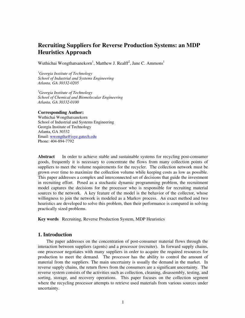
decision in each decision period. This decision affects the decisions of the agents. It is assumed that the willingness state of each agent is updated to the recruiter in every period. Also, the total spending budget in all periods must not exceed the total recruiting budget limit provided to the recruiter at the beginning of planning period. At the beginning of the period, after an agent receives its allocation of budget (Resource A) from the recruiter, it decides whether to give/sell its resource, Resource B, to the recruiter. Its decision is based on its willingness to part with the resource. In the case where the agent does not contract to provide the resource to the recruiter, the agent’s overall willingness state can change by being influenced by the incentives it receives from the recruiter. Figure 2 summarizes how the decision of the recruiter is related to the decision of the agents in each period.

Figure 2: Decisions of Recruiter and Agent in One Period

A key element of our recruitment framework is a model of an agent’s willingness to

participate. This model can be as simple as a one-variable function of the given incentive. However, it is more likely that agents have a more sophisticated “state” relative to their willingness to participate. A Markov model for the agent, which we call the Agent’s Resource Willingness Model (ARW), is developed in order to capture a more sophisticated structure of the agent behavior and yet retain reasonable representational and computational simplicity. Agent’s Resource Willingness Model (ARW)

The significant components of this model are the willingness state and the transition probabilities. We model each agent’s resource willingness as a Markov chain with a “recruited” state that is absorbing. This means that the recruited agent never leaves the collection network and the recruiter is not confronted with an agent retention issue. The model also consists of other states that represent a “distance” from recruitment based on the

Starting Budget

Agent 1 Agent � Agent 2

Recruiter

Agent 3

Recruiter’s Decision

Agent’s Decision

Agent 1 Agent � Agent 2 Agent 3

Join Network

Join Network

5

probability of reaching recruitment and connection to other states. Each agent has its own Markov model and it is assumed the recruiter knows the state of the agent in each time period. Consider agent i in this model.

Willingness State Definition (Agent’s state)

{ , , , }its R L M H� .

This describes what state agent i is in at time period t . There are four possible states for each agent:

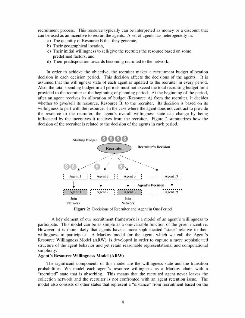
1. Recruited (R) - The agent agrees to give the Resource B to the recruiter. 2. Low (L) - The agent is not recruited by the recruiter. Also, the agent is in a state where it will be very challenging to recruit it. 3. Medium (M) - The agent is not recruited by the recruiter. The agent has no bias against the recruitment. 4. High (H) - The agent is not recruited by the recruiter. Also, the agent is in a state that makes recruitment easy.

We assume that when an agent is recruited, it resides in the R willingness state, an absorbing state. The states L, M, and H represent a “distance” from recruitment based on the probability of reaching the recruitment state and connection to other states. In other words, if the agent is not recruited, it resides in either the L, M, or H state. Figure 3 shows a symbolic representation of the states and possible transitions.

Figure 3: Agent’s State Diagram

We denote the amount of Resource B that agent i can generate between each decision

epoch (each period) as ig , which is assumed to be a single value, although it would not be difficult to generalize it to a random variable. We also assume that the recruiter can collect the full amount of available Resource B from every recruited retailer in each period. In addition, we denote ita as the amount of budget (Resource A) that agent i receives from the recruiter in period t . Given the action ita , the agent transits to the next state with following transition probabilities.

Transition Probabilities

The probability of agent i moving to state , 1i ts � from state its by action ita is denoted by

, 1( | , )i t it itp s s a� or , 1

( )it i ts s itPr a

�. There are two types of transition probabilities to consider.

H M L

R Probability =1

6

The probability of recruitment is the probability of moving to state R from the L M, or H states ( ( ), ( ), ( )LR it MR it HR itPr a Pr a Pr a ). The difficulty of recruitment depends on three factors: the state of the agent, the budget allocation or action, and the agent’s recruitment budget threshold, i� . The recruitment budget threshold has the same units as the Resource A budget allocation. In general, it represents a minimum value required to recruit the agent. In the case of carpet retailers, there may be some correlation between the size of the retailer and the budget threshold required because the incentives offered may directly scale with the amount of used carpet available for pick-up. The threshold may be interpreted as subsidizing the cost of the retailer’s disposal fee. In section 5, when we provide the data for numerical study, we assume that if the agent can provide a significant amount of Resource B, it also demands large amount of allocation of Resource A from the recruiter. Thus, the recruitment budget threshold depends on the amount of Resource B collection volume available from agent i . A higher ig implies a higher i� . This means that it is more expensive to recruit agents who have higher Resource B generation rates.

In order to capture these three factors together, we apply a sigmoid function (Seggern 1993) to calculate the probability of recruitment. In addition, we define the recruitment willingness factor, s� , based on the state of the agent such that 0H M L� � �� .

The sigmoid function to calculate probability of recruitment of agent i at time t is:

( )

1( )

1it s it iits R it aPr a

e � ��

. (1)

Using the probability of recruitment function in (1), we can vary the value of the recruitment willingness factor so that each state has different recruitment probabilities as shown in Figure 4. We set 2H� � , 1M� � , and 0.5L� � , with i� =0 for all states.

0

0.5

1

-9 -6 -3 0 3 6 9

Pro

babl

ity o

f Rec

ruitm

ent H

M

L

Figure 4: Recruitment Probability for Different Recruitment Willingness States

The probability of (unrecruited) state transition can be specified according to how

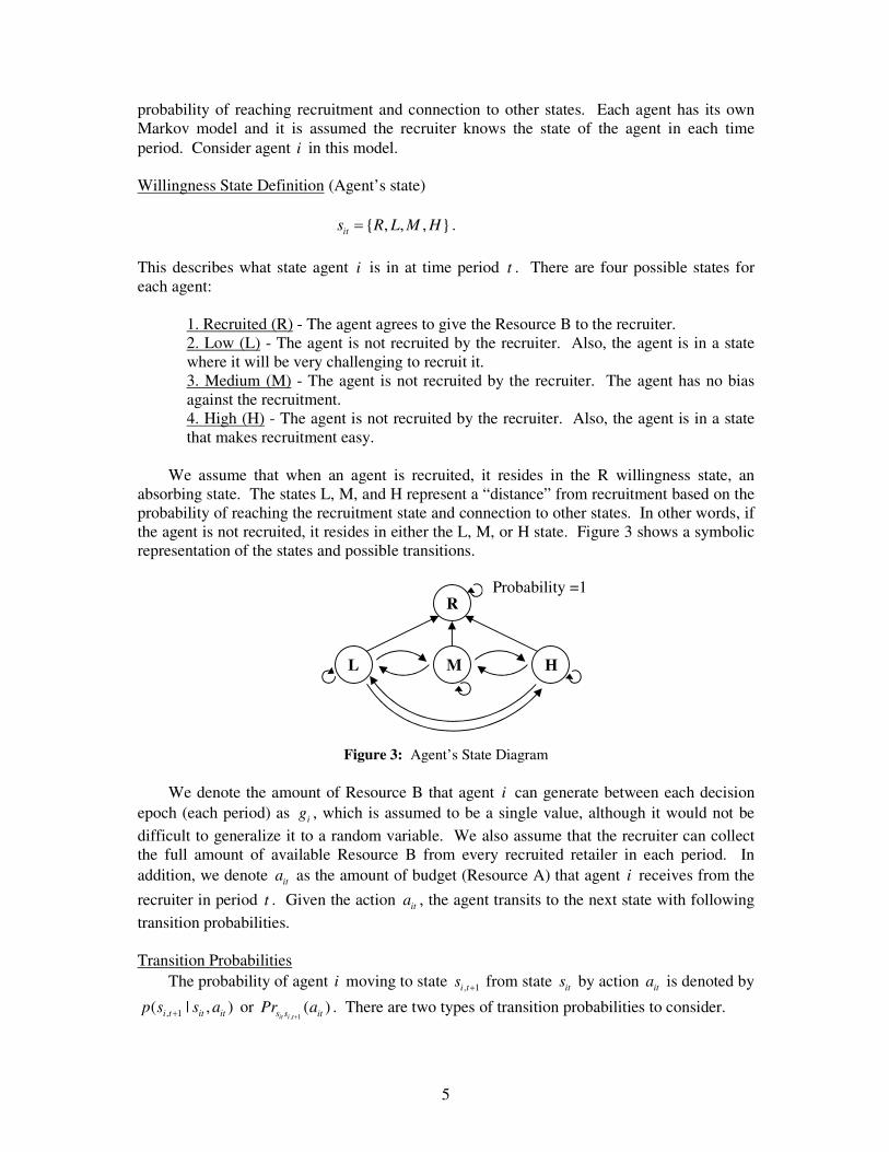
readily a particular agent is moved among the L, M, and H states if it is not recruited. The probability of state transitions can be set up such that it is easy to move to M and H from L. This makes the agent easier to recruit. On the other hand, the probability of state transition can be set up such that it is more difficult to move to M and H from L. This makes the agent more difficult to recruit. Figure 5 displays the overall transition probabilities of an agent.

ita

7

Figure 5: Transition Probabilities for an Agent

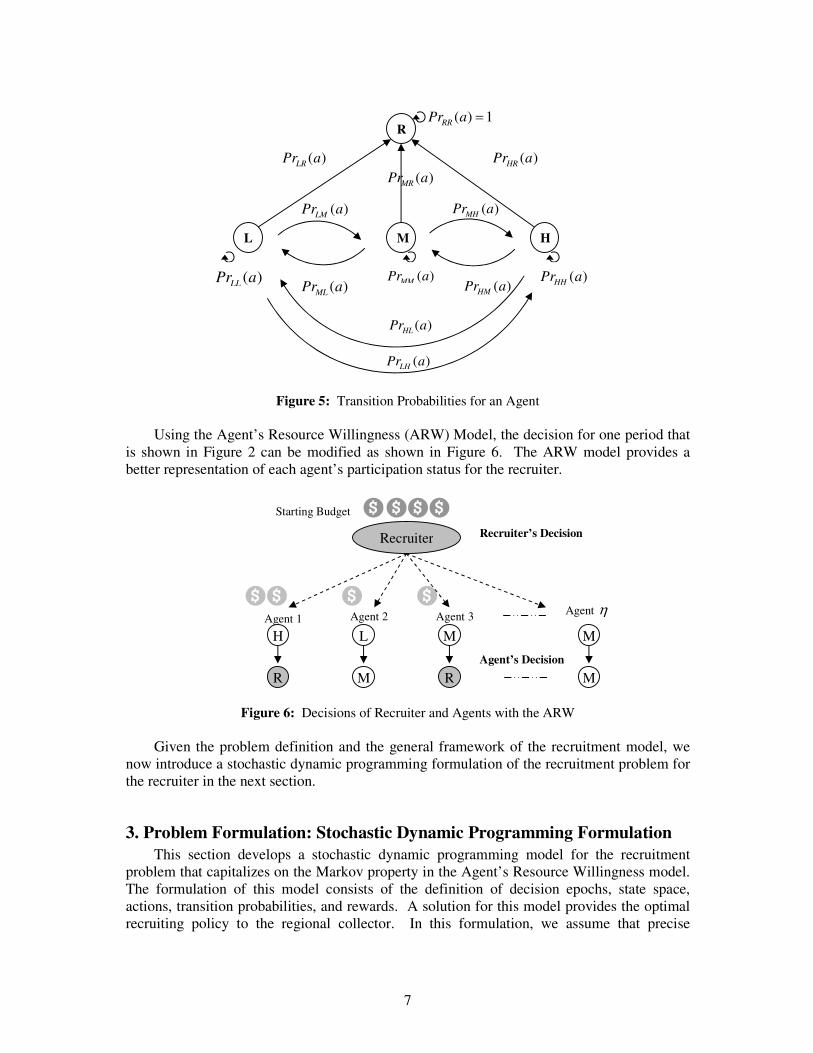
Using the Agent’s Resource Willingness (ARW) Model, the decision for one period that

is shown in Figure 2 can be modified as shown in Figure 6. The ARW model provides a better representation of each agent’s participation status for the recruiter.

Figure 6: Decisions of Recruiter and Agents with the ARW

Given the problem definition and the general framework of the recruitment model, we now introduce a stochastic dynamic programming formulation of the recruitment problem for the recruiter in the next section.

3. Problem Formulation: Stochastic Dynamic Programming Formulation This section develops a stochastic dynamic programming model for the recruitment

problem that capitalizes on the Markov property in the Agent’s Resource Willingness model. The formulation of this model consists of the definition of decision epochs, state space, actions, transition probabilities, and rewards. A solution for this model provides the optimal recruiting policy to the regional collector. In this formulation, we assume that precise

Starting Budget

Agent 1 Agent � Agent 2

Recruiter

Agent 3

Recruiter’s Decision

Agent’s Decision

H

R

M

R

L

M

M

M

( ) 1RRPr a �

( )HLPr a

( )LHPr a

( )MRPr a

( )MHPr a( )LMPr a

H M L

R

( )MMPr a( )LLPr a ( )MLPr a ( )HMPr a( )HHPr a

( )LRPr a ( )HRPr a

8

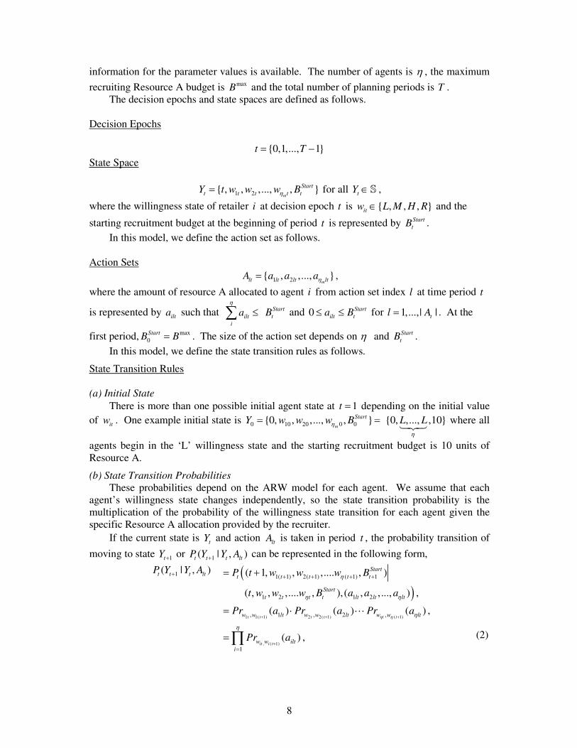
information for the parameter values is available. The number of agents is � , the maximum recruiting Resource A budget is maxB and the total number of planning periods is T .

The decision epochs and state spaces are defined as follows.

Decision Epochs

{0,1,..., 1}t T� � State Space

1 2{ , , ,..., , }m

Startt t t t tY t w w w B�� for all tY � ,

where the willingness state of retailer i at decision epoch t is { , , , }itw L M H R and the

starting recruitment budget at the beginning of period t is represented by StarttB .

In this model, we define the action set as follows.

Action Sets

1 2{ , ,..., }mlt lt lt ltA a a a�� ,

where the amount of resource A allocated to agent i from action set index l at time period t

is represented by ilta such that ilti

a�

� StarttB and 0 Start

ilt ta B for 1,...,| |tl A� . At the

first period, max0StartB B� . The size of the action set depends on � and Start

tB . In this model, we define the state transition rules as follows.

State Transition Rules

(a) Initial State There is more than one possible initial agent state at 1t � depending on the initial value

of itw . One example initial state is 0 10 20 0 0{0, , ,..., , }m

StartY w w w B�� {0, ,..., ,10}L L�

�� where all

agents begin in the ‘L’ willingness state and the starting recruitment budget is 10 units of Resource A.

(b) State Transition Probabilities These probabilities depend on the ARW model for each agent. We assume that each

agent’s willingness state changes independently, so the state transition probability is the multiplication of the probability of the willingness state transition for each agent given the specific Resource A allocation provided by the recruiter.

If the current state is tY and action ltA is taken in period t , the probability transition of moving to state 1tY � or 1( | , )t t t ltP Y Y A� can be represented in the following form,

1( | , )t t t ltP Y Y A� � 1( 1) 2( 1) ( 1) 1( 1, , ,.... , )Startt t t t tP t w w w B��

1 2 1 2( , , ,.... , ), ( , ,..., )Startt t t t lt lt ltt w w w B a a a� � ,

1 1( 1) 2 2( 1) ( 1), 1 , 2 ,( ) ( ) ( )

t t t t t tw w lt w w lt w w ltPr a Pr a Pr a� � ��

� � �� ,

, ( 1)

1

( )it i tw w ilt

i

Pr a�

��

�� , (2)

9

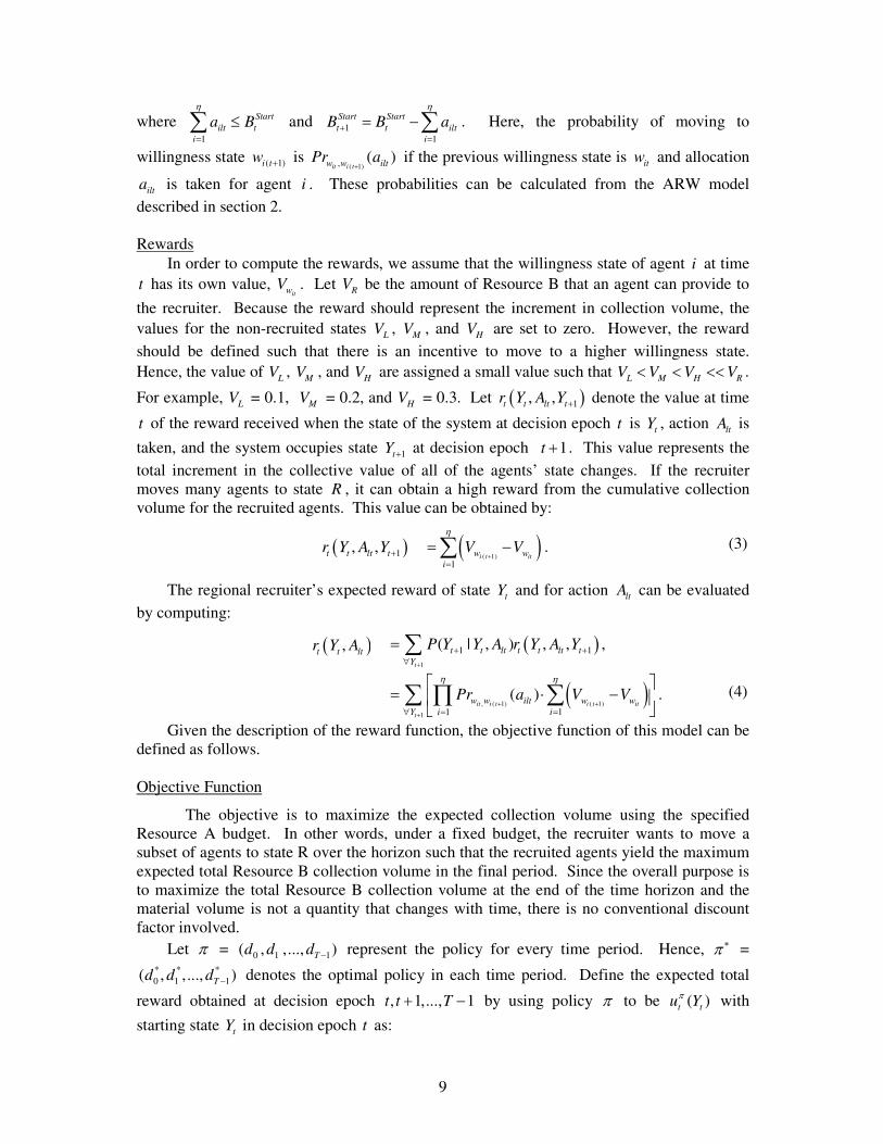
where 1

Startilt t

i

a B�

�

� and 11

Start Startt t ilt

i

B B a�

��

� �� . Here, the probability of moving to

willingness state ( 1)i tw � is ( 1), ( )

it i tw w iltPr a�

if the previous willingness state is itw and allocation

ilta is taken for agent i . These probabilities can be calculated from the ARW model described in section 2. Rewards

In order to compute the rewards, we assume that the willingness state of agent i at time t has its own value,

itwV . Let RV be the amount of Resource B that an agent can provide to the recruiter. Because the reward should represent the increment in collection volume, the values for the non-recruited states LV , MV , and HV are set to zero. However, the reward should be defined such that there is an incentive to move to a higher willingness state. Hence, the value of LV , MV , and HV are assigned a small value such that L M H RV V V V� � �� .

For example, LV = 0.1, MV = 0.2, and HV = 0.3. Let � 1, ,t t lt tr Y A Y � denote the value at time

t of the reward received when the state of the system at decision epoch t is tY , action ltA is taken, and the system occupies state 1tY � at decision epoch 1t � . This value represents the total increment in the collective value of all of the agents’ state changes. If the recruiter moves many agents to state R , it can obtain a high reward from the cumulative collection volume for the recruited agents. This value can be obtained by:

� 1, ,t t lt tr Y A Y � � ( 1)1

i t itw wi

V V�

��

� �� . (3)

The regional recruiter’s expected reward of state tY and for action ltA can be evaluated by computing:

� ,t t ltr Y A � 1

1 1( | , ) , ,t

t t lt t t lt tY

P Y Y A r Y A Y�

� ��

� � ,

� , ( 1) ( 1)

1 11

( )it i t i t it

t

w w ilt w wY ii

Pr a V V� �

� �

��

� ��

� �� . (4)

Given the description of the reward function, the objective function of this model can be defined as follows.

Objective Function

The objective is to maximize the expected collection volume using the specified Resource A budget. In other words, under a fixed budget, the recruiter wants to move a subset of agents to state R over the horizon such that the recruited agents yield the maximum expected total Resource B collection volume in the final period. Since the overall purpose is to maximize the total Resource B collection volume at the end of the time horizon and the material volume is not a quantity that changes with time, there is no conventional discount factor involved.

Let � = 0 1 1( , ,..., )Td d d � represent the policy for every time period. Hence, � � = * * *0 1 1( , ,..., )Td d d � denotes the optimal policy in each time period. Define the expected total

reward obtained at decision epoch , 1,..., 1t t T� � by using policy � to be ( )t tu Y� with starting state tY in decision epoch t as:

10

1

( ) ( , )t

T

t t Y t t ltt t

u Y E r Y A� ��

� � ��

� ��

� � . (5)

Let *( )t tu Y denote the maximum expected total reward obtained at decision epochs

, 1,.., 1t t T� � with starting state tY in decision epoch t . Then the optimality equation for the recruitment problem is:

�1

* * *1 1 1( ) ( ) max ( , ) ( | , ) ( )

tlt

t t t t t t lt t t t lt t tYA

u Y u Y r Y A P Y Y A u Y�

�

� � ��

� �! !� � ��

! !� � , (6)

1

* *1 1 1( ) arg max ( , ) ( | , ) ( )

tlt

t t t lt t t t lt t tYA

A Y r Y A P Y Y A u Y�

� � ��

� �! !� ��

! !� ��

. (7)

The optimal action in states Y at epoch t is denoted by *( )tA Y . In other words, the

maximum expected total reward at period t , *( )t tu Y , is the realization from all possible actions of the immediate reward and expected future reward from a particular action. Essentially, the objective of the recruitment problem is to find *

0 0( )u Y . We have not found a similar formulation in the literature. The formulation that appears

closest is the restless bandit problem. Bertsimas and Nino-Mora (2000) addresses the restless bandit problem as follows. Consider a total of N � projects, named {1,2,..., }n N N� � � � . Project n�can be in one of a finite number of states ' '

n ni I . At 0,1,2,...,t � exactly M N� ��

projects must be chosen to work on or set active. If project n� , in state 'ni , is active, an active

reward '1

niR is received, and its state transition change follows from an active transition

probability matrix into state 'nj with probability ' '

1

n ni jP . On the other hand, if project is not

worked on, a passive reward '0

niR is earned, and its state transition change follows from an

passive transition probability matrix into state 'nj with probability ' '

0

n ni jP . Rewards are time-

discounted by a specific discount factor. The problem’s objective is to find a scheduling policy that maximizes the total expected discounted reward over an infinite horizon.

Our recruitment problem formulation is a generalization of the restless bandits to include (1) more possible actions for each selected bandit other than just selection or not, and (2) an overall budget constraint. First, the recruitment problem’s number of actions for each agent or project can be greater than the two in the restless bandit problem (active and passive). Second, the restless bandit problem has one linking constraint which is exactly M projects must be worked on, or set active. In contrast, we cannot fix how many agents are worked on in each time period. Instead, we have the budget linking constraint which limits the action set in later periods. In addition, the restless bandits do not have internal state, whereas our "agents" do have internal state (R,L,M,H) which they remember from one period to the next. This latter generalization of inter-period coupling is significant because the coupling between time periods is therefore not just via the budget constraints but also through the state equations.

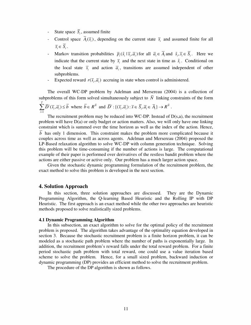
Furthermore, our recruitment problem has some similarities to the weakly coupled dynamic program (WC-DP) introduced by Adelman and Mersereau (2004). The problem description of WC-DP is as follows. There are I subproblems that are each Markov decision problems on disjoint state spaces. Corresponding to subproblem i , define the following:

11

- State space iS , assumed finite

- Control space ( )i iA s , depending on the current state is and assumed finite for all

i is S .

- Markov transition probabilities ( | , )i i i ip s s a� for all i ia A and ,i i is s S� . Here we indicate that the current state by is and the next state in time as is� . Conditional on the local state is and action ia , transitions are assumed independent of other subproblems.

- Expected reward ( , )i ir s a accruing in state when control is administered. The overall WC-DP problem by Adelman and Mersereau (2004) is a collection of

subproblems of this form solved simultaneously subject to N linking constraints of the form

1

( , )I

ii i

i

D s a b�

� where Nb R and :{( , ) : , }i Ni i i i iD s a s S a A R " .

The recruitment problem may be reduced into WC-DP. Instead of D(s,a), the recruitment problem will have D(a) or only budget or action matters. Also, we will only have one linking constraint which is summed over the time horizon as well as the index of the action. Hence, b has only 1 dimension. This constraint makes the problem more complicated because it couples across time as well as across agents. Adelman and Mersereau (2004) proposed the LP-Based relaxation algorithm to solve WC-DP with column generation technique. Solving this problem will be time-consuming if the number of actions is large. The computational example of their paper is performed over derivatives of the restless bandit problem where the actions are either passive or active only. Our problem has a much larger action space.

Given the stochastic dynamic programming formulation of the recruitment problem, the exact method to solve this problem is developed in the next section.

4. Solution Approach In this section, three solution approaches are discussed. They are the Dynamic

Programming Algorithm, the Q-learning Based Heuristic and the Rolling IP with DP Heuristic. The first approach is an exact method while the other two approaches are heuristic methods proposed to solve realistically sized problems.

4.1 Dynamic Programming Algorithm

In this subsection, an exact algorithm to solve for the optimal policy of the recruitment problem is proposed. The algorithm takes advantage of the optimality equation developed in section 3. Because the stochastic recruitment problem is a finite horizon problem, it can be modeled as a stochastic path problem where the number of paths is exponentially large. In addition, the recruitment problem’s reward falls under the total reward problem. For a finite period stochastic path problem with total reward, one could use a value iteration based scheme to solve the problem. Hence, for a small sized problem, backward induction or dynamic programming (DP) provides an efficient method to solve the recruitment problem.

The procedure of the DP algorithm is shown as follows.

12

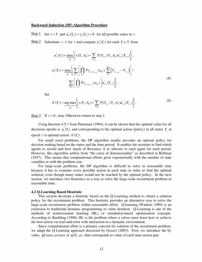
Backward Induction (DP) Algorithm Procedure Step 1 Set t T� and * ( ) ( ) 0T T T Tu Y r Y� � for all possible states in t .

Substitute 1t � for t and compute *( )t tu Y for each tY � from

�1

* *1 1 1( ) max ( , ) ( | , ) ( )

tlt

t t t t lt t t t lt t tYA

u Y r Y A P Y Y A u Y�

� � ��

� �! !� ��

! !� � ,

� � , ( 1) ( 1)

1

*

11

( ) max ( )m

it i t i t it

tlt

t t w w ilt w wY iA i

u Y Pr a V V��

� �

��

� � �!� � � ��

! � ��

, ( 1)

1

*1 1

1

( ) ( )it i t

t

w w ilt t tY i

Pr a u Y�

�

�

� ��

�# $ !�% &!' (

� � . (8)

Step 2

Set

1

* *1 1 1( ) arg max ( , ) ( | , ) ( )

tlt

t t t lt t t t lt t tYA

A Y r Y A P Y Y A u Y�

� � ��

� �! !� ��

! !� ��

. (9)

Step 3 If 0t � , stop. Otherwise return to step 2. Using theorem 4.5.1 from Puterman (1994), it can be shown that the optimal value for all

decisions epochs is *( )t tu Y and corresponding to the optimal action (policy) in all states tY at

epoch t is optimal action *( )tA Y . For small sized problems, the DP algorithm readily provides an optimal policy for

decision making based on the states and the time period. It enables the recruiter to find which agents to recruit and how much of Resource A to allocate to each agent for each period. However, this algorithm suffers from “the curse of dimensionality” as described in Bellman (1957). This means that computational efforts grow exponentially with the number of state variables or with the problem size.

For large-scale problems, the DP algorithm is difficult to solve in reasonable time because it has to examine every possible action in each state in order to find the optimal solution, even though many states would not be reached by the optimal policy. In the next section, we introduce two heuristics as a way to solve the large-scale recruitment problem in reasonable time.

4.2 Q-Learning Based Heuristic

This section develops a heuristic based on the Q-Learning method to obtain a solution policy for the recruitment problem. This heuristic provides an alternative way to solve the large-scale recruitment problem within reasonable effort. Q-learning (Watkins 1989) is an extension to traditional dynamic programming or value iteration. Q-Learning is one of the methods of reinforcement learning (RL) or simulation-based optimization concepts. According to Kaebling (1996), RL is the problem where a solver must learn how to achieve the best action via trial-and-error with interaction in a dynamic environment.

Since computational effort is a primary concern for solution of the recruitment problem, we adapt the Q-Learning approach discussed by Gosavi (2003). First, we introduce the Q-value, ( , )Q state action or ( , )tQ Y a , that corresponds to value of each state-action pair.

13

The step-by-step procedure of the Q-Learning Based Heuristic (QBH) procedure is shown as follows.

Q-Learning Based Heuristic (QBH) Procedure

Step 0 Set the iteration number to 0. Select a value for ) where 0 1) and initialize the iteration limit.

Step 1 Initialize time period, t , to 0 and starting state to tY . This represents the initial budget and initial willingness state of each agent.

Step 2 Generate an action a using an action selection heuristic, described below.

Step 3 Simulate action a to retrieve the next period action, 1tY � . Let 1( , , )t t tr Y a Y � be the immediate reward earned in the transition to state 1tY � from state tY under the influence of action a . Update ( , )tQ Y a using the following equation:

11 1( )

( , ) (1 ) ( , ) [ ( , , ) max ( , )]t

t t t t t tb A YQ Y a Q Y a r Y a Y Q Y b) )

��

* � � � , 0 1)� , (10)

Step 4

where 1( )tA Y � represent all possible actions in state 1tY � and if 1( , )tQ Y b� has no value, set its initial value is set to 0.

Step 5 If t T� , increase t by 1 and go to step 2. Else, increase the iteration number by 1. If the iteration number exceeds the limit, go to step 6. Else, increase t by 1 and go to step 2.

Step 6 For each tY , select

( )

( ) arg max ( , )t

t t

b A Y

A Y Q Y b�

��

. (11)

The learning rate is represented by ) in (10). Its value weights how much the previous value of ( , )tQ Y a and the evaluation of immediate reward with future reward should affect the new value of ( , )tQ Y a . The Q-value is a prediction of the sum of the reinforcement one receives when performing the associated action and the following given policy. To update the prediction ( , )tQ Y a , one must perform the associated action a, causing a transition to the next state 1tY � , and returning a scalar reinforcement 1( , , )t t tr Y a Y � . Then one only needs to find the maximum Q-value in the new state,

11( )

max ( , )t

tb A YQ Y b

��

, to have all necessary

information for revising the prediction (Q-Value) associated with the action just performed. Q-learning does not require one to calculate the transition probabilities to successor states. The reason is that a single sample or a successor state for a given action is an unbiased estimate of the expected value of the successor state.

The action selection heuristics in step 2 of the QBH procedure are described as follows.

14

Action Selection Heuristics

Budget allocation for each agent represents the action a in step 2 of the QBH. It is very important to select an action wisely as this is the exploration part of the RL. Three heuristics are introduced as follows. In the Q-Learning QBH procedure, one of the heuristics is randomly selected during each execution of action selection.

Heuristic 1: Random Allocation

In this heuristic, the remaining budget is allocated to a random set of agents at a random amount level.

Heuristic 2: High Willingness State Agent First

This heuristic focuses on allocating the remaining budget to those agents who have a higher chance of recruitment success. This may not be the best way to obtain the highest payoff because the agents with a high willingness state may generate smaller amount of Resource B collection volume compared to agents with a low willingness state who generate a higher amount of collection volume. Heuristic 3: High Collection Volume Agent First

This heuristic focuses on allocating the remaining budget among those agents who generate higher amount of Resource B collection volume. This may not be the best way to obtain the highest payoff because agents with a higher collection volume may be very hard to recruit. In other words, recruiting many willing small agents may result in a higher amount of total collection volume.

The QBH uses the action selection heuristics to explore the action and state spaces. The

exploitation applies (10) to update the Q-value for a state-action pair. According to Gosavi (2003), the Q-Learning method gives a near-optimal solution when the maximum number of iterations is large enough.

In order to perform a large number of iterations in a reasonable computation time, the computational complexity of the algorithm should be analyzed. In step 4, the number of steps required to update ( , )tQ Y a in (10) requires first a search for the initial value of ( , )tQ Y a and second the maximization of 1( , )tQ Y b� for every value of 1( )tb A Y � . The value look-up for ( , )tQ Y a is performed in ( )O + steps, where + is the size of a typically large Q-table. A Q-table is a look-up table that stores the value of ( , )Q state action for every encountered state-action pair. This step takes ( )O + , number of actions at states 1tY � , which is typically large. In summary, every computation of (10) in step 4 of the Q-Learning Based Heuristic requires:

Time Complexity of (10) = ( ) | |O A+ � . (12)Two modifications are introduced to speed up this step. The first is to set the learning rate ) equal to 1 and the second is to store the Q-values using a hash table. Each of these modifications is described in the following paragraphs. Learning Rate Equal to One

With ) = 1, equation (10) becomes

11 1( )

( , ) ( , , ) max ( , )t

t t t t tb A YQ Y a r Y a Y Q Y b

��

* � . (13)

15

Instead of storing 1( , )tQ Y b� for every value of 1( )tb A Y � and searching for the maximum of

11( )

max ( , )t

tb A YQ Y b

��

in every iteration, it is much simpler to store the maximum of 1( , )tQ Y b� into

max 1 max( , )tQ Y b� . Under this modification, the update of ( , )tQ Y a becomes:

max max max max 1 max 1 max( , ) max[ ( , ), ( , , ) ( , )]t t t t t tQ Y a Q Y a r Y a Y Q Y b� �� . (14)Basically, retrieving

11( )

max ( , )t

tb A YQ Y b

��

can be done in complexity of ( )O + by looking up

max 1 max( , )tQ Y b� . The update of max max( , )tQ Y a is performed if the new value of

1 max 1 max( , , ) ( , )t t t tr Y a Y Q Y b� �� is higher than the previous value of max max( , )tQ Y a . In this step, the best action maxa is also updated accordingly.

In addition to this modification, the Hash Table data structure is applied to the QBH method. It is described as follows.

Hash Table

The QBH method requires a large Q-table in order to retrieve Q-values of corresponding states and actions. Computationally, it is time-consuming to retrieve the selected Q-value using a traditional array for the data-structure. As a better alterative, Hash Tables (Knuth 1973) are used as a Q-value data structure to improve the look-up time. The Q-value can be retrieved in complexity of (1)O in the average case and best cases. The worst case search time is ( )O + ; however, the probability of this happening is vanishingly small. This data structure technique does not have an impact on the solution quality of the QBH method. The procedure is the same. The only change is the retrieval time of the Q-value of any state-action pair in (10).

Employing the hash table data structure for Q-values and fixing the learning rate ) to one, the computational complexity of (10) in step 4 of the QBH is reduced from ( ) | |O A+ � to (1)O in the average and best cases. In the worst case, it is ( )O + . This improvement reduces computational requirements for exploitations. Completely ignoring the previous value of Q-value by setting the learning rate ) to one may affect the resulting quality of the heuristic solution, but the computational effort is significantly reduced to facilitate overall problem solution.

4.3 A Rolling IP with DP Heuristic

As an alternative to the QBH procedure, a heuristic employing integer programming (IP) has been explored. The heuristic is based on an observation of the DP algorithm described in section 4.1. An optimal recruitment policy for an individual agent can be found using the DP algorithm because the number of states and actions is small. This characteristic may be exploited to solve the overall recruitment problem. The main concept of this heuristic is to shrink a multi-period problem so as to think of it a one-period problem. First, the optimal policy for each individual agent is solved for T periods using the DP algorithm. Then, all of these individual agent solutions are used to find the best combination of budget allocations among agents. The resulting solution is implemented for the first time period where the selected agents receive their given first period budget allocations. Next, the optimal policy for each individual agent is solved for the remaining 1T � periods. Then the procedure repeats itself until the final period is solved. The example of an agent for whom a recruitment budget is allocated in the first and second period is shown in Figure 7.

16

Figure 7: The Rolling Horizon Concept

A key step in this approach is an optimization problem that selects the best combination of individual policies to use to maximize the collective recruited agents’ collection volume, subject to the overall recruitment budget constraint. This approach is suboptimal because it does not take advantage of the ability to observe and respond to recruitment during the policy execution. To improve performance, a rolling horizon implementation is applied. The remaining unspent funds allocated to those agents who have been recruited and unspent funds allocated to retailers not recruited are added back to the available recruitment budget amount and then the optimization problem is resolved with the updated information.

The reason why this approach is suboptimal is because it does not take an action based on the information about how the retailers respond to the expenditures. It allocates a budget to be spent for the entire period on the retailer and only reactively reallocates money from among retailers who are recruited early on in the process.

The stochastic recruitment function is denoted by max( , , )SR i B t as a function that returns the solution from solving the recruitment problem with the DP algorithm (developed in section 4.1) for retailer i for t periods given the starting total budget maxB . The solution yields the optimal budget allocation policy in each period and the expected collection volume from retailer i over t periods. Next, the optimization problem that selects the best combination of individual policies among all retailers is formulated. In order to limit the problem size, we discretize the budget parameter in the formulation. The index, parameters, and variables are defined as: Index: i Index of agents ( i = 1, 2, …, m� ) j Index of budget levels ( j = 1, 2, …, J )

Parameters:

maxB Maximum starting total budget over total T periods starttB Maximum starting budget at period t

jb Budget allocation the collector choose to spend on the retailer, which is the value of thj entry in 1( ,..., ,..., )j JB b b b�

ijv� Maximum expected increment of capacity volume that can be collected from retailer i if budget amount jb is allocated to that retailer. The value of ijv� can be

obtained from solving ( , , )jSR i b t using the DP approach.

Optimal Policy for 1 period

If allocated, spend budget in the first period

If allocated, spend budget in the second

Optimal Policy for 2 periods

17

Decision Variables:

ijx = ��

1 if budget amount jb is allocated to retailer i 0 otherwise

The integer programming problem denoted the Rolling IP for period t can be formulated as: Rolling IP ( )tRP for Period t Maximize

ij iji j

v x�� (15)

Subject to: 1ijj

x � i� (16)

start

j ij ti j

b x B�� (17)

{0,1}ijx � ,i j� . (18)

The objective function (15) is the sum of collection volume. Constraints (16) permit only one budget amount to be allocated to retailer i . Constraint (17) restricts the overall spending budget to be less than the budget limit. Constraints (18) force ijx variables as binary variables.

The procedure for the Rolling IP with DP method is discussed next by combining the Rolling IP formulation together with the rolling horizon concept.

Rolling IP with DP Heuristic (RIDH) Solution Procedure Step 0 Set 1t � and max

0startB B� .

Solve for ijv� from ( , , )jSR i b T as defined earlier in this section for all agents i and

budget level j using the DP approach developed in section 4.1. The initial state of ( , , )jSR i b T is [0, initial willingness state of retailer i , jb ].

Step 1 Formulate the rolling IP ( )tRP model and solve for ijx .

Step 2 For the retailers for where a recruiting budget has been allocated, simulate the action in period t only. If t T� , obtain the total increment in collection volume from period 1 to period T and exit. Otherwise, go to Step 3.

Step 3 Set 1t t� � .

Update the value of ijv� from for all ,i j . Note that there is no need to resolve

MDP for each retailer. Obtain the ijv� by changing the starting initial state to [t+1, new willingness state, remaining budget]. For example, if the initial state is [0,M,30], a budget amount 10 is applied to this period, the next period status change to H, and the overall remaining budget is 10, then ijv� can be looked up

18

from state [1,H,10]. Update remaining budget start

tB , ( 1start startt tB B �� actual budget spent in the

previous period). Go to Step 1

These steps can be summarized by the flow chart shown in Figure 8.

Figure 8: Procedure for the RIDH Solution Approach

5. Computational Results In this section, the alternative solution approaches are applied to small and large

examples. Since the DP algorithm can find an optimal solution for a small example in a reasonable computation time, its solution can be used as a benchmark against the solutions obtained by the RIDH, and QBH. For the large example, the computational requirements are prohibitive for the DP algorithm. Thus, only the results from the two heuristics are compared. All the computation experiments are solved using a Windows 2000-based Pentium 4 1.80 GHz personal computer with 640MB of RAM with CPLEX version 8.0 (www.ilog.com) for the optimization software.

5.1 Small Example For our small example, the recruitment willingness factors for the willingness state of

each retailer are defined as 2H� � , 1M� � , and 0.5L� � . Equation (1) is used to compute the probabilities of recruitment, ( ( )LRPr a , ( )MRPr a , ( )HRPr a ), for the given willingness state and budget allocation ( a ). If recruitment does not occur, then there is still the chance the state of retailer will change. This also depends on the recruitment budget threshold of the

Set 0t �

Obtain final result

Obtain the value for all ijv�

Formulate and solve IP ( )tRP

Simulate and update the actual state of each retailer.

Set 1t t� �

t T�

No

Yes

Update remaining budget and ijv�

19

retailer. When the given budget allocation fails to recruit the retailer, two cases are considered.

Case A: If ia �- , the transition probabilities are depicted in Figure 9.

Figure 9: Transition Probabilities for Case A

Case B: If 0 ia � � , the transition probabilities are depicted in Figure 10.

Figure 10: Transition Probabilities for Case B

With these settings, we generate four test cases that have different retailers’ initial

willingness states as shown in Table 1. Table 2 shows the amount of collection capacity and recruitment budget threshold of each retailer. The alternative budget limitation settings are spaced 10 units apart 10, 20, …, 100 and the budget allocation settings are similarly spaced. The number of time periods is chosen to be three. From the collective retailer collection capacities, the maximum system collection capacity in all these four cases is 220 pounds, over a given time period.

Table 1: Small Example Data

Case Initial Willingness State

1 LLLLL 2 MMMMM 3 HHHHH 4 MHHMH

0.1 0 0.1

0

0

0.9 0.9

H M L

0.1 0.9

0.4 0.3

0.4 0.6

H M L

0.3 0.4 0.6

0

0

20

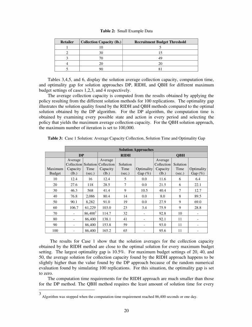
Table 2: Small Example Data

Retailer Collection Capacity (lb.) Recruitment Budget Threshold 1 10 5 2 30 15 3 70 49 4 20 20 5 90 81

Tables 3,4,5, and 6, display the solution average collection capacity, computation time,

and optimality gap for solution approaches DP, RIDH, and QBH for different maximum budget settings of cases 1,2,3, and 4 respectively.

The average collection capacity is computed from the results obtained by applying the policy resulting from the different solution methods for 100 replications. The optimality gap illustrates the solution quality found by the RIDH and QBH methods compared to the optimal solution obtained by the DP algorithm. For the DP algorithm, the computation time is obtained by examining every possible state and action in every period and selecting the policy that yields the maximum average collection capacity. For the QBH solution approach, the maximum number of iteration is set to 100,000.

Table 3: Case 1 Solution: Average Capacity Collection, Solution Time and Optimality Gap

Solution Approaches

DP RIDH QBH

Maximum Budget

Average Collection Capacity

(lb.)

Solution Time (sec.)


(lb.)


Optimality Gap (%)


(lb.)


Optimality Gap (%)

10 12.4 16 12.4 5 0.0 11.6 6 6.4 20 27.6 118 28.5 7 0.0 21.5 6 22.1 30 46.3 568 41.4 9 10.5 40.4 7 12.7 40 76.8 2,086 80.4 14 0.0 8.0 8 89.5 50 90.1 8,282 91.0 19 0.0 27.9 9 69.0 60 106.7 61,229 103.0 23 3.4 75.9 9 28.8 70 - 86,4003 114.7 32 - 92.8 10 - 80 - 86,400 138.1 41 - 92.1 11 - 90 - 86,400 153.8 59 - 93.0 11 -

100 - 86,400 165.2 65 - 95.6 11 -

The results for Case 1 show that the solution averages for the collection capacity obtained by the RIDH method are close to the optimal solution for every maximum budget setting. The largest optimality gap is 10.5%. For maximum budget settings of 20, 40, and 50, the average solution for collection capacity found by the RIDH approach happens to be slightly higher than the value found by the DP approach because of the random numerical evaluation found by simulating 100 replications. For this situation, the optimality gap is set to zero.

The computation time requirements for the RIDH approach are much smaller than those for the DP method. The QBH method requires the least amount of solution time for every 3

Algorithm was stopped when the computation time requirement reached 86,400 seconds or one day.

21

maximum budget setting, but the optimality gap is larger than that found by the RIDH approach. In fact, its solution is worse than solution obtained by the RIDH approach for every maximum budget setting. For maximum budget settings of 80 to 100, the DP method cannot obtain optimal policy within the stopping time limit of one day of computational effort.


Solution Approaches

DP RIDH QBH

Maximum Budget


(lb.)



(lb.)


Optimality Gap (%)


(lb.)


Optimality Gap (%)

10 12.2 1 12.6 4 0.0 1.5 6 87.7 20 47.2 8 44.4 6 5.9 5.6 6 88.1 30 84.8 40 82.6 8 2.5 16.3 6 80.7 40 100.6 138 99.1 11 1.4 56.7 7 43.6 50 131.4 393 130.7 15 0.5 52.1 8 60.3 60 158.9 962 155.5 16 2.1 45.4 8 71.4 70 175.3 2,097 165.4 23 5.6 82.3 9 53.0 80 187.2 4,419 180.1 26 3.7 84.7 9 54.7 90 201.5 8,417 197.5 38 1.9 117.9 9 41.4

100 210.0 15,309 201.4 41 4.1 181.3 10 13.6

The overall results for Case 2 follow the same trends as Case 1. For the same maximum budget setting, the average solution’s collection capacity in this case is higher than in Case 1 because the retailers in Case 2 start in more favorable states than ones in Case 1. Furthermore, the computation time requirements are less in this case because the probability of the retailer moving back to state L is small.


Solution Approaches DP RIDH QBH

Maximum Budget


(lb.)



(lb.)


Optimality Gap (%)


(lb.)


Optimality Gap (%)

10 44.1 1 46.9 5 0.0 5.4 6 87.7 20 90.0 1 90.0 3 0.0 54.9 6 39.0 30 137.7 2 139.7 5 0.0 63.1 6 54.1 40 171.1 5 166.9 6 2.4 84.8 7 50.4 50 199.1 11 189.4 6 4.8 100.8 7 49.3 60 211.5 27 210.0 10 0.7 194.8 8 7.9 70 220.0 59 220.0 9 0.0 205.3 8 6.6 80 220.0 116 220.0 16 0.0 220.0 8 0.0 90 220.0 215 220.0 22 0.0 220.0 9 0.0

100 220.0 377 220.0 24 0.0 220.0 9 0.0

22

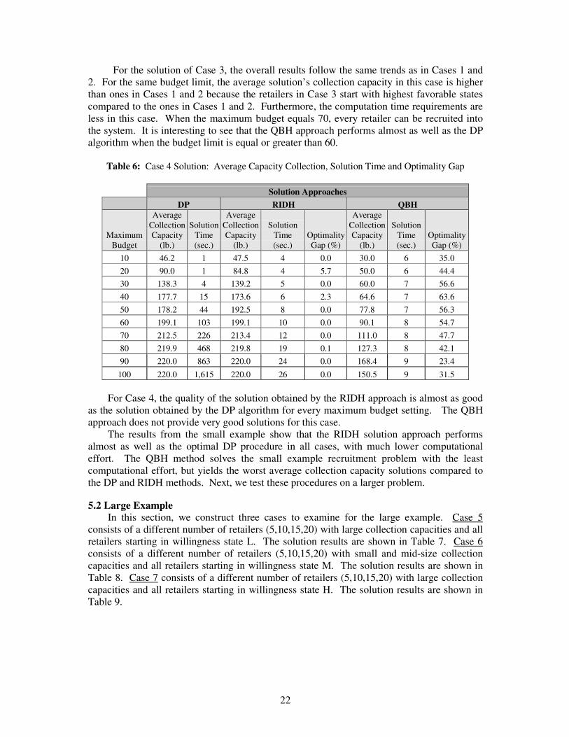
For the solution of Case 3, the overall results follow the same trends as in Cases 1 and 2. For the same budget limit, the average solution’s collection capacity in this case is higher than ones in Cases 1 and 2 because the retailers in Case 3 start with highest favorable states compared to the ones in Cases 1 and 2. Furthermore, the computation time requirements are less in this case. When the maximum budget equals 70, every retailer can be recruited into the system. It is interesting to see that the QBH approach performs almost as well as the DP algorithm when the budget limit is equal or greater than 60.


Solution Approaches DP RIDH QBH

Maximum Budget


(lb.)



(lb.)


Optimality Gap (%)


(lb.)


Optimality Gap (%)

10 46.2 1 47.5 4 0.0 30.0 6 35.0 20 90.0 1 84.8 4 5.7 50.0 6 44.4 30 138.3 4 139.2 5 0.0 60.0 7 56.6 40 177.7 15 173.6 6 2.3 64.6 7 63.6 50 178.2 44 192.5 8 0.0 77.8 7 56.3 60 199.1 103 199.1 10 0.0 90.1 8 54.7 70 212.5 226 213.4 12 0.0 111.0 8 47.7 80 219.9 468 219.8 19 0.1 127.3 8 42.1 90 220.0 863 220.0 24 0.0 168.4 9 23.4

100 220.0 1,615 220.0 26 0.0 150.5 9 31.5 For Case 4, the quality of the solution obtained by the RIDH approach is almost as good

as the solution obtained by the DP algorithm for every maximum budget setting. The QBH approach does not provide very good solutions for this case.

The results from the small example show that the RIDH solution approach performs almost as well as the optimal DP procedure in all cases, with much lower computational effort. The QBH method solves the small example recruitment problem with the least computational effort, but yields the worst average collection capacity solutions compared to the DP and RIDH methods. Next, we test these procedures on a larger problem.

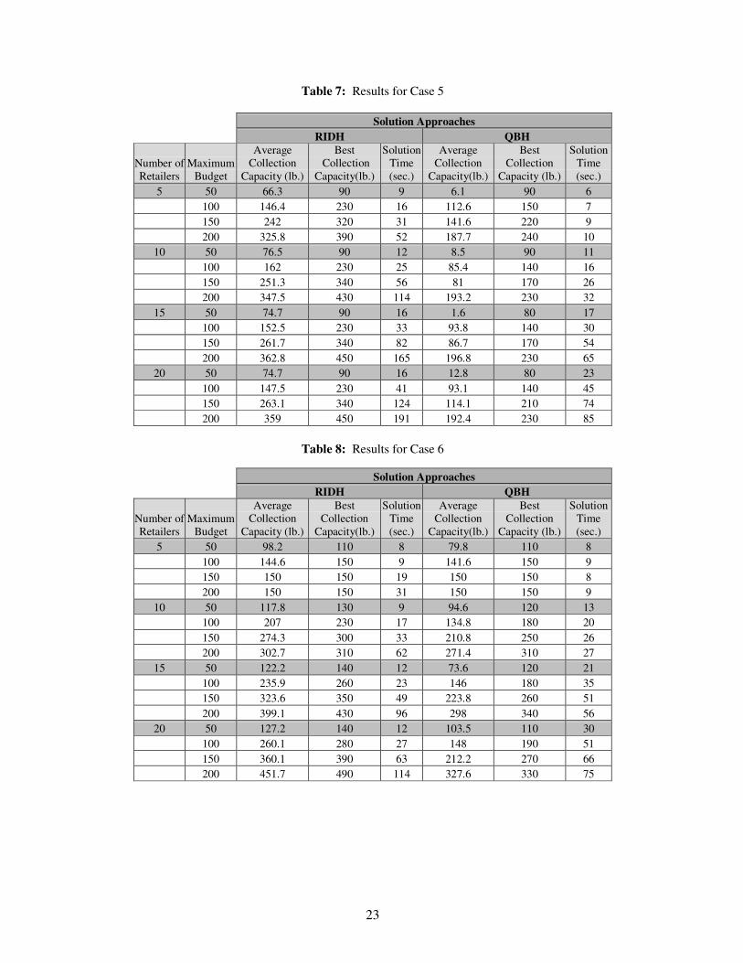
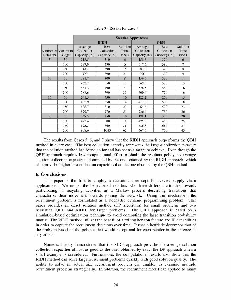
5.2 Large Example In this section, we construct three cases to examine for the large example. Case 5

consists of a different number of retailers (5,10,15,20) with large collection capacities and all retailers starting in willingness state L. The solution results are shown in Table 7. Case 6 consists of a different number of retailers (5,10,15,20) with small and mid-size collection capacities and all retailers starting in willingness state M. The solution results are shown in Table 8. Case 7 consists of a different number of retailers (5,10,15,20) with large collection capacities and all retailers starting in willingness state H. The solution results are shown in Table 9.

23

Table 7: Results for Case 5

Solution Approaches RIDH QBH

Number of Retailers

Maximum Budget

Average Collection

Capacity (lb.)

Best Collection

Capacity(lb.)


Average Collection

Capacity(lb.)

Best Collection

Capacity (lb.)


5 50 66.3 90 9 6.1 90 6 100 146.4 230 16 112.6 150 7 150 242 320 31 141.6 220 9 200 325.8 390 52 187.7 240 10

10 50 76.5 90 12 8.5 90 11 100 162 230 25 85.4 140 16 150 251.3 340 56 81 170 26 200 347.5 430 114 193.2 230 32

15 50 74.7 90 16 1.6 80 17 100 152.5 230 33 93.8 140 30 150 261.7 340 82 86.7 170 54 200 362.8 450 165 196.8 230 65

20 50 74.7 90 16 12.8 80 23 100 147.5 230 41 93.1 140 45 150 263.1 340 124 114.1 210 74 200 359 450 191 192.4 230 85



Number of Retailers

Maximum Budget

Average Collection

Capacity (lb.)

Best Collection

Capacity(lb.)


Average Collection

Capacity(lb.)

Best Collection

Capacity (lb.)


5 50 98.2 110 8 79.8 110 8 100 144.6 150 9 141.6 150 9 150 150 150 19 150 150 8 200 150 150 31 150 150 9

10 50 117.8 130 9 94.6 120 13 100 207 230 17 134.8 180 20 150 274.3 300 33 210.8 250 26 200 302.7 310 62 271.4 310 27

15 50 122.2 140 12 73.6 120 21 100 235.9 260 23 146 180 35 150 323.6 350 49 223.8 260 51 200 399.1 430 96 298 340 56

20 50 127.2 140 12 103.5 110 30 100 260.1 280 27 148 190 51 150 360.1 390 63 212.2 270 66 200 451.7 490 114 327.6 330 75

24



Number of Retailers

Maximum Budget

Average Collection

Capacity (lb.)

Best Collection

Capacity(lb.)


Average Collection

Capacity(lb.)

Best Collection

Capacity (lb.)


5 50 218.5 310 6 155.6 320 6 100 387.9 390 6 317.5 390 7 150 390 390 15 381.6 390 9 200 390 390 21 390 390 9

10 50 231.7 300 8 156.6 330 11 100 462.7 550 11 349.3 530 13 150 661.3 790 21 528.5 560 16 200 788.6 790 33 600.4 720 16

15 50 241.5 350 10 122.2 250 15 100 465.9 550 14 412.3 500 18 150 688.7 810 27 464.6 570 23 200 879.7 970 51 736.4 790 26

20 50 248.5 350 10 188.1 320 20 100 473.4 600 18 425.6 480 25 150 695.3 860 36 586.8 680 37 200 908.6 1040 62 667.3 760 43

The results from Cases 5, 6, and 7 show that the RIDH approach outperforms the QBH

method in every case. The best collection capacity represents the largest collection capacity that the solution method has found so far and has set as a target to achieve. Even though the QBH approach requires less computational effort to obtain the resultant policy, its average solution collection capacity is dominated by the one obtained by the RIDH approach, which also provides higher best collection capacities than the one obtained by the QBH method.

6. Conclusions This paper is the first to employ a recruitment concept for reverse supply chain

applications. We model the behavior of retailers who have different attitudes towards participating in recycling activities as a Markov process describing transitions that characterize their movement towards joining the network. Using this mechanism, the recruitment problem is formulated as a stochastic dynamic programming problem. This paper provides an exact solution method (DP algorithm) for small problems and two heuristics, QBH and RIDH, for larger problems. The QBH approach is based on a simulation-based optimization technique to avoid computing the large transition probability matrix. The RIDH method utilizes the benefit of a rolling horizon feature and IP capabilities in order to capture the recruitment decisions over time. It uses a heuristic decomposition of the problem based on the policies that would be optimal for each retailer in the absence of any others.

Numerical study demonstrates that the RIDH approach provides the average solution

collection capacities almost as good as the ones obtained by exact the DP approach when a small example is considered. Furthermore, the computational results also show that the RIDH method can solve large recruitment problems quickly with good solution quality. The ability to solve an actual size recruitment problem can enables us examine multiple recruitment problems strategically. In addition, the recruitment model can applied to many

25

types of recruitment problems such as recruiting supermarket stores for the collection of plastic bottles in the plastic recycling industry and recruiting the major electronic stores such as Best Buy and Circuit City for used electronics equipment in the electronic scrap recycling industry. If these decisions were left up to individual store managers and not centrally mandated.

Results from this paper raise new questions and several potential directions of future research. Future extensions can be envisioned in both the modeling and solution methodology areas.

Currently we have developed a tactical collection model under the assumption that once the agent is recruited to the network, it always stays in the network. However, in actual situations, sometimes a collection agent may opt to leave the network. Future work includes extending the recruitment model to include retention and defection considerations. An important subtask is to define the criteria that determine the retention and defection actions of the agent after it is recruited. The additional complexity will impact the capability of the current approach to solve large scale collection recruitment problems. Another direction of future work includes exploring the collection logistics where the generation rate of collection material is stochastic among the agents. With this uncertainty, the problem of routing a fixed number of finite capacity trucks to collect the material from the collection agents is more difficult.

In addition, in the real application, the recruitment process and retailer retention may depend not only on the connection between the retailers and the recruiter, but also on the outside market, a competitor. For example, currently companies in China are showing interest in used carpet from U.S. sources to bring it to China for recycling. Hence, there can be a competition for the desired source. Retailers both in and out of the collection network may opt to give the source to competitor collectors who provide a better incentive. This also affects the recruitment allocation plan for the carpet recycler in the U.S. Adding a competition feature from the game theory perspective to the recruitment model can complicate the model framework but provides a deeper understanding of how the entities might act in the real situation.

References Adelman, D. and Mersereau, A.J. (2004), “Relaxations of Weakly Coupled Stochastic

Dynamic Programs,” Working Paper, Graduate School of Business, The University of Chicago

Bass, F. (1969), “A New Product Growth Model for Consumer Durables,” Management Science, 15(1), 215-227.

Bertsimas, D. and Nino-Mora, J. (2000), “Restless Bandits, Linear Programming Relaxations, and a Primal-Dual Index Heuristic,” Operations Research, 48(1), 80-90.

Bellman, R.E. (1957), Dynamic Programming, Princeton University Press, Princeton, New Jersey, USA.

Canada's Waste Recycling Marketplace (2006), http://www.recyclexchange.com, viewed 03/16/2006.

Carpet America Recovery Effort (2004), “Carpet America Recovery Effort’s Annual Report in 2004,” http://www.carpetrecovery.org/annual_report/04_CARE-annual-rpt.pdf, viewed 03/16/2006.

Coughlan, A.T., Grayson, K. (1998), “Network Marketing Organizations: Compensation Plans, Retail Network Growth, and Profitability,” International Journal of Research in Marketing, 15, 401-426.

26

Darmon, R. Y. (2003), “Controlling Sales Force Turnover Costs though Optimal Recruiting and Training Policies,” European Journal of Operation Research, 154, 291-303.

Gosavi, A. (2003), Simulation-based Optimization: Parametric Optimization Techniques and Reinforcement Learning, Kluwer Academic Publishers.

Georgiou, A.C., Tsantas, N. (2002), “Modeling Recruiting Training in Mathematical Human Resource Planning,” Applied Stochastic Models in Business and Industry, 18, 53-74.

Hawkins, D.A. (1992), “An Activation-recruitment Scheme for Use in Muscle Modeling,” Journal of Biomechanics, 25, 1467-1476.

IDES The Plastics Web (2006),http://www.ides.com/resinprice/resinpricingreport.asp, viewed 03/16/2006.

Kaelbling, L.P., Littman, M.L., Moore, A.W. (1996), “Reinforcement Learning: A Survey,” Journal of Artificial Intelligence Research, 4, 237-285.

Knuth, D. (1973), The Art of Computer Programming, Volume 3: Sorting and Searching, Addison Wesley.

Mehlmann, A. (1980), “An approach to optimal recruitment and transition strategies for manpower systems using dynamic programming,” Journal of the Operational Research Society, 31, 1009-1015.

Puterman, M.L. (1994), Markov Decision Processes, Wiley Interscience, New York, USA. Seggern, V.D. (1993), CRC Standard Curves and Surfaces. Boca Raton, FL: CRC Press, p.

124, 1993. Treven, S. (2006), “Human Resources Management in the Global Environment,” Journal

of American Academy of Business, 8, 120-125. Watkins, C.J. (1989), “Learning from Delayed Rewards,” Ph.D. Dissertation, Kings College,

Cambridge, England, May 1989. Whittle, P. (1988), “ Restless Bandits: Activity Allocation in a Changing World,” J. Gani,

ed. A Celebration of Applied Probability, Journal of Applied Probability, 25A, 287-298.

Documents

226 recruiting suppliers for reverse production systems.doc) - Optimization … · · 2007-03-14Recruiting Suppliers for Reverse Production Systems: an MDP Heuristics Approach Wuthichai