2265 116th Avenue N.E., Bellevue, WA 98004 Finance and ... · PDF fileFinance and Administration: (425) 453-9489 Fax: (425) 453-3199 ... Sensors detect physical phenomena and ... Several

2265 116th Avenue N.E., Bellevue, WA 98004 Sales and Customer Support: (425) 453-2345

Finance and Administration: (425) 453-9489 Fax: (425) 453-3199

WWW: http://www.mstarlabs.com/

From the Microstar Laboratories web site

Temperature Measurement Temperature Measurements using Data Acquisition Processors Off-the-shelf temperature measurement and display products are excellent for what they do. They offer accuracy within a couple of percent, sometimes better. And they are ready to go with all necessary functions included. If they do what you want, you should use them. But if they don't have exactly what you need, they offer you few options. See how Data Acquisition Processors can help.

Take a look at some sample multi-channel system drawings. DAP 4000a System | DAP 5200a System | DAP 5216a System

Choosing Sensors

Sensors detect physical phenomena and convert these to corresponding electrical signals that are relatively easy to measure. Sensors that do not produce an electrical signal naturally are supplemented with electronics to produce the measurable signal.

Several temperature sensor types are available, each with its own strengths and weaknesses. To help you make an appropriate selection, here are brief descriptions of some of the most important temperature sensor types. DAPs are intended to work with any sort of sensor that delivers a measurable electrical signal.

www.mstarlabs.com/sensors/temperature.html Page 1

http://www.mstarlabs.com/

http://www.mstarlabs.com/dataacquisition/graphics/dap4000adrawing.html



Calibration

The term calibration is often used incorrectly, to mean applying a standardized device curve. That assumes that a real device will conform perfectly to the selected theoretical curve. In practice, any real device will deviate from published theoretical curves, which are only statistical composites. A true calibration process determines how an actual device responds, given inputs established by a reference standard.

Published standard curves are a good start, and sensor manufacturers try to match them as close as they can, but actual devices deviate from the ideal. Check your tolerance requirements. If you don't need best accuracy, keep things simple, and stay with "typical" curves. But for better accuracy, calibrate. Check the calibration and linearization page for more information.

Some DAPL processing commands can help you apply sensor calibration for improved measurement accuracy.

• The INTERP command can represent nonlinear response curves of arbitrary sensor devices over an extended range.

• The RTD command can apply nominal or calibrated conversion curves for RTD devices.

• The THERMISTOR command can apply nominal or calibrated conversion curves for thermistor devices.

Measurement

Temperature sensors tend to fall into two categories: those that produce a voltage naturally as an indicator of temperature, and those that produce some other physical response that must be converted to a voltage for measurement.

• Natural output potentials.

The signals may be weak or strong. When weak, they are vulnerable to external interference. When strong, they typically require a power source to drive them, with potential dangers of power supply noise leaking into the measurements. For both cases, differential signals help to keep the measurements clean.

When working with natural voltages, you will typically need:

ThermocoupleExample

RTD Example

ThermistorExample


http://www.mstarlabs.com/software/dapl/commands.html

• A SCALE or DAPL expression command to correct for gains and offsets.

• A linearization command like THERMO or INTERP to compensate for nonlinearity and calculate the corresponding temperature.

The article Thermocouple Measurement Applications on this site describes a low-cost, low-speed 8 channel application using thermocouples. It applies averaging for noise reduction, a conventional cold junction compensation device, and standard conversion curves for measurements of moderate accuracy.

Another article on this site covers accurate measurement withthermocouples, using carefully-calibrated measurements and coldjunction compensation.

• Indirect voltage output.

Excitation power is typically required to convert the response into anelectrical signal.

For example, resistive devices are driven by regulated voltage or current sources. You will typically need:

• A SCALE or DAPL expression command to correct for gains and offsets.

• A command like DIVIDER or BRIDGE to determine the device resistance from observed output voltage.

• A command like RTD or THERMISTOR to convert from a resistance measurement to the corresponding operating temperature.

An article on this site describes an application using a thermistor in conjuction with a thermocouple, for very accurate measurements of cold junction temperature.

Another article on this site discusses an application using an RTD for measuring moderately high temperatures with moderate accuracy, using simple calibration procedures.


http://www.mstarlabs.com/apeng/integration/thermapp.html

Better Temperature Measurements for Systems Temperature Measurements: More, Better, Faster Here are some of the difficult temperature measurement problems Data Acquisition Processor (DAP) boards can help with.

Cost | Packaging | Display | Integration | Diversity | Accuracy | Speed | Noise

COSTS

Problem: Fully integrated measurement devices are high cost per channel.

Data Acquisition Processors have a higher initial cost, but then a much lower cost per channel, which turns into an economic advantage when you have lots of channels. The cost of adding a channel is roughly the cost of the extra wiring and sensor.

PACKAGING

Problem: Independently packaged measurement devices can fill a rack in a hurry.

Adding channels to a Data Acquisition Processor system requires only the additional panel space for your connectors.

DISPLAY

Problem: The built-in display that is a strong advantage for a single signal becomes a disadvantage when you have lots of channels.

Data Acquisition Processors can deliver the data for display in any manner that you wish, including software-controlled video graphics of your choosing.

INTEGRATION

Problem: Self-contained units offer limited options for interconnection.

Data Acquisition Processors bring measurements directly into your host system on a high-speed data bus. From there, you can apply the data management and networking features of your host system to send data anywhere.


http://www.mstarlabs.com/dataacquisition/dap.html

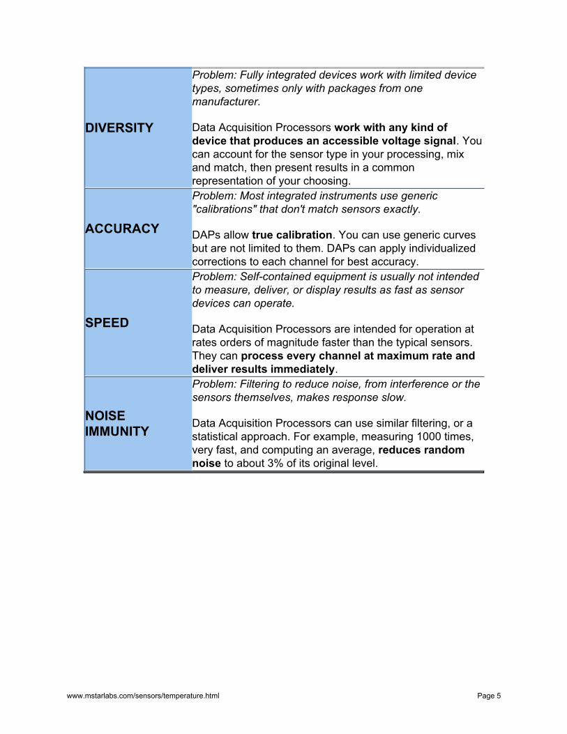
DIVERSITY

Problem: Fully integrated devices work with limited device types, sometimes only with packages from one manufacturer.

Data Acquisition Processors work with any kind of device that produces an accessible voltage signal. You can account for the sensor type in your processing, mix and match, then present results in a common representation of your choosing.

ACCURACY

Problem: Most integrated instruments use generic "calibrations" that don't match sensors exactly.

DAPs allow true calibration. You can use generic curves but are not limited to them. DAPs can apply individualized corrections to each channel for best accuracy.

SPEED

Problem: Self-contained equipment is usually not intended to measure, deliver, or display results as fast as sensor devices can operate.

Data Acquisition Processors are intended for operation at rates orders of magnitude faster than the typical sensors. They can process every channel at maximum rate and deliver results immediately.

NOISE IMMUNITY

Problem: Filtering to reduce noise, from interference or the sensors themselves, makes response slow.

Data Acquisition Processors can use similar filtering, or a statistical approach. For example, measuring 1000 times, very fast, and computing an average, reduces random noise to about 3% of its original level.


Temperature Sensors Survey Common Temperature Measurement Sensors This page surveys the most common temperature measurement sensor types.

Thermocouples | RTDs | Thermistors | Infrared | Solid State | Bimetallic

Thermocouple

These sensors depend on differences in charge mobility in two dissimilar metals to produce a potential difference. The developed potentials are small, but measurable.

Thermocouples are rugged, and tolerate a wide range of temperatures, but they have many drawbacks, including low signal levels, long-term stability, and noise. Their response time tends to be very slow, but this often results from the packaging more than the device physics.

The measurement is actually temperature difference, not an absolute temperature level, so a supplementary measurement is required to establish the reference temperature. The resulting temperature correction is called cold junction compensation.

Despite their limitations, thermocouples are used with success

ThermocoupleExample

ThermocoupleCalibration

Cold JunctionCompensation

in a variety of applications. You can obtain moderate accuracy using standard device curves with no calibration. Careful calibration can improve accuracy to within a degree C or so.


http://www.mstarlabs.com/sensors/thermocouple-calibration.html

http://www.mstarlabs.com/sensors/thermocouple-cold-junctions.html


RTD

RTDs, short for "resistive thermal devices," are built basically the same way as wire-wound or thin-film resistors, but using materials with relatively high levels of resistivity variation as a function of temperature. They are generally between thermocouples and thermistors in terms of speed, ruggedness, signal level and temperature range.

If not severely stressed, they have good long term stability.

They cost more, but offer superior linearity and good accuracy

RTD Example

RTD Calibration

using standard curves without calibration. With individual device calibration, the accuracy is even better.

Though most common metals exhibit RTD effects, platinum alloys have the best range and performance, and are by far the most popular.

Thermistor

Negative temperature coefficient thermistors, the ones commonly used for temperature measurements, change resistance dramatically in response to temperature changes, but they have some limitations.

They are vulnerable to physical damage and chemical contamination — for example, water can cause problems. They require careful protective packaging, and this often limits how they can be used. Response is moderately fast, but typically limited because of the packaging. The thermal characteristics are highly nonlinear, so you must apply corrections that differ for every device type. For full accuracy you must calibrate. They have a limited range compared to other thermal sensors.

ThermistorExample

ThermistorCalibration

For the temperatures where liquid water can exist, thermistors usually perform very well.

Infrared

These sensors include special optical and electrical components to detect infrared blackbody radiation from a very specific location, without direct physical contact.


These sensors are very useful for measuring extreme temperatures through a viewing port, under conditions that would rapidly destroy other sensor types.

The accuracy, stability, and repeatability are not very good, so they need a lot of attention.

The receiver/converter electronics scale the signal to convenient levels for acquisition and recording.

Solid state

These devices use the thermal properties of semiconductor junction voltages to detect temperature.

These devices are appealing because sensor, power-gain amplifiers, and "linearization" can be fabricated on the same chip.

The drawbacks are that the operating range of the electronics limits the sensing range, and any calibration other than offset adjustment is impractical.

These are extremely handy for measuring ambient temperatures around circuit boards, and popular for "cold junction compensation" in combination with thermocouples. Accuracy is moderate.

Bimetallic

We mention this one only in passing. A sensor bonded to a bimetallic strip senses strain in proportion to temperature changes. This is too bulky, slow, and vulnerable to mechanical and electrical interference for most applications, but compatible.


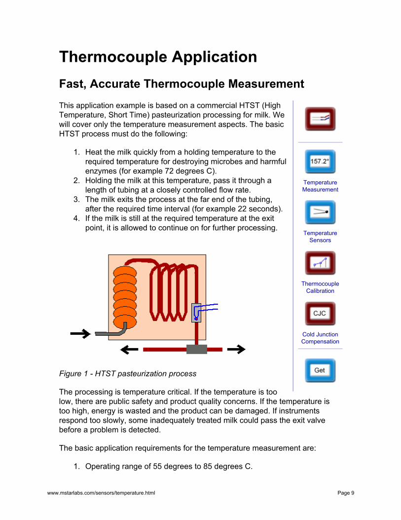
Thermocouple Application Fast, Accurate Thermocouple Measurement This application example is based on a commercial HTST (High Temperature, Short Time) pasteurization processing for milk. We will cover only the temperature measurement aspects. The basic HTST process must do the following:

1. Heat the milk quickly from a holding temperature to the required temperature for destroying microbes and harmful enzymes (for example 72 degrees C).

2. Holding the milk at this temperature, pass it through a length of tubing at a closely controlled flow rate.

3. The milk exits the process at the far end of the tubing, after the required time interval (for example 22 seconds).

4. If the milk is still at the required temperature at the exit point, it is allowed to continue on for further processing.

Figure 1 - HTST pasteurization process

The processing is temperature critical. If the temperature is too

TemperatureMeasurement

TemperatureSensors



low, there are public safety and product quality concerns. If the temperature is too high, energy is wasted and the product can be damaged. If instruments respond too slowly, some inadequately treated milk could pass the exit valve before a problem is detected.

The basic application requirements for the temperature measurement are:

1. Operating range of 55 degrees to 85 degrees C.


http://www.mstarlabs.com/sensors/download-commands.html

2. No physical damage from out-of-range temperatures. 3. Total measurement accuracy +- 0.5 degrees C. 4. Long term drift +- 0.2 degrees C. 5. Maximum settling time 4 seconds.

Selecting a sensor A high quality type T thermocouple probe is selected. Thermistors have good response characteristics but are vulnerable to moisture and damage. RTDs have better stability and linearity, but slow response times — perhaps this is because the entire RTD has to settle to thermal equilibrium before a reading is accurate, whereas only a thermocouple probe tip needs to settle to temperature.

High quality type T thermocouple probes can be calibrated to an accuracy of about 0.1 degrees C. These use very fine gage wires that can reach a thermal equilibrium quickly. To prevent chemical interaction with the milk products there must be a protective cover. This will degrade the thermal response rate significantly, but if the resulting time constant remains under 0.5 seconds, the settling time requirement is met easily.

The main challenge with a thermocouple sensor is the very low signal level, difficult to isolate from background noise.

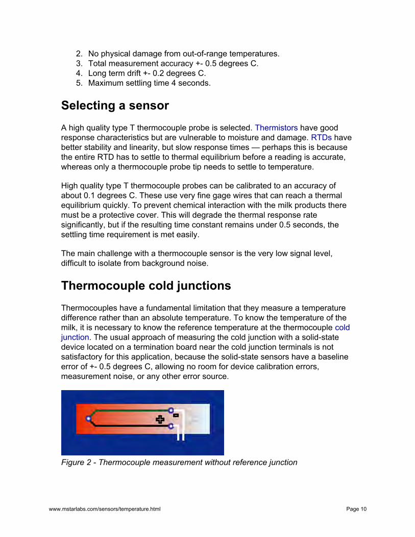
Thermocouple cold junctions Thermocouples have a fundamental limitation that they measure a temperature difference rather than an absolute temperature. To know the temperature of the milk, it is necessary to know the reference temperature at the thermocouple cold junction. The usual approach of measuring the cold junction with a solid-state device located on a termination board near the cold junction terminals is not satisfactory for this application, because the solid-state sensors have a baseline error of +- 0.5 degrees C, allowing no room for device calibration errors, measurement noise, or any other error source.

Figure 2 - Thermocouple measurement without reference junction



The issue of how to obtain an accurate cold junction measurement is covered in a separate note. We will merely presume here that there is a separate temperature measurement involved, and that the cold junction absolute temperature is known within +- 0.1 degrees C.

Signal conditioning and sampling An MSXB065 differential signal conditioning and filtering board amplifies the low-level thermocouple signal, applying a gain of 25 and raising the signal range to approximately 0.1 volts. Despite best efforts to shield the signals from noise, some interfering noise will leak in and add to the inherently noisy readings from the thermocouple. A fourth order Butterworth filter tuned to a 500 Hz cutoff will remove all high frequency random noise from the measurements.

Applications with less stringent accuracy and speed requirements can route thermocouples directly to a termination board, with an onboard CJC circuit, and breadboarding space for termination networks.

The excitation and signal lines required for the thermocouple and supplementary cold junction sensors are provided through the 37-in panel connector of the MSXB 065. A balanced termination network on the board provides a ground reference voltage so that the thermocouple junction does not "float" to a high common mode voltage.

We will choose a DAP 5000a for the sampling and data processing. A DAP 5000a provides good support for numerical filtering operations, plus processing capacity for additional monitoring functions not covered here.

With less stringent measurement requirements, you would probably choose a DAP 840.

Figure 3 - MSXB 065 signal conditioning board

Figure 4 - DAP 5000a board


http://www.mstarlabs.com/access/xb065.html


http://www.mstarlabs.com/access/termination.html

http://www.mstarlabs.com/dataacquisition/dap5000a.html


http://www.mstarlabs.com/dataacquisition/840/840spec.html

For supporting more channels and more complex calibration curves, you would probably choose a DAP 5200a.

The 100 millivolt signal level is still too small to digitize with good precision. Configure the input sampling of the Data Acquisition Processor to apply an additional gain of 40. This will raise the signal range to about 4 volts, within the usual +/- 5 volt input range used by most Data Acquisition Processor configurations. In the input configuration, your input channel definition will look something like the following:

SET IP1 D1 40

Over the temperature range of 55 degrees to 85 degrees, the response levels of the thermocouple range from 2.251 to 3.385 millivolts, so the range of variations seen by the converters are 2.251 to 3.385 volts. This is 1.134 volts out of the full 10 volt span — 1858 converter counts out of the 16384 counts available with a 14-bit converter. That gives a temperature resolution of 30/1858 = 0.02 degrees. If we presume that the last two bits of the converter are compromised by converter chatter and nonlinearity, that still yields measurement accuracy better than 0.08 degrees C.

Processing and digital filtering Sampling at 1500 samples per second guarantees that any signal passing through the 500 Hz lowpass filter is accurately represented, including lower-frequency noise. We can use the following command to smooth the signal and reduce the sampling rate to a more friendly 150 samples per second for processing.

FIRLOWPASS(IP1, 10, PREDUCED)

After filtering, all noise beyond 75% of the Nyquist frequency (75 samples per second x 0.75) are gone. In particular, all 60 Hz interference from power sources is gone.

The 150 samples per second can still exhibit residual random noise in the 10 to 50 Hz range. We can apply digital filtering to remove most of that, with care. The lower the cutoff frequency, the more time delay in producing results. The 10 Hz cutoff is selected to keep this filtering delay relatively small. We can apply a 4th order inverse Chebyshev filter with 46 dB stopband rejection to remove the higher frequencies sharply while preserving the low-frequency temperature variations accurately. 10 Hz is 0.1333 of the Nyquist frequency of 75 Hz, so we specify the following digital filter.



http://www.mstarlabs.com/software/dapl/dapl-dsp-filtering.html

CHEBYINV(PREDUCED, 4, 0.1333, 0.005, PFILT)

Calibration and conversions The data stream PFILT above will have clean measurements of thermocouple junction potential, but these results must be converted into the desired temperature measurements. We know that for a precision type-T thermocouple, the response is almost linear in the limited operating range. If we measure the thermocouple's output potential at the limits of the operating range (55 degrees and 85 degrees C, call these measured values POT55 and POT85), the following DAPL expression can convert the measured junction potential to the corresponding temperature anywhere in the range.

LINTEMP = \((POT85-PFILT)*55.0 + (PFILT-POT55)*85.0)) \/ (POT85-POT55)

The measurements used for the calibration include any effects from offsets and gain DAPL expressions look like deviations in the amplifiers. So in additional to simple arithmetic — but accounting for the thermocouple response, they actually define the calibration above also covers the complete processing tasks measurement hardware. The usual approach that apply conversion of applying standard curves does not take operations to your entire measurement errors and sensor variations data stream. Learn more. into account.

Unfortunately, the simple linear mapping as described above isn't completely satisfactory. From the standard type-T characteristic curve, we can learn that there is a maximum deviation of about -0.20 degrees from a linear curve in this range. We can easily correct for this effect, using an additional DAPL expression.

TADJUSTED = LINTEMP + ( -0.20 * 4.0 * \(PFILT-POT55)/(POT85-POT55) * \(POT85-PFILT)/(POT85-POT55) )

You can verify that the second-order correction is zero at the ends of the ranges, and equal to the maximum -0.20 at the center of the range. The residual error in the corrected temperature reading is just a few hundredths of a degree. Thus, conversion errors are almost insignificant. Total system error depends almost exclusively on the quality of the signal and calibration.

The final temperature measurements are available 150 times per second, with a delay of a few milliseconds after receiving each temperature update. Total


http://www.mstarlabs.com/software/dapl/tabs.html

response delay depends almost exclusively on the temperature probe time constant.

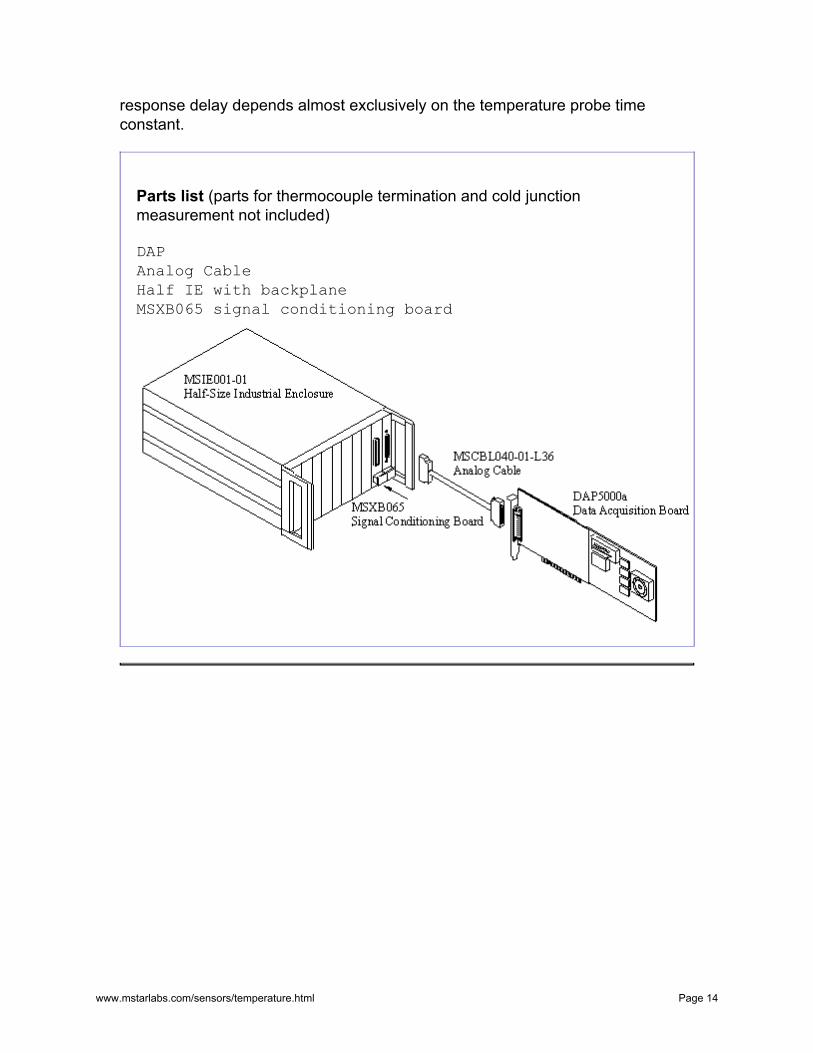
Parts list (parts for thermocouple termination and cold junction measurement not included)

DAP Analog CableHalf IE with backplaneMSXB065 signal conditioning board


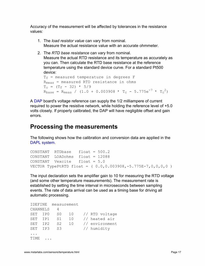
RTD Application RTD Measurements for Roaster Control Producing a rich, aromatic cup of java requires a blend of art, science, and good coffee beans. A critical step is the roasting of the beans. There are hundreds of complex organic chemicals that produce the flavors and aromas. Roasting brings out some of these, and produces others, in a manner highly dependent on timing and temperatures. Good roasting techniques can produce quite acceptable results from relatively low-grade beans; bad roasting can produce quite dreadful results from the best high-grade beans.

Profile roasting Green coffee beans are placed into a drum or chamber, where they are agitated or tumbled as they are roasted by hot air. There are four controllable variables:

1. temperature of the hot air 2. air flow rate 3. temperature of the beans 4. stir rate

The most successful and repeatable control strategy is called profile control. Rather than trying to hold specific temperatures, the temperature targets are treated as a continuously changing trajectory. The amount of heating at "each level" depends on the rates of temperature change.

Temperature sensing


TemperatureSensors

RTD Calibration

The critical variable is the temperature of the beans. Other variables can help to improve the control of the critical variable. The heated air is easier to measure, but it can differ from the bean temperature by as much as 200 degrees F, so it is not a sufficient indicator by itself.

A thermal probe measuring the temperature within the coffee beans provides the most important feedback. The probe must withstand the pounding as beans are tumbled. Because of its rugged sheath, this kind of probe will not respond



quickly, but the temperature profile will not change very fast either, and a reasonable balance is maintained.

Either a thermocouple or RTD probe could work for this application. We will select an RTD probe because it is reliable, accurate, stable, easy to use, and well suited for an operating temperature range of 100 to 500 degrees F.

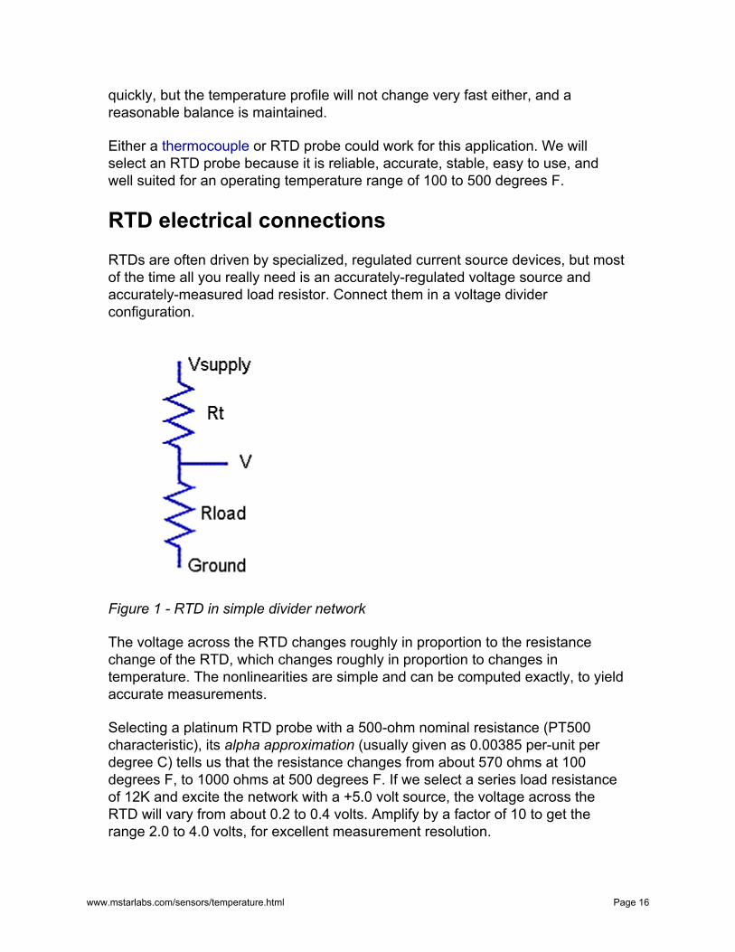
RTD electrical connections RTDs are often driven by specialized, regulated current source devices, but most of the time all you really need is an accurately-regulated voltage source and accurately-measured load resistor. Connect them in a voltage divider configuration.

Figure 1 - RTD in simple divider network

The voltage across the RTD changes roughly in proportion to the resistance change of the RTD, which changes roughly in proportion to changes in temperature. The nonlinearities are simple and can be computed exactly, to yield accurate measurements.

Selecting a platinum RTD probe with a 500-ohm nominal resistance (PT500 characteristic), its alpha approximation (usually given as 0.00385 per-unit per degree C) tells us that the resistance changes from about 570 ohms at 100 degrees F, to 1000 ohms at 500 degrees F. If we select a series load resistance of 12K and excite the network with a +5.0 volt source, the voltage across the RTD will vary from about 0.2 to 0.4 volts. Amplify by a factor of 10 to get the range 2.0 to 4.0 volts, for excellent measurement resolution.


Accuracy of the measurement will be affected by tolerances in the resistance values:

1. The load resistor value can vary from nominal.Measure the actual resistance value with an accurate ohmmeter.

2. The RTD base resistance can vary from nominal. Measure the actual RTD resistance and its temperature as accurately as you can. Then calculate the RTD base resistance at the reference temperature using the standard device curve. For a standard Pt500 device: Tf = measured temperature in degrees FRmeas = measured RTD resistance in ohmsTc = (Tf - 32) * 5/9

2)Rbase = Rmeas / (1.0 + 0.003908 * Tc - 5.775e-7 * Tc

A DAP board's voltage reference can supply the 1/2 milliampere of current required to power the resistive network, while holding the reference level of +5.0 volts closely. If properly calibrated, the DAP will have negligible offset and gain errors.

Processing the measurements The following shows how the calibration and conversion data are applied in the DAPL system.

CONSTANT RTDbase float = 500.2CONSTANT LOADohms float = 12088CONSTANT Vexcite float = 5.0VECTOR TypePtRTD float = ( 0.0,0.003908,-5.775E-7,0,0,0,0 )

The input declaration sets the amplifier gain to 10 for measuring the RTD voltage (and some other temperature measurements). The measurement rate is established by setting the time interval in microseconds between sampling events. The rate of data arrival can be used as a timing base for driving all automatic processing.

IDEFINE measurementCHANNELS 4SET IP0 S0 10 // RTD voltageSET IP1 S1 10 // heated airSET IP2 S2 10 // environmentSET IP3 S3 // humidity...TIME ...




The processing includes commands that convert the captured voltage measurements into the corresponding temperature measurements. Two of these are DAPL expression tasks, and two are specialized downloadable commands available on this site.

PDEFINE processing// Correct for amplifier gainRTDvolts = IP0 / 10.0// Compute RTD resistanceDIVIDER( RTDvolts, LOADohms, Vexcite, RTDohms )// Convert RTD resistance to equivalent temperatureRTD( RTDohms, RTDbase, TypePtRTD, TEMPRdegc )// Convert temperature to FahrenheitTEMPRdegf = (9*TEMPRdegc/5)+32// Perform control algorithms here...// Select data for host displays here...END

More than just measurements Clearly, if monitoring one temperature were the complete story, a DAP system would provide more capability than you need. But an automated roasting process needs many other things to be successful. In addition to the basic measurements, DAPs can support the following:

• Supplementary measurement channels • Regulated sources • Trajectory generation • Device outputs • Interactive control algorithms • Local process monitoring • Remote data display and data logging

For supporting integrated measurement and control activity on multiple channels, the ability to incorporate RTD measurements along with other data capture and processing can be a real advantage. With most of the low-level details already covered, higher-level systems can concentrate on use interactions, profile configuration, and data management.


http://www.mstarlabs.com/software/dapl/commands.html


Thermistor Application Precise Measurement Using a Thermistor This page describes an application using an individually-calibrated thermistor to obtain highly accurate measurements of ambient temperature. This is an important side-problem for the HTST pasteurization application on this site: specifically, the temperature measurement of the thermocouple sensor used by that system does not completely determine the process temperature. The cold junction temperature must be measured accurately as well. Many of the application configuration issues are predetermined to satisfy the requirements of that system. Better than 0.1 degree C accuracy is required for the cold junction measurement in order to meet the stringent total measurement error requirements.

A sensor is needed that can measure absolute temperature with good stability and accuracy. Within the thermally protected environment where the thermocouple is terminated:

• Temperatures changes are small. • Temperatures changes occur very slowly. • The measuring device is subjected to minimal operating

stress.

This is a perfect place to take advantage of a thermistor's excellent responsiveness and accuracy.

Hardware details


TemperatureSensors


The pasteurization application uses an MSXB 065 signal conditioning and filtering board. The application reserves one of the channels on this board for cold junction measurements.

The MSXB065 and the thermocouple termination boards reside in an MSIE001 half-size standard rack enclosure. One slot is used by the interface board connecting the Data Acquisition Processor (DAP) board to the analog backplane. One slot is used by the MSXB 065. There is at least one slot for a thermal barrier, and then a slot used by a custom thermocouple termination board. The

The boards in the Channel Architecture conform to Eurocard formats, so you can easily obtain boards that fit within the enclosure and can meet EMC emissions standards.





http://www.mstarlabs.com/access/hwaccess.html

http://www.mstarlabs.com/access/hwaccess.html

http://www.mstarlabs.com/access/enclos.html


custom termination board provides a thermally stable environment, where the temperature can be measured accurately at the thermocouple cold junction terminals.

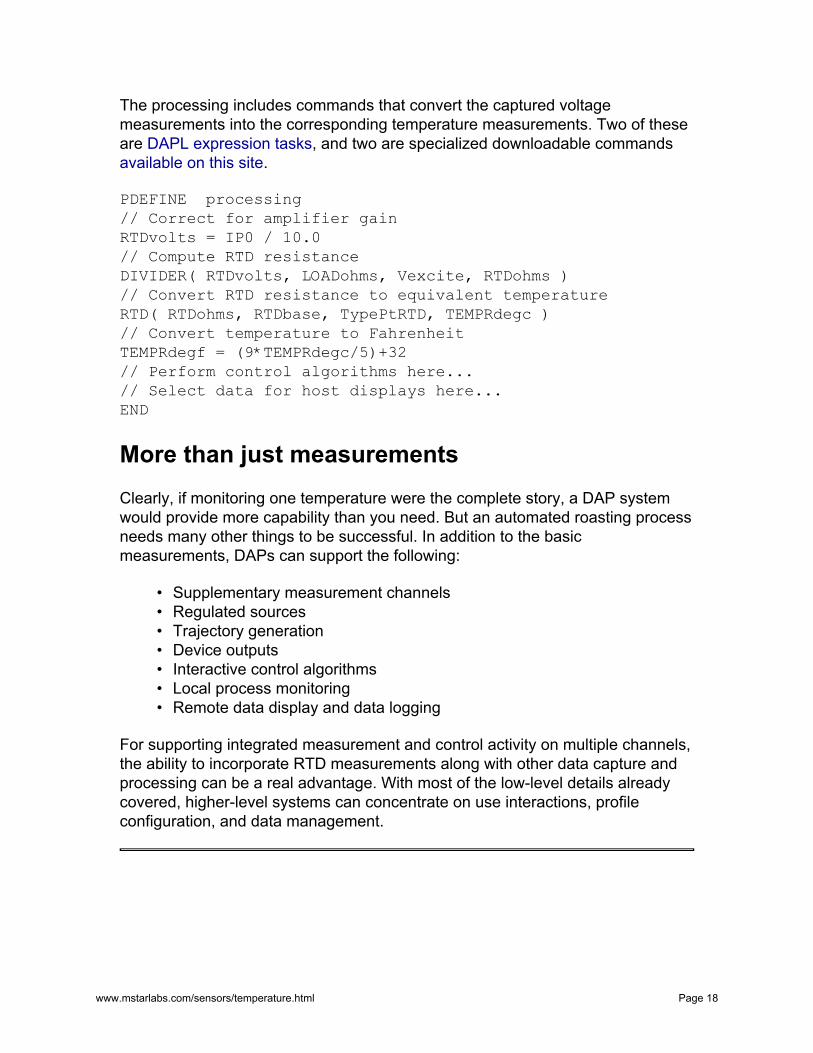
A cable must be built to connect the MSXB 065 to the thermocouple termination board.

Figure 1 - cable between boards

The thermocouple termination board is basically just a set of connectors. On the outside of the end panel, there are two connectors: a 37-pin D connector attaches to the signal conditioning board, and a thermocouple connector attaches to the thermocouple wires and their shield. On the inside, the board is blank and supports a terminal strip.

It is important for the thermistor to be mounted physically as close to the thermocouple wire termination as possible to avoid a temperature offset. One way to do this is to physically bond the thermistor body to the connector on the inside of the panel. Route the thermistor leads to connect at the terminal strip.

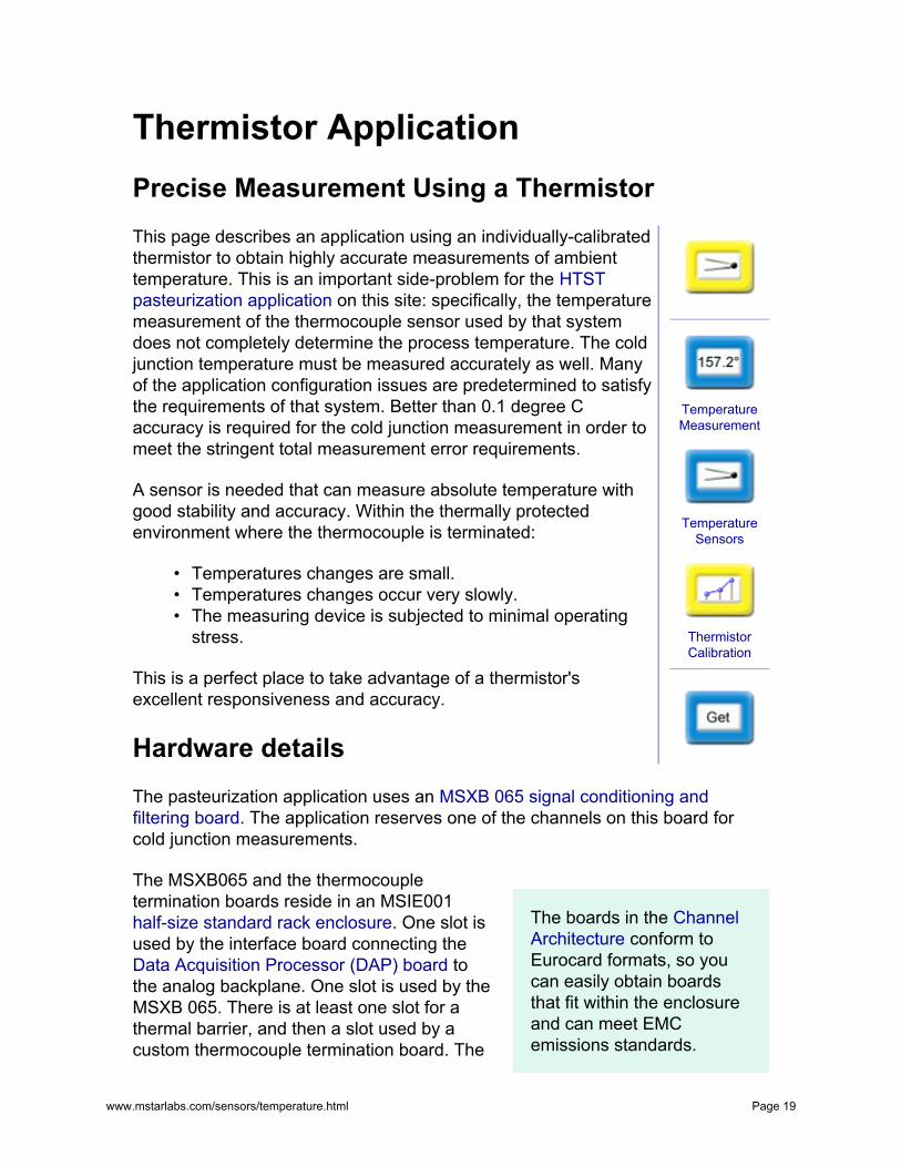
Beyond the point where the thermocouple wires terminate, use well-balanced conductors to connect to the terminal strip. On the other side of the terminal strip, connect to the excitation source and the differential measurement pins from the signal conditioning connector. The following diagram summarizes the electrical connections.


Figure 3 - thermistor connections on termination board

Thermistor characteristic calibration The MSXB065 board is configured for gains of 25 to detect very small thermocouple potentials. After applying the gain, the results must remain under +5 volts to be within the range of the Data Acquisition Processor. That means, 5/25 = 0.2 volts is a reasonable upper bound on the voltage across the thermistor when its resistance is maximum.

We pick a thermistor with a nominal value of about 1K at 25 degrees C. It happens to have a maximum value of about 2K in the operating range. To stay below 0.2 volts when the excitation voltage is +5 volts, we need a load resistor of about 50K. Choose standard value 56K for the loading resistor. Using a precision ohmmeter, determine the actual value. We will assume a measured value of 56.18K.

Assume an ambient temperature range 10 to 40 degrees C. The operating environment is unlikely to vary by this much, because milk must be refrigerated most of the time, and regulating the ambient temperature helps regulate the storage temperature. Even though this is a restricted range, the thermistor characteristic is nonlinear over this range and we need a correspondingly nonlinear characteristic to evaluate its response. See the thermistor calibration page for more information about how to do a simple three-point calibration. Here is the calibration data set. We will use the first, center, and last terms for an exact fit and evaluate the approximations at the other two points to check the interpolation accuracy.


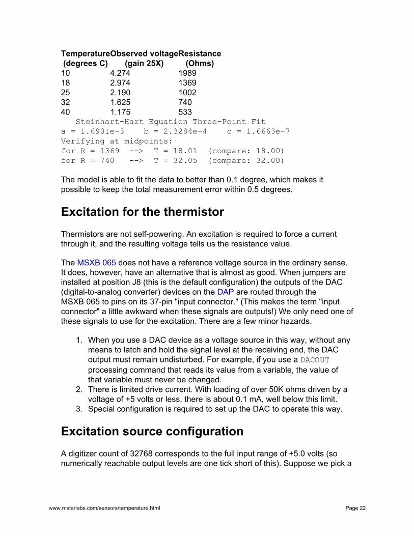
TemperatureObserved voltageResistance (degrees C) (gain 25X) (Ohms)

10 4.274 1989 18 2.974 1369 25 2.190 1002 32 1.625 740 40 1.175 533

Steinhart-Hart Equation Three-Point Fita = 1.6901e-3 b = 2.3284e-4 c = 1.6663e-7Verifying at midpoints:for R = 1369 --> T = 18.01 (compare: 18.00)for R = 740 --> T = 32.05 (compare: 32.00)

The model is able to fit the data to better than 0.1 degree, which makes it possible to keep the total measurement error within 0.5 degrees.

Excitation for the thermistor Thermistors are not self-powering. An excitation is required to force a current through it, and the resulting voltage tells us the resistance value.

The MSXB 065 does not have a reference voltage source in the ordinary sense. It does, however, have an alternative that is almost as good. When jumpers are installed at position J8 (this is the default configuration) the outputs of the DAC (digital-to-analog converter) devices on the DAP are routed through the MSXB 065 to pins on its 37-pin "input connector." (This makes the term "input connector" a little awkward when these signals are outputs!) We only need one of these signals to use for the excitation. There are a few minor hazards.

1. When you use a DAC device as a voltage source in this way, without any means to latch and hold the signal level at the receiving end, the DAC output must remain undisturbed. For example, if you use a DACOUT processing command that reads its value from a variable, the value of that variable must never be changed.

2. There is limited drive current. With loading of over 50K ohms driven by a voltage of +5 volts or less, there is about 0.1 mA, well below this limit.

3. Special configuration is required to set up the DAC to operate this way.

Excitation source configuration A digitizer count of 32768 corresponds to the full input range of +5.0 volts (so numerically reachable output levels are one tick short of this). Suppose we pick a




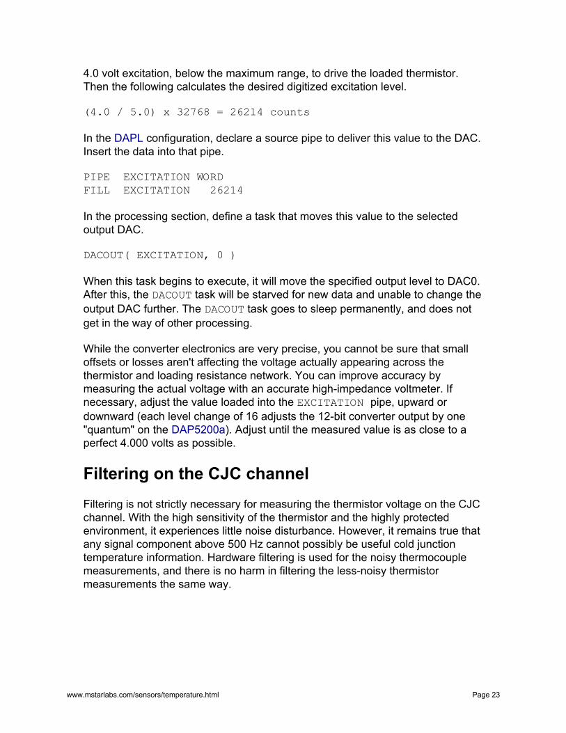
4.0 volt excitation, below the maximum range, to drive the loaded thermistor. Then the following calculates the desired digitized excitation level.

(4.0 / 5.0) x 32768 = 26214 counts

In the DAPL configuration, declare a source pipe to deliver this value to the DAC. Insert the data into that pipe.

PIPE EXCITATION WORDFILL EXCITATION 26214

In the processing section, define a task that moves this value to the selected output DAC.

DACOUT( EXCITATION, 0 )

When this task begins to execute, it will move the specified output level to DAC0. After this, the DACOUT task will be starved for new data and unable to change the output DAC further. The DACOUT task goes to sleep permanently, and does not get in the way of other processing.

While the converter electronics are very precise, you cannot be sure that small offsets or losses aren't affecting the voltage actually appearing across the thermistor and loading resistance network. You can improve accuracy by measuring the actual voltage with an accurate high-impedance voltmeter. If necessary, adjust the value loaded into the EXCITATION pipe, upward or downward (each level change of 16 adjusts the 12-bit converter output by one "quantum" on the DAP5200a). Adjust until the measured value is as close to a perfect 4.000 volts as possible.

Filtering on the CJC channel Filtering is not strictly necessary for measuring the thermistor voltage on the CJC channel. With the high sensitivity of the thermistor and the highly protected environment, it experiences little noise disturbance. However, it remains true that any signal component above 500 Hz cannot possibly be useful cold junction temperature information. Hardware filtering is used for the noisy thermocouple measurements, and there is no harm in filtering the less-noisy thermistor measurements the same way.




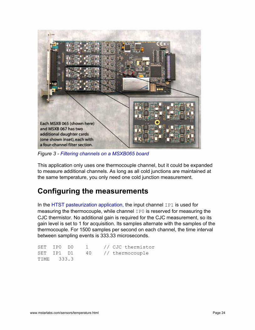
Figure 3 - Filtering channels on a MSXB065 board

This application only uses one thermocouple channel, but it could be expanded to measure additional channels. As long as all cold junctions are maintained at the same temperature, you only need one cold junction measurement.

Configuring the measurements In the HTST pasteurization application, the input channel IP1 is used for measuring the thermocouple, while channel IP0 is reserved for measuring the CJC thermistor. No additional gain is required for the CJC measurement, so its gain level is set to 1 for acquisition. Its samples alternate with the samples of the thermocouple. For 1500 samples per second on each channel, the time interval between sampling events is 333.33 microseconds.

SET IP0 D0 1 // CJC thermistorSET IP1 D1 40 // thermocoupleTIME 333.3


http://www.mstarlabs.com/access/filtermodules.html

http://www.mstarlabs.com/access/filtermodules.html

The DAP 5000a processing capacity is useful for independently processing the CJC temperature readings in parallel with the You can export the thermocouple readings. Changes in the cold configurations you develop junction temperature will be very slow, so with DAPstudio software, simple averaging that reduces each set of 10 and run them on your DAP thermistor measurements to one averaged independent of DAPstudio measurement will do the trick. Multi-tasking is or other GUI packages. automatic in the DAPL system.

// Noise and rate reduction by filteringAVERAGE(IP0, 10, PAMBIENT) // cold junctionFIRLOWPASS(IP1, 10, PREDUCED) // thermocouple

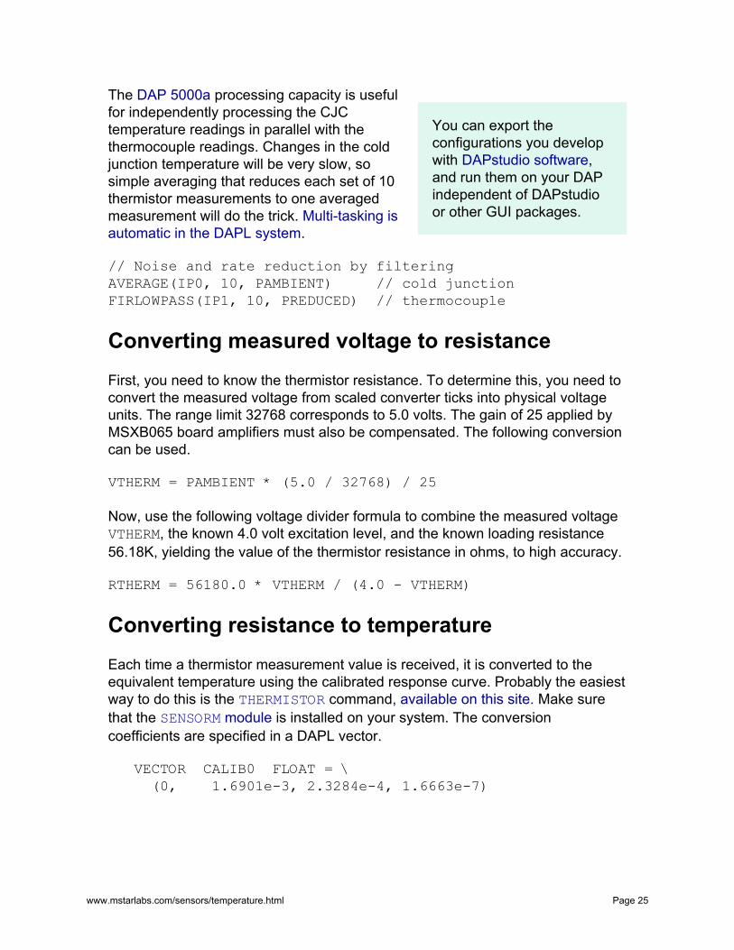
Converting measured voltage to resistance First, you need to know the thermistor resistance. To determine this, you need to convert the measured voltage from scaled converter ticks into physical voltage units. The range limit 32768 corresponds to 5.0 volts. The gain of 25 applied by MSXB065 board amplifiers must also be compensated. The following conversion can be used.

VTHERM = PAMBIENT * (5.0 / 32768) / 25

Now, use the following voltage divider formula to combine the measured voltage VTHERM, the known 4.0 volt excitation level, and the known loading resistance 56.18K, yielding the value of the thermistor resistance in ohms, to high accuracy.

RTHERM = 56180.0 * VTHERM / (4.0 - VTHERM)

Converting resistance to temperature Each time a thermistor measurement value is received, it is converted to the equivalent temperature using the calibrated response curve. Probably the easiest way to do this is the THERMISTOR command, available on this site. Make sure that the SENSORM module is installed on your system. The conversion coefficients are specified in a DAPL vector.

VECTOR CALIB0 FLOAT = \(0, 1.6901e-3, 2.3284e-4, 1.6663e-7)


http://www.mstarlabs.com/dapstudio/tabs.html


http://www.mstarlabs.com/software/dapl/multitasking.html

http://www.mstarlabs.com/software/dapl/multitasking.html



Later, in the processing section, specify this device model as you convert the measurements into temperatures. Another useful way to apply

device-specific calibrations is the DAPL system's SCALE command.

THERMISTOR(RTHERM, CALIB0, PCOLDJUNC)

To complete the processing, combine the cold junction temperature result with the temperature difference result from the thermocouple.

TADJUSTED = ... // apply thermocouple calibrationTEMPERATURE = TADJUSTED + PCOLDJUNC

Now you can route the stream of TEMPERATURE measurements to any location you wish, test the range and signal alarms in real time, collect statistics for data logging, etc.


http://www.mstarlabs.com/software/dapl/dapl-signal-conditioning.html

Calibrate Temperature SensorsWhat is sensor calibration? When using temperature sensors, you are actually measuring a voltage, and relating that to what the operating temperature of the sensor must be. If you can avoid errors in the voltage measurements, and represent the relationship between voltage and temperature more accurately, you can get better temperature readings. How much effort is worthwhile depends on the application's error tolerances.

There are four adjustments that a good calibration can provide.

• OFFSET All voltages are measured with respect to a reference. All devices operate at some operating voltage. Any displacements in these voltages, or any consistent errors during measurement, will produce consistent errors that affect all measurements. Offset corrections make these errors as small as possible.

• GAIN The voltage that you measure is not really the voltage present on the sensor device. Amplifiers and attenuation between the sensor and the digitizing converter change the signal level. To recover the sensor information, you must restore the data to the original level accurately. Uncorrected gain errors tend to produce measurement errors that change consistently across the operating range.

• LINEARIZATION The relationship between measured voltage and sensed temperature is in general nonlinear and dependent on the physical properties of each sensor type. Over a limited


TemperatureSensors


RTD Calibration


range, a simple linear function is often a sufficient approximation, but a more complicated curve is necessary to describe the relationship accurately. Generalized curves defined by standards help, but they won't match any individual device perfectly. For best accuracy, you need to calibrate, and adjust the coefficient values of the conversion function.


After applying the offset, gain, and linearization corrections, the results might not be in the most useful form. A good follow-up step is the following:

• UNIT SCALING Convert the results to a common and useful representation. For example, present all temperature measurements in degrees C.

Calibrating linearization curves

Calibration is a process of aligning what your formulas say with what real devices actually do. This involves taking some accurate measurements.

You can't control what a sensor does directly. It responds based on its physical properties. But you can to some extent control what your sensor measures. You can establish a set of temperature levels that span the operating range, and measure those levels with a laboratory-grade temperature standard. For each of those measured temperature points, observe the response level of the sensor. If you construct a curve that passes through these points, you will have a very good calibration specialized for the individual sensor.

Given the temperature vs. voltage data set, treat the sensor readings as noisy input values, and the temperature measurements as the corresponding output values to be produced. Taking multiple measurements and averaging them helps to obtain the best possible data quality for calibration.

From here, there are two ways that you can go.

1. Explicit function. Use a processing command that applies a "calibrated conversion function" for each measurement. This can be a very generic calculation like a DAPL expression or a GENPOLY command, or it can be a specialized conversion such as the RTD command.

2. Piece-wise linear approximation. Select a set of representative points along the curve and approximate the curve with straight lines "point to point." Code the "breakpoints" as vectors and supply them to the DAPL command INTERP, which can then locate the appropriate line section and evaluate the function at intermediate points.

For more information about the linearization curves most commonly used for temperature sensor calibration, check the following.

• Calibrate thermocouples • Calibrate RTDs • Calibrate thermistors


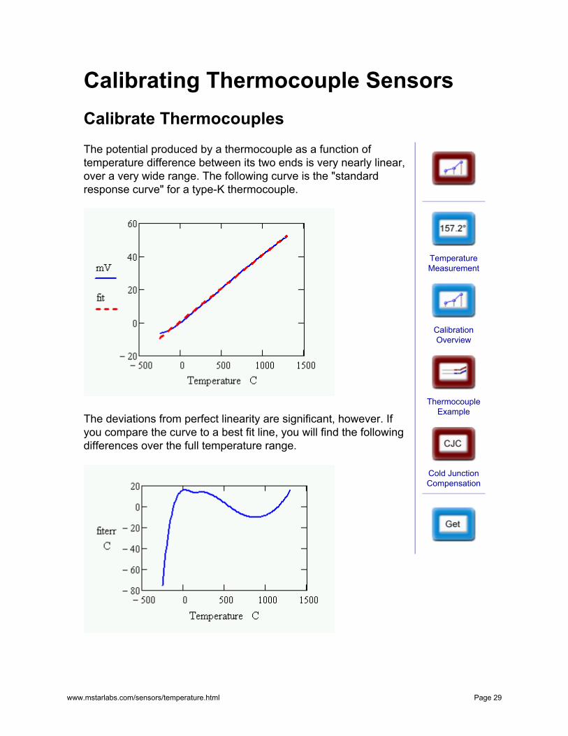
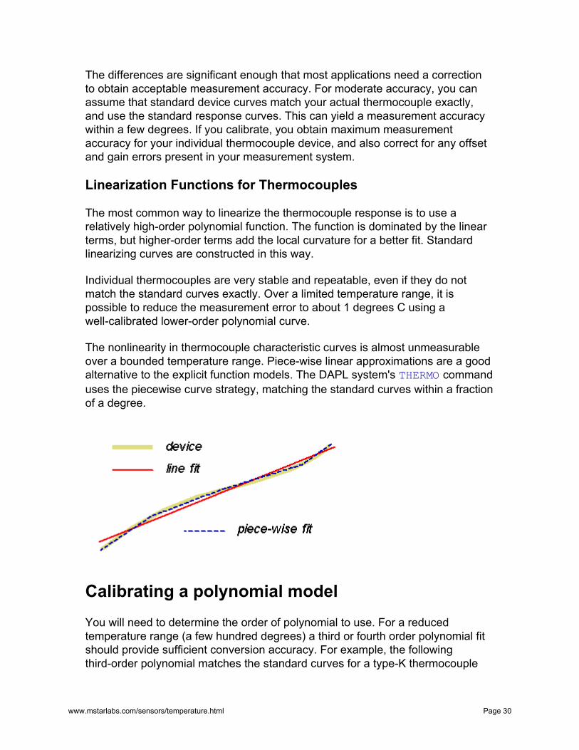
Calibrating Thermocouple SensorsCalibrate Thermocouples The potential produced by a thermocouple as a function of temperature difference between its two ends is very nearly linear, over a very wide range. The following curve is the "standard response curve" for a type-K thermocouple.

The deviations from perfect linearity are significant, however. If you compare the curve to a best fit line, you will find the following differences over the full temperature range.


CalibrationOverview

ThermocoupleExample




The differences are significant enough that most applications need a correction to obtain acceptable measurement accuracy. For moderate accuracy, you can assume that standard device curves match your actual thermocouple exactly, and use the standard response curves. This can yield a measurement accuracy within a few degrees. If you calibrate, you obtain maximum measurement accuracy for your individual thermocouple device, and also correct for any offset and gain errors present in your measurement system.

Linearization Functions for Thermocouples

The most common way to linearize the thermocouple response is to use a relatively high-order polynomial function. The function is dominated by the linear terms, but higher-order terms add the local curvature for a better fit. Standard linearizing curves are constructed in this way.

Individual thermocouples are very stable and repeatable, even if they do not match the standard curves exactly. Over a limited temperature range, it is possible to reduce the measurement error to about 1 degrees C using a well-calibrated lower-order polynomial curve.

The nonlinearity in thermocouple characteristic curves is almost unmeasurable over a bounded temperature range. Piece-wise linear approximations are a good alternative to the explicit function models. The DAPL system's THERMO command uses the piecewise curve strategy, matching the standard curves within a fraction of a degree.

Calibrating a polynomial model You will need to determine the order of polynomial to use. For a reduced temperature range (a few hundred degrees) a third or fourth order polynomial fit should provide sufficient conversion accuracy. For example, the following third-order polynomial matches the standard curves for a type-K thermocouple


http://www.mstarlabs.com/apeng/integration/thermapp.html

with error less than 0.1 degrees C through the range -45 degrees C to +150 degrees C.

T = -0.01897 + 25.41881 V - 0.42456 V2 + 0.04365 V3where V is voltage in units of millivoltsand T is temperature in degrees C

You can modify the coefficients slightly to make the conversion curve match an individual device's response for best accuracy. The calibration data must be captured very carefully, but the process is straightforward.

1. Establish stable temperatures throughout the full operating range that you intend to cover.

2. Measure each temperature carefully using an accurate measurement standard.

3. Take many measurements of the noisy thermocouple potential at each temperature point, averaging these measurements to reduce noise.

4. Collect the temperature-potential data pairs, and apply a least-squares curve fitting analysis to obtain a polynomial that best predicts the temperature given the junction potential.

Calibrating a piece-wise linear model It typically takes about 20 linear pieces to adequately approximate thermocouple standard curves. For better accuracy, more pieces should be used. Assume that the number of sections is increased to 40, then reduce the number of pieces in proportion to the fraction of the total range your application needs. So for example, a type-K thermocouple has a range of about 1600 degrees C. A temperature range of 200 degrees C is 1/8 of that, so a calibrated model with about 40/8 = 5 pieces should produce good conversion accuracy.

Knowing that the response will be nearly linear for each of the pieces, you don't need to measure everywhere as you do with a polynomial fit. For an N-piece model, measure at the two ends of the temperature range, and also at N-1 roughly evenly-spaced intermediate points. Use the same precautions as with a polynomial fit, allowing temperatures to stabilize, and taking multiple measurements at each selected point for noise reduction. You can then code the monotonically-increasing voltage terms as a vector of input x-values, and the corresponding temperature levels as a vector of y-values. Provide these two vectors to the INTERP command to evaluate your piecewise curve at any point.


Calibrating cold junction effects You can read more about the principles and application of cold junction compensation in another page on this site.

There are some practical limitations on the accuracy you can achieve when using the LT1025A temperature measurement devices available on MSTB009 termination boards, and optionally available on MSXB037 analog expansion boards.

1. The baseline temperature measurement error of the chip is 0.5 degrees C.

2. Even when you bring the thermocouple wires all the way to termination board terminals, physically close to the location of the temperature measurement chip, it is difficult to maintain perfectly uniform temperatures across the termination board. You are doing very well if you can hold this error to an additional 0.5 degrees C.

3. Calibrating the sensor chips would require controlling the board environment to a number of stable and accurately measured operating temperatures. This is probably infeasible.

The bottom line: any errors in reading the cold junction temperature will contribute directly to errors in the final temperature measurement. Expect at least 1 degree error from cold junction measurements when using the on-board temperature memeasurement circuits.

For better accuracy, you will need better control and calibration of your cold junction measurements. An application using a separate calibrated temperature sensor for best cold junction measurement accuracy is described in an application note on this site.

Thermocouple applications that do not calibrate cannot do much better than the THERMO command provided by the DAPL system. For evaluating customized piecewise-linear curves, you can use the INTERP command, also provided by the DAPL system. For evaluating polynomial models, you can use the generic polynomial evaluator command GENPOLY available on this site. Or for a special case that also covers cold junction compensation, you can use the THERMOPOLY command available on this site.


http://www.mstarlabs.com/access/tb009.html








Cold junction compensation Thermocouple Cold Junctions The terms hot junction and cold junction, as applied to thermocouple devices, are mostly historical. You don't need to have any junctions to get thermocouple effects. If you heat one end of a metal conductor and hold the other end at a constant reference temperature, two important things occur.

1. Heat flow. There is a thermal gradient, so heat flows from the hot end to the cold end. With small-gage thermocouple wire, very little thermal energy actually reaches the cold end, and the thermal gradient is typically not constant along the wires because of heat loss.

2. Seebeck effect. Energetic electrons at the hot end diffuse toward the cold end, pushing less energetic electrons along with them, resulting in a higher static potential at the hot end relative to the cold end. The larger the temperature gradient, the larger the potential difference. (There are additional contributing effects when dissimilar materials are joined.)

In practice, it is difficult to measure the Seebeck effect directly. When you attach measurement probes, there is a thermal difference across the probe leads, producing additional thermocouple effects that interfere with the measurements.

Classical thermocouple loop configuration

To make the thermal effects measurable, two different metal conductors are used. They must be chemically, electrically, and physically compatible. They produce different electric potentials when subjected to the same thermal gradient.


CalibrationOverview

ThermocoupleExample


In the classical configuration, the dissimilar thermocouple wires are welded together at the measurement end (hot junction), and again at the reference end (cold junction), forming a loop. The hot junction assures that the potential at that point matches in the two metals. Immersing the reference-end junction in an ice-water slurry assures that the temperature gradients are the same across both materials. The ice-water slurry establishes a reference temperature at 0 degrees C.



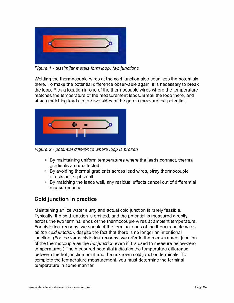
Figure 1 - dissimilar metals form loop, two junctions

Welding the thermocouple wires at the cold junction also equalizes the potentials there. To make the potential difference observable again, it is necessary to break the loop. Pick a location in one of the thermocouple wires where the temperature matches the temperature of the measurement leads. Break the loop there, and attach matching leads to the two sides of the gap to measure the potential.

Figure 2 - potential difference where loop is broken

• By maintaining uniform temperatures where the leads connect, thermal gradients are unaffected.

• By avoiding thermal gradients across lead wires, stray thermocouple effects are kept small.

• By matching the leads well, any residual effects cancel out of differential measurements.

Cold junction in practice

Maintaining an ice water slurry and actual cold junction is rarely feasible. Typically, the cold junction is omitted, and the potential is measured directly across the two terminal ends of the thermocouple wires at ambient temperature. For historical reasons, we speak of the terminal ends of the thermocouple wires as the cold junction, despite the fact that there is no longer an intentional junction. (For the same historical reasons, we refer to the measurement junction of the thermocouple as the hot junction even if it is used to measure below-zero temperatures.) The measured potential indicates the temperature difference between the hot junction point and the unknown cold junction terminals. To complete the temperature measurement, you must determine the terminal temperature in some manner.


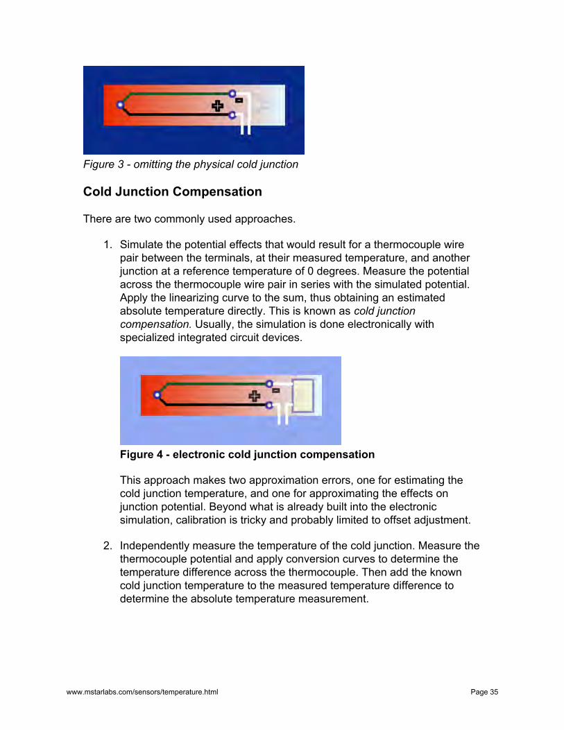
Figure 3 - omitting the physical cold junction

Cold Junction Compensation

There are two commonly used approaches.

1. Simulate the potential effects that would result for a thermocouple wire pair between the terminals, at their measured temperature, and another junction at a reference temperature of 0 degrees. Measure the potential across the thermocouple wire pair in series with the simulated potential. Apply the linearizing curve to the sum, thus obtaining an estimated absolute temperature directly. This is known as cold junction compensation. Usually, the simulation is done electronically with specialized integrated circuit devices.

Figure 4 - electronic cold junction compensation

This approach makes two approximation errors, one for estimating the cold junction temperature, and one for approximating the effects on junction potential. Beyond what is already built into the electronic simulation, calibration is tricky and probably limited to offset adjustment.

2. Independently measure the temperature of the cold junction. Measure the thermocouple potential and apply conversion curves to determine the temperature difference across the thermocouple. Then add the known cold junction temperature to the measured temperature difference to determine the absolute temperature measurement.


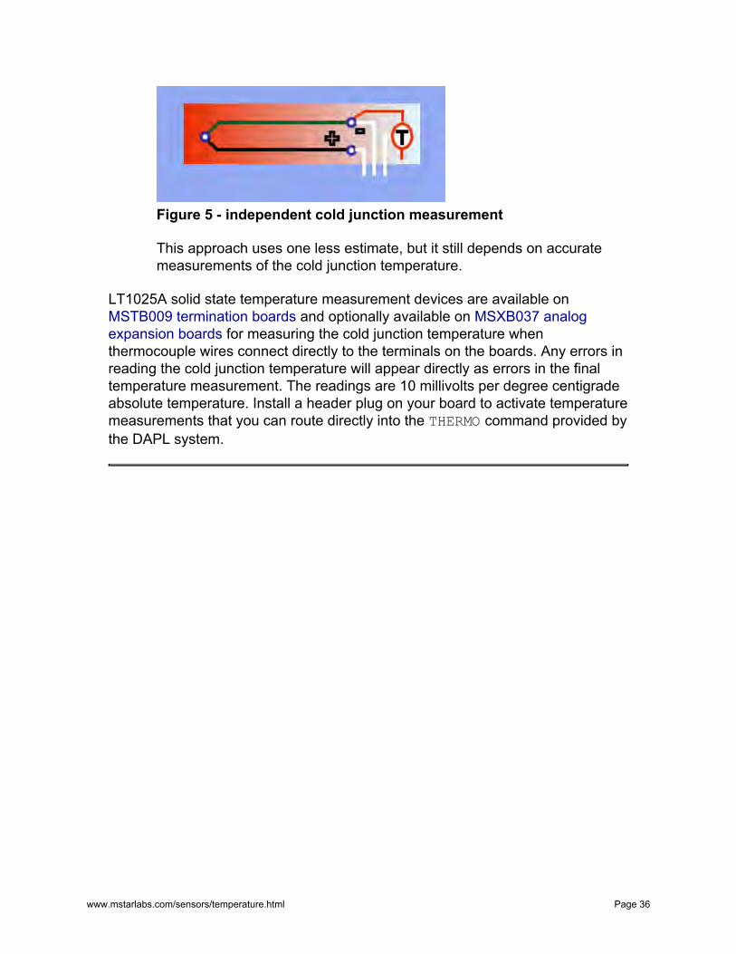
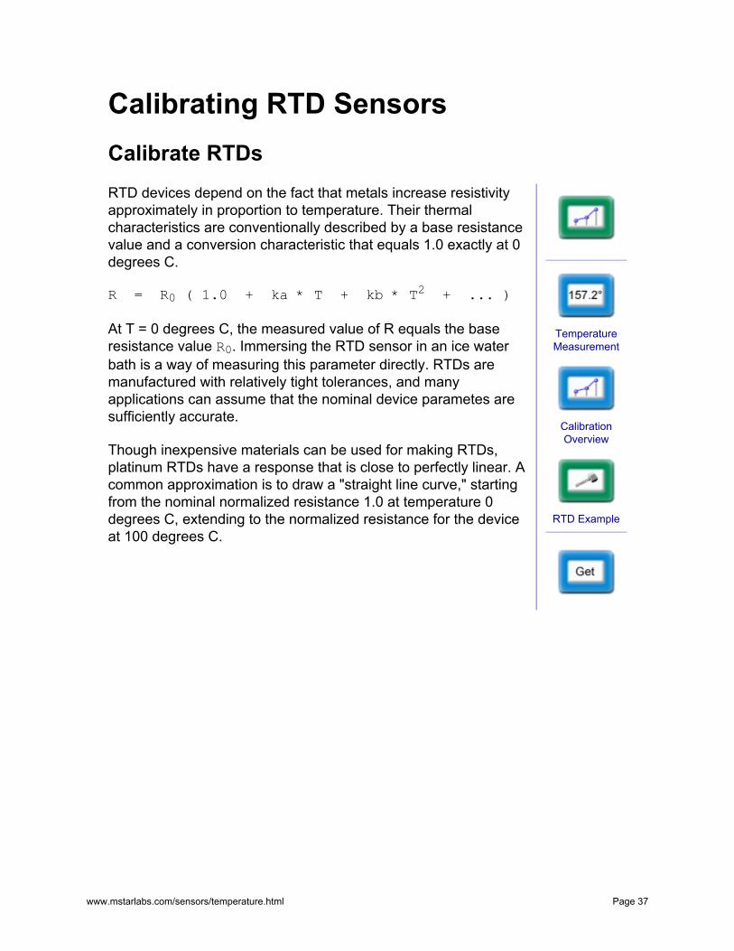
Figure 5 - independent cold junction measurement

This approach uses one less estimate, but it still depends on accurate measurements of the cold junction temperature.

LT1025A solid state temperature measurement devices are available on MSTB009 termination boards and optionally available on MSXB037 analog expansion boards for measuring the cold junction temperature when thermocouple wires connect directly to the terminals on the boards. Any errors in reading the cold junction temperature will appear directly as errors in the final temperature measurement. The readings are 10 millivolts per degree centigrade absolute temperature. Install a header plug on your board to activate temperature measurements that you can route directly into the THERMO command provided by the DAPL system.





Calibrating RTD Sensors Calibrate RTDs RTD devices depend on the fact that metals increase resistivity approximately in proportion to temperature. Their thermal characteristics are conventionally described by a base resistance value and a conversion characteristic that equals 1.0 exactly at 0 degrees C.

R = R0 ( 1.0 + ka * T + kb * T2 + ... )

At T = 0 degrees C, the measured value of R equals the base resistance value R0. Immersing the RTD sensor in an ice water bath is a way of measuring this parameter directly. RTDs are manufactured with relatively tight tolerances, and many applications can assume that the nominal device parametes are sufficiently accurate.

Though inexpensive materials can be used for making RTDs, platinum RTDs have a response that is close to perfectly linear. A common approximation is to draw a "straight line curve," starting from the nominal normalized resistance 1.0 at temperature 0 degrees C, extending to the normalized resistance for the device at 100 degrees C.


CalibrationOverview

RTD Example



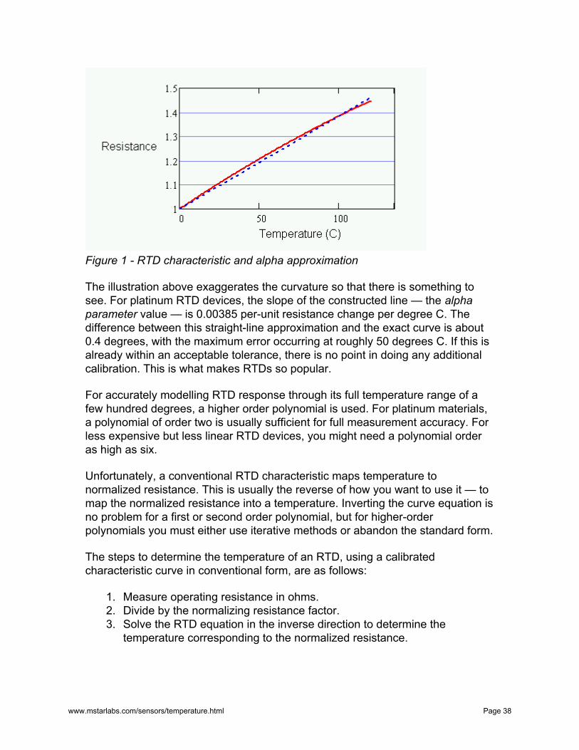
Figure 1 - RTD characteristic and alpha approximation

The illustration above exaggerates the curvature so that there is something to see. For platinum RTD devices, the slope of the constructed line — the alpha parameter value — is 0.00385 per-unit resistance change per degree C. The difference between this straight-line approximation and the exact curve is about 0.4 degrees, with the maximum error occurring at roughly 50 degrees C. If this is already within an acceptable tolerance, there is no point in doing any additional calibration. This is what makes RTDs so popular.

For accurately modelling RTD response through its full temperature range of a few hundred degrees, a higher order polynomial is used. For platinum materials, a polynomial of order two is usually sufficient for full measurement accuracy. For less expensive but less linear RTD devices, you might need a polynomial order as high as six.

Unfortunately, a conventional RTD characteristic maps temperature to normalized resistance. This is usually the reverse of how you want to use it — to map the normalized resistance into a temperature. Inverting the curve equation is no problem for a first or second order polynomial, but for higher-order polynomials you must either use iterative methods or abandon the standard form.

The steps to determine the temperature of an RTD, using a calibrated characteristic curve in conventional form, are as follows:

1. Measure operating resistance in ohms. 2. Divide by the normalizing resistance factor. 3. Solve the RTD equation in the inverse direction to determine the

temperature corresponding to the normalized resistance.


Usually it is most efficient to compute RTD characteristic curves directly. As with any sensor, it is possible to select corner points at intervals along the characteristic curve and represent the inverse curve with a piece-wise linear approximation, and evaluate it using the INTERP command. Intervals of about 50 degrees C should work well.

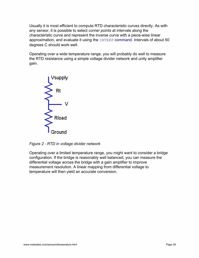
Operating over a wide temperature range, you will probably do well to measure the RTD resistance using a simple voltage divider network and unity amplifier gain.

Figure 2 - RTD in voltage divider network

Operating over a limited temperature range, you might want to consider a bridge configuration. If the bridge is reasonably well balanced, you can measure the differential voltage across the bridge with a gain amplifier to improve measurement resolution. A linear mapping from differential voltage to temperature will then yield an accurate conversion.


http://www.mstarlabs.com/software/dapl/dapl-signal-conditioning.html

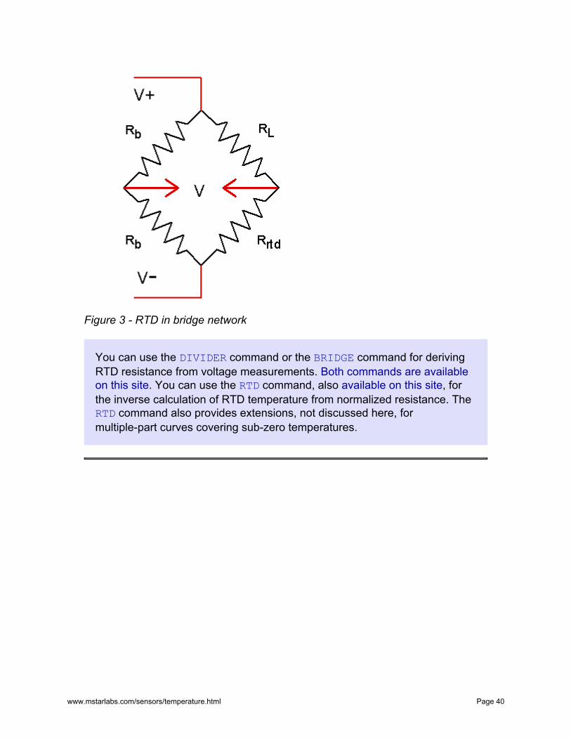
Figure 3 - RTD in bridge network

You can use the DIVIDER command or the BRIDGE command for deriving RTD resistance from voltage measurements. Both commands are available on this site. You can use the RTD command, also available on this site, for the inverse calculation of RTD temperature from normalized resistance. The RTD command also provides extensions, not discussed here, for multiple-part curves covering sub-zero temperatures.





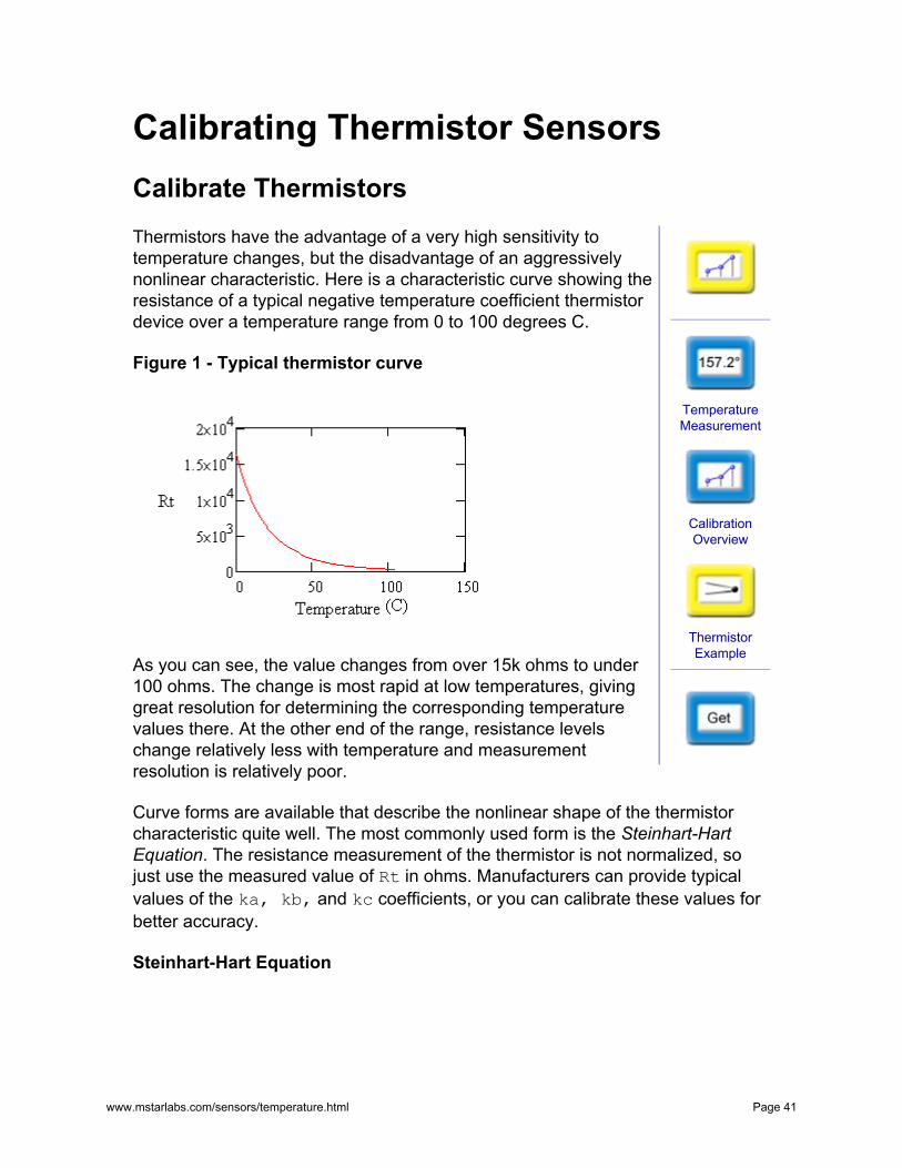
Calibrating Thermistor SensorsCalibrate Thermistors Thermistors have the advantage of a very high sensitivity to temperature changes, but the disadvantage of an aggressively nonlinear characteristic. Here is a characteristic curve showing the resistance of a typical negative temperature coefficient thermistor device over a temperature range from 0 to 100 degrees C.

Figure 1 - Typical thermistor curve

Temperature Measurement

Calibration Overview

Thermistor Example

As you can see, the value changes from over 15k ohms to under 100 ohms. The change is most rapid at low temperatures, giving great resolution for determining the corresponding temperature values there. At the other end of the range, resistance levels change relatively less with temperature and measurement resolution is relatively poor.

Curve forms are available that describe the nonlinear shape of the thermistor characteristic quite well. The most commonly used form is the Steinhart-Hart Equation. The resistance measurement of the thermistor is not normalized, so just use the measured value of Rt in ohms. Manufacturers can provide typical values of the ka, kb, and kc coefficients, or you can calibrate these values for better accuracy.

Steinhart-Hart Equation



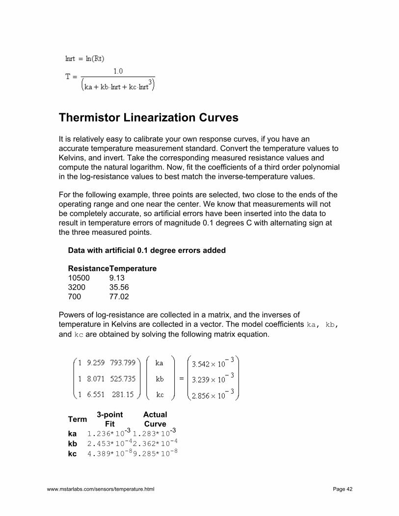
Thermistor Linearization Curves It is relatively easy to calibrate your own response curves, if you have an accurate temperature measurement standard. Convert the temperature values to Kelvins, and invert. Take the corresponding measured resistance values and compute the natural logarithm. Now, fit the coefficients of a third order polynomial in the log-resistance values to best match the inverse-temperature values.

For the following example, three points are selected, two close to the ends of the operating range and one near the center. We know that measurements will not be completely accurate, so artificial errors have been inserted into the data to result in temperature errors of magnitude 0.1 degrees C with alternating sign at the three measured points.

Data with artificial 0.1 degree errors added

ResistanceTemperature 10500 9.13 3200 35.56 700 77.02

Powers of log-resistance are collected in a matrix, and the inverses of temperature in Kelvins are collected in a vector. The model coefficients ka, kb, and kc are obtained by solving the following matrix equation.

Term 3-point Actual Fit Curve

ka 1.236*10-3 1.283*10-3

kb 2.453*10-42.362*10-4 kc 4.389*10-89.285*10-8


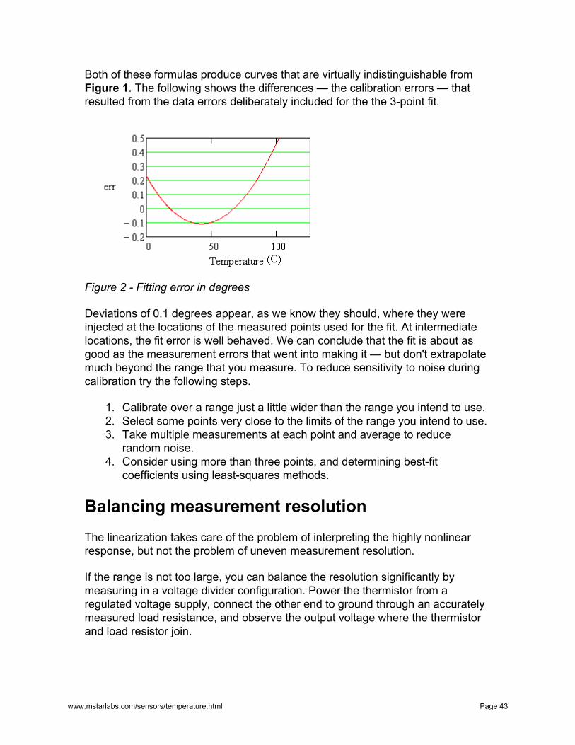
Both of these formulas produce curves that are virtually indistinguishable from Figure 1. The following shows the differences — the calibration errors — that resulted from the data errors deliberately included for the the 3-point fit.

Figure 2 - Fitting error in degrees

Deviations of 0.1 degrees appear, as we know they should, where they were injected at the locations of the measured points used for the fit. At intermediate locations, the fit error is well behaved. We can conclude that the fit is about as good as the measurement errors that went into making it — but don't extrapolate much beyond the range that you measure. To reduce sensitivity to noise during calibration try the following steps.

1. Calibrate over a range just a little wider than the range you intend to use. 2. Select some points very close to the limits of the range you intend to use. 3. Take multiple measurements at each point and average to reduce

random noise. 4. Consider using more than three points, and determining best-fit

coefficients using least-squares methods.

Balancing measurement resolution The linearization takes care of the problem of interpreting the highly nonlinear response, but not the problem of uneven measurement resolution.

If the range is not too large, you can balance the resolution significantly by measuring in a voltage divider configuration. Power the thermistor from a regulated voltage supply, connect the other end to ground through an accurately measured load resistance, and observe the output voltage where the thermistor and load resistor join.


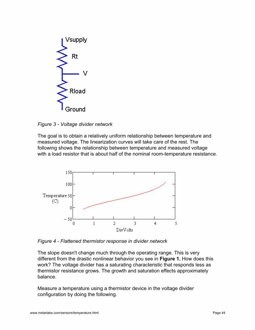
Figure 3 - Voltage divider network

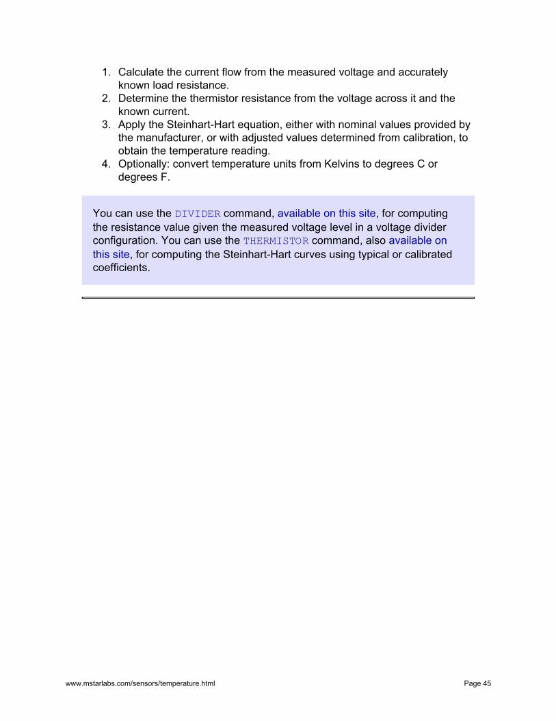
The goal is to obtain a relatively uniform relationship between temperature and measured voltage. The linearization curves will take care of the rest. The following shows the relationship between temperature and measured voltage with a load resistor that is about half of the nominal room-temperature resistance.

Figure 4 - Flattened thermistor response in divider network

The slope doesn't change much through the operating range. This is very different from the drastic nonlinear behavior you see in Figure 1. How does this work? The voltage divider has a saturating characteristic that responds less as thermistor resistance grows. The growth and saturation effects approximately balance.

Measure a temperature using a thermistor device in the voltage divider configuration by doing the following.


1. Calculate the current flow from the measured voltage and accuratelyknown load resistance.

2. Determine the thermistor resistance from the voltage across it and the known current.

3. Apply the Steinhart-Hart equation, either with nominal values provided by the manufacturer, or with adjusted values determined from calibration, to obtain the temperature reading.

4. Optionally: convert temperature units from Kelvins to degrees C ordegrees F.

You can use the DIVIDER command, available on this site, for computing the resistance value given the measured voltage level in a voltage divider configuration. You can use the THERMISTOR command, also available on this site, for computing the Steinhart-Hart curves using typical or calibrated coefficients.





Module SENSORM :: BRIDGEDAPL Operating System | Processing Commands

Convert measurements from a balanced bridge network to determine resistance.

Syntax

BRIDGE( VIN, VS, BALANCE, RLOAD,[RCOEFF, LTMP,] [GAIN,] ROUT )

Parameters

VINInput data pipe with bridge imbalance voltage measurements

FLOAT PIPE

VSNominal or measured excitation voltage driving bridge network

FLOAT CONSTANT | FLOAT PIPE

BALANCENominal or measured balancing network gain

FLOAT CONSTANT

RLOADNominal or calibrated load resistance, ohms at 0 degrees C

FLOAT CONSTANT

RCOEFFTemperature coefficient of resistance of load resistor, ohms per degree C

FLOAT CONSTANT

LTMPInput pipe with load temperature measurements, degrees C


FLOAT PIPE

GAINThe gain used to measure the VIN signal

FLOAT CONSTANT

ROUTOutput resistance measurements, in ohms

FLOAT PIPE

Description

The BRIDGE command converts the differential voltage readings from VIN tomeasure an unknown resistance in a bridge network configuration. Current froma known voltage supply drives a load resistance, and then passes through theunknown device to the drain voltage. On the other side of the bridge network, twoknown resistors form a voltage divider to establish a reference voltage. Thedifferential measurements of voltage between the measurement and referencesides of the bridge are used to calculate the values of the unknown resistance,with results placed into the ROUT pipe, one output value for each input value.

The differential input measurement will reject "common mode" voltages, so itdoes not matter whether the bridge circuit is excited by balanced plus/minussupplies or a single-sided supply, as long as the common mode voltage is withina measurable range. Bridge configurations are useful when the measuredchanges in resistance are relatively small and ride on top of a relatively largeconstant level. The differential voltage can be measured with gain to improveresolution. If a gain other than 1.0 is used, either specify it as the value of theGAIN parameter, or correct for the gain prior to sending the VIN data to theBRIDGE command.

If the supply voltage is very well regulated, it can be specified as a constant VSparameter. For best accuracy, measure the actual supply voltage accuratelyrather than assuming a nominal value. If the supply is subject to small butrelevant variations, measure its voltage simultaneously and pass thesemeasurements in units of volts through a VS pipe, with one supply voltagemeasurement per divider voltage reading. If you have balanced plus and minussupplies, specify the supply-to-supply voltage.

Ideally, the voltage dividers on the reference and measurement sides of thebridge produce exactly the same voltage at a suitable reference operating pointwithin the normal operating range. Obtaining a perfect balance is hard to achieve


and not really necessary. Measure the resistances in the balancing networkaccurately, then set the BALANCE parameter equal to the ratio

BALANCE = Rg / (Rs + Rg)

where Rs is the balancing resistor on the positive supply sideand Rg is the balancing resistor on the negative supply or

ground side

If measurement accuracy is not critical, use nominal values of the resistors todetermine the value of the BALANCE parameter. Good balancing resistors willnot cause excessive power supply loading, and will establish a zero differentialreading near the center of the operating range.

Resistors in the balancing network are presumed to be located in a controlledoperating environment where small temperature variations affect both balancingresistors the same, hence the ratio remains very stable. If the loading resistor isalso located in a controlled environment, it too can be presumed to maintain aconsistent operating temperature. Specify an accurately measured value of theRLOAD parameter at the stable operating temperature, in ohms. If accuracy isnot critical, use the nominal loading resistor value.

When load temperature is not so well controlled and there is significant thermalvariation in the loading resistor, use the optional RCOEFF and LTMP parameters.Set the RCOEFF parameter to the temperature coefficient of load resistance inohms per degree Centigrade. Adjust the RLOAD parameter if necessary so that itequals the correct loading resistance at 0 degrees Centigrade. Independentlymeasure the load temperature in units of degrees Centigrade, and send thesereadings to the BRIDGE command through the LTMP pipe. The BRIDGEcommand will adjust the value of the loading resistor prior to each conversion.

For each input voltage measurement, the reference voltage on the balancing sideof the bridge is equal to the BALANCE ratio times the excitation voltage. Thevoltage on the active side of the bridge equals this reference voltage plus themeasured differential voltage. The voltage between the positive source and themeasurement point appears across the known loading resistance, so themeasurement-side current can be computed. Using the value of this current, andthe known voltage on the measurement side of the bridge, the unknown value ofresistance can be calculated.

Examples

BRIDGE(IP2, 5.0, 0.5, 1000.0, R2)


Voltage measurements are taken for a bridge configuration in which nominalvalues of components are used. The voltage at the active divider junction,relative to the balancing network junction, is obtained from the differential inputsample channel pipe IPipe 2. The excitation voltage is a nominal 5.0 volts.The nominal balancing ratio with equal-value balancing resistors is 0.5. Theloading resistor is 1K, equal to the nominal operating value of the measuredresistance. Default measurement gain of 1.0 is assumed. The computedresistance values are reported in pipe R2.

BRIDGE(IP2, 4.959, 0.5025, 1001.8, 0.087, TLOAD, 10.0, R2)

The same as the previous configuration, except that all components arecalibrated and the loading resistor value is compensated for temperaturevariations to obtain maximum measurement accuracy. The supply voltage ismeasured at 4.959 volts. The balancing resistors are not perfectly matched andtheir gain ratio is 0.5025. The nominal 1K loading resistance is measured at 0degrees Centigrade where it has the value 1001.8 ohms. The loading resistorvalue is observed to increase by 8.7 ohms over a 100 degree temperature swing,so the temperature coefficient is 0.087 ohms per degrees C. Independentmeasurements of the operating temperature of the load resistance are providedby pipe TLOAD. The measurements use an amplifier gain of 10.0. The results ofthe resistance calculations are returned in pipe R2.

See also:

DIVIDER


Module SENSORM :: DIVIDERDAPL Operating System | Processing Commands

Convert measurements from a voltage divider network to determine resistance.

Syntax

DIVIDER( VIN, VS, RLOAD, [RCOEFF, LTMP,] [GAIN,] ROUT )

Parameters

VINInput measurements of divider voltage

FLOAT PIPE

VSNominal or measured excitation voltage driving divider network

FLOAT CONSTANT | FLOAT PIPE

RLOADNominal or calibrated load resistance, ohms at 0 degrees C

FLOAT CONSTANT

RCOEFFTemperature coefficient of resistance for load resistor

FLOAT CONSTANT

LTMPInput pipe with load temperature measurements, degrees C

FLOAT PIPE

GAINGain used to measure input signal VIN

FLOAT CONSTANT


ROUTOutput resistance measurements, in ohms

FLOAT PIPE

Description

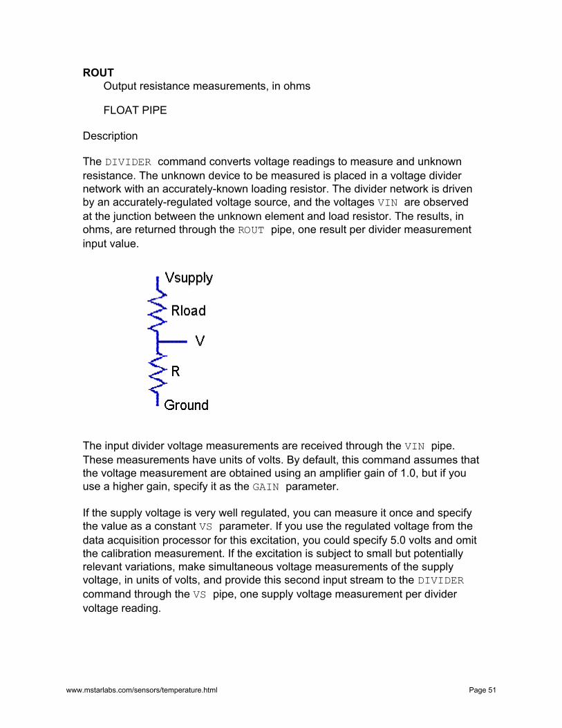
The DIVIDER command converts voltage readings to measure and unknownresistance. The unknown device to be measured is placed in a voltage dividernetwork with an accurately-known loading resistor. The divider network is drivenby an accurately-regulated voltage source, and the voltages VIN are observedat the junction between the unknown element and load resistor. The results, inohms, are returned through the ROUT pipe, one result per divider measurementinput value.

The input divider voltage measurements are received through the VIN pipe.These measurements have units of volts. By default, this command assumes thatthe voltage measurement are obtained using an amplifier gain of 1.0, but if youuse a higher gain, specify it as the GAIN parameter.

If the supply voltage is very well regulated, you can measure it once and specifythe value as a constant VS parameter. If you use the regulated voltage from thedata acquisition processor for this excitation, you could specify 5.0 volts and omitthe calibration measurement. If the excitation is subject to small but potentiallyrelevant variations, make simultaneous voltage measurements of the supplyvoltage, in units of volts, and provide this second input stream to the DIVIDERcommand through the VS pipe, one supply voltage measurement per dividervoltage reading.


Specify the loading resistor value RLOAD parameter in units of ohms. Sometimesa nominal resistor value is close enough, but for better results enter anaccurately- measured value.

Most of the time, variations in operating temperature are insignificant, and theload resistance can be presumed constant. For these cases, omit the RCOEFFand LTMP parameters. However, if significant temperature variations areanticipated, the DIVIDER command can adjust the effective load resistance tocompensate for temperature-dependent changes. Set the RCOEFF parameter tothe temperature coefficient of load resistance in ohms per degree Centigrade.Adjust the RLOAD parameter if necessary so that it reports the correct loadingresistance at 0 degrees Centigrade. Measure the load resistance temperature inunits of degrees Centigrade and send these measurements to the DIVIDERcommand through the LTMP pipe, one temperature reading per dividermeasurement.

For processing each input value, the difference between the known excitationvoltage source and the measured divider junction appears across the knownloading resistor, hence the divider current can be computed. This known dividercurrent passes through the unknown element to produce the measured voltage,so its resistance can be computed, producing the results placed into the ROUTpipe.

Examples

DIVIDER(IP2, 5.000, 10000.0, ROUT)

Read the voltage at the junction between a load resistance of exactly 10K ohmsand an unknown resistive sensor when a 5.000 volt excitation voltage is appliedacross the divider network. The voltages across the resistive sensor element aremeasured with gain 1 and received from input sample channel pipe IPipe 2.The computed resistance values are reported in pipe ROUT.

DIVIDER(IP2, 4.968, 10008.0, 0.42, PAmb, 4.0, ROUT)

This example is the same as the previous configuration, except calibrated formaximum measurement accuracy. The pre-measured supply voltage level is4.958 ohms is specified as a constant. The measured load resistor value is10008 ohms. The nominal load resistance is observed to increase by 42 ohmsover a 100 degree temperature swing, so a temperature coefficient 0.42 ohmsper degrees C is specified. The measurements of divider voltage are capturedusing an amplifier gain of 4.0. The operating temperature is separately measuredand provided in the PAmb pipe. The computations use a temperature-adjustedvalue of load resistance for each conversion.


See also:

BRIDGE


Module SENSORM :: GENPOLYDAPL Operating System | Processing Commands

Generic polynomial conversion function.

Syntax

GENPOLY( VIN, [NORDER,] VCOEFFS, VOUT )

Parameters

VINInput data values

FLOAT PIPE

NORDEROrder of the polynomial function

WORD CONSTANT

VCOEFFSCoefficients of the polynomial

FLOAT VECTOR

VOUTOutput data values

FLOAT PIPE

Description

The GENPOLY command is a general purpose mapping from a stream of inputdata received from pipe VIN, to produce a stream of output data in pipe VOUT.One common application of this command is mapping measurements of anarbitrary nonlinear sensor into the equivalent measurement in the desiredphysical units.


The polynomial mapping is determined by the VCOEFFS vector. The coefficientsspecified in this vector start with the zero-order term, followed by the first-orderterm, followed by the second-order term, etc. up to the order specified by theNORDER parameter. If you omit the NORDER parameter, the command will countterms and assume the corresponding maximum order.

Using only a first-order polynomial, this command becomes equivalent to aSCALE command. From the opposite point of view, this command covers thefunctionality of the SCALE command at the same time that it performs nonlinearmappings. When using this command for "linearizing" the response of anonlinear sensor, it can at the same time provide gain and offset corrections.

Examples

VECTOR VCOEFFS FLOAT = ( 1.0, 3.085e-3, -5.707e-7 )CONSTANT ORDER WORD = 2...GENPOLY( PIN, ORDER, VCOEFFS, POUT )

Take values X from the PIN pipe one at a time, and for each one apply thesecond-order polynomial mapping

Y = 1.0 + 3.085e-3*X + -5.707e-7*X2

to obtain the values Y that are placed into the output data stream POUT.

See also:

SCALE, RTD, THERMOPOLY


Module SENSORM :: RTDDAPL Operating System | Processing Commands

Convert resistance measurements to the corresponding temperature for an RTDdevice.

Syntax

RTD( RIN, VMODEL, TEMPOUT )

Parameters

RINInput resistance values in ohms

FLOAT PIPE

VMODELCoefficients for polynomial conversion model

FLOAT VECTOR

TEMPOUTOutput data pipe, temperatures in degrees Centigrade

FLOAT PIPE

Description

The RTD command converts resistance values received from the RIN pipe,using the device model specified by the VMODEL vector, and delivering thecorresponding output temperatures in degrees C to the TEMPOUT pipe.

Though their temperature response is almost linear, RTD devices need anonlinear conversion for full accuracy. The device model is a polynomial curve,with the number of terms required dependent on the material type used tofabricate the RTD. Devices have standardized conversion curves, but actualdevices don't always match the standardized curves perfectly. For best accuracy,


you can fit a polynomial curve to measured resistance and the correspondingtemperatures, thus calibrating your own response curves.

The following conversion characteristic for an RTD device is suitable for widetemperature ranges and a variety of RTD device types.

R = R0 ( 1.0 + c1 T + c2 T2 + c3 T3 ...)

The RTD command supports terms up to order 6. The R0 term corresponds tothe nominal resistance of the device at 0 degrees C. For example, a type JPT200RTD will have a nominal resistance of 200 ohms, and a perfectly manufactureddevice will have a base resistance R0 exactly equal to 200. The zero-order termof the conversion polynomial is always normalized to 1.0, so it is not stored, andthe base resistance value is recorded in that location.

Some curve forms provided by manufacturers and standards bodies will notcorrespond to the general polynomial form. For these, you will need to adjust thecoefficients. An important example is the platinum PT device series. It uses aconversion polynomial of the Callendar - Van Dusen form

R = R0 ( 1.0 + a1 T + a2 T2 + a3(T-100) T3 )

The appropriate conversions to the general polynomial form are:

c1 = a1c2 = a2c3 = -100.0 a3c4 = a3

There is an additional complication with standard platinum RTD devices. TheIEC751 standard specifies a different polynomial for temperatures below 0degrees C and above 0 degrees C. To allow for this, and also to allow you tocalibrate your own piecewise polynomial curves, the RTD command allowsmultiple polynomial curve sections. The nominal RTD resistance is the same forall sections. In the second, third, subsequent pieces, the zero order term locationis used to store the temperature level above which the evaluation schemeswitches to that piece of the composite curve. The additional 6 coefficient termsfor that piece follow the temperature break-point level term.

The following table provides coefficients that you can use for typical device types.


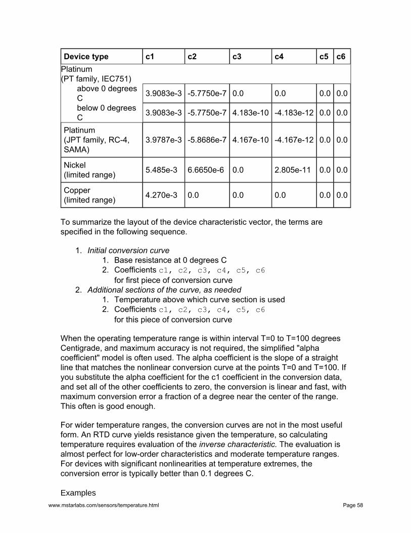
Device type c1 c2 c3 c4 c5 c6Platinum(PT family, IEC751)

above 0 degreesC 3.9083e-3 -5.7750e-7 0.0 0.0 0.0 0.0

below 0 degreesC 3.9083e-3 -5.7750e-7 4.183e-10 -4.183e-12 0.0 0.0

Platinum(JPT family, RC-4,SAMA)

3.9787e-3 -5.8686e-7 4.167e-10 -4.167e-12 0.0 0.0

Nickel(limited range) 5.485e-3 6.6650e-6 0.0 2.805e-11 0.0 0.0

Copper(limited range) 4.270e-3 0.0 0.0 0.0 0.0 0.0

To summarize the layout of the device characteristic vector, the terms arespecified in the following sequence.

1. Initial conversion curve1. Base resistance at 0 degrees C2. Coefficients c1, c2, c3, c4, c5, c6

for first piece of conversion curve2. Additional sections of the curve, as needed

1. Temperature above which curve section is used2. Coefficients c1, c2, c3, c4, c5, c6

for this piece of conversion curve

When the operating temperature range is within interval T=0 to T=100 degreesCentigrade, and maximum accuracy is not required, the simplified "alphacoefficient" model is often used. The alpha coefficient is the slope of a straightline that matches the nonlinear conversion curve at the points T=0 and T=100. Ifyou substitute the alpha coefficient for the c1 coefficient in the conversion data,and set all of the other coefficients to zero, the conversion is linear and fast, withmaximum conversion error a fraction of a degree near the center of the range.This often is good enough.

For wider temperature ranges, the conversion curves are not in the most usefulform. An RTD curve yields resistance given the temperature, so calculatingtemperature requires evaluation of the inverse characteristic. The evaluation isalmost perfect for low-order characteristics and moderate temperature ranges.For devices with significant nonlinearities at temperature extremes, theconversion error is typically better than 0.1 degrees C. Examples


VECTOR vPT100POS FLOAT = ( 100.0,3.9083e-3, -5.7750e-7, 0.0, 0.0,0.0, 0.0 )

...RTD(PRESIST,vPT100POS,TEMPR)

A type PT100 RTD is used, but temperatures never go below 0 degrees C. Thecharacteristic terms for the sub-zero piece of the standard conversion curve areomitted. Otherwise, the conversion curve in vector vPT100POS matches theIEC751 standard for this device type. The nominal 100 ohms base resistance at0 degrees C is used. When the RTD command executes, measurements ofresistance in ohms are obtained from pipe PRESIST. Each resistance value isconverted to the corresponding operating temperature of the RTD device bysolving the inverse of the device characteristic. The resulting temperatures indegrees C are placed into pipe TEMPR.

VECTOR vPT100 FLOAT = ( 99.86,3.9083e-3, -5.7750e-7, 4.1830e-10, -4.1830e-12,0.0, 0.0,

0.000,3.9083e-3, -5.7750e-7, 0.0, 0.0,0.0, 0.0 )

...RTD(PRESIST,vPT100,TEMPR)

The same example, except that temperatures can range both below and above 0degrees C. The resistance of the RTD device is calibrated by measuringaccurately at 0 degrees C, and the observed value 99.86 ohms is specified asthe base resistance. The first set of polynomial terms conform to the the IEC751standard for temperatures below 0.000 degrees. For temperatures above 0.000degrees, the conversion processing switches over to the second set of terms.

See also:

DIVIDER, BRIDGE


Module SENSORM :: THERMISTORDAPL Operating System | Processing Commands

Convert resistance measurements to the corresponding temperature for athermistor device.

Syntax

THERMISTOR( RIN, VMODEL, TEMPOUT )

Parameters

RINInput resistance values in ohms

FLOAT PIPE

VMODELCoefficients for Steinhart and Hart thermistor model

FLOAT VECTOR

TEMPOUTOutput data pipe, temperatures in degrees Centigrade

FLOAT PIPE

Description

The THERMISTOR command converts resistance values received from the RINpipe, using the device model specified by the VMODEL vector, and delivering thecorresponding output temperatures in degrees C to the TEMPOUT pipe.

The device model used is the Steinhart-Hart equation. This equation is anempirical formula capable of conversion accuracy within a small fraction of adegree. There are no standardized conversion curves, but most thermistormanufacturers will provide Steinhart-Hart coefficient values that work over asuitable range with their devices.


The form of the Steinhart and Hart equation is

T = 1.0 / ( a + b ln(R) + c ln3(R) )

where R is the measured device resistance in ohms, and the a, b, and cterms are the model coefficients. The THERMISTOR command uses a slightvariation of this

T = 1.0 / ( a + b ln(R) + c ln3(R) ) - 273.16

where the final 273.16 term converts the temperature units from Kelvins todegrees Centigrade. For maximum conversion accuracy, you can calibrate thecurve for the individual device you are using. Measure the actual resistance atthree well-selected temperature points representative of your operating range,insert these values into the Steinhart-Hart equation form, and solve for thecoefficient values.

To support a very wide temperature range, the THERMISTOR command supportsa multiple-piece device model. Each piece of the model is encoded into theVMODEL parameter as a break-point temperature in degrees C, followed by thethree Steinhart-Hart coefficients to use at that temperature and beyond. Themodel pieces are encoded in order from lowest temperature range to highesttemperature range. The first piece is the default that provides conversions at lowtemperatures, so its break-point term is ignored and can be set to zero. Mostapplications will use a one-piece model. Multiple-piece models only work fornegative temperature coefficient thermistors, which are the ones that mostapplications use.

Example

VECTOR THERM44007 FLOAT = ( 0.0, 1.285E-3, 2.362E-4, 9.285E-8 )...THERMISTOR(PRESIST, THERM44007, TEMPR4)

Manufacturer-provided coefficients for a model 44007 thermistor are used, andspecified in the vector THERM44007. Because this is a one-piece model, thetemperature breakpoint between pieces is unused, and the first term is set to 0.Measurements of the temperature-dependent thermistor device resistance inohms are obtained from pipe PRESIST. Each resistance value is converted tothe corresponding operating temperature of the thermistor using theSteinhart-Hart equation with the coefficients from the THERM44007 vector,producing the corresponding temperature results in degrees C. The temperatureresults are placed into pipe TEMPR4.


See also:

DIVIDER, BRIDGE


Module SENSORM :: THERMOPOLYDAPL Operating System | Processing Commands

Calibrated temperature conversions for thermocouples.

Syntax

THERMOPOLY( VIN, CJT, [NORDER,] VCOEFFS, TEMPC )

Parameters

VINInput thermocouple potential measurements

WORD PIPE | FLOAT PIPE

CJTInput cold junction temperature measurements

FLOAT PIPE

NORDEROrder of the conversion polynomial function

WORD CONSTANT

VCOEFFSCoefficients of the conversion polynomial

FLOAT VECTOR

TEMPCOutput results, temperature Centigrade

FLOAT PIPE

Description


This command is an alternative to the THERMO command provided by the DAPLsystem for systems that need calibrated temperature measurements formaximum accuracy. Input values are received from pipe VIN. The polynomialcharacteristic defined by vector VCOEFFS is applied to each input value,producing the corresponding thermocouple temperature difference.Thermocouples do not return an absolute temperature, so independentmeasurements of the "cold junction temperature" must be provided in pipe CJT,one cold junction temperature for each thermocouple measurement. Themeasurements are combined and the resulting absolute temperatures in degreesC are placed into the TEMPC pipe.

For determining the temperature, the usual way to interpret the potential across athermocouple to apply published conversion curves as determined by standardsorganizations. Manufacturers do their best to produce devices match thesestandard curves, but the match is never perfect. Individual devices are veryrepeatable, however. If operated consistently over a bounded range, withoutsevere thermal stresses, it is possible to apply adjusted curves and get a totalmeasurement accuracy within about 1 degrees C. The THERMOPOLY commandsupports adjustable conversion curves; in contrast, the THERMO supports onlypredetermined standard curves.

The nonlinear conversion mapping is defined by a polynomial. The polynomialcoefficients are defined in the VCOEFFS vector. The coefficients start with thezero-order term, followed by the first-order term, followed by the second-orderterm, etc. up to the order specified by the NORDER parameter. If you omit theNORDER parameter, the command will count terms and assume thecorresponding maximum order. A third to fourth order polynomial is typicallysufficient to span an interval of a few hundred degrees C to full accuracy. Asecond order polynomial is sufficient over a lesser range, around 100 degrees Cor so. A first order polynomial is the equivalent of offset and gain correctionsusing the SCALE command.

The measured thermocouple potential is very small, so it must be amplified toobtain a signal level large enough to digitize. Small offset or gain errors areamplified along with the signal and can have a significant effect. The polynomialof the THERMOPOLY command can fully account for these effects at the sametime that it corrects for nonlinearity. It can also cover any required scalingchanges related to converting from A/D digital readings to physical units.Consequently, the THERMOPOLY command does not need a SCALE command tocondition the signal prior to conversions.

Examples


VECTOR VCF FLOAT = ( -0.01897, 25.41881, -0.42456, 0.04365 )...

THERMOPOLY( PKIN, PCJC, VCF, PTOUT )

Use a fast third-order approximation for a type K thermocouple to measure waterand steam temperatures (in the range 0 to 200 degrees C). Take junctionmeasurements captured (with a gain of 1000) from pipe PKIN. The third-orderpolynomial function defined by coefficient vector VCF is applied to the input datato determine temperature differences. Read the corresponding ambienttemperature values from the PCJC pipe and combine with the temperaturedifference to produce the final output temperature measurements in pipe PTOUT.

See also:

SCALE, GENPOLY, THERMO


Copyright (c) 2008, Microstar Laboratories, Inc. All rights reserved.

Microstar Laboratories, Data Acquisition Processor, DAP, DAP 840, DAP 4000a, DAP 5000a, DAP 5016a, DAP 5200a, DAP 5216a, DAP 5380a, DAP 5400a, iDSC 1816, DAPcell, DAPserver, Accel, Accel32, DAPL, DAPL 2000, DAP Measurement Studio, DAPstudio, DAPcal, DAPlog, DAPview, and Channel List Clocking are trademarks of Microstar Laboratories, Inc.

This document presents proprietary information regarding Microstar Laboratories products. The information is provided "AS IS" and may be subject to change without notice. You are granted no intellectual property rights in the information nor in the products. Microstar Laboratories ASSUMES NO LIABILITY WHATSOEVER, AND DISCLAIMS ANY EXPRESS OR IMPLIED WARRANTY, RELATING TO INFORMATION PRESENTED, WITH OR WITHOUT USE OF MICROSTAR LABORATORIES PRODUCTS. Microstar Laboratories MAKES NO CLAIMS OR WARRANTIES RELATING TO FITNESS FOR A PARTICULAR PURPOSE, MERCHANTABILITY, OR INFRINGEMENT OF ANY PATENT, COPYRIGHT OR OTHER INTELLECTUAL PROPERTY RIGHT.

Any performance specifications were determined in a controlled environment, dependent on component parts that are themselves subject to unannounced specification changes by their respective manufacturers. Actual results may vary. Performance information is provided "AS IS" with no warranties or guarantees expressed or implied by Microstar Laboratories regarding suitability of the information for determining actual performance for any specific application.

Microstar Laboratories products are not intended for use in medical, life saving, life sustaining, critical control or safety systems, or in nuclear facility applications.

Other names and brands may have claims as property of others. Microstar Laboratories is not responsible for the performance or support of third-party products mentioned in this document, and does not make any representations or warranties whatsoever regarding these devices or products.


Documents

2265 116th Avenue N.E., Bellevue, WA 98004 Finance and ... · PDF fileFinance and Administration: (425) 453-9489 Fax: (425) 453-3199 ... Sensors detect physical phenomena and ... Several