2.29 Numerical Fluid Mechanics Fall 2011 – Lecture 7€¦ · 2.29 Numerical Fluid Mechanics Fall 2011 – Lecture 7 REVIEW of Lecture 6 Material covered in class: Differential forms

2.29 Numerical Fluid Mechanics Fall 2011 – Lecture 7

REVIEW of Lecture 6

Material covered in class: Differential forms of conservation laws • Material Derivative (substantial/total derivative) • Conservation of Mass

– Differential Approach – Integral (volume) Approach

• Use of Gauss Theorem – Incompressibility

• Reynolds Transport Theorem • Conservation of Momentum (Cauchy’s Momentum equations) • The Navier-Stokes equations

– Constitutive equations: Newtonian fluid – Navier-stokes, compressible and incompressible

Numerical Fluid Mechanics PFJL Lecture 7, 2.29 1

1

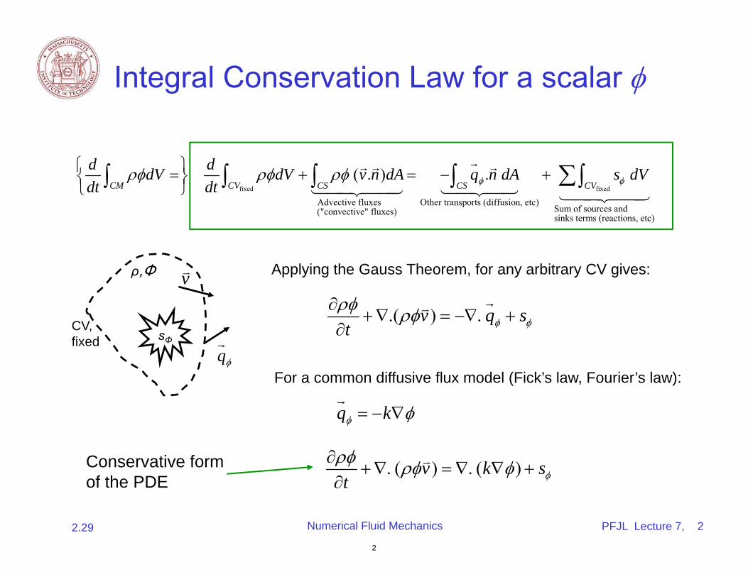
Integral Conservation Law for a scalar

d dV dt CM fixed fixed

Advective fluxes Other transports (diffusion, etc) Sum of sources and ("convective" fluxes) sinks terms (reactions, et

( . ) . CV CS CS CV

d dV v n dA q n dA s dV dt

c)

CV, fixed sΦ

ρ,Φ v Applying the Gauss Theorem, for any arbitrary CV gives:

.(v) . q s t

q

For a common diffusive flux model (Fick’s law, Fourier’s law): q k

Conservative form . (v) . ( k) s of the PDE t


2

ong conservative

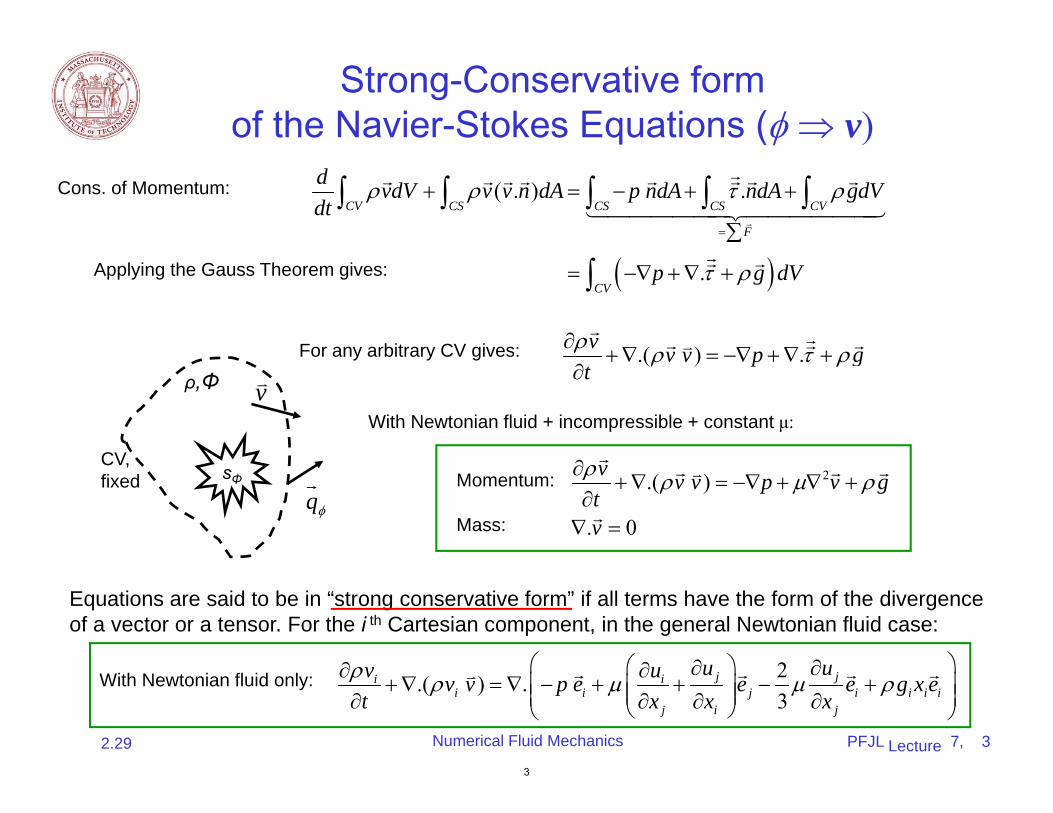
Strong-Conservative formof the Navier-Stokes Equations ( v)

d Cons. of Momentum: vdV v v n dA ( . ) p ndA .ndA gdV CV CS CS CS CVdt

F

Applying the Gauss Theorem gives: p . g dVCV

v For any arbitrary CV gives: .( v v) . g p t

With Newtonian fluid + incompressible + constant μ:

CV, fixed sΦ

ρ,Φ v

v

Momentum: .(v v ) p 2v gtq Mass: .v 0

Numerical Fluid Mechanics PFJL Lecture 7, 32.29

Equations are said to be in “str form” if all terms have the form of the divergence of a vector or a tensor. For the i th Cartesian component, in the general Newtonian fluid case:

2.( ) . 3

j ji i i i j i i i i

j i j

u uv u v v p e e e g x e t x x x

With Newtonian fluid only:

3

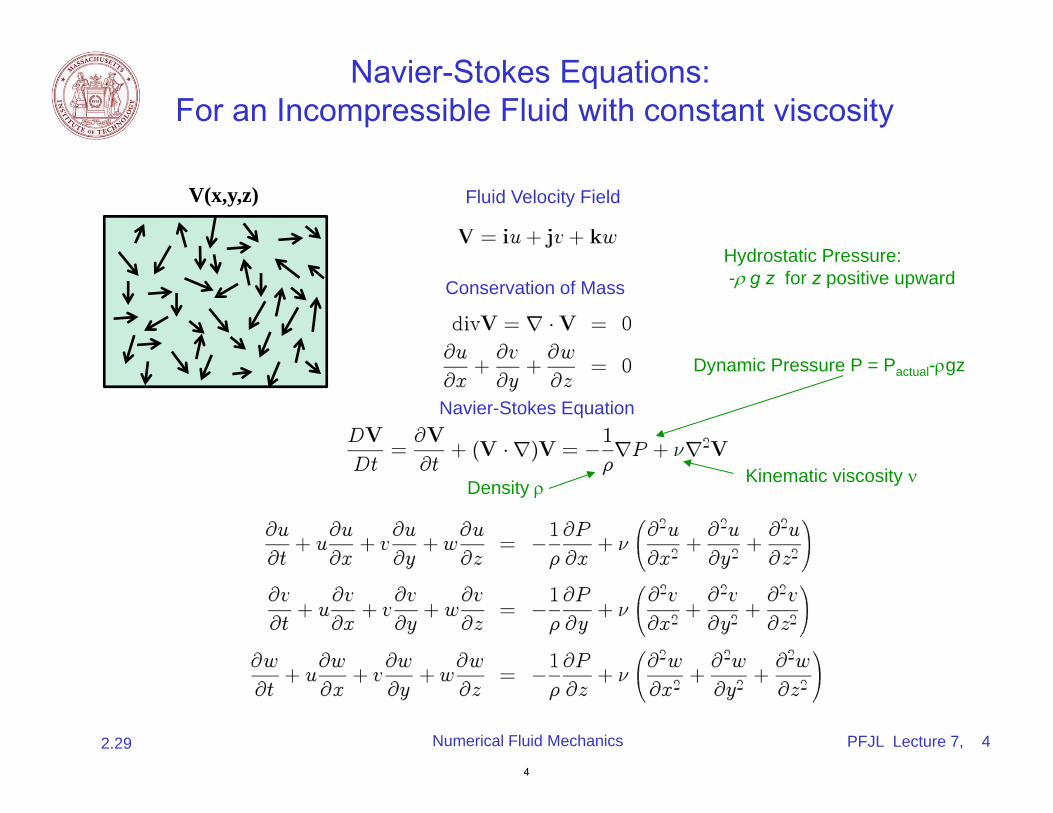
Navier-Stokes Equations:For an Incompressible Fluid with constant viscosity

V(x,y,z) Fluid Velocity Field

Navier-Stokes Equation

Conservation of Mass

Dynamic Pressure P = Pactual -gz

Kinematic viscosity Density

Hydrostatic Pressure: -g z for z positive upward


4

V=

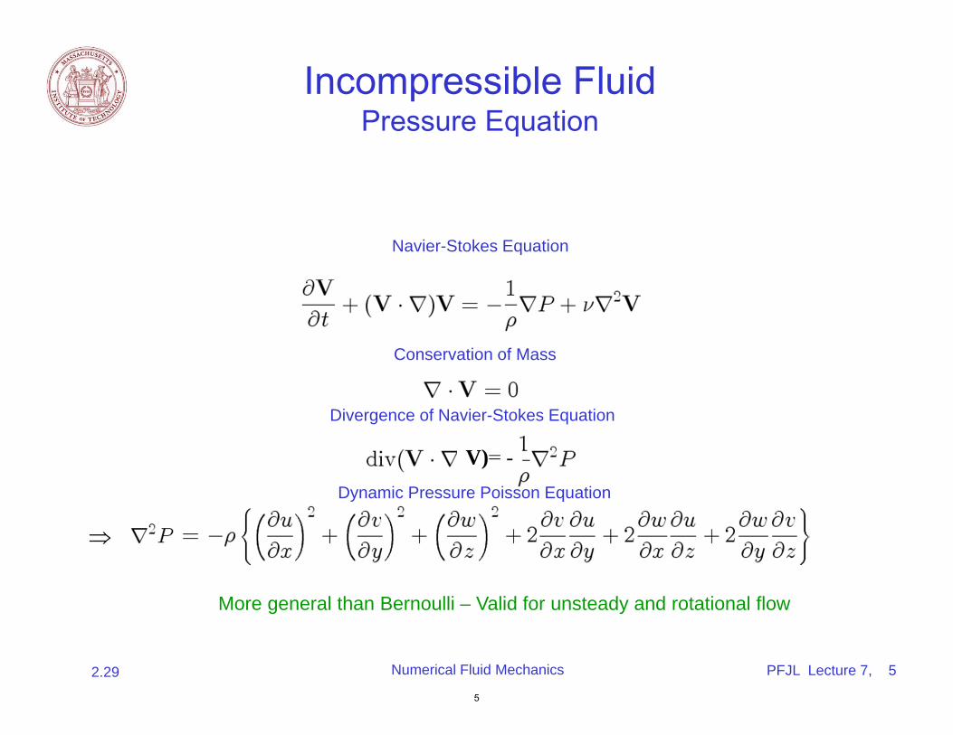
Incompressible FluidPressure Equation



Divergence of Navier-Stokes Equation

Dynamic Pressure Poisson Equation

V)= -

More general than Bernoulli – Valid for unsteady and rotational flow


5

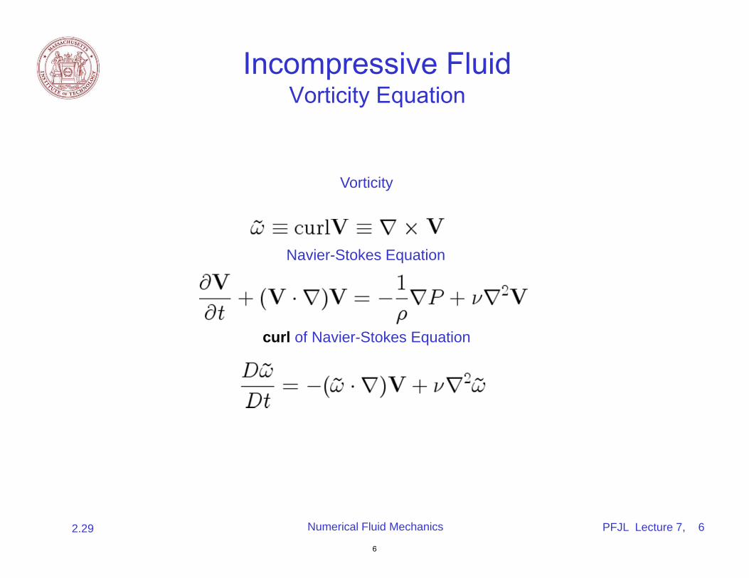
Incompressive FluidVorticity Equation

Vorticity


curl of Navier-Stokes Equation


6

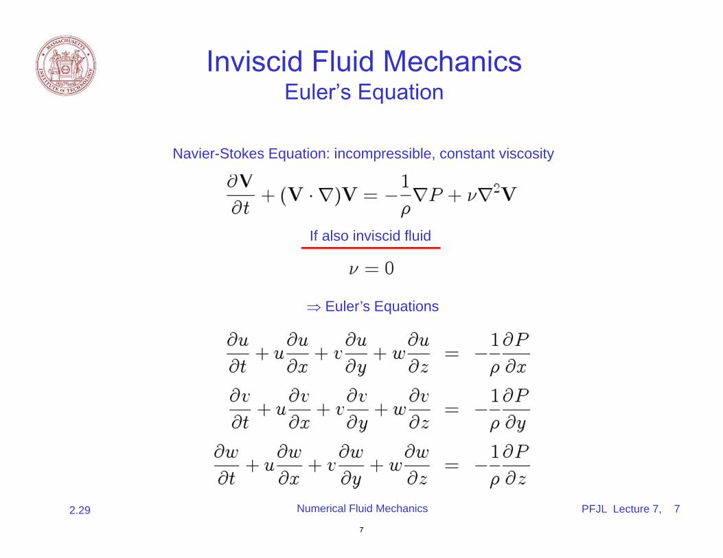
Inviscid Fluid MechanicsEuler’s Equation

Navier-Stokes Equation: incompressible, constant viscosity

If also inviscid fluid

Euler’s Equations


7

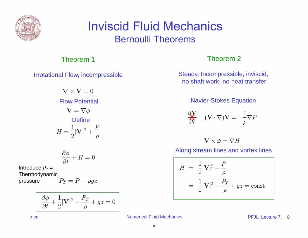
Inviscid Fluid MechanicsBernoulli Theorems

Theorem 1 Theorem 2

Irrotational Flow, incompressible Steady, Incompressible, inviscid, no shaft work, no heat transfer

Flow Potential

Define

Introduce PT = Thermodynamic


pressure

X

Along stream lines and vortex lines


8

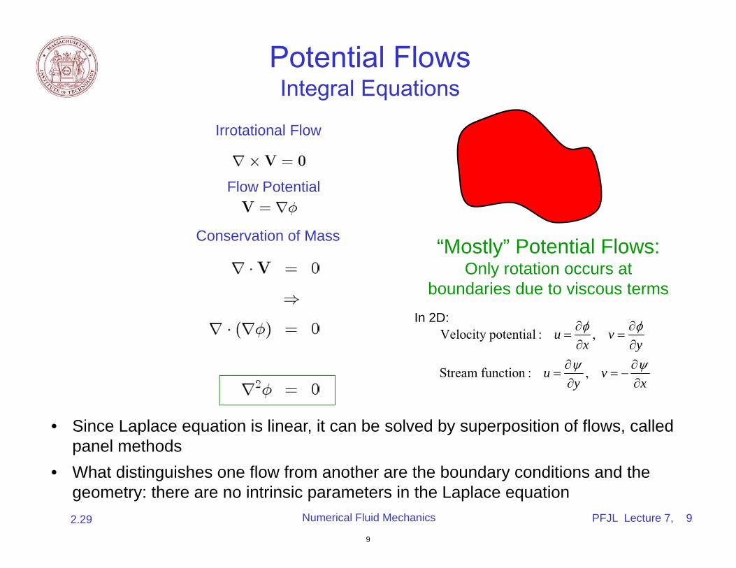
Potential FlowsIntegral Equations

Irrotational Flow

Flow Potential


Laplace Equation

“Mostly” Potential Flows: Only rotation occurs at

boundaries due to viscous terms

In 2D: Velocity potential : u , v x y

Stream function : u , v y x

• Since Laplace equation is linear, it can be solved by superposition of flows, called panel methods

• What distinguishes one flow from another are the boundary conditions and the geometry: there are no intrinsic parameters in the Laplace equation


9

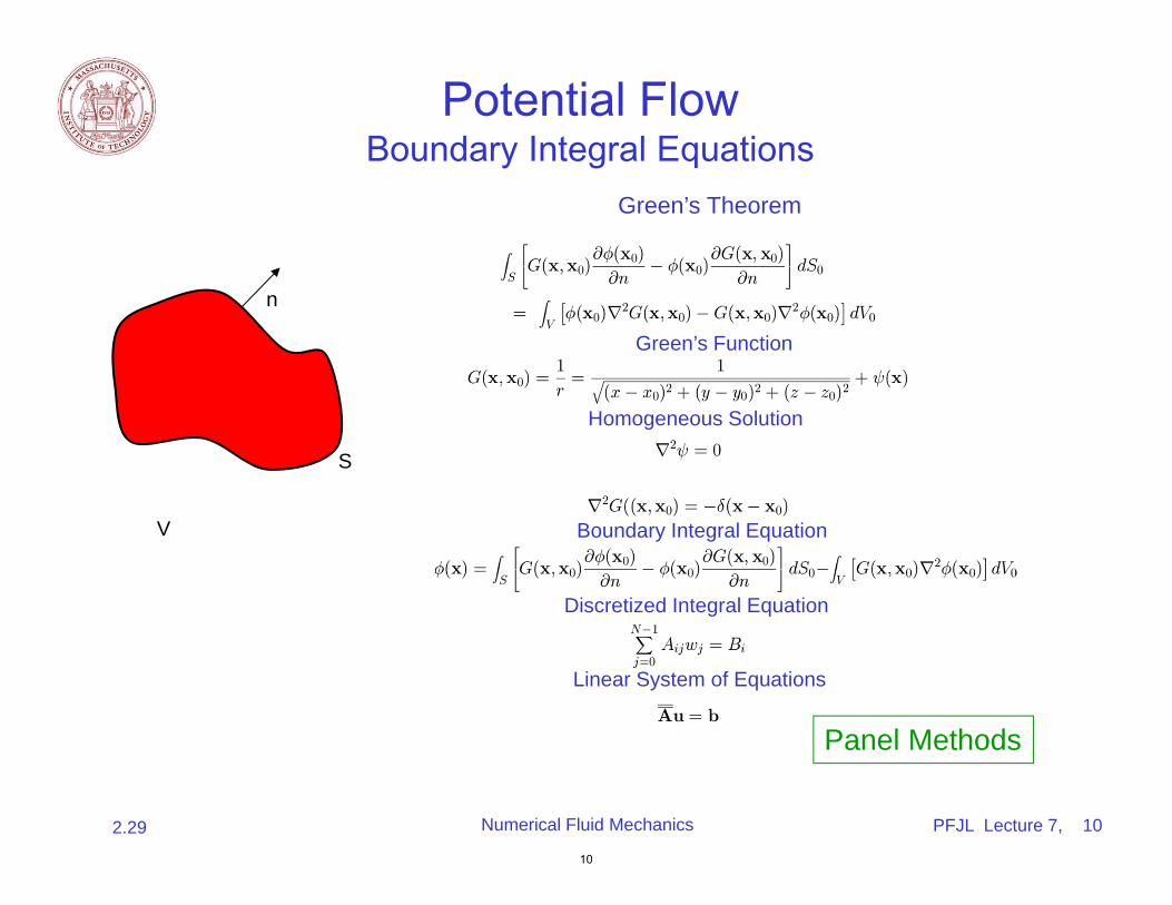
Potential FlowBoundary Integral Equations

Green’s Theorem

S

n

V

Green’s Function

Homogeneous Solution

Boundary Integral Equation

Discretized Integral Equation

Linear System of Equations

Panel Methods

Numerical Fluid Mechanics PFJL Lecture 7, 10

10

2.29

Systems of Linear Equations • Motivation and Plans • Direct Methods for solving Linear Equation Systems

– Cramer’s Rule (and other methods for a small number of equations) – Gaussian Elimination – Numerical implementation

• Numerical stability – Partial Pivoting – Equilibration – Full Pivoting

• Multiple right hand sides, Computation count • LU factorization • Error Analysis for Linear Systems

– Condition Number • Special Matrices: Tri-diagonal systems

• Iterative Methods – Jacobi’s method – Gauss-Seidel iteration

2.29 – Convergence Numerical Fluid Mechanics PFJL Lecture 7, 11

11

Motivations and Plans

• Fundamental equations in engineering are conservation laws (mass, momentum, energy, mass ratios/concentrations, etc)– Can be written as “ System Behavior (state variables) = forcing ”

• Result of the discretized (volume or differential form) of the Navier-Stokes equations (or most other differential equations): – System of (mostly coupled) algebraic equations which are linear or

nonlinear, depending on the nature of the continuous equations

– Often, resulting matrices are sparse (e.g. banded and/or block matrices) • Lectures 3 and 4:

– Methods for solving f(x)=0 or

f(x)=0 f ( ), f x ( ) b– To be used for systems of equations: f(x)=b, i.e: f x ( ),..., f x 1 2 n

• Here we first deal with solving Linear Algebraic equations:

A x b or A X B Numerical Fluid Mechanics PFJL Lecture 7, 12

12

2.29

Motivations and Plans

• Above 75% of engineering/scientific problems involve solving linear systems of equations – As soon as methods were used on computers => dramatic advances

• Main Goal: Learn methods to solve systems of linear algebraic equations and apply them to CFD applications

• Reading Assignment – Part III and Chapter 9 of “Chapra and Canale, Numerical Methods for

Engineers, 2006.” – For Matrix background, see Chapra and Canale (pg 219-227) and

other linear algebra texts (e.g. Trefethen and Bau, 1997) • Other References :

– Any chapter on “Solving linear systems of equations” in CFD references provided.

– For example: chapter 5 of “J. H. Ferziger and M. Peric, Computational Methods for Fluid Dynamics. Springer, NY, 3rd edition, 2002”


13

2.29

Direct Numerical Methodsfor Linear Equation Systems

A x b or A X B

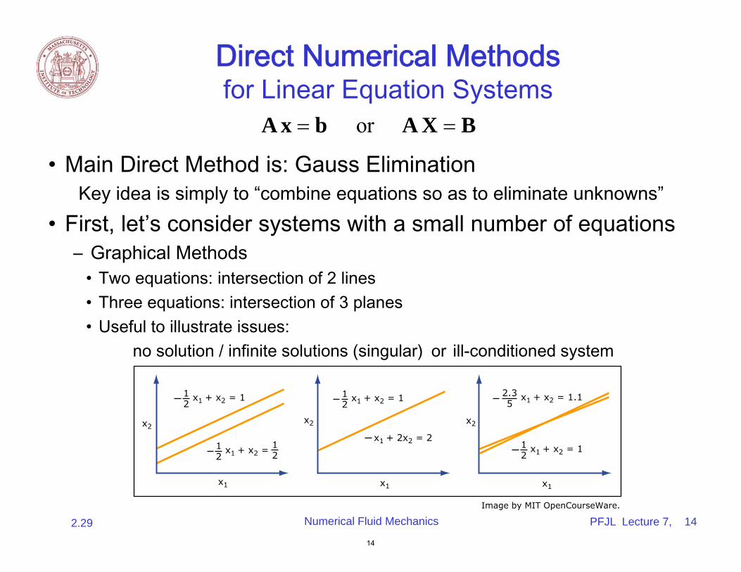
• Main Direct Method is: Gauss Elimination Key idea is simply to “combine equations so as to eliminate unknowns”

• First, let’s consider systems with a small number of equations– Graphical Methods

• Two equations: intersection of 2 lines • Three equations: intersection of 3 planes • Useful to illustrate issues:

no solution / infinite solutions (singular) or ill-conditioned system


14

2.29

12

x1 + x2 = 1 12

x1 + x2 = 1

12

x1 + x2 = 112

12x1 + x2 =

2.35

x1 + x2 = 1.1

x1 + 2x2 = 2x2

x1

x2

x1

x2

x1

Image by MIT OpenCourseWare.

Direct Methods for Small Systems: Determinants and Cramer’s Rule

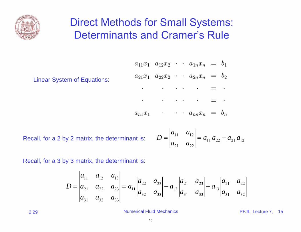
Linear System of Equations:

a a11 12 a a a aRecall, for a 2 by 2 matrix, the determinant is: D 11 22 21 12a a21 22

Recall, for a 3 by 3 matrix, the determinant is:

a a a11 12 13 a a a a a a22 23 21 23 21 22D a a a a11 a12 a13 21 22 23 a a a a a a32 33 31 33 31 32a a a31 32 33


15

2.29

Direct Methods for small systems: Determinants and Cramer’s Rule

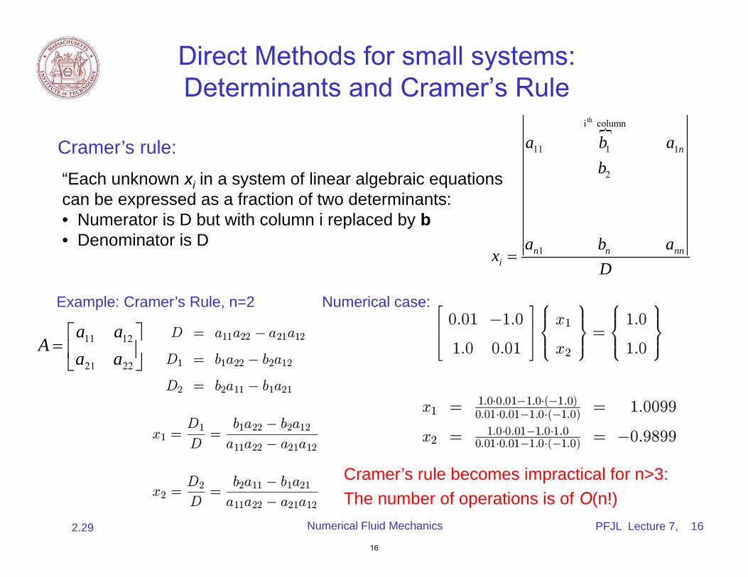
Cramer’s rule: “Each unknown xi in a system of linear algebraic equations can be expressed as a fraction of two determinants: • Numerator is D but with column i replaced by b • Denominator is D

xi

Example: Cramer’s Rule, n=2 Numerical case:

a a11 12A a a 21 22

i column th a b a11 1 1n

b2

a b an1 n nn

D

Cramer’s rule becomes impractical for n>3: The number of operations is of O(n!)


16

2.29

Direct Methods for large dense systems Gauss Elimination

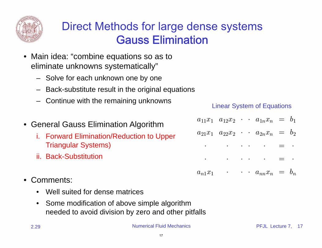
• Main idea: “combine equations so as to eliminate unknowns systematically”

– Solve for each unknown one by one – Back-substitute result in the original equations – Continue with the remaining unknowns

Linear System of Equations

• General Gauss Elimination Algorithm i. Forward Elimination/Reduction to Upper

Triangular Systems) ii. Back-Substitution

• Comments: • Well suited for dense matrices • Some modification of above simple algorithm

needed to avoid division by zero and other pitfalls


17

2.29

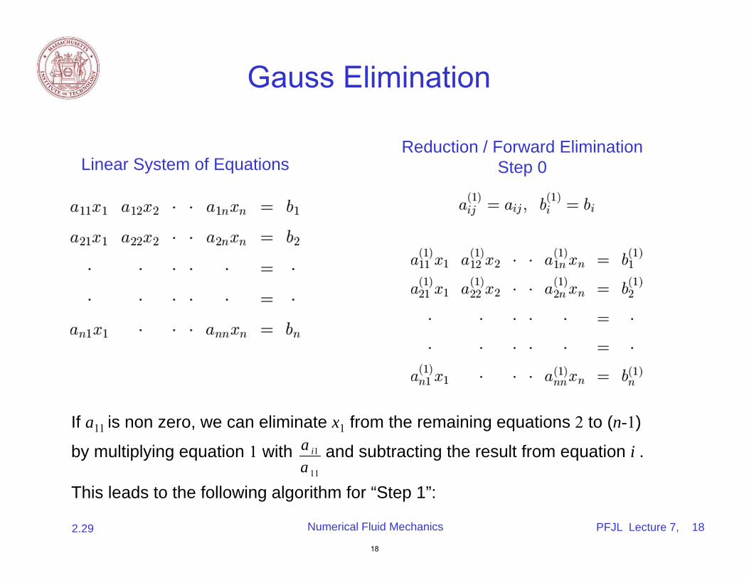
Gauss Elimination

Reduction / Forward Elimination Linear System of Equations Step 0

If a11 is non zero, we can eliminate x1 from the remaining equations 2 to (n-1) a i1by multiplying equation 1 with and subtracting the result from equation i . a 11

This leads to the following algorithm for “Step 1”:


18

2.29

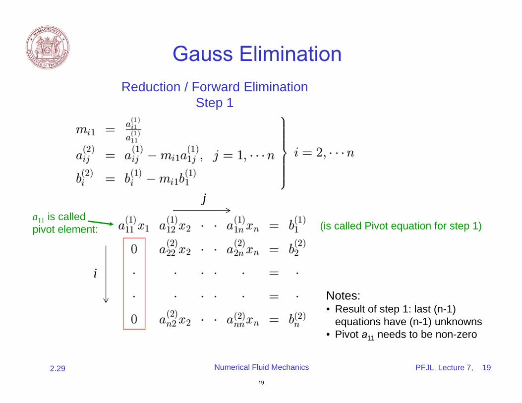
i

j a11 is called pivot element:

Notes:

Gauss Elimination

Reduction / Forward Elimination Step 1

(is called Pivot equation for step 1)

• Result of step 1: last (n-1) equations have (n-1) unknowns

• Pivot a11 needs to be non-zero


19

2.29

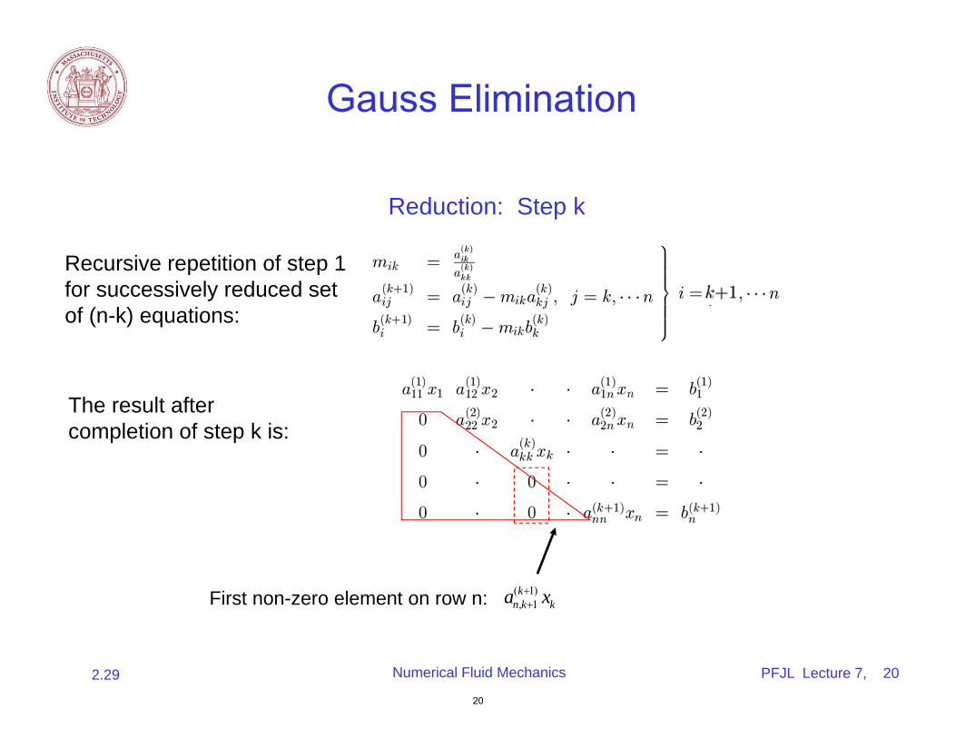
Gauss Elimination

Reduction: Step k

Recursive repetition of step 1 for successively reduced set of (n-k) equations:

The result after completion of step k is:

( 1) kFirst non-zero element on row n: an k, 1 xk


20

2.29

Gauss Elimination

Reduction/Elimination: Step k

Back-Substitution Reduction: Step (n-1)

Result after step (n-1) is an Upper triangular system!


21

2.29

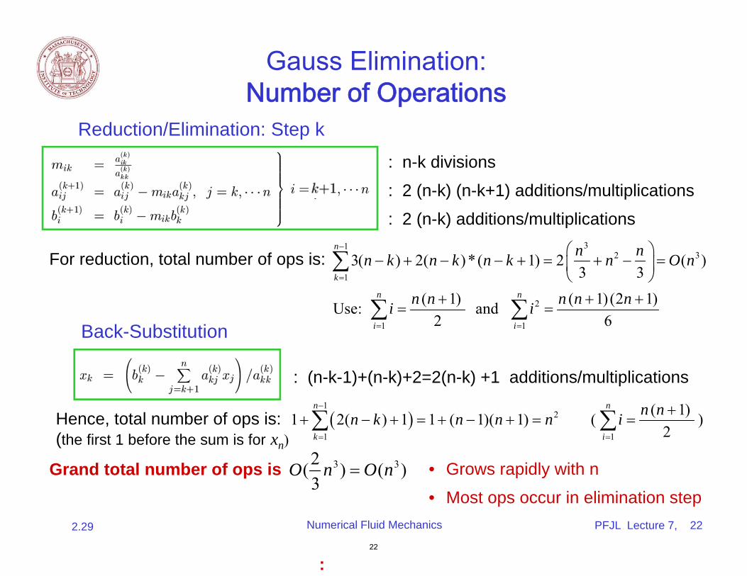
Gauss Elimination: Number of Operations

Reduction/Elimination: Step k

: n-k divisions

: 2 (n-k) (n-k+1) additions/multiplications

: 2 (n-k) additions/multiplications n1 3 n 2 n 3For reduction, total number of ops is: 3(n k) 2( n k)*( n k 1) 2 n O n ( ) k 1 3 3

n ( 1) n 2 n n( 1)(2 n n n 1) Use: i and i

i1 2 i1 6Back-Substitution

: (n-k-1)+(n-k)+2=2(n-k) +1 additions/multiplications n1 n

2 ( 1) n nHence, total number of ops is: 12( n k) 1 1 (n 1)( n 1) n ( i ) k 1 i1(the first 1 before the sum is for xn) 2 3 3( ( • Grows rapidly with n Grand total number of ops is O n ) O n )

:

3• Most ops occur in elimination step


22

2.29

2

Gauss Elimination: Issues and Pitfalls to be addressed

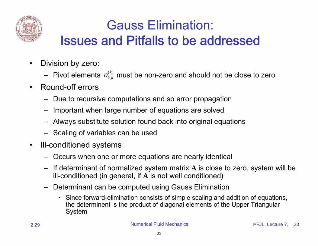
• Division by zero: ( )– Pivot elements k must be non-zero and should not be close to zero , ak k

• Round-off errors – Due to recursive computations and so error propagation – Important when large number of equations are solved – Always substitute solution found back into original equations – Scaling of variables can be used

• Ill-conditioned systems – Occurs when one or more equations are nearly identical – If determinant of normalized system matrix A is close to zero, system will be

ill-conditioned (in general, if A is not well conditioned) – Determinant can be computed using Gauss Elimination

• Since forward-elimination consists of simple scaling and addition of equations, the determinent is the product of diagonal elements of the Upper Triangular System


23

2.29

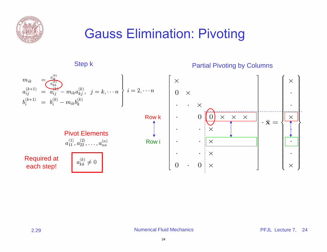
Gauss Elimination: Pivoting

Step k Partial Pivoting by Columns

Row k

Row i Pivot Elements

Required at each step!


24

2.29

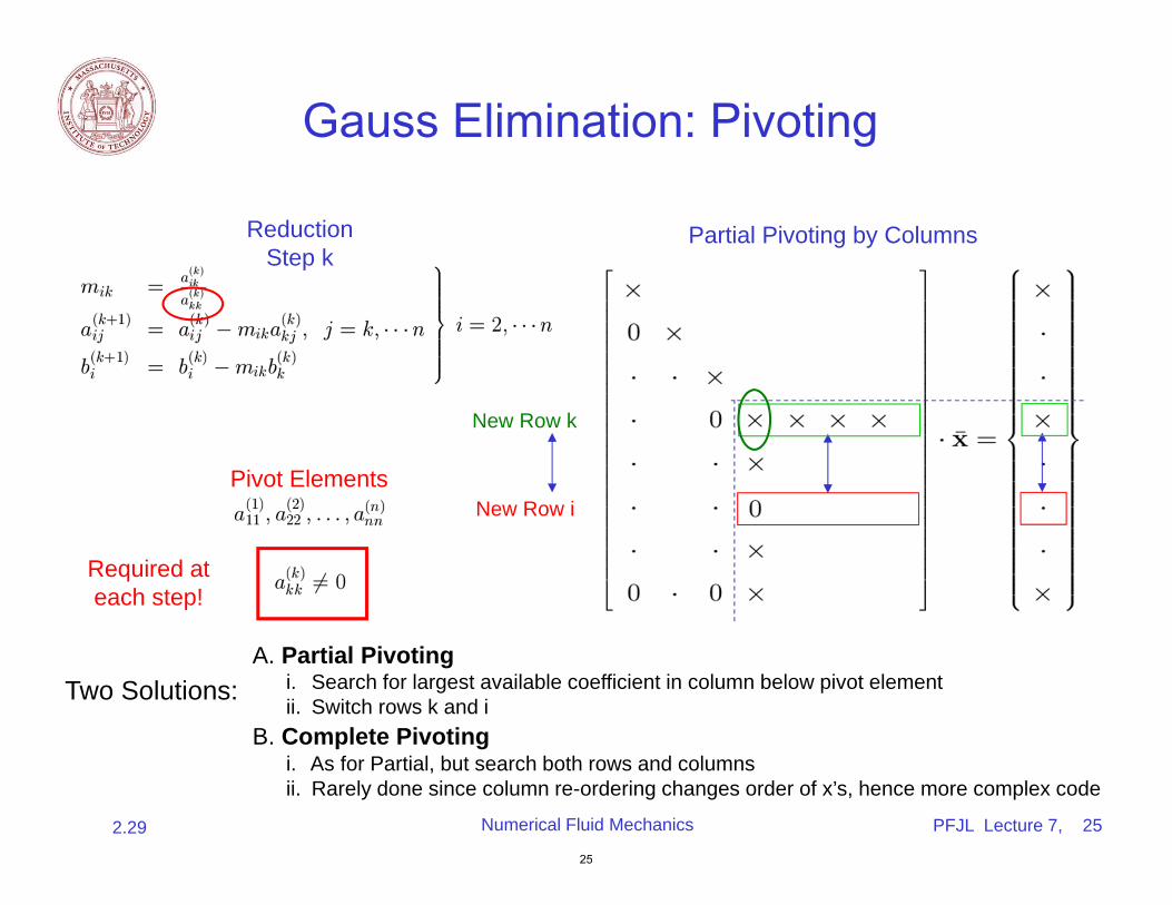
Gauss Elimination: Pivoting

Reduction Partial Pivoting by ColumnsStep k

New Row k

Pivot Elements New Row i

Required at each step!

A. Partial Pivoting i. Search for largest available coefficient in column below pivot element Two Solutions: ii. Switch rows k and i

B. Complete Pivoting i. As for Partial, but search both rows and columns ii. Rarely done since column re-ordering changes order of x’s, hence more complex code


25

2.29

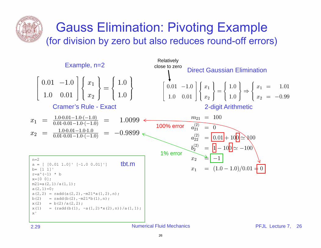
Gauss Elimination: Pivoting Example (for division by zero but also reduces round-off errors)

RelativelyExample, n=2 close to zero Direct Gaussian Elimination

Cramer’s Rule - Exact

n=2 a = [ [0.01 1.0]' [-1.0 0.01]'] tbt.m b= [1 1]'r=a^(-1) * bx=[0 0];m21=a(2,1)/a(1,1);a(2,1)=0;a(2,2) = radd(a(2,2),-m21*a(1,2),n);b(2) = radd(b(2),-m21*b(1),n);x(2) = b(2)/a(2,2);x(1) = (radd(b(1), -a(1,2)*x(2),n))/a(1,1);x'

2-digit Arithmetic

1% error

100% error


26

2.29

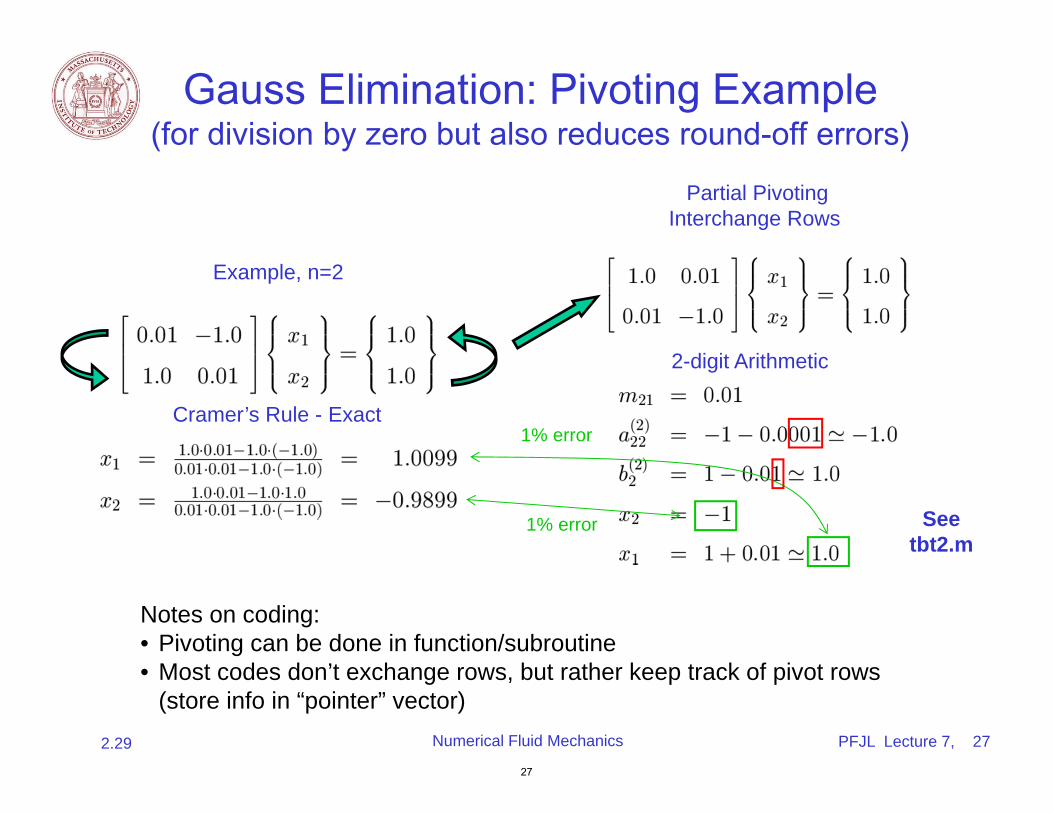
Gauss Elimination: Pivoting Example (for division by zero but also reduces round-off errors)

Partial Pivoting Interchange Rows

Example, n=2


2-digit Arithmetic

1% error

1% error

See tbt2.m

Notes on coding: • Pivoting can be done in function/subroutine • Most codes don’t exchange rows, but rather keep track of pivot rows

(store info in “pointer” vector) Numerical Fluid Mechanics PFJL Lecture 7, 27

27

2.29

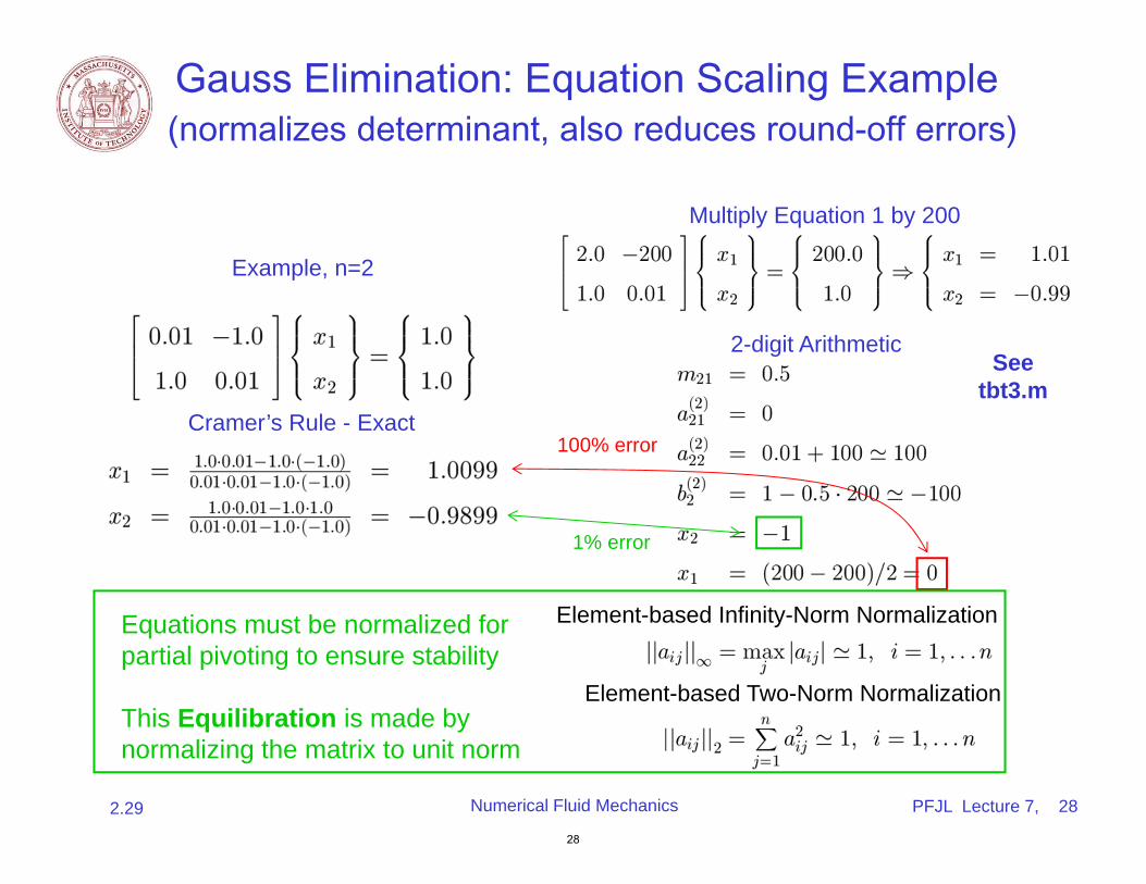
Gauss Elimination: Equation Scaling Example(normalizes determinant, also reduces round-off errors)

Multiply Equation 1 by 200

Example, n=2


2-digit Arithmetic

1% error

100% error

Element-based Infinity-Norm NormalizationEquations must be normalized for partial pivoting to ensure stability

This Equilibration is made by normalizing the matrix to unit norm

Element-based Two-Norm Normalization

See tbt3.m


28

2.29

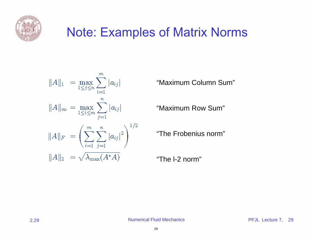
Note: Examples of Matrix Norms

“Maximum Column Sum”

“Maximum Row Sum”

“The Frobenius norm”

“The l-2 norm”


29

2.29

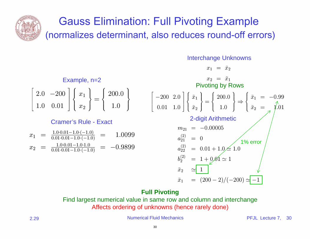
Gauss Elimination: Full Pivoting Example(normalizes determinant, also reduces round-off errors)

Interchange Unknowns

Example, n=2

Cramer’s Rule - Exact 2-digit Arithmetic

1% error

Pivoting by Rows

Full Pivoting Find largest numerical value in same row and column and interchange

Affects ordering of unknowns (hence rarely done) Numerical Fluid Mechanics PFJL Lecture 7, 30

30

2.29

Gauss EliminationNumerical Stability

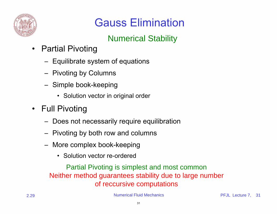
• Partial Pivoting – Equilibrate system of equations – Pivoting by Columns – Simple book-keeping

• Solution vector in original order

• Full Pivoting – Does not necessarily require equilibration – Pivoting by both row and columns – More complex book-keeping

• Solution vector re-ordered

Partial Pivoting is simplest and most common Neither method guarantees stability due to large number

of reccursive computations Numerical Fluid Mechanics PFJL Lecture 7, 31

31

2.29

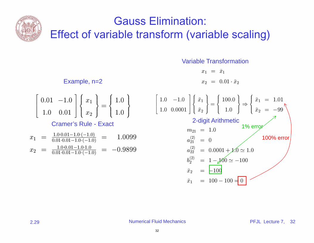
Gauss Elimination: Effect of variable transform (variable scaling)

Variable Transformation

Example, n=2

Cramer’s Rule - Exact 2-digit Arithmetic 1% error

100% error


32

2.29

Systems of Linear EquationsGauss Elimination

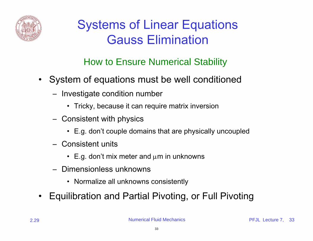
How to Ensure Numerical Stability

• System of equations must be well conditioned – Investigate condition number

• Tricky, because it can require matrix inversion

– Consistent with physics • E.g. don’t couple domains that are physically uncoupled

– Consistent units • E.g. don’t mix meter and m in unknowns

– Dimensionless unknowns • Normalize all unknowns consistently

• Equilibration and Partial Pivoting, or Full Pivoting


33

2.29

MIT OpenCourseWarehttp://ocw.mit.edu

2.29 Numerical Fluid Mechanics Fall 2011

For information about citing these materials or our Terms of Use, visit: http://ocw.mit.edu/terms.

http://ocw.mit.edu

http://ocw.mit.edu/terms

Documents

2.29 Numerical Fluid Mechanics Fall 2011 – Lecture 7€¦ · 2.29 Numerical Fluid Mechanics Fall 2011 – Lecture 7 REVIEW of Lecture 6 Material covered in class: Differential forms