2322 IEEE TRANSACTIONS ON IMAGE …staff.utia.cas.cz/sroubekf/papers/TIP_07.pdf2322 IEEE TRANSACTIONS ON IMAGE PROCESSING, VOL. 16, NO. 9, SEPTEMBER 2007 A Uniﬁed Approach to Superresolution

2322 IEEE TRANSACTIONS ON IMAGE PROCESSING, VOL. 16, NO. 9, SEPTEMBER 2007

A Unified Approach to Superresolutionand Multichannel Blind Deconvolution

Filip Sroubek, Gabriel Cristóbal, Senior Member, IEEE, and Jan Flusser, Senior Member, IEEE

Abstract—This paper presents a new approach to the blinddeconvolution and superresolution problem of multiple degradedlow-resolution frames of the original scene. We do not assume anyprior information about the shape of degradation blurs. The pro-posed approach consists of building a regularized energy functionand minimizing it with respect to the original image and blurs,where regularization is carried out in both the image and blurdomains. The image regularization based on variational principlesmaintains stable performance under severe noise corruption.The blur regularization guarantees consistency of the solutionby exploiting differences among the acquired low-resolutionimages. Several experiments on synthetic and real data illustratethe robustness and utilization of the proposed technique in realapplications.

Index Terms—Image restoration, multichannel blind deconvo-lution, regularized energy minimization, resolution enhancement,superresolution.

I. INTRODUCTION

IMAGING devices have limited achievable resolution due tomany theoretical and practical restrictions. An original scene

with a continuous intensity function warps at the cameralens because of the scene motion and/or change of the cameraposition. In addition, several external effects blur images: at-mospheric turbulence, camera lens, relative camera-scene mo-tion, etc. We will call these effects volatile blurs to emphasizetheir unpredictable and transitory behavior, yet we will assumethat we can model them as convolution with an unknown pointspread function (PSF) . This is a reasonable assumptionif the original scene is flat and perpendicular to the optical axis.Finally, the CCD discretizes the images and produces digitizednoisy image (frame). We refer to as a low-resolu-tion (LR) image, since the spatial resolution is too low to captureall the details of the original scene. In conclusion, the acquisi-tion model becomes

(1)

Manuscript received October 30, 2006; revised May 23, 2007. This work wassupported in part by the Czech Ministry of Education under the project 1M0572(Research Center DAR), in part by the Academy of Sciences of the Czech Re-public under the project AV0Z10750506-I055, in part by the bilateral project2004CZ0009, and in part by the projects TEC2004-00834, TEC2005-24739-E,and PI040765. The associate editor coordinating the review of this manuscriptand approving it for publication was Dr. Tamas Sziranyi.

F. Sroubek and J. Flusser are with the Institute of Information Theory and Au-tomation, Academy of Sciences of the Czech Republic, Pod Vodárenskou vezí 4,18208 Prague 8, Czech Republic (e-mail: [email protected]; [email protected]).

G. Cristóbal is with the Instituto de Óptica, CSIC, Serrano 121, 28006Madrid, Spain (e-mail: [email protected]).

Color versions of one or more of the figures in this paper are available onlineat http://ieeexplore.ieee.org.

Digital Object Identifier 10.1109/TIP.2007.903256

where is additive noise and denotes the geometric de-formation (warping). is the decimation operatorthat models the function of the CCD sensors. It consists of con-volution with the sensor PSF followed by the samplingoperator , which we define as multiplication by a sum of deltafunctions placed on a evenly spaced grid. The above model forone single observation is extremely ill-posed. Instead oftaking a single image we can take images of theoriginal scene and this way partially overcome the equivocationof the problem. Hence, we write

(2)

where , and remains the same in all the acqui-sitions. In the perspective of this multiframe model, the orig-inal scene is a single input and the acquired LR im-ages are multiple outputs. The model is, therefore, calleda single-input–multiple-output (SIMO) formation model. Theupper part of Fig. 1 summarizes the multiframe LR acquisitionprocess. To our knowledge, this is the most accurate, state-of-the-art model, as it takes all possible degradations into account.Several other authors, such as in [1]–[4], adopt this model, aswell.

Superresolution (SR) is the process of combining a sequenceof LR images in order to produce a higher resolution imageor sequence. It is unrealistic to assume that the superresolvedimage can recover the original scene exactly. A rea-sonable goal of SR is a discrete version of that has ahigher spatial resolution than the resolution of the LR imagesand that is free of the volatile blurs (deconvolved). In the paper,we will refer to this superresolved image as a high resolution(HR) image . The standard SR approach consists of sub-pixel registration, overlaying the LR images on an HR grid, andinterpolating the missing values. The subpixel shift between im-ages thus constitutes the essential assumption. We will demon-strate that assuming volatile blurs in the model explicitly bringsabout a more general and robust technique, with the subpixelshift being a special case thereof.

The acquisition model in (2) embraces three distinct casesfrequently encountered in literature. First, if we want to resolvethe geometric degradation , we face a registration problem.Second, if the decimation operator and the geometrictransform are not considered, we face a multichannel (ormultiframe) blind deconvolution (MBD) problem. Third, if thevolatile blur is not considered or assumed known, andis suppressed up to a subpixel translation, we obtain a classicalSR formulation. In practice, it is crucial to consider all threecases at once. We are then confronted with a problem of blindsuperresolution (BSR), which is the subject of this investiga-

1057-7149/$25.00 © 2007 IEEE

SROUBEK et al.: UNIFIED APPROACH TO SUPERRESOLUTION AND MULTICHANNEL BLIND DECONVOLUTION 2323

Fig. 1. (Top) Low-resolution acquisition and (bottom) reconstruction flow.

tion. The approach presented in this manuscript is one of thefirst attempts to solve BSR with only little prior knowledge.

Proper registration techniques can suppress large and com-plex geometric distortions (usually just up to a small between-image shift). There have been hundreds of methods proposed;see, e.g., [5] for a survey. In the rest of this paper, we will as-sume that the LR images are roughly registered and that sreduce to small translations.

The MBD problem has recently attracted considerable atten-tion. First blind deconvolution attempts were based on single-channel formulations, such as in [6]–[9]. Kundur et al. [10], [11]provide a good overview. The problem is extremely ill-posedin the single-channel framework and cannot be resolved in afully blind form. These methods do not exploit the potential ofthe multichannel framework, because in the single-channel casemissing information about the original image in one channelis not supplemented by information in the other channels. Re-search on intrinsically multichannel methods has begun fairlyrecently; refer to [12]–[16] for a survey and other references.Such MBD methods overpass the limitations of previous tech-niques and can recover the blurring functions from the degradedimages alone. We further developed the MBD theory in [17]by proposing a blind deconvolution method for images, whichmight be mutually shifted by unknown vectors. To make thisbrief survey complete, we should not forget to mention a verychallenging problem of shift-variant blind deconvolution, thatwas considered in [18] and [19].

A countless number of papers address the standard SRproblem. A good survey can be found for example in [20] and[21]. Maximum likelihood, maximum a posteriori (MAP), theset theoretic approach using projection on convex sets, andfast Fourier techniques can all provide a solution to the SRproblem. Earlier approaches assumed that subpixel shifts areestimated by other means. More advanced techniques, suchas in [1], [2], and [4], include the shift estimation into the SRprocess. Other approaches focus on fast implementation [3],space-time SR [22] or SR of compressed video [2]. Most ofthe SR techniques assume a priori known blurs. However, inmany cases, such as blurring due to camera motion, the blurcan have a wild shape that is difficult to predict; see examplesof real motion blurs in [23]. Authors in [24]–[26] proposedBSR that can handle parametric PSFs, i.e., PSFs modeled withone parameter. This restriction is unfortunately very limitingfor most real applications. In [27], we extended our MBDmethod to BSR in an intuitive way but one can prove that thisapproach does not estimate PSFs accurately. The same intuitiveapproach was also proposed in [28]. To our knowledge, firstattempts for theoretically correct BSR with an arbitrary PSFappeared in [29] and [30]. The interesting idea proposed thereinis the conversion of the SR problem from SIMO to multipleinput multiple output using so-called polyphase components.We will adopt the same idea here as well. Other preliminaryresults of the BSR problem with focus on fast calculation aregiven in [31], where the authors propose a modification of theRichardson–Lucy algorithm.

Current multiframe blind deconvolution techniques requireno or very little prior information about the blurs, they are suf-ficiently robust to noise and provide satisfying results in mostreal applications. However, they can hardly cope with the deci-mation operator, which violates the standard convolution model.On the contrary, state-of-the-art SR techniques achieve remark-able results of resolution enhancement in the case of no blur.They accurately estimate the subpixel shift between images butlack any apparatus for calculating the blurs.

We propose a unifying method that simultaneously estimatesthe volatile blurs and HR image without any prior knowledgeof the blurs and the original image. We accomplish this by for-mulating the problem as a minimization of a regularized en-ergy function, where the regularization is carried out in boththe image and blur domains. The image regularization is basedon variational integrals, and a consequent anisotropic diffusionwith good edge-preserving capabilities. A typical example ofsuch regularization is total variation first proposed in [32]. How-ever, the main contribution of this work lies in the developmentof the blur regularization term. We show that the blurs can berecovered from the LR images up to small ambiguity. One canconsider this as a generalization of the results proposed for blurestimation in the case of MBD problems. This fundamental ob-servation enables us to build a simple regularization term forthe blurs even in the case of the SR problem. To tackle the mini-mization task, we use an alternating minimization approach (seeFig. 1), consisting of two simple linear equations.

The rest of the paper is organized as follows. Section II out-lines the degradation model. In Section III, we present a pro-cedure for volatile blur estimation. This effortlessly transformsinto a regularization term of the BSR algorithm as describedin Section IV. Finally, Section V illustrates applicability of theproposed method to real situations.


II. MATHEMATICAL MODEL

To simplify the notation, we will assume only images andPSFs with square supports. An extension to rectangular imagesis straightforward. Let be an arbitrary discrete image ofsize , then denotes an image column vector of size

and denotes a matrix that performs convolutionof with an image of size . The convolution matrix canhave a different output size. Adopting the Matlab naming con-vention, we distinguish two cases: “full” convolution ofsize and “valid” convolution of size

. In both cases, the convolution matrix is aToeplitz-block-Toeplitz matrix. We will not specify dimensionsof convolution matrices if it is obvious from the size of the rightargument.

Let us assume we have different LR frames (each ofsize ) that represent degraded (blurred and noisy) versionsof the original scene. Our goal is to estimate the HR represen-tation of the original scene, which we denoted as the HR image

of size . The LR frames are linked with the HR imagethrough a series of degradations similar to those betweenand in (2). First is geometrically warped , then it isconvolved with a volatile PSF and finally it is decimated

. The formation of the LR images in vector-matrix notationis then described as

(3)

where is additive noise present in every channel. The decima-tion matrix simulates the behavior of digital sensorsby first performing convolution with the sensor PSFand then downsampling . The Gaussian function is widelyaccepted as an appropriate sensor PSF and it is also used here. Itsjustification is experimentally verified in [33]. A physical inter-pretation of the sensor blur is that the sensor is of finite size and itintegrates impinging light over its surface. The sensitivity of thesensor is highest in the middle and decreases towards its borderswith a Gaussian-like decay. Further, we assume that the sub-sampling factor (or SR factor, depending on the point of view),denoted by , is the same in both and directions. It is impor-tant to underline that is a user-defined parameter. In principle,

can be a very complex geometric transform that must beestimated by image registration or motion detection techniques.We have to keep in mind that subpixel accuracy in s is nec-essary for SR to work. Standard image registration techniquescan hardly achieve this and they leave a small misalignment be-hind. Therefore, we will assume that complex geometric trans-forms are removed in the preprocessing step and reduces toa small translation. Hence, , where performsconvolution with the shifted version of the volatile PSF , andthe acquisition model becomes

(4)

The BSR problem then adopts the following form: We know theLR images and we want to estimate the HR image forthe given and the sensor blur . To avoid boundary effects,we assume that each observation captures only a part of .Hence, and are “valid” convolution matrices

and , respectively. In general, the PSFs are ofdifferent size. However, we postulate that they all fit into a

support.In the case of , the downsampling is not present

and we face a slightly modified MBD problem that has beensolved elsewhere [12], [17]. Here, we are interested in the caseof , when the downsampling occurs. Can we estimatethe blurs as in the case ? The presence of prevents usfrom using the cited results directly. However, we will show thatconclusions obtained for MBD apply here in a slightly modifiedform, as well.

III. RECONSTRUCTION OF VOLATILE BLURS

Estimation of blurs in the MBD case (no downsampling) at-tracted considerable attention in the past. A wide variety ofmethods were proposed, such as in [12] and [13], that providea satisfactory solution. For these methods to work correctly,certain channel disparity is necessary. The disparity is definedas weak co-primeness of the channel blurs, which states thatthe blurs have no common factor except a scalar constant. Inother words, if the channel blurs can be expressed as a con-volution of two subkernels, then there is no subkernel that iscommon to all blurs. An exact definition of weakly co-primeblurs can be found in [13]. Many practical cases satisfy thechannel co-primeness, since the necessary channel disparity ismostly guaranteed by the nature of the acquisition scheme andrandom processes therein. We refer the reader to [12] for a rele-vant discussion. This channel disparity is also necessary for theBSR case.

Let us first recall how to estimate blurs in the MBD caseand then we will generalize the results for integer downsam-pling factors. For the time being, we will omit noise , untilSection IV, where we will address it appropriately.

A. MBD Case

The decimation matrix is not present in (4) and only convo-lution binds the input with the outputs. The acquisition model isof the SIMO type with one input channel and output chan-nels . Under the assumption of channel co-primeness, we cansee that any two correct blurs and satisfy

(5)

There are such relations and they can be arrangedinto one system. Let us define

.... . .

......

.... . .

... (6)

for , where . The completesystem of relations (5) then takes the form

(7)

where . In most real situations, the correctblur size (we have assumed square size ) is not known


in advance, and, therefore, we can generate the above equationfor different blur dimensions . The nullity (null-spacedimension) of is exactly 1 for the correctly estimatedblur size. By applying SVD (singular value decomposition),we recover precisely the blurs except for a scalar factor. Onecan eliminate this magnitude ambiguity by stipulating that

, which is a common brightness preservingassumption. For the underestimated blur size, the above equa-tion has no solution. If the blur size is overestimated, then

.

B. BSR Case

Before we proceed, it is necessary to define precisely thesampling matrix . Let denote a 1-D sampling matrix, where

is the integer subsampling factor. Each row of the samplingmatrix is a unit vector whose nonzero element is at such positionthat, if the matrix multiplies an arbitrary vector , the result ofthe product is every th element of . If the vector length isthen the size of the sampling matrix is . If is notdivisible by , we can pad the vector with an appropriate numberof zeros to make it divisible. A 2-D sampling matrix is defined by

(8)

where denotes the matrix direct product (Kronecker productoperator). Note that the transposed matrix behaves as anupsampling operator that interlaces the original samples with

zeros.A naive approach, as proposed in [27] and [28], is to modify

(7) for the MBD case by applying downsampling,, and formulating the problem as

(9)

where is the identity matrix. One can easily verifythat the condition in (5) is not satisfied for the BSR case as thepresence of downsampling operators violates the commutativeproperty of convolution. Even more disturbing is the fact thatminimizers of (9) do not have to correspond to the correct blurs.We are going to show that if one uses a slightly different ap-proach, reconstruction of the volatile PSFs is possible evenin the BSR case. However, we will see that some ambiguity inthe solution of is inevitable.

First, we need to rearrange the acquisition model (4) and con-struct from the LR images a convolution matrix with apredetermined nullity. Then, we take the null space of andconstruct a matrix , which will contain the correct PSFs inits null space.

Let be the size of “nullifying” filters . (The meaningof this name will be clear later). Define ,where are “valid” convolution matrices. As-suming no noise, we can express in terms of , , and as

(10)

where(11)

and .

The convolution matrix has more rows than columns, and,therefore, it is of full column rank (see proof in [12] for gen-eral convolution matrices). We assume that has full columnrank as well. This is almost certainly true for real images ifhas at least times more rows than columns. Thus,

and the difference between the number of columns androws of bounds from below the null space dimension, i.e.,

(12)

Setting and , wevisualize the null space as

.... . .

... (13)

where is the vector representation of the nullifying filterof size , and . The filtersare made of values of ’s null space and that is where their

name comes from. Let denote upsampled by factor ,i.e., . Then, we define

.... . .

... (14)

and conclude that

(15)

where . We have arrived to an equation thatis of the same form as (7) in the MBD case. Here, we have thesolution to the blur estimation problem for the BSR case. How-ever, since is involved, ambiguity of the solution is higher.Without proofs (for the sake of simplicity) we provide the fol-lowing statements. For the correct blur size, .For the underestimated blur size, (15) has no solution. For theoverestimated blur size ,

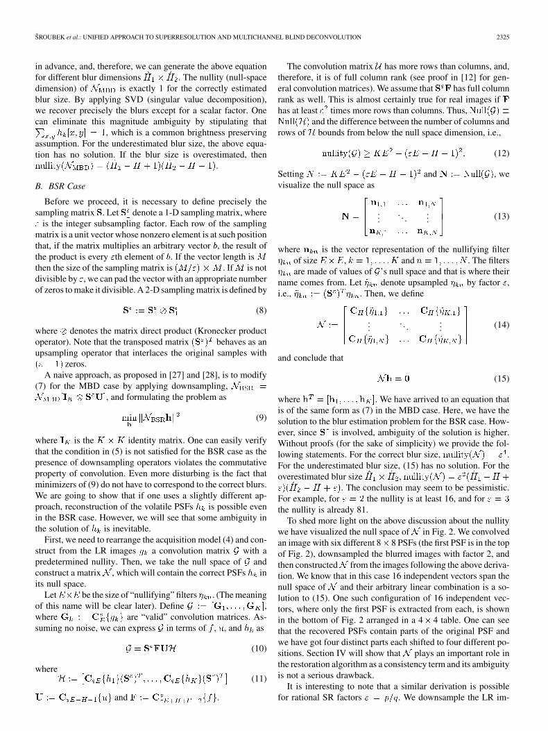
. The conclusion may seem to be pessimistic.For example, for the nullity is at least 16, and forthe nullity is already 81.

To shed more light on the above discussion about the nullitywe have visualized the null space of in Fig. 2. We convolvedan image with six different 8 8 PSFs (the first PSF is in the topof Fig. 2), downsampled the blurred images with factor 2, andthen constructed from the images following the above deriva-tion. We know that in this case 16 independent vectors span thenull space of and their arbitrary linear combination is a so-lution to (15). One such configuration of 16 independent vec-tors, where only the first PSF is extracted from each, is shownin the bottom of Fig. 2 arranged in a 4 4 table. One can seethat the recovered PSFs contain parts of the original PSF andwe have got four distinct parts each shifted to four different po-sitions. Section IV will show that plays an important role inthe restoration algorithm as a consistency term and its ambiguityis not a serious drawback.

It is interesting to note that a similar derivation is possiblefor rational SR factors . We downsample the LR im-


Fig. 2. Visualization of N ’s null space for " = 2. (Top) Original 8� 8 PSFand (bottom) one example of 16 PSFs that span the null space of N . Properlinear combination of these 16 PSFs gives the original PSF.

ages with the factor , thereby creating images and applythereon the above procedure for the SR factor .

Another consequence of the above derivation is the minimumnecessary number of LR images for the blur reconstruction towork. The condition of the nullity in (12) implies that theminimum number is . For example, for 3/2, 3 LRimages are sufficient; for , we need at least 5 LR imagesto perform blur reconstruction. An intuitive explanation is that

input images are necessary for the SR problem to get a fullydetermined system of equations and additional input images arefor the PSF estimation.

IV. BLIND SUPERRESOLUTION

In order to solve the BSR problem, i.e., determine the HRimage and volatile PSFs , we adopt an approach of mini-mizing a regularized energy function. This way, the method willbe less vulnerable to noise and better posed. The energy consistsof three terms and takes the form

(16)

The first term measures the fidelity to the data and emanatesfrom our acquisition model (4). The remaining two are regu-larization terms with positive weighting constants and thatattract the minimum of to an admissible set of solutions. Theform of very much resembles the energy proposed in [17] forMBD. Indeed, this should not come as a surprise since MBDand SR are related problems in our formulation.

Regularization is a smoothing term of the form

(17)

where is a high-pass filter. A common strategy is to use con-volution with the Laplacian for , which in the continuous casecorresponds to . Recently, variational integrals

were proposed, where is a strictly convex,nondecreasing function that grows at most linearly. Examplesof are (total variation), (hypersurface min-imal function), , or nonconvex functions, such as

, and (Mumford–Shah func-tional). The advantage of the variational approach is that it be-haves as anisotropic diffusion. While in smooth areas it has thesame isotropic behavior as the Laplacian, it also preserves edgesin images. The disadvantage is that it is highly nonlinear. Toovercome this difficulty one must use, e.g., the half-quadraticalgorithm [34]. For the purpose of our discussion, it suffices tostate that after discretization we arrive again at (17), where thistime is a positive semidefinite block tridiagonal matrix con-structed of values depending on the gradient of . The rationalebehind the choice of is to constrain the local spatial be-havior of images; it resembles a Markov random field. Someglobal constraints may be more desirable but are difficult (oftenimpossible) to define, since we develop a general method thatshould work with any class of images.

The PSF regularization term directly follows from theconclusions of the previous section. Since the matrix in (14)contains the correct PSFs in its null space, we define theregularization term as a least-squares fit

(18)

If one replaces with , we have the naive approach. Theproduct is a positive semidefinite matrix. More precisely,

is a consistency term that binds volatile PSFs and preventsthem from moving freely and, unlike the fidelity term [the firstterm in (16)], it is based solely on the observed LR images. Agood practice is to include with a small weight a smoothing term

in . This is especially useful in the case of less noisydata in order to overcome the higher nullity of .

The complete energy then takes the form

(19)

Energy as a function of both variables and , is not convexdue to convolution in the first term. On the other hand, the en-ergy function is convex with respect to if is fixed and itis convex with respect to if is fixed. The minimization se-quence can, thus, be built by alternating between twominimization subproblems. This procedure is called alternatingminimizations (AM) and the advantage lies in its simplicity. Foreach subproblem a unique minimum exists that can be easilycalculated. Derivatives w.r.t. and must be zero at the minima,which, in this case, leads to solving a set of simple linear equa-tions. In conclusion, starting with some initial the two itera-tive steps are

Step 1)

(20)

Step 2)

(21)


where , and is the iter-ation step. The AM approach is a variation on the steepest-de-scent algorithm. The search space is a concatenation of the blursubspace and the image subspace. The algorithm first descendsin the image subspace and after reaching the minimum, i.e.,

, it advances in the blur subspace in the directionorthogonal to the previous one, and this scheme repeats.

Due to the coupling of the variables by convolution, we cannotguarantee in theory that the global minimum is reached but thor-ough testing indicates good convergence properties of the algo-rithm for many real problems.

Convergence may further improve if we add feasible regionsfor the HR image and PSFs specified as lower and upper boundsconstraints. To solve step 1, we use the method of conjugategradients (function cgs in standard Matlab) and then adjust thesolution to contain values in the admissible range, typi-cally, the range of values of . It is common to assume thatPSF is positive and preserves image brightness, i.e.,and . We can, therefore, restrict the intensityvalues of PSFs between 0 and 1. In order to enforce the boundsin step 2, we solve (21) as a constrained minimization problem(function fmincon in Matlab Optimization Toolbox v.3) ratherthan using the projection as in step 1. Constrained minimizationproblems are more computationally demanding but we can af-ford it in this case since the size of is much smaller than thesize of .

The weighting constants and depend on the level ofnoise. If noise increases, and should increase, andshould decrease. One can use parameter estimation techniques,such as cross-validation [24] or expectation maximization [35],to determine the correct weights. However, in our experiments,we set the values manually according to a visual assessment.If the iterative algorithm begins to amplify noise, we haveunderestimated the noise level. On the contrary, if the algorithmbegins to segment the image, we have overestimated the noiselevel.

V. EXPERIMENTS

This section consists of two parts. In the first one, a set ofexperiments on synthetic data evaluate performance of the BSRalgorithm with respect to the SR factor and compare the recon-struction quality with other methods mentioned below under dif-ferent levels of noise. The second part demonstrates the appli-cability of the proposed method to real data.

In all the experiments the sensor blur is fixed and set to aGaussian function of standard deviation (relative tothe scale of LR images). One should underline that the proposedBSR method is fairly robust to the choice of the Gaussian vari-ance, since it can compensate for insufficient variance by auto-matically including the missing factor of Gaussian functions inthe volatile blurs.

Another potential pitfall that we have to take into consider-ation is a feasible range of SR factors. Theoretically there areno limitations on the upper bound of the SR factor. However,practical reasons impose limits. As the SR factor increases,we need more LR images . The increasing number ofLR images negatively affects the stability of BSR, since in realscenarios perturbations of the acquisition model occur, which

disrupts the minimization scheme. SR factors beyond 2.5 are,thus, rare in real applications. A more elaborated discussion onfundamental limits of SR algorithms is given in [36]. In addi-tion, rational SR factors , where and are incommensu-rable and large regardless of the effective value of , also makethe BSR algorithm unstable. It is the numerator that deter-mines the internal SR factor used in the algorithm. Hence, welimit ourselves to between 1 and 2.5, such as 3/2, 5/3, 2, etc.,which is sufficient in most practical applications.

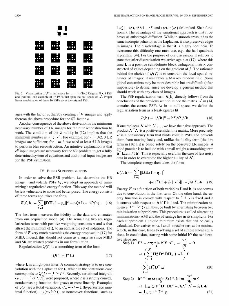
A. Simulated Data

First, let us demonstrate the BSR performance with a simpleexperiment. An 175 175 image in Fig. 3(a) blurred with sixmasks in Fig. 3(b) and downsampled with factor 2 gives six LRimages. Using the LR images as an input, we estimated the orig-inal HR image with the proposed BSR algorithm for and2. Fig. 4 summarizes obtained results in their original size. Onecan see, that for [Fig. 4(b)], the reconstruction is goodbut some details, such as the shirt texture, are still fuzzy. For theSR factor 2, the reconstructed image in Fig. 4(c) is almost per-fect as most of the high-frequency information of the originalimage is correctly recovered.

Next, we evaluate noise robustness of the proposed BSRand compare it with other two methods: interpolation tech-nique and state-of-the-art SR method. The former techniqueconsists of the MBD method proposed in [17] followed bystandard bilinear interpolation resampling. The MBD methodfirst removes volatile blurs and then the interpolation of thedeconvolved image achieves the desired spatial resolution.The latter method, which we will call herein a “standard SRalgorithm,” is a MAP formulation of the SR problem proposed,e.g., in [1] and [2]. This method uses a MAP framework for thejoint estimation of image registration parameters (in our caseonly translation) and the HR image, assuming only the sensorblur and no volatile blurs. For an image prior, we use edgepreserving Huber Markov random fields [33].

In the case of BSR, Section III shows that two distinct ap-proaches exist for the blur estimation. Either we use the naiveapproach in (9) that directly utilizes the MBD formulation, or weapply the intrinsically SR approach given in (15). Depending onthe approach, we use either or in the blur consistencyterm in the AM algorithm.

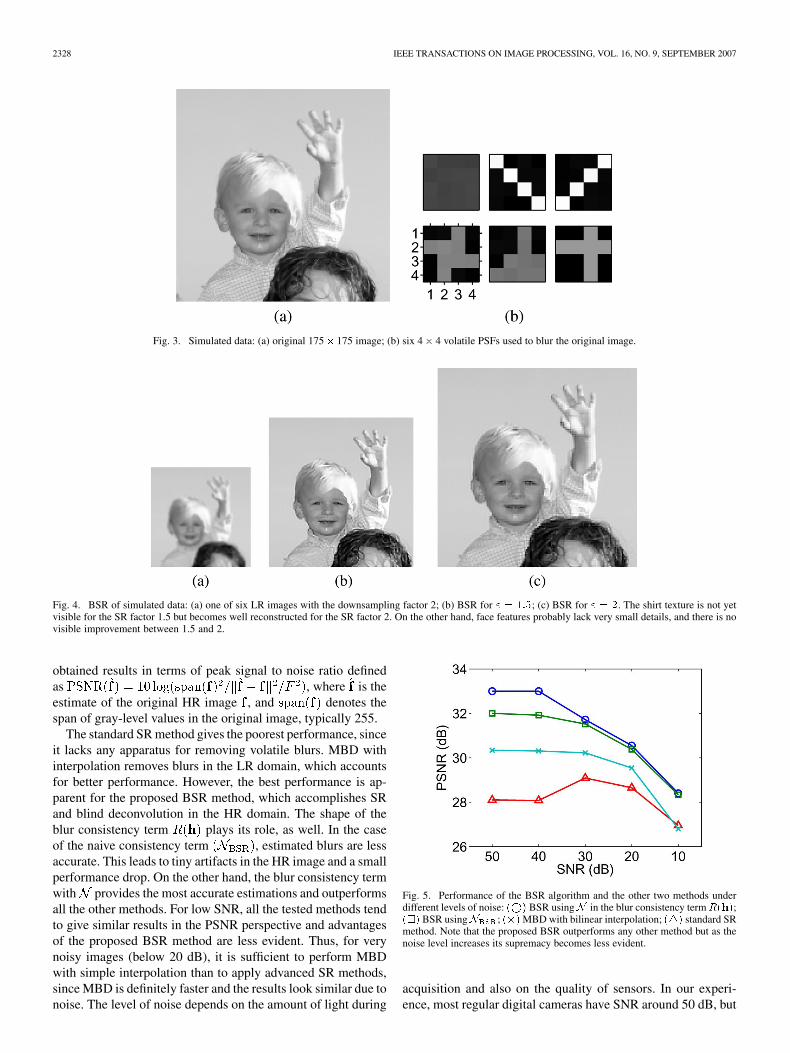
Altogether we have, thus, four distinct methods for com-parison: standard SR approach, MBD with interpolation, BSRwith naive blur regularization and BSR with intrinsic blurregularization. The experimental setup was the following.First, we generated six random motion blurs of size 4 4.Then we generated six LR images from the original HRimage in Fig. 3(a) using the blurs and the downsamplingfactor of 2, and added white Gaussian noise with differentSNR from 50 to 1 dB. The signal-to-noise ratio is defined asSNR , where and are the image andnoise standard deviations, respectively. We repeated the wholeprocedure ten times for different realizations of noise. For eachset of six LR images, the four methods were applied one byone. Parameters of each method were chosen to minimize themean square error of the HR estimate. Fig. 5 summarizes the


Fig. 3. Simulated data: (a) original 175� 175 image; (b) six 4� 4 volatile PSFs used to blur the original image.

Fig. 4. BSR of simulated data: (a) one of six LR images with the downsampling factor 2; (b) BSR for " = 1:5; (c) BSR for " = 2. The shirt texture is not yetvisible for the SR factor 1.5 but becomes well reconstructed for the SR factor 2. On the other hand, face features probably lack very small details, and there is novisible improvement between 1.5 and 2.

obtained results in terms of peak signal to noise ratio definedas , where is theestimate of the original HR image , and denotes thespan of gray-level values in the original image, typically 255.

The standard SR method gives the poorest performance, sinceit lacks any apparatus for removing volatile blurs. MBD withinterpolation removes blurs in the LR domain, which accountsfor better performance. However, the best performance is ap-parent for the proposed BSR method, which accomplishes SRand blind deconvolution in the HR domain. The shape of theblur consistency term plays its role, as well. In the caseof the naive consistency term , estimated blurs are lessaccurate. This leads to tiny artifacts in the HR image and a smallperformance drop. On the other hand, the blur consistency termwith provides the most accurate estimations and outperformsall the other methods. For low SNR, all the tested methods tendto give similar results in the PSNR perspective and advantagesof the proposed BSR method are less evident. Thus, for verynoisy images (below 20 dB), it is sufficient to perform MBDwith simple interpolation than to apply advanced SR methods,since MBD is definitely faster and the results look similar due tonoise. The level of noise depends on the amount of light during

Fig. 5. Performance of the BSR algorithm and the other two methods underdifferent levels of noise: ( ) BSR usingN in the blur consistency term R(h);( ) BSR usingN ; (�) MBD with bilinear interpolation; (4) standard SRmethod. Note that the proposed BSR outperforms any other method but as thenoise level increases its supremacy becomes less evident.

acquisition and also on the quality of sensors. In our experi-ence, most regular digital cameras have SNR around 50 dB, but


Fig. 6. Reconstruction of images acquired with a camcorder (" = 2:5): (a) eight LR frames created from a short video sequence captured with the camcorderand displayed in their original size; (b) bilinear interpolation of one LR frame; (c) BSR estimate of the HR frame; (d) original HR frame.

Fig. 7. Reconstruction of images acquired with a digital camera (" = 2): (a) eight LR acquired shot with the digital camera and displayed in their original size;(b) bilinear interpolation of one LR image; (c) BSR estimate of the HR image; (d) image taken by the same camera but with optical zoom. The BSR algorithmachieves reconstruction comparable to the image with optical zoom.

with decreasing light, it can drop down to 30 dB. Webcamerashave in general lower SNR around 30 dB, even in moderate lightconditions.

B. Real Data

The next three experimental settings come from a licenseplate recognition task and they demonstrate the true power ofthe BSR algorithm. We used data from two different acquisi-tion devices: camcorder and digital camera. The camcorder wasSony Digital Handycam and the digital camera was 5-MpixelOlympus C5050Z equipped with 3 optical zoom. In order to

work with color images, we extended the proposed BSR methodby utilizing color TV [37] instead of standard TV in image reg-ularization and by assuming the same blurring in all three colorchannels.

In the first scenario, we used a short video sequence pro-vided by Dr. Z. Geradts from the Netherlands Forensic Insti-tute (available at forensic.to/superresolution.htm). The video se-quence was acquired with the camcorder and was artificiallydownsampled with factor 10. We extracted 16 frames from thedownsampled video, of which eight are in Fig. 6(a), and appliedthe proposed BSR algorithm with the SR factor of 2.5. Fig. 6(b)


Fig. 8. License-plate recognition (" = 2): (a) one of eight LR images acquired with a digital camera (zero-order interpolation); (b) MBD followed by bilinearinterpolation; (c) PSFs estimated by the proposed BSR; (d) standard SR algorithm; (e) proposed BSR algorithm; (f) closeups of the images (a) and (b) on top and(d) and (e) on bottom. Note that only the BSR result (e) reconstructs the car brand name in such a way that we can deduce that it was a “Mazda” car.

Fig. 9. Performance of the BSR algorithm with respect to the number of LR images (" = 1:5). (a) One of eight LR images of size 40� 70, zero-order interpola-tion. (b) Image acquired with optical zoom 1.5�, which plays the role of “ground truth.” The proposed BSR algorithm using (c) 3, (d) 4, and (e) 8 LR images.

shows the first LR frame bilinearly interpolated to have the sizeof HR images. The HR frame estimated by BSR is in Fig. 6(c),and the original undecimated HR frame is in Fig. 6(d). The ob-tained result remarkably well recovers letters and numbers onthe license plates.

In the second scenario, we used the digital camera andtook eight photos of a stalled car, registered the photos withcross-correlation and cropped each to a 100 50 rectangle. Alleight cuttings printed in their original size (no interpolation),including one image enlarged with bilinear interpolation, are inFig. 7(a) and (b). We set the desired SR factor to 2 and appliedBSR. In order to better assess the obtained results, we took oneadditional image with optical zoom set close to 2 . This imageserved as the ground truth; see Fig. 7(d). The proposed BSRmethod returned a well reconstructed HR image [Fig. 7(c)],which surpasses the image acquired with the optical zoom.

The third experimental setting consisted of a car moving to-wards a hand-held digital camera. We took four consecutivecolor images with the camera, and using both green channels(color image in digital cameras are made of two green chan-nels and one red and one blue channel), we generated alto-gether eight LR images. The images were roughly registeredwith cross-correlation and cropped each to a 90 50 rectangle.One such image is in Fig. 8(a). We set the SR factor to 2 andapplied different reconstruction techniques. The MBD with in-terpolation method [Fig. 8(b)] reconstructed the banner satis-factory, yet the license plate is not legible, since it contains tinydetails that are beyond the resolution of LR images. The stan-dard SR approach in Fig. 8(d) gives moderate results. The pro-posed BSR method in Fig. 8(e) outperforms all the other tech-niques and provides a sharp HR image. The PSFs estimated byBSR are in Fig. 8(c). Note that every second PSF is a shifted


version of the previous one, which was expected, since greenchannels in digital cameras are shifted diagonally by 1 pixel ineach direction. For better visual comparison closeups of one ofthe input LR image and three reconstructed HR images appearin Fig. 8(f).

When dealing with real data, one cannot expect that the per-formance will increase without limits as the number of availableLR images increases. At a certain point possible discrepanciesbetween the measured data and our mathematical model takeover, and the estimated HR image does not improve any moreor it can even worsen. We conducted several experiments on realdata (short shutter speed and motionless objects) with differentSR factors and number of LR images . See the results of onesuch experiment in Fig. 9 for and the number of LRimages ranging from 3 to 8. A small improvement is apparentbetween using 3 and 4 LR images; compare Fig. 9(c) and (d).However, the result obtained with all eight images in Fig. 9(e)shows a very little improvement. We deduce that for each SRfactor exists an optimal number of LR images that is close tothe minimum necessary number. Therefore, in practice, we rec-ommend to use the minimum or close to minimum number ofLR images for the given SR factor.

VI. CONCLUSION

We have shown that the SR problem permits a stable solu-tion, even in the case of unknown blurs. The fundamental ideais to split radiometric deformations into sensor and volatile partsand assume that only the sensor part is known. We can then con-struct a convex functional using the observed LR images and ob-serve that the volatile part minimizes this functional. Due to thepresence of resolution decimation, the functional is not strictlyconvex and reaches its minimum on a subspace that depends onthe integer SR factor. We have also extended our conclusions torational factors. To achieve robust solution, we have adopted theregularized energy minimization approach. The proposed BSRmethod goes far beyond the standard SR techniques. The in-troduction of volatile blurs makes the method particularly ap-pealing to real situations. While reconstructing the blurs, weestimate not only subpixel shifts but also any possible blursimposed by the acquisition process. To our knowledge, this isone of the first methods that performs deconvolution and reso-lution enhancement simultaneously.

REFERENCES

[1] R. Hardie, K. Barnard, and E. Armstrong, “Joint map registration andhigh-resolution image estimation using a sequence of undersampledimages,” IEEE Trans. Image Process., vol. 6, no. 12, pp. 1621–1633,Dec. 1997.

[2] C. Segall, A. Katsaggelos, R. Molina, and J. Mateos, “Bayesian resolu-tion enhancement of compressed video,” IEEE Trans. Image Process.,vol. 13, no. 7, pp. 898–911, Jul. 2004.

[3] S. Farsiu, M. Robinson, M. Elad, and P. Milanfar, “Fast and robustmultiframe super resolution,” IEEE Trans. Image Process., vol. 13, no.10, pp. 1327–1344, Oct. 2004.

[4] N. Woods, N. Galatsanos, and A. Katsaggelos, “Stochastic methods forjoint registration, restoration, and interpolation of multiple undersam-pled images,” IEEE Trans. Image Process., vol. 15, no. 1, pp. 201–213,Jan. 2006.

[5] B. Zitová and J. Flusser, “Image registration methods: A survey,” ImageVis. Comput., vol. 21, pp. 977–1000, 2003.

[6] R. Lagendijk, J. Biemond, and D. Boekee, “Identification and restora-tion of noisy blurred images using the expectation-maximization algo-rithm,” IEEE Trans. Acoust. Speech Signal Process., vol. 38, no. 7, pp.1180–1191, Jul. 1990.

[7] S. Reeves and R. Mersereau, “Blur identification by the method of gen-eralized cross-validation,” IEEE Trans. Image Process., vol. 1, no. 7,pp. 301–311, Jul. 1992.

[8] T. Chan and C. Wong, “Total variation blind deconvolution,” IEEETrans. Image Process., vol. 7, no. 3, pp. 370–375, Mar. 1998.

[9] M. Haindl, “Recursive model-based image restoration,” in Proc. 15thInt. Conf. Pattern Recognition, 2000, vol. III, pp. 346–349.

[10] D. Kundur and D. Hatzinakos, “Blind image deconvolution,” IEEESignal Process. Mag., vol. 13, no. 3, pp. 43–64, May 1996.

[11] D. Kundur and D. Hatzinakos, “Blind image deconvolution revisited,”IEEE Signal Process. Mag., vol. 13, no. 6, pp. 61–63, Nov. 1996.

[12] G. Harikumar and Y. Bresler, “Perfect blind restoration of imagesblurred by multiple filters: Theory and efficient algorithms,” IEEETrans. Image Process., vol. 8, no. 2, pp. 202–219, Feb. 1999.

[13] G. Giannakis and R. Heath, “Blind identification of multichannel FIRblurs and perfect image restoration,” IEEE Trans. Image Process., vol.9, no. 11, pp. 1877–1896, Nov. 2000.

[14] H.-T. Pai and A. Bovik, “On eigenstructure-based direct multichannelblind image restoration,” IEEE Trans. Image Process., vol. 10, no. 10,pp. 1434–1446, Oct. 2001.

[15] G. Panci, P. Campisi, S. Colonnese, and G. Scarano, “Multichannelblind image deconvolution using the bussgang algorithm: Spatial andmultiresolution approaches,” IEEE Trans. Image Process., vol. 12, no.11, pp. 1324–1337, Nov. 2003.

[16] F.Sroubek and J. Flusser, “Multichannel blind iterative image restora-tion,” IEEE Trans. Image Process., vol. 12, no. 9, p. 1094, Sep. 2003.

[17] F.Sroubek and J. Flusser, “Multichannel blind deconvolution of spa-tially misaligned images,” IEEE Trans. Image Process., vol. 14, no. 7,pp. 874–883, Jul. 2005.

[18] Y.-L. You and M. Kaveh, “Blind image restoration by anisotropic reg-ularization,” IEEE Trans. Image Process., vol. 8, no. 3, pp. 396–407,Mar. 1999.

[19] A. Rajagopalan and S. Chaudhuri, “An MRF model-based approachto simultaneous recovery of depth and restoration from defocusedimages,” IEEE Trans. Pattern Anal. Mach. Intell., vol. 21, no. 7, pp.577–589, Jul. 1999.

[20] S. Park, M. Park, and M. Kang, “Super-resolution image reconstruc-tion: A technical overview,” IEEE Signal Process. Mag., vol. 20, no. 3,pp. 21–36, Mar. 2003.

[21] S. Farsui, D. Robinson, M. Elad, and P. Milanfar, “Advances and chal-lenges in super-resolution,” Int. J. Imag. Syst. Technol., vol. 14, no. 2,pp. 47–57, Aug. 2004.

[22] E. Shechtman, Y. Caspi, and M. Irani, “Space-time super-resolution,”IEEE Trans. Pattern Anal. Mach. Intell., vol. 27, no. 4, pp. 531–545,Apr. 2005.

[23] M. Ben-Ezra and S. Nayer, “Motion-based motion deblurring,” IEEETrans. Pattern Anal. Mach. Intell., vol. 26, no. 6, pp. 689–698, Jun.2004.

[24] N. Nguyen, P. Milanfar, and G. Golub, “Efficient generalized cross-val-idation with applications to parametric image restoration and resolu-tion enhancement,” IEEE Trans. Image Process., vol. 10, no. 9, pp.1299–1308, Sep. 2001.

[25] N. Woods, N. Galatsanos, and A. Katsaggelos, “EM-based simulta-neous registration, restoration, and interpolation of super-resolved im-ages,” in Proc. IEEE Int. Conf. Image Processing, 2003, vol. 2, pp.303–306.

[26] D. Rajan and S. Chaudhuri, “Simultaneous estimation of super-re-solved scene and depth map from low resolution defocused obser-vations,” IEEE Trans. Pattern Anal. Mach. Intell., vol. 25, no. 9, pp.1102–1117, Sep. 2003.

[27] F.Sroubek and J. Flusser, “Resolution enhancement via probabilisticdeconvolution of multiple degraded images,” Pattern Recognit. Lett.,vol. 27, pp. 287–293, Mar. 2006.

[28] Y. Chen, Y. Luo, and D. Hu, “A general approach to blind imagesuper-resolution using a PDE framework,” Proc. SPIE, vol. 5960, pp.1819–1830, 2005.

[29] Wirawan, P. Duhamel, and H. Maitre, “Multi-channel high resolutionblind image restoration,” in Proc. IEEE ICASSP, 1999, pp. 3229–3232.

[30] A. Yagle, “Blind superresolution from undersampled blurred measure-ments,” in Proc. Advanced Signal Processing Algorithms, Architec-tures, and Implementations XIII, 2003, vol. 5205, pp. 299–309.

[31] D. Biggs, C. L. Wang, T. Holmes, and A. Khodjakov, “Subpixel decon-volution of 3D optical microscope imagery,” Proc. SPIE, vol. 5559, pp.369–380, Oct. 2004.


[32] L. Rudin, S. Osher, and E. Fatemi, “Nonlinear total variation basednoise removal algorithms,” Phys. D, vol. 60, pp. 259–268, 1992.

[33] D. Capel, Image Mosaicing and Super-Resolution. New York:Springer, 2004.

[34] G. Aubert and P. Kornprobst, Mathematical Problems in Image Pro-cessing. New York: Springer Verlag, 2002.

[35] R. Molina, M. Vega, J. Abad, and A. Katsaggelos, “Parameter estima-tion in Bayesian high-resolution image reconstruction with multisen-sors,” IEEE Trans. Image Process., vol. 12, no. 12, pp. 1655–1667, Dec.2003.

[36] Z. Lin and H.-Y. Shum, “Fundamental limits of reconstruction-basedsuperresolution algorithms under local translation,” IEEE Trans. Pat-tern Anal. Mach. Intell., vol. 26, no. 1, pp. 83–97, Jan. 2004.

[37] D. Tschumperlé and R. Deriche, “Diffusion PDE’s on vector-valuedimages,” IEEE Signal Process. Mag., vol. 19, no. 5, pp. 16–25, Sep.2002.

Filip Sroubek received the M.Sc. degree in com-puter science from the Czech Technical University,Prague, Czech Republic, in 1998, and the Ph.D.degree in computer science from the Charles Uni-versity, Prague, in 2003.

From 2004 to 2006, he was in a postdoctoral posi-tion at the Instituto de Optica, CSIC, Madrid, Spain.He is currently with the Institute of InformationTheory and Automation and also with the Instituteof Photonics and Electronics, Academy of Sciencesof the Czech Republic. He is an author of two book

chapters and over 25 journal and conference papers on image fusion, blinddeconvolution, superresolution, and related topics.

Gabriel Cristóbal (SM’96) received the M.Sc. andPh.D. degrees in telecommunication engineeringfrom the Universidad Politecnica of Madrid, Madrid,Spain, in 1979 and 1986, respectively.

He was Visiting Scholar at the International Com-puter Science Institute and an Associate Researcherat the University of California, Berkeley, from 1989to 1992. He is currently a Research Scientist withthe Instituto de Optica, Spanish Council for Scien-tific Research, Madrid. His current research interestare joint representations, vision modeling, resolution

enhancement, and image compression.

Jan Flusser (SM’03) received the M.Sc. degree inmathematical engineering from the Czech Tech-nical University, Prague, Czech Republic, in 1985,the Ph.D. degree in computer science from theCzechoslovak Academy of Sciences in 1990, and theD.Sc. degree in technical cybernetics in 2001.

Since 1985, he has been with the Institute of In-formation Theory and Automation, Academy of Sci-ences of the Czech Republic, Prague. From 1995 to2006, he held the position of Head of the Depart-ment of Image Processing. In 2007, he was appointed

to Director of the Institute. Since 1991, he has also been affiliated with theCharles University, Prague, and the Czech Technical University, Prague, wherehe teaches courses on digital image processing and pattern recognition. He hasbeen a Full Professor since 2004. His current research interests include all as-pects of digital image processing and pattern recognition, namely 2-D objectrecognition, moment invariants, blind deconvolution, image registration, andimage fusion. He has authored and coauthored more than 150 research pub-lications in these areas.

Documents

2322 IEEE TRANSACTIONS ON IMAGE …staff.utia.cas.cz/sroubekf/papers/TIP_07.pdf2322 IEEE TRANSACTIONS ON IMAGE PROCESSING, VOL. 16, NO. 9, SEPTEMBER 2007 A Uniﬁed Approach to Superresolution