Intro to Database Systems

15-445/15-645

Fall 2019

Andy PavloComputer Science Carnegie Mellon UniversityAP

24 Distributed OLAP Databases

CMU 15-445/645 (Fall 2019)

ADMINISTRIVIA

Homework #5: Monday Dec 3rd @ 11:59pm

Project #4: Monday Dec 10th @ 11:59pm

Extra Credit: Wednesday Dec 10th @ 11:59pm

Final Exam: Monday Dec 9th @ 5:30pm

Systems Potpourri: Wednesday Dec 4th→ Vote for what system you want me to talk about.→ https://cmudb.io/f19-systems

2

CMU 15-445/645 (Fall 2019)

ADMINISTRIVIA

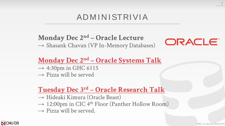
Monday Dec 2nd – Oracle Lecture→ Shasank Chavan (VP In-Memory Databases)

Monday Dec 2nd – Oracle Systems Talk→ 4:30pm in GHC 6115→ Pizza will be served

Tuesday Dec 3rd – Oracle Research Talk→ Hideaki Kimura (Oracle Beast)→ 12:00pm in CIC 4th Floor (Panther Hollow Room)→ Pizza will be served.

3

CMU 15-445/645 (Fall 2019)

L AST CL ASS

Atomic Commit Protocols

Replication

Consistency Issues (CAP)

Federated Databases

4

CMU 15-445/645 (Fall 2019)

BIFURCATED ENVIRONMENT

5

ExtractTransform

Load

OLAP DatabaseOLTP Databases

CMU 15-445/645 (Fall 2019)

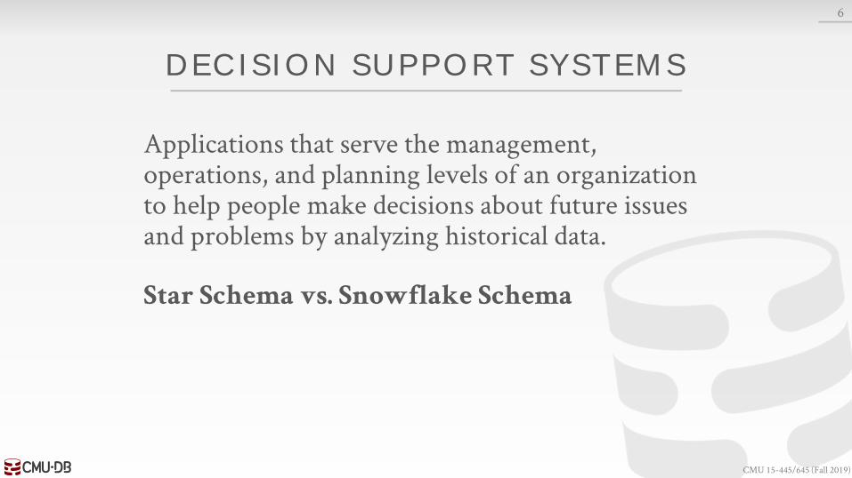
DECISION SUPPORT SYSTEMS

Applications that serve the management, operations, and planning levels of an organization to help people make decisions about future issues and problems by analyzing historical data.

Star Schema vs. Snowflake Schema

6

CMU 15-445/645 (Fall 2019)

STAR SCHEMA

7

CATEGORY_NAMECATEGORY_DESCPRODUCT_CODEPRODUCT_NAMEPRODUCT_DESC

PRODUCT_DIM

COUNTRYSTATE_CODESTATE_NAMEZIP_CODECITY

LOCATION_DIM

IDFIRST_NAMELAST_NAMEEMAILZIP_CODE

CUSTOMER_DIM

YEARDAY_OF_YEARMONTH_NUMMONTH_NAMEDAY_OF_MONTH

TIME_DIM

SALES_FACTPRODUCT_FKTIME_FKLOCATION_FKCUSTOMER_FK

PRICEQUANTITY

CMU 15-445/645 (Fall 2019)

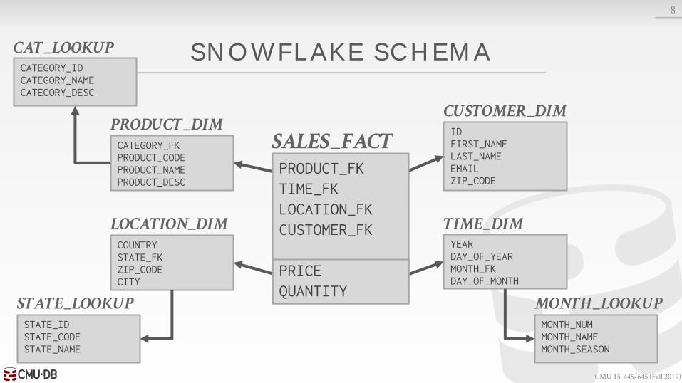
SNOWFL AKE SCHEMA

8

CATEGORY_FKPRODUCT_CODEPRODUCT_NAMEPRODUCT_DESC

PRODUCT_DIM

COUNTRYSTATE_FKZIP_CODECITY

LOCATION_DIM

IDFIRST_NAMELAST_NAMEEMAILZIP_CODE

CUSTOMER_DIM

YEARDAY_OF_YEARMONTH_FKDAY_OF_MONTH

TIME_DIM

SALES_FACTPRODUCT_FKTIME_FKLOCATION_FKCUSTOMER_FK

PRICEQUANTITY

CATEGORY_IDCATEGORY_NAMECATEGORY_DESC

CAT_LOOKUP

STATE_IDSTATE_CODESTATE_NAME

STATE_LOOKUPMONTH_NUMMONTH_NAMEMONTH_SEASON

MONTH_LOOKUP

CMU 15-445/645 (Fall 2019)

STAR VS. SNOWFL AKE SCHEMA

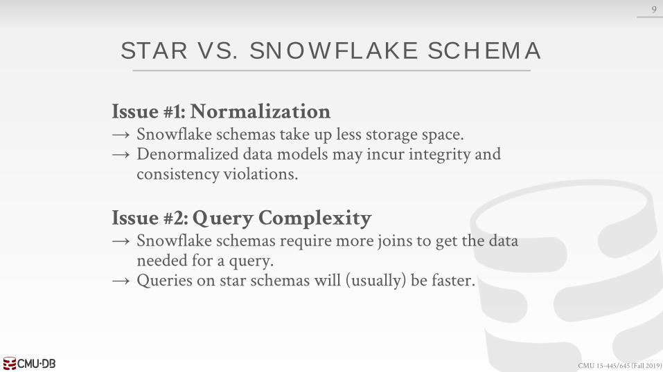
Issue #1: Normalization→ Snowflake schemas take up less storage space.→ Denormalized data models may incur integrity and

consistency violations.

Issue #2: Query Complexity→ Snowflake schemas require more joins to get the data

needed for a query.→ Queries on star schemas will (usually) be faster.

9

CMU 15-445/645 (Fall 2019)

P3 P4

P1 P2

PROBLEM SETUP

10

ApplicationServer

PartitionsSELECT * FROM R JOIN SON R.id = S.id

CMU 15-445/645 (Fall 2019)

P3 P4

P1 P2

PROBLEM SETUP

10

ApplicationServer

PartitionsSELECT * FROM R JOIN SON R.id = S.id

P2P4P3

CMU 15-445/645 (Fall 2019)

TODAY'S AGENDA

Execution Models

Query Planning

Distributed Join Algorithms

Cloud Systems

11

CMU 15-445/645 (Fall 2019)

PUSH VS. PULL

Approach #1: Push Query to Data→ Send the query (or a portion of it) to the node that

contains the data.→ Perform as much filtering and processing as possible

where data resides before transmitting over network.

Approach #2: Pull Data to Query→ Bring the data to the node that is executing a query that

needs it for processing.

12

CMU 15-445/645 (Fall 2019)

PUSH QUERY TO DATA

13

Node

ApplicationServer Node

P1→ID:1-100

P2→ID:101-200

SELECT * FROM R JOIN SON R.id = S.id

R ⨝ SIDs [101,200] Result: R ⨝ S

CMU 15-445/645 (Fall 2019)

Storage

PULL DATA TO QUERY

14

Node

ApplicationServer Node

Page ABC

Page XYZ

R ⨝ SIDs [101,200]

P1→ID:1-100

P2→ID:101-200

SELECT * FROM R JOIN SON R.id = S.id

CMU 15-445/645 (Fall 2019)

Storage

PULL DATA TO QUERY

14

Node

ApplicationServer Node

Page ABC

Page XYZ

R ⨝ SIDs [101,200]

P1→ID:1-100

P2→ID:101-200

SELECT * FROM R JOIN SON R.id = S.id

CMU 15-445/645 (Fall 2019)

Storage

PULL DATA TO QUERY

14

Node

ApplicationServer Node

R ⨝ SIDs [101,200]

P1→ID:1-100

P2→ID:101-200

SELECT * FROM R JOIN SON R.id = S.id

Result: R ⨝ S

CMU 15-445/645 (Fall 2019)

OBSERVATION

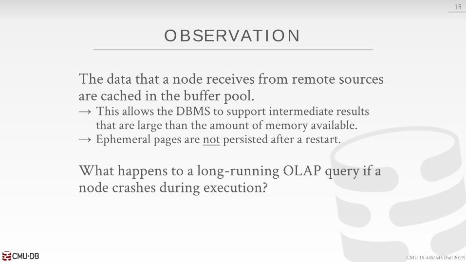
The data that a node receives from remote sources are cached in the buffer pool.→ This allows the DBMS to support intermediate results

that are large than the amount of memory available.→ Ephemeral pages are not persisted after a restart.

What happens to a long-running OLAP query if a node crashes during execution?

15

CMU 15-445/645 (Fall 2019)

QUERY FAULT TOLERANCE

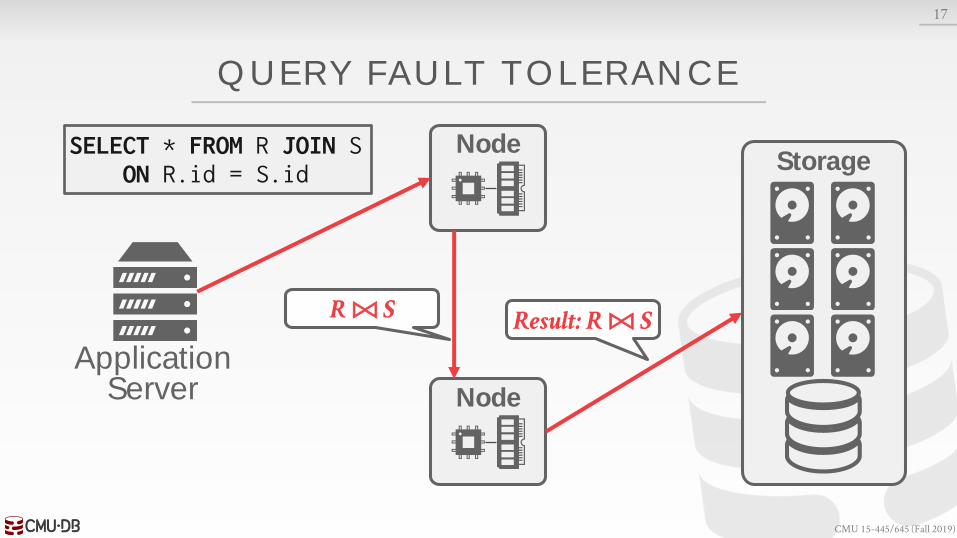
Most shared-nothing distributed OLAP DBMSs are designed to assume that nodes do not fail during query execution. → If one node fails during query execution, then the whole

query fails.

The DBMS could take a snapshot of the intermediate results for a query during execution to allow it to recover if nodes fail.

16

CMU 15-445/645 (Fall 2019)

Storage

QUERY FAULT TOLERANCE

17

Node

ApplicationServer Node

R ⨝ S

SELECT * FROM R JOIN SON R.id = S.id

Result: R ⨝ S

CMU 15-445/645 (Fall 2019)

Storage

QUERY FAULT TOLERANCE

17

Node

ApplicationServer Node

SELECT * FROM R JOIN SON R.id = S.id Result: R ⨝ S

CMU 15-445/645 (Fall 2019)

QUERY PL ANNING

All the optimizations that we talked about before are still applicable in a distributed environment.→ Predicate Pushdown→ Early Projections→ Optimal Join Orderings

Distributed query optimization is even harder because it must consider the location of data in the cluster and data movement costs.

18

CMU 15-445/645 (Fall 2019)

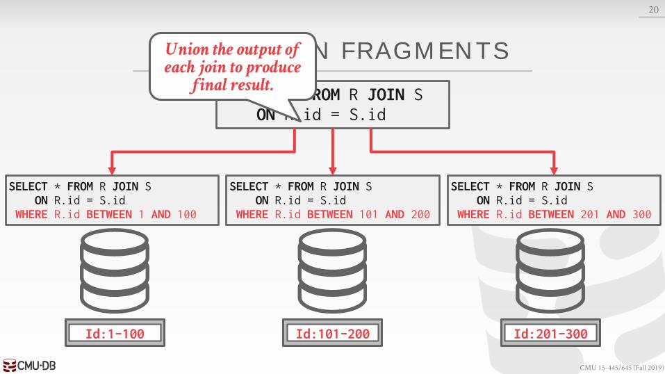
QUERY PL AN FRAGMENTS

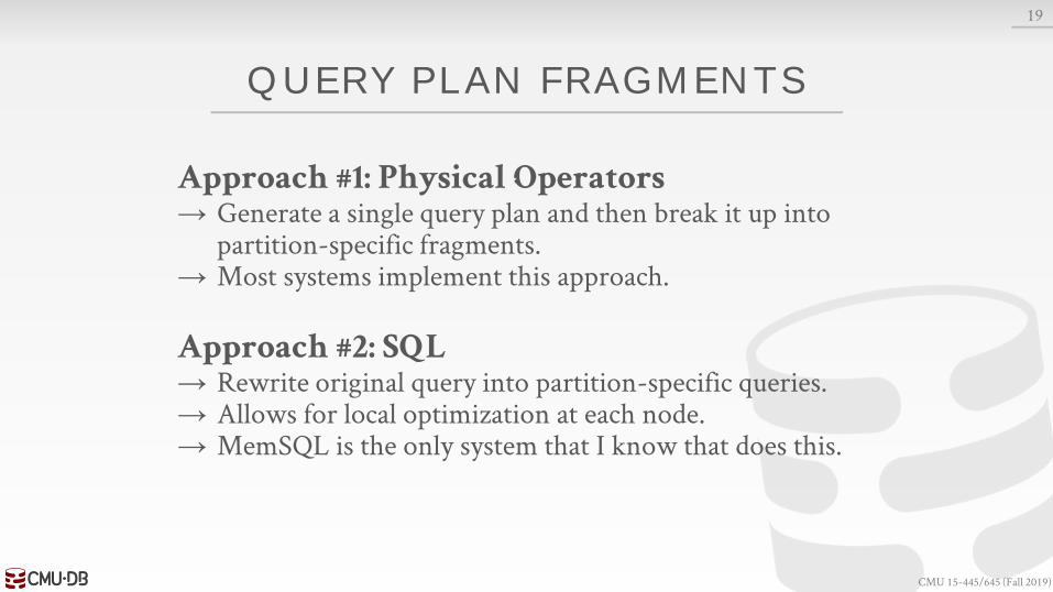
Approach #1: Physical Operators→ Generate a single query plan and then break it up into

partition-specific fragments.→ Most systems implement this approach.

Approach #2: SQL→ Rewrite original query into partition-specific queries.→ Allows for local optimization at each node.→ MemSQL is the only system that I know that does this.

19

CMU 15-445/645 (Fall 2019)

QUERY PL AN FRAGMENTS

20

SELECT * FROM R JOIN SON R.id = S.id

Id:1-100

SELECT * FROM R JOIN SON R.id = S.id

WHERE R.id BETWEEN 1 AND 100

Id:101-200

SELECT * FROM R JOIN SON R.id = S.id

WHERE R.id BETWEEN 101 AND 200

Id:201-300

SELECT * FROM R JOIN SON R.id = S.id

WHERE R.id BETWEEN 201 AND 300

CMU 15-445/645 (Fall 2019)

QUERY PL AN FRAGMENTS

20

SELECT * FROM R JOIN SON R.id = S.id

Id:1-100

SELECT * FROM R JOIN SON R.id = S.id

WHERE R.id BETWEEN 1 AND 100

Id:101-200

SELECT * FROM R JOIN SON R.id = S.id

WHERE R.id BETWEEN 101 AND 200

Id:201-300

SELECT * FROM R JOIN SON R.id = S.id

WHERE R.id BETWEEN 201 AND 300

Union the output of each join to produce

final result.

CMU 15-445/645 (Fall 2019)

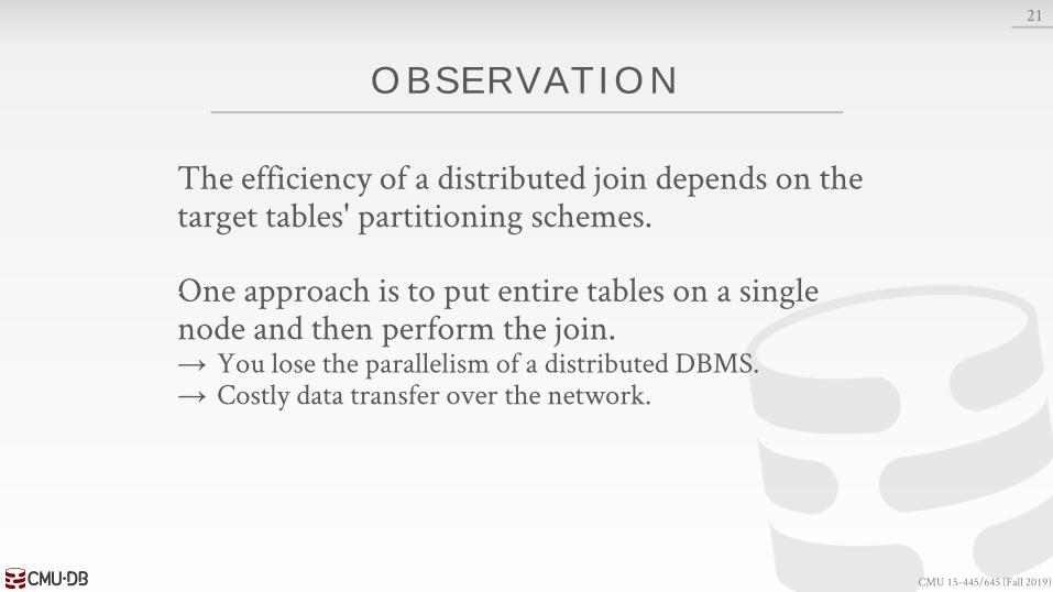
OBSERVATION

The efficiency of a distributed join depends on the target tables' partitioning schemes.

One approach is to put entire tables on a single node and then perform the join.→ You lose the parallelism of a distributed DBMS.→ Costly data transfer over the network.

21

CMU 15-445/645 (Fall 2019)

DISTRIBUTED JOIN ALGORITHMS

To join tables R and S, the DBMS needs to get the proper tuples on the same node.

Once there, it then executes the same join algorithms that we discussed earlier in the semester.

22

CMU 15-445/645 (Fall 2019)

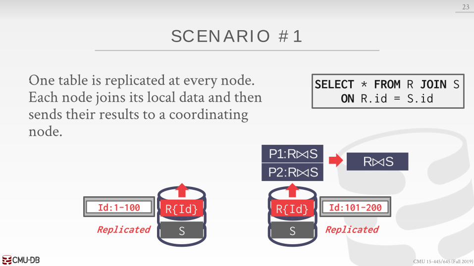
SCENARIO #1

One table is replicated at every node.Each node joins its local data and then sends their results to a coordinating node.

23

R{Id}

S

Id:1-100

Replicated

R{Id}

S

Id:101-200

Replicated

SELECT * FROM R JOIN SON R.id = S.id

P1:R⨝S P2:R⨝S

CMU 15-445/645 (Fall 2019)

SCENARIO #1

One table is replicated at every node.Each node joins its local data and then sends their results to a coordinating node.

23

R{Id}

S

Id:1-100

Replicated

R{Id}

S

Id:101-200

Replicated

SELECT * FROM R JOIN SON R.id = S.id

P1:R⨝S

P2:R⨝SR⨝S

CMU 15-445/645 (Fall 2019)

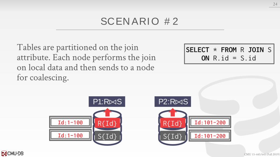
SCENARIO #2

Tables are partitioned on the join attribute. Each node performs the join on local data and then sends to a node for coalescing.

24

R{Id}

S{Id}

Id:1-100 R{Id}

S{Id}

Id:101-200

Id:1-100 Id:101-200

P1:R⨝S P2:R⨝S

SELECT * FROM R JOIN SON R.id = S.id

CMU 15-445/645 (Fall 2019)

SCENARIO #2

Tables are partitioned on the join attribute. Each node performs the join on local data and then sends to a node for coalescing.

24

R{Id}

S{Id}

Id:1-100 R{Id}

S{Id}

Id:101-200

Id:1-100 Id:101-200

P1:R⨝S

P2:R⨝SR⨝S

SELECT * FROM R JOIN SON R.id = S.id

CMU 15-445/645 (Fall 2019)

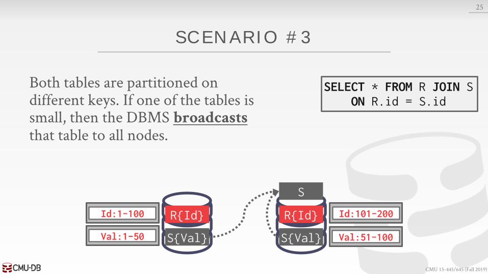
SCENARIO #3

Both tables are partitioned on different keys. If one of the tables is small, then the DBMS broadcaststhat table to all nodes.

25

R{Id}

S{Val}

Id:1-100 R{Id}

S{Val}

Id:101-200

Val:1-50 Val:51-100

SELECT * FROM R JOIN SON R.id = S.id

CMU 15-445/645 (Fall 2019)

SCENARIO #3

Both tables are partitioned on different keys. If one of the tables is small, then the DBMS broadcaststhat table to all nodes.

25

R{Id}

S{Val}

Id:1-100 R{Id}

S{Val}

Id:101-200

Val:1-50 Val:51-100

S

SELECT * FROM R JOIN SON R.id = S.id

CMU 15-445/645 (Fall 2019)

SCENARIO #3

Both tables are partitioned on different keys. If one of the tables is small, then the DBMS broadcaststhat table to all nodes.

25

R{Id}

S{Val}

Id:1-100 R{Id}

S{Val}

Id:101-200

Val:1-50 Val:51-100

S S

SELECT * FROM R JOIN SON R.id = S.id

CMU 15-445/645 (Fall 2019)

SCENARIO #3

Both tables are partitioned on different keys. If one of the tables is small, then the DBMS broadcaststhat table to all nodes.

25

R{Id}

S{Val}

Id:1-100 R{Id}

S{Val}

Id:101-200

Val:1-50 Val:51-100

S S

P1:R⨝S P2:R⨝S

SELECT * FROM R JOIN SON R.id = S.id

CMU 15-445/645 (Fall 2019)

SCENARIO #3

Both tables are partitioned on different keys. If one of the tables is small, then the DBMS broadcaststhat table to all nodes.

25

R{Id}

S{Val}

Id:1-100 R{Id}

S{Val}

Id:101-200

Val:1-50 Val:51-100

S S

P1:R⨝S

P2:R⨝SR⨝S

SELECT * FROM R JOIN SON R.id = S.id

CMU 15-445/645 (Fall 2019)

SCENARIO #4

Both tables are not partitioned on the join key. The DBMS copies the tables by reshuffling them across nodes.

26

R{Name}

S{Val}

Name:A-M R{Name}

S{Val}

Name:N-Z

Val:1-50 Val:51-100

SELECT * FROM R JOIN SON R.id = S.id

CMU 15-445/645 (Fall 2019)

SCENARIO #4

Both tables are not partitioned on the join key. The DBMS copies the tables by reshuffling them across nodes.

26

R{Name}

S{Val}

Name:A-M R{Name}

S{Val}

Name:N-Z

Val:1-50 Val:51-100

R{Id} Id:101-200

SELECT * FROM R JOIN SON R.id = S.id

CMU 15-445/645 (Fall 2019)

SCENARIO #4

Both tables are not partitioned on the join key. The DBMS copies the tables by reshuffling them across nodes.

26

R{Name}

S{Val}

Name:A-M R{Name}

S{Val}

Name:N-Z

Val:1-50 Val:51-100

R{Id}Id:1-100 R{Id} Id:101-200

SELECT * FROM R JOIN SON R.id = S.id

CMU 15-445/645 (Fall 2019)

SCENARIO #4

Both tables are not partitioned on the join key. The DBMS copies the tables by reshuffling them across nodes.

26

R{Name}

S{Val}

Name:A-M R{Name}

S{Val}

Name:N-Z

Val:1-50 Val:51-100

Id:101-200S{Id}

R{Id}Id:1-100 R{Id} Id:101-200

SELECT * FROM R JOIN SON R.id = S.id

CMU 15-445/645 (Fall 2019)

SCENARIO #4

Both tables are not partitioned on the join key. The DBMS copies the tables by reshuffling them across nodes.

26

R{Name}

S{Val}

Name:A-M R{Name}

S{Val}

Name:N-Z

Val:1-50 Val:51-100

Id:1-100 S{Id} Id:101-200S{Id}

R{Id}Id:1-100 R{Id} Id:101-200

SELECT * FROM R JOIN SON R.id = S.id

CMU 15-445/645 (Fall 2019)

SCENARIO #4

Both tables are not partitioned on the join key. The DBMS copies the tables by reshuffling them across nodes.

26

R{Name}

S{Val}

Name:A-M R{Name}

S{Val}

Name:N-Z

Val:1-50 Val:51-100

Id:1-100 S{Id} Id:101-200S{Id}

P1:R⨝S P2:R⨝S

R{Id}Id:1-100 R{Id} Id:101-200

SELECT * FROM R JOIN SON R.id = S.id

CMU 15-445/645 (Fall 2019)

SCENARIO #4

Both tables are not partitioned on the join key. The DBMS copies the tables by reshuffling them across nodes.

26

R{Name}

S{Val}

Name:A-M R{Name}

S{Val}

Name:N-Z

Val:1-50 Val:51-100

Id:1-100 S{Id} Id:101-200S{Id}

P1:R⨝S

P2:R⨝SR⨝S

R{Id}Id:1-100 R{Id} Id:101-200

SELECT * FROM R JOIN SON R.id = S.id

CMU 15-445/645 (Fall 2019)

SEMI-JOIN

Join operator where the result only contains columns from the left table.

Distributed DBMSs use semi-join to minimize the amount of data sent during joins.→ This is like a projection pushdown.

Some DBMSs support SEMI JOINSQL syntax. Otherwise you fake it with EXISTS.

27

SELECT R.id FROM RLEFT OUTER JOIN SON R.id = S.id

WHERE R.id IS NOT NULL

R S

S

CMU 15-445/645 (Fall 2019)

SEMI-JOIN

Join operator where the result only contains columns from the left table.

Distributed DBMSs use semi-join to minimize the amount of data sent during joins.→ This is like a projection pushdown.

Some DBMSs support SEMI JOINSQL syntax. Otherwise you fake it with EXISTS.

27

SELECT R.id FROM RLEFT OUTER JOIN SON R.id = S.id

WHERE R.id IS NOT NULL

R S

R

CMU 15-445/645 (Fall 2019)

SEMI-JOIN

Join operator where the result only contains columns from the left table.

Distributed DBMSs use semi-join to minimize the amount of data sent during joins.→ This is like a projection pushdown.

Some DBMSs support SEMI JOINSQL syntax. Otherwise you fake it with EXISTS.

27

SELECT R.id FROM RLEFT OUTER JOIN SON R.id = S.id

WHERE R.id IS NOT NULL

R S

SELECT R.id FROM RWHERE EXISTS (SELECT 1 FROM SWHERE R.id = S.id)

R.idR.id

CMU 15-445/645 (Fall 2019)

SEMI-JOIN

Join operator where the result only contains columns from the left table.

Distributed DBMSs use semi-join to minimize the amount of data sent during joins.→ This is like a projection pushdown.

Some DBMSs support SEMI JOINSQL syntax. Otherwise you fake it with EXISTS.

27

SELECT R.id FROM RLEFT OUTER JOIN SON R.id = S.id

WHERE R.id IS NOT NULL

R S

SELECT R.id FROM RWHERE EXISTS (SELECT 1 FROM SWHERE R.id = S.id)

R.id

R.id

CMU 15-445/645 (Fall 2019)

REL ATIONAL ALGEBRA: SEMI -JOIN

Like a natural join except that the attributes on the right table that are not used to compute the join are restricted.

Syntax: (R⋉ S)

28

a_id b_id xxx

a1 101 X1

a2 102 X2

a3 103 X3

R(a_id,b_id,xxx) S(a_id,b_id,yyy)a_id b_id yyy

a3 103 Y1

a4 104 Y2

a5 105 Y3

(R ⋉ S)a_id b_id xxx

a3 103 X3

CMU 15-445/645 (Fall 2019)

CLOUD SYSTEMS

Vendors provide database-as-a-service (DBaaS) offerings that are managed DBMS environments.

Newer systems are starting to blur the lines between shared-nothing and shared-disk.→ Example: You can do simple filtering on Amazon S3

before copying data to compute nodes.

29

CMU 15-445/645 (Fall 2019)

CLOUD SYSTEMS

Approach #1: Managed DBMSs→ No significant modification to the DBMS to be "aware"

that it is running in a cloud environment.→ Examples: Most vendors

Approach #2: Cloud-Native DBMS→ The system is designed explicitly to run in a cloud

environment. → Usually based on a shared-disk architecture.→ Examples: Snowflake, Google BigQuery, Amazon

Redshift, Microsoft SQL Azure

30

CMU 15-445/645 (Fall 2019)

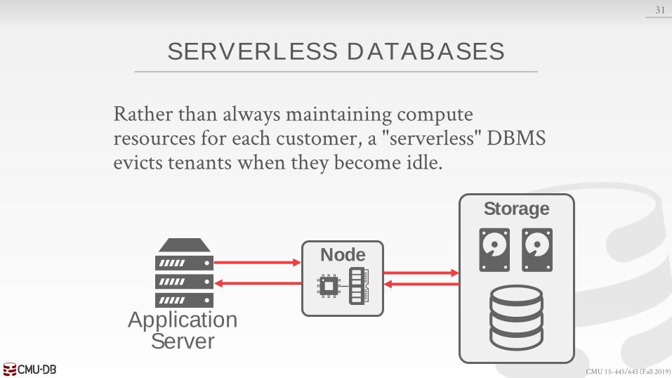
SERVERLESS DATABASES

Rather than always maintaining compute resources for each customer, a "serverless" DBMS evicts tenants when they become idle.

31

ApplicationServer

Node

CMU 15-445/645 (Fall 2019)

SERVERLESS DATABASES

Rather than always maintaining compute resources for each customer, a "serverless" DBMS evicts tenants when they become idle.

31

ApplicationServer

Node

CMU 15-445/645 (Fall 2019)

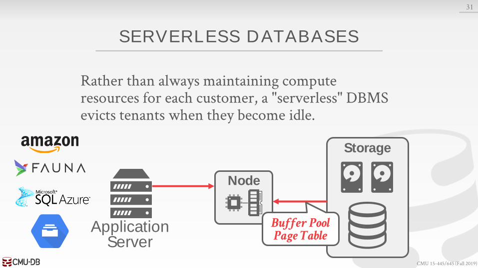
SERVERLESS DATABASES

Rather than always maintaining compute resources for each customer, a "serverless" DBMS evicts tenants when they become idle.

31

ApplicationServer

Node

Storage

CMU 15-445/645 (Fall 2019)

SERVERLESS DATABASES

Rather than always maintaining compute resources for each customer, a "serverless" DBMS evicts tenants when they become idle.

31

ApplicationServer

Node

StorageBuffer PoolPage Table

CMU 15-445/645 (Fall 2019)

SERVERLESS DATABASES

Rather than always maintaining compute resources for each customer, a "serverless" DBMS evicts tenants when they become idle.

31

ApplicationServer

Storage

CMU 15-445/645 (Fall 2019)

SERVERLESS DATABASES

Rather than always maintaining compute resources for each customer, a "serverless" DBMS evicts tenants when they become idle.

31

ApplicationServer

Node

Storage

Buffer PoolPage Table

CMU 15-445/645 (Fall 2019)

DISAGGREGATED COMPONENTS

System Catalogs→ HCatalog, Google Data Catalog, Amazon Glue Data

Catalog

Node Management→ Kubernetes, Apache YARN, Cloud Vendor Tools

Query Optimizers→ Greenplum Orca, Apache Calcite

32

CMU 15-445/645 (Fall 2019)

UNIVERSAL FORMATS

Most DBMSs use a proprietary on-disk binary file format for their databases.→ Think of the BusTub page types…

The only way to share data between systems is to convert data into a common text-based format→ Examples: CSV, JSON, XML

There are new open-source binary file formats that make it easier to access data across systems.

33

CMU 15-445/645 (Fall 2019)

UNIVERSAL FORMATS

Apache Parquet→ Compressed columnar storage from

Cloudera/Twitter

Apache ORC→ Compressed columnar storage from

Apache Hive.

Apache CarbonData→ Compressed columnar storage with

indexes from Huawei.

34

Apache Iceberg→ Flexible data format that supports

schema evolution from Netflix.

HDF5→ Multi-dimensional arrays for

scientific workloads.

Apache Arrow→ In-memory compressed columnar

storage from Pandas/Dremio.

CMU 15-445/645 (Fall 2019)

CONCLUSION

More money, more data, more problems…

Cloud OLAP Vendors:

On-Premise OLAP Systems:

35

CMU 15-445/645 (Fall 2019)

NEXT CL ASS

Oracle Guest Speaker

36