Embed Size (px)
Citation preview
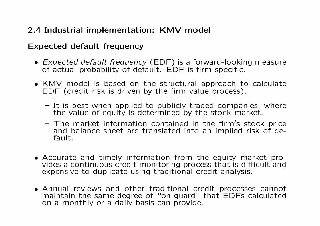
2.4 Industrial implementation: KMV model
Expected default frequency
• Expected default frequency (EDF) is a forward-looking measureof actual probability of default. EDF is firm specific.
• KMV model is based on the structural approach to calculateEDF (credit risk is driven by the firm value process).
– It is best when applied to publicly traded companies, wherethe value of equity is determined by the stock market.
– The market information contained in the firm′s stock priceand balance sheet are translated into an implied risk of de-fault.
• Accurate and timely information from the equity market pro-vides a continuous credit monitoring process that is difficult andexpensive to duplicate using traditional credit analysis.
• Annual reviews and other traditional credit processes cannotmaintain the same degree of “on guard” that EDFs calculatedon a monthly or a daily basis can provide.
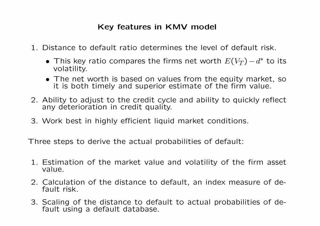
Key features in KMV model
1. Distance to default ratio determines the level of default risk.
• This key ratio compares the firms net worth E(VT )−d∗ to itsvolatility.
• The net worth is based on values from the equity market, soit is both timely and superior estimate of the firm value.
2. Ability to adjust to the credit cycle and ability to quickly reflectany deterioration in credit quality.
3. Work best in highly efficient liquid market conditions.
Three steps to derive the actual probabilities of default:
1. Estimation of the market value and volatility of the firm assetvalue.
2. Calculation of the distance to default, an index measure of de-fault risk.
3. Scaling of the distance to default to actual probabilities of de-fault using a default database.

• Changes in EDF tend to anticipate at least one year earlier thanthe downgrading of the issuer by rating agencies like Moodysand S & Ps
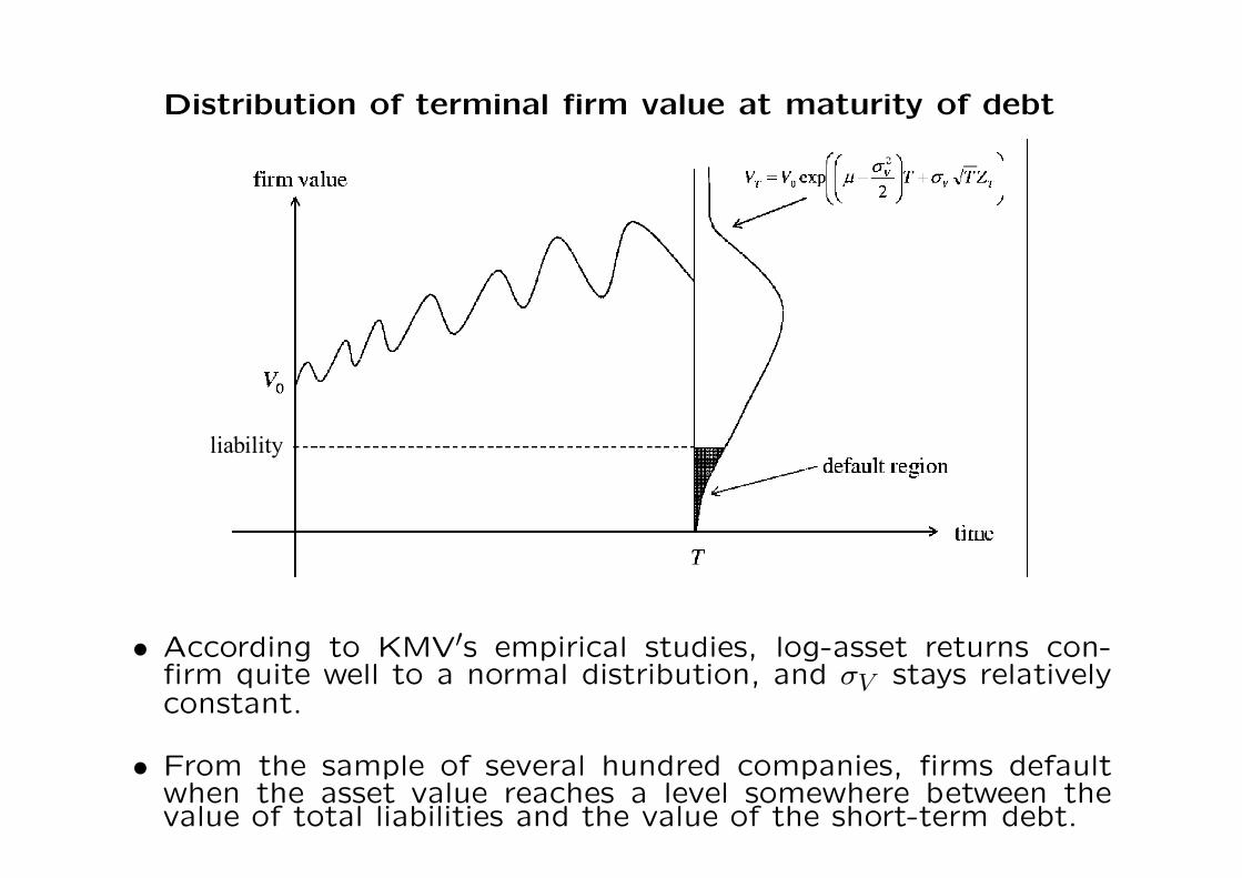
Distribution of terminal firm value at maturity of debt
• According to KMV′s empirical studies, log-asset returns con-firm quite well to a normal distribution, and σV stays relativelyconstant.
• From the sample of several hundred companies, firms defaultwhen the asset value reaches a level somewhere between thevalue of total liabilities and the value of the short-term debt.

Distance to default
Default point, d∗ = short-term debt +1
2× long-term debt. Why
1
2?
Why not!
From VT = V0 exp
((µ −
σ2
2
)T + σV ZT
), the probability of finishing
below D at date T is
N
−
ln V0D +
(µ − σ2
2
)T
σV
√T
.
Distance to default is defined by
df =E(VT ) − d∗
σ̂V
√T
=ln V0
d∗ +(µ − σ̂2
V2
)T
σ̂V
√T
,
where V0 is the current market value of firm, µ is the expected rateof return on firm value and σ̂V is the annualized firm value volatility.The probability of default is a function of the firm’s capital structure,the volatility of the asset returns and the current asset value.
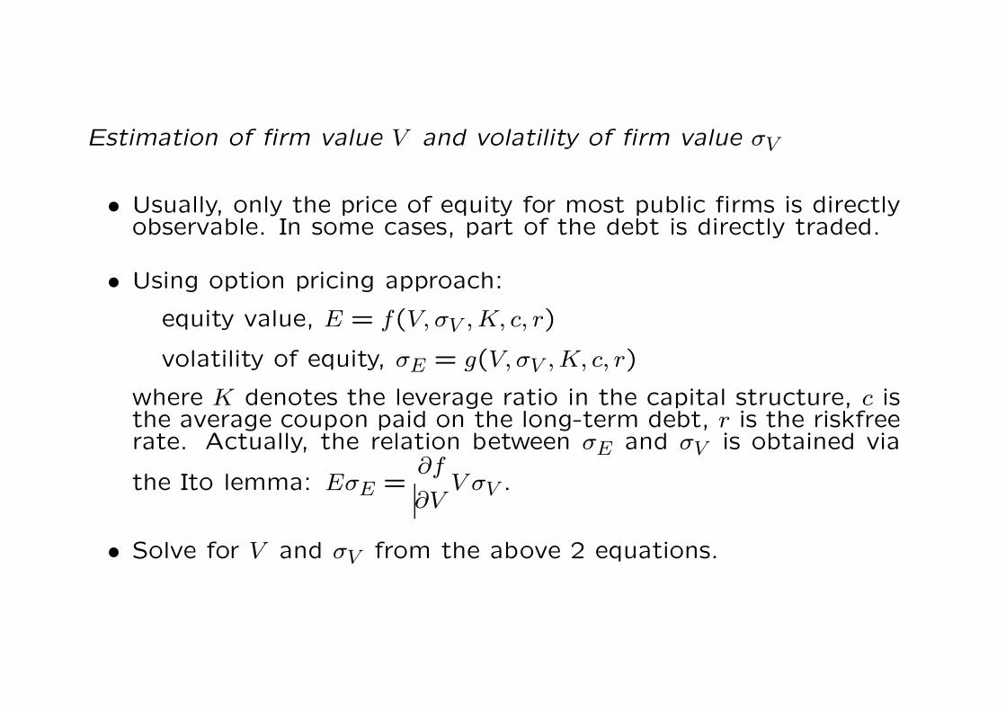
Estimation of firm value V and volatility of firm value σV
• Usually, only the price of equity for most public firms is directlyobservable. In some cases, part of the debt is directly traded.
• Using option pricing approach:
equity value, E = f(V, σV , K, c, r)
volatility of equity, σE = g(V, σV , K, c, r)
where K denotes the leverage ratio in the capital structure, c isthe average coupon paid on the long-term debt, r is the riskfreerate. Actually, the relation between σE and σV is obtained via
the Ito lemma: EσE =∂f
∂VV σV .
• Solve for V and σV from the above 2 equations.

Probabilities of default from the default distance
Based on historical information on a large sample of firms, for eachtime horizon, one can estimate the proportion of firms of a givendefault distance (say, df = 4.0) which actually defaulted after oneyear.

Example Federal Express (dollars in billion of US$)
November 1997 February 1998Market capitalization $7.9 $7.3(price × shares outstanding)Book liabilities $4.7 $4.9Market value of assets $12.6 $12.2Asset volatility 15% 17%Default point $3.4 $3.5
Default distance12.6 − 3.4
0.15
12.2 − 3.5
0.17EDF 0.06%(6bp) = AA− 0.11%(11bp) = A−
The causes of changes for an EDF are due to variations in the stockprice, debt level (leverage ratio), and asset volatility .
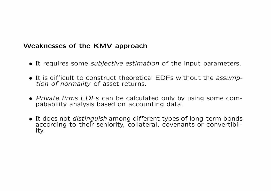
Weaknesses of the KMV approach
• It requires some subjective estimation of the input parameters.
• It is difficult to construct theoretical EDFs without the assump-tion of normality of asset returns.
• Private firms EDFs can be calculated only by using some com-pabability analysis based on accounting data.
• It does not distinguish among different types of long-term bondsaccording to their seniority, collateral, covenants or convertibil-ity.

Conversion of actual EDF into risk neutral EDF
When we price credit derivatives, we need to have the informationon the risk neutral probabilities of default. Under Q
dV ∗t
V ∗t
= r dt + σ dZt.
Let Q̂T = Pr[V∗T ≤ DPTT ]
= probability that the asset value at Tfalls below DPTT under Q
= N(−d∗2)where
d∗2 =ln V0
DPTT+(r − σ2
2
)T
σ√
T.
On the other hand, EDFT = N(−d2) where d2 =ln V0
DPTT+(µ − σ2
2
)T
σ√
T.
Now, −d2 +(µ − r)
√T
σ= −d∗2 so that
Q̂T = N
[N−1(EDFT ) +
µ − r
σ
√T
].

Since µ ≥ r, we have Q̂T ≥ EDFT .
According to CAPM , µ − r = βπ
where β = beta of the asset with the market
= ρσ
σM=
cov(R, RM)
var(RM),
Here, R and RM are the return of firm asset and market portfolio,
ρ = correlation coefficient between the asset returns and
market’s return
π = market risk premium for one unit of beta risk = µM −r.
Finally,µ − r
σ=
βπ
σ= ρ
π
σM= ρU , where U =
µM − r
σMis the market
Sharpe ratio. The market Sharpe ratio is the excess return per unitof market volatility for the market portfolio.
![ПЕРСОНА ДДМИТРИЙМИТРИЙ ДЕГТЯРЕВ KMV 103 web.pdf · [1] сентябрь 2017 СТАБИЛЬНОСТЬ ПЕРСОНА ДЕГТЯРЕВ ДДМИТРИЙМИТРИЙ](https://img.pdfslide.net/doc/110x75/6050042051bf88652a4e7f48/-oeoe-kmv-103-webpdf-1.jpg)