Embed Size (px)
Citation preview
2D Compressible Viscous-Flow Solver on
Unstructured Meshes with Linear and
Quadratic Reconstruction of Convective
Fluxes
Interim Project Report
Master of Technology
By
Mohamed Yousuf .A .U
( Roll No. 04410304 )
DEPARTMENT OF MECHANICAL ENGINEERING
INDIAN INSTITUTE OF TECHNOLOGY GUWAHATI
NOVEMBER-2005
CERTIFICATE
This is to certify that the work contained in this thesis entitled “Computation
of Compressible, inviscid and viscous turbomachinary cascade flows
on structured and unstructured meshes ” by Mohamed Yousuf .A.U
(04410304), has been carried out in the Department of Mechanical Engineering,
Indian Institute of Technology Guwahati under my supervision and that it has not
been submitted elsewhere for a degree.
Dr. Anoop. K. Dass
Associate Professor,
July, 2005 Dept. of Mechanical Engineering ,
Guwahati. Indian Institute of Technology Guwahati, Assam.

ACKNOWLEDGEMENT
I feel honored to express my deepest and most sincere gratitude to my thesis su-
pervisor, Dr. Anoop. K. Dass, for his invaluable guidance, kind suggestion and
encouragement throughout the progress of this work. I am highly indebted to him
for providing me ample freedom to work my way and simultaneously giving me a
taste of research work.
I would also like to take this opportunity to express my sense of gratitude to the
other faculty members for their kind help and encouragement and to all the non-
teaching staff of the department, without whose help, I would not have completed
this project work.
I heartily thank my senior Gundeti Lavan kumar and Suresh Kumar for his kind
suggestions and encouragement. I wish to record the help extended to me by all my
friends especially to Khaja Nijamudeen, Prabodh, Tapan Mishra, Sajeed, Sunil and
Vishnuvardhana Rao for their helpful discussions and encouragement. Also I would
like to thank my dear friends and all my classmates for their good company during
my stay at IIT Guwahati. I would also like to thank all the members of my family
for their tremendous support and love all through.
3

November 13, 2005
Contents
List of Figures iii
Nomenclature vi
1 Introduction 4
1.1 Motivation and Aim . . . . . . . . . . . . . . . . . . . . . . . . . . . 4
1.2 Literature Review . . . . . . . . . . . . . . . . . . . . . . . . . . . . . 5
1.3 Organization of Report . . . . . . . . . . . . . . . . . . . . . . . . . . 7
2 Governing Equations and Upwind Schemes 8
2.1 2D Navier-Stokes equations . . . . . . . . . . . . . . . . . . . . . . . 8
2.2 Upwind schemes . . . . . . . . . . . . . . . . . . . . . . . . . . . . . . 10
2.3 Basic principles of upwind discretization . . . . . . . . . . . . . . . . 12
2.4 Flux-vector splitting schemes . . . . . . . . . . . . . . . . . . . . . . 13
2.4.1 van Leer’s flux-vector splitting (FVS) . . . . . . . . . . . . . . 14
2.4.2 Roe’s flux-difference splitting (FDS) . . . . . . . . . . . . . . . 15
i
2.4.3 AUSM+ . . . . . . . . . . . . . . . . . . . . . . . . . . . . . . 17
3 Finite Volume Method 20
3.1 Introduction . . . . . . . . . . . . . . . . . . . . . . . . . . . . . . . . 20
3.2 The conservative discretization . . . . . . . . . . . . . . . . . . . . . . 21
3.3 Finite volume method . . . . . . . . . . . . . . . . . . . . . . . . . . 22
3.4 Different frameworks in FVM . . . . . . . . . . . . . . . . . . . . . . 23
3.4.1 Cell-centered versus cell vertex schemes . . . . . . . . . . . . . 24
3.5 Discretization of N-S equations . . . . . . . . . . . . . . . . . . . . . 25
3.5.1 Discretization of viscous fluxes . . . . . . . . . . . . . . . . . . 27
3.6 Reconstruction and limiting . . . . . . . . . . . . . . . . . . . . . . . 28
3.6.1 Multi-dimensional linear reconstruction of cell averaged data . 29
3.7 Quadratic-reconstruction . . . . . . . . . . . . . . . . . . . . . . . . . 34
3.8 Limiters . . . . . . . . . . . . . . . . . . . . . . . . . . . . . . . . . . 37
3.9 Jawahar and Kamath limiter . . . . . . . . . . . . . . . . . . . . . . . 41
3.10 Multistage time stepping . . . . . . . . . . . . . . . . . . . . . . . . . 41
3.11 Boundary conditions . . . . . . . . . . . . . . . . . . . . . . . . . . . 42
3.11.1 Inviscid or slip wall boundary condition . . . . . . . . . . . . . 43
3.11.2 Viscous or no-slip boundary condition . . . . . . . . . . . . . 45
3.11.3 Farfield boundary condition . . . . . . . . . . . . . . . . . . . 45
ii
3.11.4 Inflow/Outflow boundary conditions . . . . . . . . . . . . . . 46
4 Code Validation 48
4.1 NACA 0012 airfoil . . . . . . . . . . . . . . . . . . . . . . . . . . . . 49
4.2 Transonic flow over a bump in a channel . . . . . . . . . . . . . . . . 55
4.3 Flow past a staggered-biplane configuration . . . . . . . . . . . . . . 58
4.4 Viscous flow past a staggered-biplane configuration . . . . . . . . . . 61
5 Conclusions and Future Work 63
5.1 Scope for future work . . . . . . . . . . . . . . . . . . . . . . . . . . . 63
iii
List of Figures
3.1 Conservation laws for subvolumes of volume Ω . . . . . . . . . . . . . 21
3.2 (a) Cell centered , (b) Cell vertex (median dual) finite volume methods 24
3.3 2D finite volume method . . . . . . . . . . . . . . . . . . . . . . . . 26
3.4 Gradient computation at faces . . . . . . . . . . . . . . . . . . . . . 27
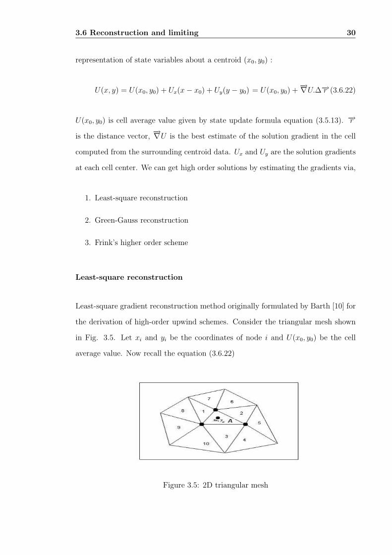
3.5 2D triangular mesh . . . . . . . . . . . . . . . . . . . . . . . . . . . . 30
3.6 Frink’s reconstruction . . . . . . . . . . . . . . . . . . . . . . . . . . . 33
3.7 The identification of more neighbors and flux integration path showed
by dashed line . . . . . . . . . . . . . . . . . . . . . . . . . . . . . . . 35
3.8 Mirror boundary condition . . . . . . . . . . . . . . . . . . . . . . . . 45
4.1 NACA 0012 airfoil grid pattern . . . . . . . . . . . . . . . . . . . . . 49
4.2 Pressure contours of flow over NACA 0012 airfoil problem (M∞ =
0.80, α = 1.25o) . . . . . . . . . . . . . . . . . . . . . . . . . . . . . . 50
4.3 Cp comparison of various schemes with no-limiter (Flow over NACA
0012 airfoil with M∞ = 0.80, α = 1.25o) . . . . . . . . . . . . . . . . 51
iv
4.4 Cp comparison of high order schemes with limiter (Flow over NACA
0012 airfoil with M∞ = 0.80, α = 1.25o) . . . . . . . . . . . . . . . . . 52
4.5 Comparison of high order schemes for flow over NACA 0012 airfoil
with M∞ = 0.80, α = 1.25o . . . . . . . . . . . . . . . . . . . . . . . . 53
4.6 Comparison high order schemes for flow over NACA 0012 airfoil prob-
lem with M∞ = 1.20, α = 0o . . . . . . . . . . . . . . . . . . . . . . . 54
4.7 Bump in a channel mesh pattern . . . . . . . . . . . . . . . . . . . . 55
4.8 Transonic channel flow M∞ = 0.85, t/c =4.2% . . . . . . . . . . . . . 56
4.9 Comparison of pressure distributions along the lower wall for tran-
sonic bump in a channel flow M∞ = 0.85, t/c = 4.2% . . . . . . . . . 57
4.10 Second order residual history . . . . . . . . . . . . . . . . . . . . . . 57
4.11 NACA 0012 biplane mesh . . . . . . . . . . . . . . . . . . . . . . . . 58
4.12 Pressure contours . . . . . . . . . . . . . . . . . . . . . . . . . . . . . 58
4.13 Adaptively generated mesh results M = 0.7, α = 0.00 . . . . . . . . 60
4.14 Viscous flow past staggered biplane airfoil 2nd order results M∞ =
0.8, α = 10o, Re∞ = 500 . . . . . . . . . . . . . . . . . . . . . . . . . 62
v
Nomenclaturec Speed of sound
Cd Coefficient of drag
Cl Coefficient of lift
Cp Coefficient of pressure
dS Surface formed by the boundary of the con-
trol volume
d(c) Degree of a cell (number of faces bounding
the face)
e Specific energy
F, G Vector of conservative fluxes in the x and y
directions
H Total enthalpy
M Mach number
nx, ny Direction cosines of the unit outward normal
to the interface
p Pressure
Q Source term
R1, R2, R3 Riemann invariants
~S Surface vector
t Time
U Vector of conserved variables
u, v Cartesian components of the velocity vector
V Velocity vector
x, y Cartesian components
4t Time step
4x,4y Spatial mesh step in x, y directions
−→∇U Gradient vector of the conserved variables
−→∇r Distance vector
vi
1
Greek Letters
Ω Control volume
ρ Density
γ Specific heat ratio
α Angle of attack
Subscript
c Centroid of cell
f Fictitious state
I Interior state
L,R Left and right states
‖ Component parallel to the interface of the
control volume side
x Component in x directioin
⊥ Component perpendicular to the control vol-
ume side
Superscript
+ Positive
− Negative
t Time step
AGARD: Advisory Group for Aerospace Research and Development
GAMM: German Association for Applied Mathematics and Mechanics
NACA: National Advisory Committee for Aeronautics (NASA)
NASA: National Aeronautics and Space Administration
NACA 0012: 12 thick symmetrical airfoil
VKI: Von Karman Institute

2
Abstract
This work is mainly concerned with the enhancement of the finite volume code for
computation of compressible viscous and inviscid flows. As the code is intended to
be somewhat general in nature and it is based on unstructured grid data structure.
The code can be used for or adapted to any new geometry just by making minor
changes in preprocessor (and without touching the solver). The inviscid part of the
code is validated by extensive comparison with single NACA 0012 airfoil flow, bump
in a channel flow and staggered biplane flow results. The viscous part is validated
by solving a staggered biplane airfoil problem. The accuracy of the solver is uplifted
by quadratic reconstruction.
Chapter 1
Introduction
1.1 Motivation and Aim
The history of Computational Fluid Dynamics started in the early 1970’s. Around
that time, it became an acronym for a combination of physics, numerical mathemat-
ics, and, to some extent, computer sciences employed to simulate fluid flows. The
beginning of CFD was triggered by the availability of increasingly more powerful
mainframes and the advances in CFD are still tightly coupled to the evolution of
computer technology. Among the first applications of the CFD methods was the
simulation of transonic flows based on the solution of non-linear potential equation.
Thanks to the rapidly increasing speed of supercomputers and due to the develop-
ment of a variety of numerical schemes and acceleration techniques, it was possible
to compute inviscid flows past complete aircraft configurations or inside of turbo-
machines. With the mid 1980’s, the focus started to shift to the significantly more
demanding simulation of viscous flows governed by the Navier-Stokes equations.
Due to the steadily increasing demands on the complexity and fidelity of flow simu-
lations, grid generation methods had to become more and more sophisticated. The
1.2 Literature Review 5
development started first with relatively simple structured meshes constructed either
by algebraic methods or by using partial differential equations. But with increas-
ing geometrical complexity of the configurations, the grid had to be broken into a
number of topologically simpler blocks. However, the generation of a structured,
multiblock grid for a complicated geometry may still take weeks to accomplish.
Therefore, the research also focused on the development of unstructured grid gener-
ators (and flow solvers), which promise significantly reduced setup times, with only
a minor user intervention. Nowadays, CFD methodologies are routinely employed
in the fields of aircraft, turbomachinery, car and ship design. Furthermore, CFD is
also applied in meteorology, oceanography, astrophysics, in oil recovery, and also in
architecture.
The present work aims to analyze the compressible flow field for transonic and
supersonic cases. A cell-centered finite volume method is used to solve 2D Euler
and Navier-Stokes equations on unstructured meshes. The solution accuracy of
solver is improved by implementing quadratic reconstruction.
1.2 Literature Review
The concept of using arbitrary control volumes to solve numerically the conserva-
tion laws was established in the late 70’s. Jameson and Mavriplis [1] reported some
of the earliest results from solving the 2D Euler equations on regular triangular
grids that were obtained by subdividing the quadrilateral grids. Their work is an
extension of what was established for finite volume schemes on structured grids to
triangular mesh, in a cell-centered framework. Godunov [2] introduced a high level
physics in the discretization procedure by solving the Riemann problem at cell inter-
faces. The solution is considered constant in each control volume and equal to the
cell-averages. The resolution of such Riemann problems remains however complex
1.2 Literature Review 6
and time consuming. Moreover, the averaging procedure at each time step causes
loss of many information. Therefore the problem is usually not solved exactly. On
the contrary, approximate forms are considered. Roe scheme [3] is one of the most
popular approximate Riemann’s solvers. This is based on characteristic decomposi-
tion of flux difference while ensuring the conservation property of the scheme. This
scheme has shown to be very accurate and particularly suited for explicit upwind
formulation. However, it suffers from carbuncle phenomenon at high Mach numbers.
Making use of similarity transformations and homogeneity property of Euler equa-
tions, Steger and Warming [4] split the flux depending on the sign of eigen values of
the flux Jacobian matrix. This splitting method produces errors at sonic point and
stagnation point due to discontinuity in flux Jacobian at these points. van Leer [5]
proposed an alternative splitting, which gives noticeably better results and resolves
steady shock profiles in at most two zones. For solving contact discontinuities and
shear layers the FVS schemes, however, exhibited a serious disadvantage by having
excessive numerical dissipation leading to significant errors in viscous calculations
In another effort to develop less dissipative upwind schemes, introducing the fla-
vor of the FDS scheme into FVS scheme reduces the surplus dissipation of the FVS.
In the 90’s, the new schemes are introduced to overcome the difficulties in earlier
methods. One is the AUSM (Advection Upstream Splitting Method) proposed by
Liou and Steffen [6] in 1993. This scheme is robust and converges as fast as the Roe
splitting. Even though the scheme, AUSM, enjoys remarkable success, post shock
overshoot and a glitch in the slowly moving shock are the drawbacks in AUSM
scheme. As a result, a new version, termed AUSM+, has been derived and is shown
in Liou paper [7].
Jameson [8] brought significant development in time marching methods using Runge-
1.3 Organization of Report 7
Kutta time marching technique. He demonstrated that the convergence of a time
dependent hyperbolic system to a steady state can be substantially accelerated by
the introduction of multiple grids. Barth and Jesperson [9] introduced a novel up-
wind scheme for the solution of Euler equations on unstructured meshes. This
scheme first performs a linear reconstruction to interpolate data to the control vol-
ume faces and then employs an approximate Riemann solver to compute the fluxes.
Limiting function is introduced to preserve monotonicity.
Based on the work of Barth and Fredrickson [10], Barth developed the concept
of K- exact reconstruction scheme [11], i.e., a reconstruction exact for a polynomial
of degree k. The polynomial in Barth’s method is defined in a way which guarantees
the conservation of the mean. Delanaye and Essers [12] developed a particular form
of quadratic reconstruction for the cell-centered scheme which is computationally
more efficient than the method of Barth.
1.3 Organization of Report
The report has been organized in 5 chapters and the outline is as follows: Chapter
2 presents the governing equations and upwind schemes. Chapter 3 gives an idea
about finite volume technique and its formulations for solution of 2-D Navier-Stokes
equations. Besides that the boundary conditions are also discussed in this chapter.
In chapter 4 the inviscid and viscous part of the code are validated. Chapter 5
mentions about conclusions and future flow path of the project.
Chapter 2
Governing Equations and Upwind
Schemes
2.1 2D Navier-Stokes equations
Conservation form of 2D compressible, Navier-Stokes equations can be written in
form of a vector of conservative variables ~U and two flux vectors ~F and ~G. ~FI and
~GI are the vectors of convective or inviscid terms and ~FV and ~GV are the vectors
of viscous terms. In absence of source terms nondimensional form of compressible
Navier-Stokes equations can be written as
∂U
∂t+
∂(FI − FV )
∂x+
∂(GI −GV )
∂y= 0 (2.1.1)
U =
ρ
ρu
ρv
e
FI =
ρu
ρu2 + p
ρuv
(e + p)u
GI =
ρv
ρvu
ρv2 + p
(e + p)v
(2.1.2)
2.1 2D Navier-Stokes equations 9
FV =1
ReL
0
τxx
τxy
uτxx + vτxy+ − qx
GV =1
ReL
0
τxy
τyy
uτxy + vτyy − qy
(2.1.3)
τxx = 2µ∂u
∂x−µ
2
3
(∂u
∂x+
∂v
∂y
)τyy = 2µ
∂v
∂y−2
3µ
(∂u
∂x+
∂v
∂y
)τxy = µ
(∂u
∂y+
∂v
∂x
)(2.1.4)
qx = − µ
(γ − 1)M2∞Pr
∂T
∂xqy = − µ
(γ − 1)M2∞Pr
∂T
∂y(2.1.5)
The nondimensionalization carried out using freestream variables ρ∞, U∞ and T∞.
M∞ is U∞/c∞. Reynolds number defined based on characteristic length ReL =
ρ∞U∞L/µ∞. Prandtl number is taken as 0.72. For mathematical closure of the
equations we use the equation of state
p = ρRT (2.1.6)
e is the sum of internal energy and kinetic energy given as
e = ρCvT +1
2ρ(u2 + v2) (2.1.7)
µ is nondimensionalized using Sutherland’s law
µ
µ∞=
(T
T∞
) 32 T∞ + S1
T + S1(2.1.8)
S1 is the Sutherland’s constant 110. If viscous terms are set to zero, then the
equation is transformed to a 2D unsteady compressible inviscid flow equations.
2.2 Upwind schemes 10
2.2 Upwind schemes
The system of compressible Navier-Stokes equations are second order partial differ-
ential equations. These equations are parabolic-hyperbolic in time and space but a
mixed elliptic-hyperbolic nature in space for stationary formulation. As described
in section 2.1, the Navier-Stokes equations can be split into convective and viscous
terms. The unsteady compressible inviscid flow equations are hyperbolic in nature
and viscous terms are elliptic in nature. We need special attention for the inviscid
equations. The property of nonlinear hyperbolic system of equations allow disconti-
nuities in the solution even if the initial data is smooth. Numerical methods which
need the mathematical continuity assumption may not predict these discontinuities
present in the solution accurately. Hence when defining numerical methods for such
equations physical propagation of perturbations, along characteristics should be con-
sidered. The schemes which consider physical properties of the flow equations are
popularly known as upwind schemes. Central schemes require lower numerical effort
or less CPU time for evaluation. But these schemes do not consider the character-
istic wave information direction and hence poor accuracy at discontinuities.
Upwind differencing represents an attempt to include our knowledge of the charac-
ter of the equations in our difference expressions. The basic idea behind upwinding
was first proposed in a landmark paper by Courant, Isaacson and Rees [15]. Their
paper dealt with the one-dimensional linear advection equation and proposed taking
one-sided differences based on the sign of the wave speed. In an upwind formulation,
there are two states on either side of a face which must be resolved into a single
value for the flux through the face.
Upwind schemes roughly divided into four main groups.
1. Flux vector splitting
2. Flux difference splitting
3. Total variation diminishing (TVD)
2.2 Upwind schemes 11
4. Fluctuation splitting
1. Flux vector splitting
One class of flux vector splitting (FVS) scheme decomposes the vector of the con-
vective fluxes in to two parts according to the sign of certain characteristic variables,
which are in general similar to but not identical with eigenvalues of the convective
flux Jacobian. The two parts of the flux vector are then discretized by upwind bi-
ased differences. The very first FVS schemes of this type developed in the beginning
by Steger and Warming and van Leer, respectively. Second class of FVS schemes
decompose the flux vector into a convective and a pressure (an acoustic) part. This
idea is utilized by schemes like AUSM (Advection Upstream Splitting Method) of
Liou et al [6], or CUSP scheme (Convective Upwind Split Pressure) of Jameson [16]
respectively. The second group of FVS schemes gained recently larger popularity
particularly because of their improved resolution of shear layers with only moderate
computational effort. An advantage of FVS schemes is also that they can easily
extended to real gas flows, as opposed to flux difference splitting or TVD schemes.
2. Flux difference splitting
Flux difference splitting schemes evaluate the convective fluxes at a face of control
volume from the left and right state by solving Riemann (shock tube) problem. The
idea to solve Riemann problem was first introduced by Godunov [2]. In order to
reduce numerical effort required for exact solution of Riemann problem, approximate
Riemann solvers was developed, e.g., Roe [3] and Osher et al [17].
3. TVD Schemes
The idea of TVD schemes first introduced by Harten in 1983. The TVD schemes
based on concept aimed at preventing the generation of new extrema in flow solution.
The principal condition for a TVD scheme are that maxima must be non increasing,
2.3 Basic principles of upwind discretization 12
minima non decreasing and no new local extrema may be created. Such scheme is
called monotonicity preserving. This property allows to resolve a shock wave with-
out any spurious oscillations of solutions. The disadvantage of TVD scheme is that
they can not easily extended to higher than second order accuracy. This limitation
can be overcome using ENO (Essentially Non-Oscillatory) discretization scheme.
4. Fluctuation splitting
Fluctuation splitting provides true multi dimensional upwinding. All upwind schemes
split the equation according to orientation of grid cells. But fluctuation splitting
schemes aims at resolve flow features which are not aligned with the grid. The flow
variables are associated with the grid nodes. Intermediate residuals are computed
as flux balances over the grid cells, which consists of triangles in 2D and tetrahedra
in 3D. The cell based residuals are then distributed in an upwind biased manner to
all the nodes. After that the solution is updated using nodal values. So far these
schemes are used only in research codes. This can be attributed to the complexity
and high numerical effort, as well as to convergence problems.
2.3 Basic principles of upwind discretization
The one dimensional wave equation is given by
∂U
∂t+ c
∂U
∂x= 0 (2.3.9)
Courant discretized the wave equation based on the sign of eigenvalue c. for c > 0
Uin+1 − Ui
n
4t+ c
Uin − Ui−1
n
4x= 0 (2.3.10)
2.4 Flux-vector splitting schemes 13
or
Uin+1 = Ui − λ(Ui
n − Ui−1n) (2.3.11)
where λ = c4t4x
is the Courant number. The truncation error is c4x2
(1−λ)Uxx and is
order of (4t,4x) . This explicit scheme is first order accurate , so there is only one
unknown, Uin+1 at any level n. The scheme is conditionally stable. for 0 < λ < 1,
but unstable for negative characteristic speeds. For negative propagation speeds
c < 0, the following one-sided backward space difference scheme is stable.
Uin+1 = Ui − λ(Ui+1
n − Uin) (2.3.12)
The schemes given by equations (2.3.10) and (2.3.12) are known as upwind schemes.
The schemes are applied in discretization procedure based on the direction of prop-
agation of wave. For c > 0 wave equation can be solved by prescribing a physical
boundary condition at left side, i=1, and no numerical conditions are required at
the downstream end of the domain. Exactly the reverse holds good for scheme given
by equation (2.3.12), which will be solved by sweeping the mesh from right to left
and no numerical condition is required at i=1. The CIR upwind scheme which is
valid for any sign of c is given by
Un+1i − Un
i
4t+
c + |c|2
Uin − Ui−1
n
4x+
c− |c|2
Ui+1n − Ui
n
4x= 0 (2.3.13)
2.4 Flux-vector splitting schemes
The idea behind the flux-vector splitting schemes is to divide the flux vector into
positive and negative components based on the eigen value structure of the Jacobian
matrix. This formulation is based on the fact that the fluxes are homogeneous
functions of degree one in U .
2.4 Flux-vector splitting schemes 14
2.4.1 van Leer’s flux-vector splitting (FVS)
First flux-vector splitting scheme introduced by Steger and Warming in 1981. But
it suffers from sonic glitch problem. van Leer introduced a flux splitting scheme
by imposing certain number of conditions on F+ and F− such that the associated
Jacobians are continuous functions of Mach number and expressed as polynomial
of the lowest possible order. In addition eigen values numerical flux functions of
F (U)+ must be positive or zero and those of F (U)− negative or zero, with one eigen
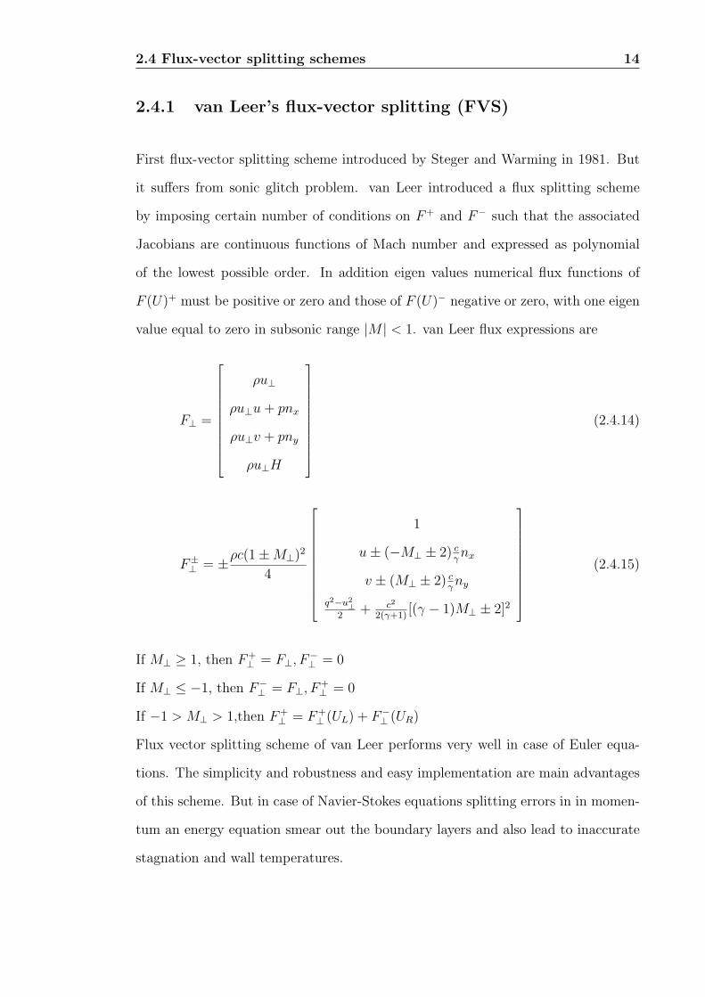
value equal to zero in subsonic range |M | < 1. van Leer flux expressions are
F⊥ =
ρu⊥
ρu⊥u + pnx
ρu⊥v + pny
ρu⊥H
(2.4.14)
F±⊥ = ±ρc(1±M⊥)2
4
1
u± (−M⊥ ± 2) cγnx
v ± (M⊥ ± 2) cγny
q2−u2⊥
2+ c2
2(γ+1)[(γ − 1)M⊥ ± 2]2
(2.4.15)
If M⊥ ≥ 1, then F+⊥ = F⊥, F−
⊥ = 0
If M⊥ ≤ −1, then F−⊥ = F⊥, F+
⊥ = 0
If −1 > M⊥ > 1,then F+⊥ = F+
⊥ (UL) + F−⊥ (UR)
Flux vector splitting scheme of van Leer performs very well in case of Euler equa-
tions. The simplicity and robustness and easy implementation are main advantages
of this scheme. But in case of Navier-Stokes equations splitting errors in in momen-
tum an energy equation smear out the boundary layers and also lead to inaccurate
stagnation and wall temperatures.
2.4 Flux-vector splitting schemes 15
2.4.2 Roe’s flux-difference splitting (FDS)
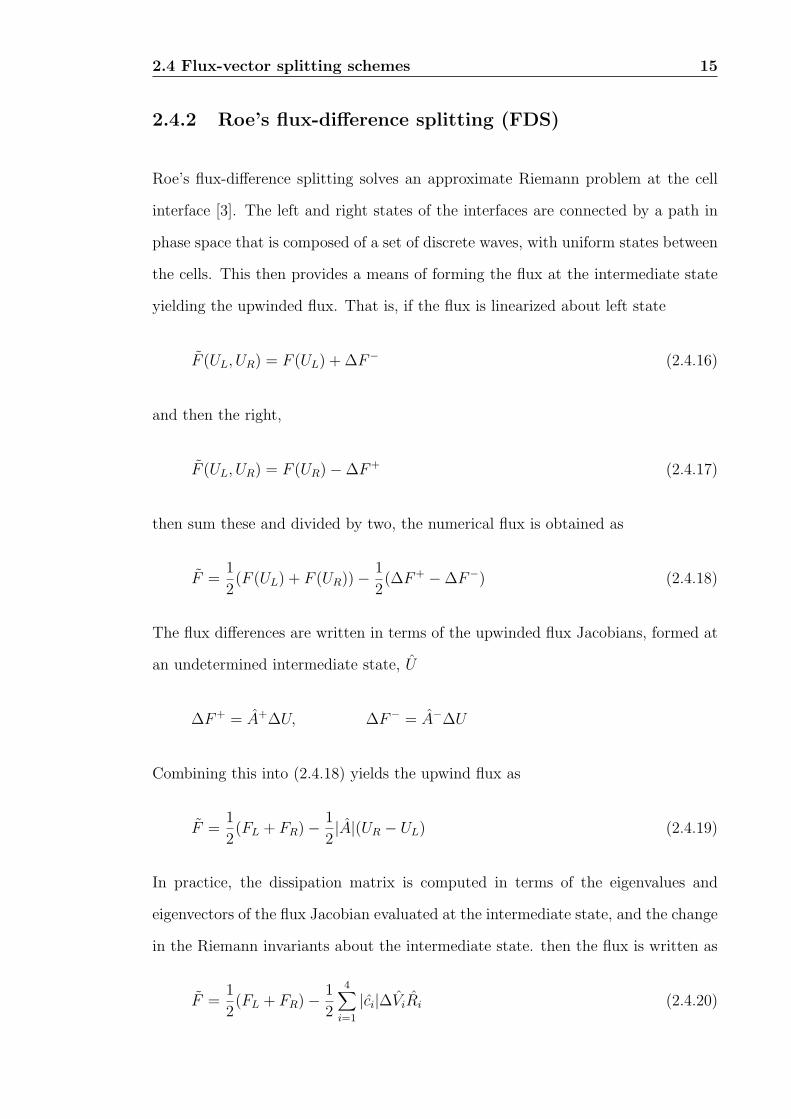
Roe’s flux-difference splitting solves an approximate Riemann problem at the cell
interface [3]. The left and right states of the interfaces are connected by a path in
phase space that is composed of a set of discrete waves, with uniform states between
the cells. This then provides a means of forming the flux at the intermediate state
yielding the upwinded flux. That is, if the flux is linearized about left state
F (UL, UR) = F (UL) + ∆F− (2.4.16)
and then the right,
F (UL, UR) = F (UR)−∆F+ (2.4.17)
then sum these and divided by two, the numerical flux is obtained as
F =1
2(F (UL) + F (UR))− 1
2(∆F+ −∆F−) (2.4.18)
The flux differences are written in terms of the upwinded flux Jacobians, formed at
an undetermined intermediate state, U
∆F+ = A+∆U, ∆F− = A−∆U
Combining this into (2.4.18) yields the upwind flux as
F =1
2(FL + FR)− 1
2|A|(UR − UL) (2.4.19)
In practice, the dissipation matrix is computed in terms of the eigenvalues and
eigenvectors of the flux Jacobian evaluated at the intermediate state, and the change
in the Riemann invariants about the intermediate state. then the flux is written as
F =1
2(FL + FR)− 1
2
4∑
i=1
|ci|∆ViRi (2.4.20)
2.4 Flux-vector splitting schemes 16
The intermediate state is formed as
ρ =√
ρLρR
u = uLω + uR(1− ω)
v = vLω + vR(1− ω)
H = HLω + HR(1− ω)
c = (γ − 1)(H − 12(u2 + v2))
where
ω =
√ρL√
ρL +√
ρR
The eigenvalues, λi, at the intermediate state are
λ =
uc − c
uc
uc
uc + c
While the change in the characteristic variables about the intermediate state, ∆Vi
are
∆Vi =
(∆P − ρc∆uc)2c2
ρ∆vc
c
∆ρ− ∆Pc2
(∆P + ρc∆uc)2c2
with ∆( ) = ( )R − ( )L. The acoustic eigenvalues, λ1,4 are modified to prevent
expansion shocks, yielding the ci as
c2,3 = λ2,3
2.4 Flux-vector splitting schemes 17
c1,4 =
|λ1,4| |λ1,4| ≥ 12δλ1,4
λ21,4
δλ1,4
+ 14δλ1,4 |λ1,4| < 1
2δλ1,4
(2.4.21)
where
δi = max(4(λi,R − λi,L), 0)
The columns of R are the right eigenvectors of A and are formed at the intermediate
state.
R =
1 0 1 1
u− nxc −ny c u u + nxc
v − ny c nxc v v + ny c
H − ucc vccu2
+v2
2H + ucc
(2.4.22)
This numerical flux has been proven to be robust, can capture strong, cell-aligned
shocks in one cell and, importantly, treats contact surfaces properly, yielding low
dissipation across shear and boundary layers. The implementation of this flux for
non-reacting, single component gases is relatively straight forward, but for reacting
or non-reacting flows of multi component gases the intermediate state is not unique,
and is costly to compute. Despite its few shortcomings, the numerical flux has
proven to be quite useful, and is probably the most used upwind flux formula today.
2.4.3 AUSM+
Liou and Steffen proposed AUSM for 2D Euler equations, in which the cell interface
advection Mach number is appropriately defined to determine the upwind extrapo-
lation for the convective quantities. AUSM+ [7] is designed to overcome the defect
of AUSM which is serious overshoots behind shock. The phenomena deteriorate
2.4 Flux-vector splitting schemes 18
convergence and increase grid dependency. AUSM+ is able to reduce this defect in
only shock aligned grids, no carbuncle phenomena, satisfaction of positivity condi-
tion, no oscillations at the slowly-moving shock, and efficiency. The AUSM+ can
be written at cell-interface as follows:
M1/2 = M+L /β= 1
8+ M−
R /β= 18
(2.4.23)
If (M1/2 ≥ 0)
F1/2AUSM+ = (M+L|β=1/8c 1
2φL+M−
R/β=1/8c 12φL)+(P+
L|α=3/16PL+P−R/α=3/16PR)(2.4.24)
Otherwise
F1/2AUSM+ = (M+L/β=1/8c 1
2φR+M−
R|β=1/8c 12φR)+(P+
L|α=3/16PL+P−R/α=3/16PR)(2.4.25)
Where
φ = [ρ ρu ρv ρH]T , P = P [0 nx ny 0]T
The split Mach number and the split pressure at the cell-interface of AUSM+ are
written as follows,
M±|β =
±14(M ± 1)2 ± β(M2 − 1)2 |M | ≤ 1
12(M ± |M |) |M | > 1
P± =
14(M ± 1)2(2∓M)± αM(M2 − 1)2 |M | ≤ 1
12(1± sign(M)) |M | > 1
The split Mach number and the speed of sound at the cell-interface of AUSM+ are
defined as follows,
ML,R =UL,R
c 12
, c 12
= min(cL, cR)
2.4 Flux-vector splitting schemes 19
Where
c =c2
max(|U |, c), c =
√√√√2(γ − 1)
(γ + 1)H
and U is the contravariant velocity
Chapter 3
Finite Volume Method
3.1 Introduction
The finite volume method was introduced into the field of numerical fluid dynamics
independently by McDonald in 1971 and McCromac and Paullay in 1972 for the so-
lution of two dimensional, time dependent Euler solutions. The 3D solution to Euler
equations given by Rizzi and Inouye in 1973. This name is given to the technique
by which the integral formulation of the conservative laws are discretized directly
in the physical space. Due to direct discretization of integral form of conservation
laws, the basic quantities mass, momentum and energy are conserved at the discrete
level. And there is no need of transformation of grids from one coordinate system
to another. FVM is very flexible. It can be implemented on structured as well as
unstructured grids. This renders FVM particularly suited for complex geometries.
FVM can be shown to be equivalent to a low order finite element method with less
numerical effort. Because of attractive properties of FVM this method is nowadays
very popular and in wide use.
3.2 The conservative discretization 21
3.2 The conservative discretization
Finite volume can be directly applied to integral form of governing equations .The
general form of conservation laws applied on a control volume Ω for scalar quantity
U and volume sources Q can be given as
∫ ∫ ∫
Ω
∂U
∂tdΩ +
∫ ∫ ∫
Ω(−→5.−→F ) dΩ =
∫
ΩQdΩ (3.2.1)
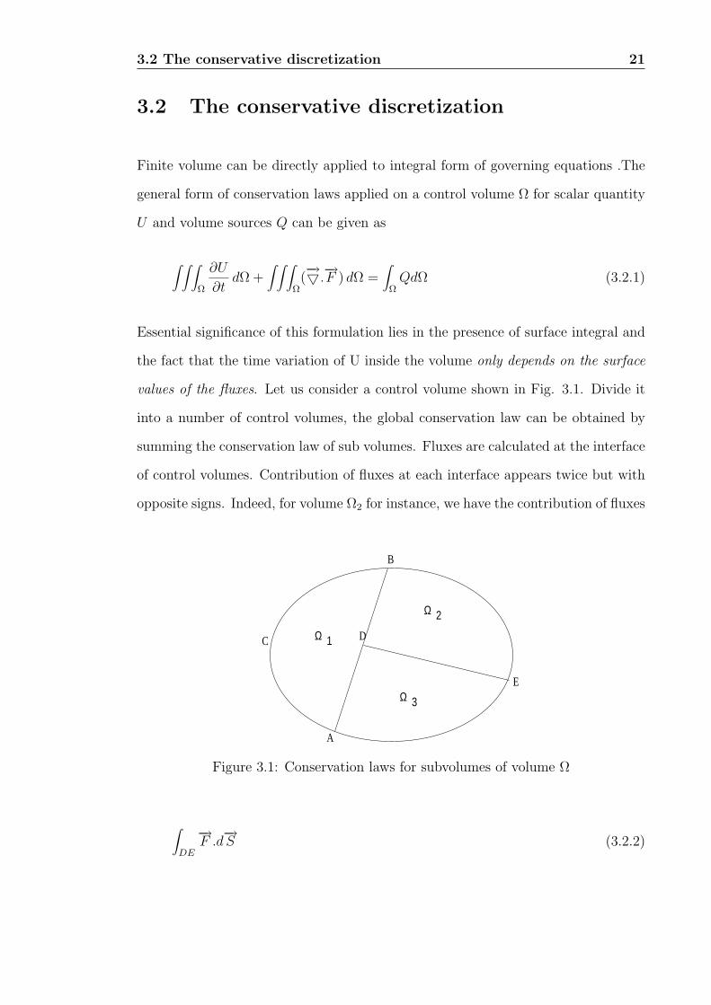
Essential significance of this formulation lies in the presence of surface integral and
the fact that the time variation of U inside the volume only depends on the surface
values of the fluxes. Let us consider a control volume shown in Fig. 3.1. Divide it
into a number of control volumes, the global conservation law can be obtained by
summing the conservation law of sub volumes. Fluxes are calculated at the interface
of control volumes. Contribution of fluxes at each interface appears twice but with
opposite signs. Indeed, for volume Ω2 for instance, we have the contribution of fluxes
A
B
C D
E
Ω
Ω
Ω 1
2
3
Figure 3.1: Conservation laws for subvolumes of volume Ω
∫
DE
−→F .d
−→S (3.2.2)
3.3 Finite volume method 22
while for Ω3 we have the similar term
∫
ED
−→F .d
−→S = −
∫
DE
−→F .d
−→S (3.2.3)
This is the essential property to be satisfied by numerical discretization of the flux
contributions, in order for scheme to be conservative.
3.3 Finite volume method
Basic concept of FVM is, the domain is subdivided into small cells (finite volumes).
The conservation equations in integral form are written for each of them separately.
Flux is required at the boundary of the control volume, which is a closed surface
in three dimensions and a closed contour in two dimensions. This flux must be
integrated to find the net flux through the boundary and source term also integrated
over the control volume to evaluate time variation of U inside the control volume.
Let us consider this approximation in more detail. We note that the average value
of U in the cell with volume Ω is
U =1
Ω
∫
ΩUdΩ (3.3.4)
and the discrete form of equation 3.2.1 can be written as
∂
∂t(UjΩj) +
∮F.dS = QjΩj (3.3.5)
In order to evaluate the fluxes, which are function of U , at the control volume
boundary, U can be represented within the cell by some piecewise approximation
which produces the correct value of U . This from of interpolation is often referred
to as reconstruction.
The basic elements of a FVM are thus the following:
3.4 Different frameworks in FVM 23
1. Given the value of U for each control volume, construct an approximation
to U(x, y, z) in each control volume. Using approximation, find U at each
control volume boundary. Evaluate F (U) at boundary. Since there is a distinct
approximation to U(x, y, z) in each control volume, two distinct values to the
flux will generally be obtained at any point on the boundary between two
control volumes.
2. Apply some strategy for resolving the discontinuity in the flux at control vol-
ume boundary to produce a single value of F (U) at any point on the boundary.
3. Integrate the flux to find the net flux through the control volume boundary
using some type of quadrature.
4. Advance the solution in time to obtain new values of U
3.4 Different frameworks in FVM
There are generally two discretization methods used in FVM which are cell centered
and cell vertex discretization. The two frameworks differ in location of control
volumes with respect to mesh and the location of the flow variable.
In cell centered scheme, flow quantities are stored at the centroid of grid cells. Thus,
control volumes are identical to the grid cells. When we evaluate the discretized flow
equations we have to supply convective and the viscous fluxes at the faces of the
cell. The fluxes are calculated by average of fluxes computed from the values at
centroids of the grid cells to the left and to the right of the cell face, but using
the same face vector(usually only for convective fluxes) or by using an average of
variables associated with the centroids of the grid cells to the left and to the right
of the cell face or reconstructed separately on both sides of cell face from the values
in the surrounding cells.
In cell vertex scheme, flow variables are stored at the grid points. The control volume
3.4 Different frameworks in FVM 24
(a) (b)
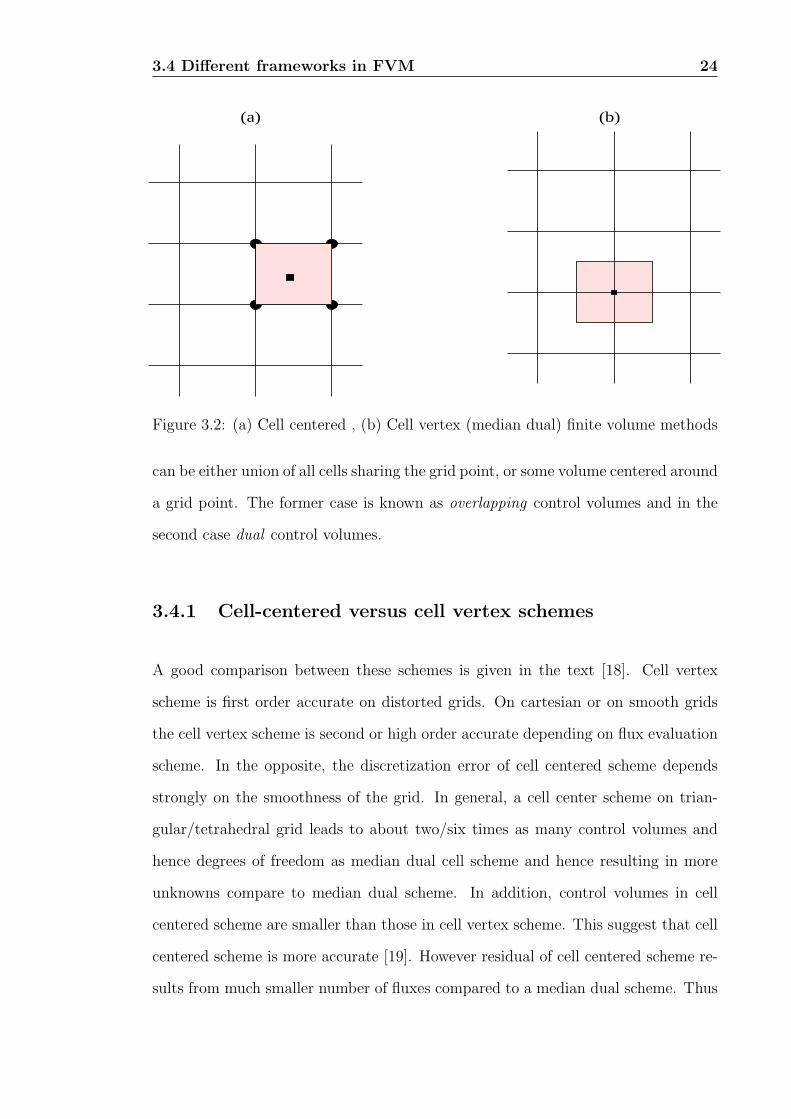
Figure 3.2: (a) Cell centered , (b) Cell vertex (median dual) finite volume methods
can be either union of all cells sharing the grid point, or some volume centered around
a grid point. The former case is known as overlapping control volumes and in the
second case dual control volumes.
3.4.1 Cell-centered versus cell vertex schemes
A good comparison between these schemes is given in the text [18]. Cell vertex
scheme is first order accurate on distorted grids. On cartesian or on smooth grids
the cell vertex scheme is second or high order accurate depending on flux evaluation
scheme. In the opposite, the discretization error of cell centered scheme depends
strongly on the smoothness of the grid. In general, a cell center scheme on trian-
gular/tetrahedral grid leads to about two/six times as many control volumes and
hence degrees of freedom as median dual cell scheme and hence resulting in more
unknowns compare to median dual scheme. In addition, control volumes in cell
centered scheme are smaller than those in cell vertex scheme. This suggest that cell
centered scheme is more accurate [19]. However residual of cell centered scheme re-
sults from much smaller number of fluxes compared to a median dual scheme. Thus
3.5 Discretization of N-S equations 25
there is no clear evidence about which scheme is better. Cell center schemes need
more computational work as ratio of number of faces to number of edges is more and
need more memory requirements as more number of variables to be stored compared
to cell vertex method. Boundary conditions implementation in cell vertex schemes
require additional logic in order to assure a consistent solution at boundary points
contrary to cell centered schemes; it is simple. In addition for cell vertex schemes
mass flux matrix treatment is required compare to cell centered scheme.
3.5 Discretization of N-S equations
Recall the conservation form of 2D Navier-Stokes equations
∂U
∂t+
∂(FI − FV )
∂x+
∂(GI −GV )
∂y= 0 (3.5.6)
the divergence form of N-S equation can be written as
Ut +∇.(−→F I −−→F V ) = 0 (3.5.7)
where
Ut =∂U
∂t(3.5.8)
−→FI = FI nx + GI ny
−→FV = FV nx + GV ny (3.5.9)
Integrating equation over a control volume Ωi (Fig. 3.3) and applying Gauss diver-
gence theorem to evaluate total flux, we have
∫
Ωi
UtdΩ +∮
ABC(−→F .n)dSi = 0 (3.5.10)
3.5 Discretization of N-S equations 26
. i
A
BC
D
Enk
nk
−
∆∆
S
∆ y
xk
1
Ω i
..3.
2.
. 4
X
Y
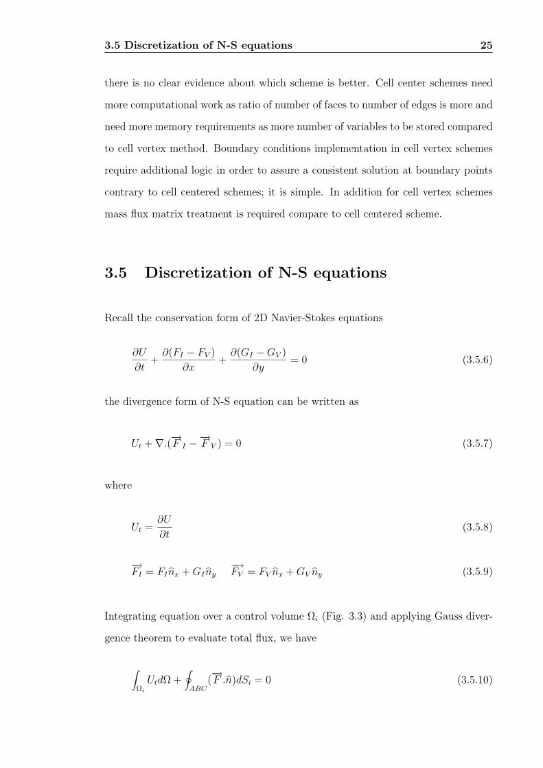
Figure 3.3: 2D finite volume method
n = ixny + iyny (3.5.11)
Where, nx = ∆ys
, ny = −∆xs
and i is the cell number, Si is boundary of control volume
Ωi. On integration, the space discrete form of N-S equations can be obtained as
dU
dt+
3∑
k=1
(FI⊥k − FV⊥k
).Sk = 0 (3.5.12)
k is the edge number. FI⊥k and FV⊥k represents normal flux on kth face with n as
the unit outward normal vector for viscous and inviscid fluxes respectively. Now we
arrive at the state update formula
Uin+1
= Uin − ∆t
Ωi
3∑
k=1
(FI⊥k − FV⊥k
).Sk = 0 (3.5.13)
where the normal flux vectors
FI⊥k =
ρu⊥k
ρuu⊥k + pnx,k
ρuu⊥k + pny,k
(p + e)u⊥k
(3.5.14)
3.5 Discretization of N-S equations 27
FV⊥k =
0
(τxx + τxy)nx,k
(τxy + τyy)ny,k
(uτxx + vτxy − qx)nx,k + (uτx,y + vτyy − qy)ny,k
(3.5.15)
3.5.1 Discretization of viscous fluxes
In order to find the viscous fluxes FV , the flow quantities and their first derivatives
in equation (3.5.15) are to be known at the faces of control volumes. Because of
elliptic nature of viscous fluxes, the values of velocity components u, v the dynamic
viscosity µ, which are required for the computation of viscous terms, are simply
averaged at face. Remaining task is evaluation of first derivatives of velocity and
1
a
m
2
3
4
Figure 3.4: Gradient computation at faces
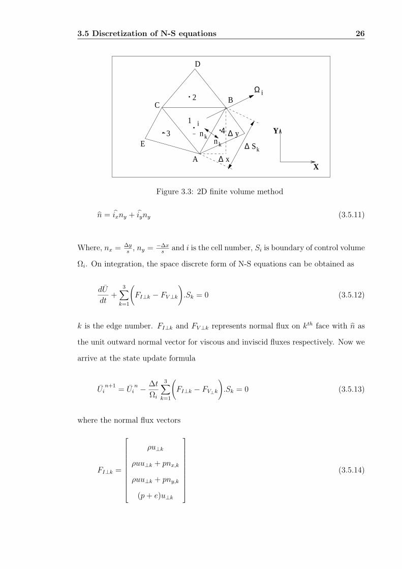
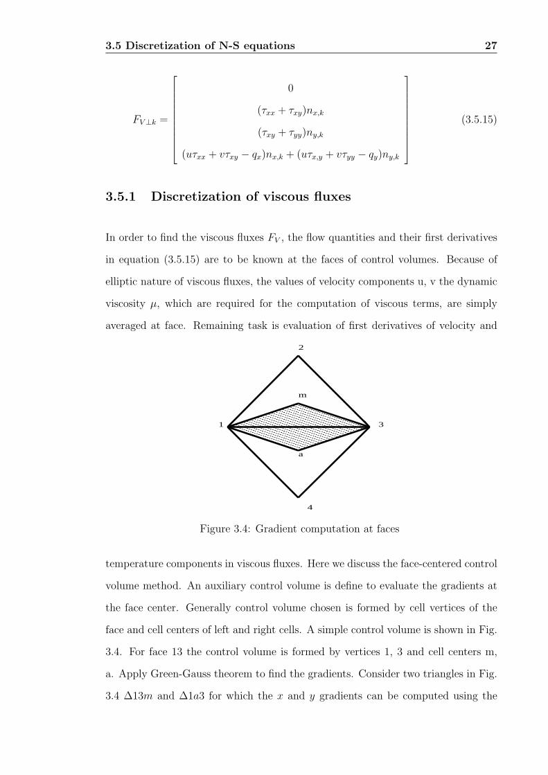
temperature components in viscous fluxes. Here we discuss the face-centered control
volume method. An auxiliary control volume is define to evaluate the gradients at
the face center. Generally control volume chosen is formed by cell vertices of the
face and cell centers of left and right cells. A simple control volume is shown in Fig.
3.4. For face 13 the control volume is formed by vertices 1, 3 and cell centers m,
a. Apply Green-Gauss theorem to find the gradients. Consider two triangles in Fig.
3.4 ∆13m and ∆1a3 for which the x and y gradients can be computed using the
3.6 Reconstruction and limiting 28
Green-Gauss theorem as
(Wx)13m =1
2A13m
[W1ym3 + Wmy31 + W3y1m] (3.5.16)
(Wy)13m = − 1
2A13m
[W1xm3 + Wmx31 + W3x1m] (3.5.17)
(Wx)1a3 =1
2A1a3
[W1y3a + W3ya1 + Way13] (3.5.18)
(Wy)1a3 = − 1
2A1a3
[W1x3a + W3xa1 + Wax13] (3.5.19)
Where ym3 = y3 − ym, xm3 = x3 − xm, and so on. The next step is to obtain the
face gradients. This is done using area-weighted average of these two gradients for
triangles 13m and 1a3:
(Wx)1a3m =[A13m(Wx)13m + A1a3(Wx)1a3]
[A13m + A1a3](3.5.20)
(Wy)1a3m =[A13m(Wy)13m + A1a3(Wy)1a3]
[A13m + A1a3](3.5.21)
3.6 Reconstruction and limiting
First order accurate results are obtained by assuming that the solution is constant
inside each control volume. We can achieve second or high order accuracy if we
assume the solution to vary over the control volumes. But it is not very easy to
obtain high order accuracy in FVM. If we extend first order upwind schemes by ap-
propriate second order accurate formulas, it leads to generation of oscillations near
discontinuities. A systematic analysis of the conditions required by a scheme to give
oscillation free solution was developed and initiated by Godunov, but it is proved to
be first order accurate. He introduced the important concept of monotonicity, which
3.6 Reconstruction and limiting 29
gives oscillation free solution. Monotonicity has the property of not allowing the
creation of new extrema and does not allow unphysical discontinuities. In order to
generate higher spacial approximation, the state variables at interface are obtained
from the extrapolation between neighboring cell averages. This method of genera-
tion of second order upwind schemes via variable extrapolation is often referred as
MUSCL (Monotone Upstream centered Scheme for Conservation Laws) introduced
by van Leer [5].
In constructing high order schemes the assumption of piecewise constant cell distri-
bution is replaced by linear distribution. To achieve high order accuracy unlike the
calculation of interface fluxes based on the cell average values in first order schemes,
flux has to be calculated based on point values on cell edges. For a given cell average
values, to find the point values using reconstruction procedure we require
1. Reconstruction for obtaining point values from cell averages.
2. Accurate quadrature formula for flux integral.
Starting with cell averaged data, the solution is piecewise linearly reconstructed such
that monotonicity condition preserved. The common cell edges, the reconstructed
values are not necessarily equal as both are reconstructed from different cell averages.
Thus there is a general discontinuity along common edges.
3.6.1 Multi-dimensional linear reconstruction of cell aver-
aged data
Higher order accuracy is obtained by performing piecewise linear reconstruction
of the cell averaged data. Here Barth [9] reconstruction procedure is presented.
Fig. 3.5 depicts the situation for a triangle A with neighboring triangles. Linear
3.6 Reconstruction and limiting 30
representation of state variables about a centroid (x0, y0) :
U(x, y) = U(x0, y0) + Ux(x− x0) + Uy(y − y0) = U(x0, y0) +−→∇U.∆−→r (3.6.22)
U(x0, y0) is cell average value given by state update formula equation (3.5.13). −→ris the distance vector,
−→∇U is the best estimate of the solution gradient in the cell
computed from the surrounding centroid data. Ux and Uy are the solution gradients
at each cell center. We can get high order solutions by estimating the gradients via,
1. Least-square reconstruction
2. Green-Gauss reconstruction
3. Frink’s higher order scheme
Least-square reconstruction
Least-square gradient reconstruction method originally formulated by Barth [10] for
the derivation of high-order upwind schemes. Consider the triangular mesh shown
in Fig. 3.5. Let xi and yi be the coordinates of node i and U(x0, y0) be the cell
average value. Now recall the equation (3.6.22)
Figure 3.5: 2D triangular mesh
3.6 Reconstruction and limiting 31
U(x, y) = U(x0, y0) + Ux.(x− x0) + Uy.(y − y0)
= U(x0, y0) +−→∇U.∆−→r
(3.6.23)
let
Ui = U(x, y)
U0 = U(x0, y0)
∆Ui = Ui − U0
∆xi = xi − x0
∆yi = yi − y0
Now the equation (3.6.23) becomes
∆Ui = Ux∆xi + Uy∆yi i = 1, 2, ...n. (3.6.24)
We have two unknowns Ux and Uy, and n linear equations. By minimizing the
square of the error.
error =n∑
i=1
(∆Ui − Ux∆xi + Uy∆yi)2 (3.6.25)
now we get least-square approximation of gradients as
Ux =||∆y||2(∆x, ∆U)− (∆x∆y)(∆y, ∆U)
||∆x||2||∆y||2 − (∆x1, ∆y)2(3.6.26)
Uy =||∆y||2(∆y, ∆U)− (∆x∆y)(∆x, ∆U)
||∆x||2||∆y||2 − (∆x1, ∆y)2(3.6.27)
Where,
||∆x||2 =∑n
i=1 ∆x2i , ||∆y||2 =
∑ni=1 ∆y2
i
(∆x, ∆U) =∑n
i=1 ∆xi∆Ui (∆y, ∆U) =∑n
i=1 ∆yi∆Ui
3.6 Reconstruction and limiting 32
Green-Gauss reconstruction
In this method gradients in the cell are calculated using Green’s theorem.
∫ ∫ ∫
Ω(−→5U) dΩ =
∫
S(U−→n ) ds (3.6.28)
The solution gradient for volume A is estimated by computing the boundary integral
of equation (3.6.28) for some path (surface) S, surrounding volume A.
−→5UA =1
Ω
∫
S(U−→n ) ds (3.6.29)
Frink’s high order scheme using Green-Gauss reconstruction
Frink [20] applied this reconstruction method to solve 3D Euler equation. First, The
gradients are evaluated using Green’s theorem as
Ux =1
Ω
∫UnydS (3.6.30)
Uy =1
Ω
∫UnxdS (3.6.31)
The above line integral is carried out around a closed path surrounding control
volume. First inverse distance weighing is used to transfer the cell average data to
the node as
Unode =
(N∑
i=1
Ui
ri
)/
(N∑
i=1
1
ri
)(3.6.32)
where ri is the distance from i-th cell center to the node of the cell and N is the
total number of cells sharing the particular node. unode and ui respectively denote
the values at the node and i-th cell center. Next, the trapezoidal rule is applied to
3.6 Reconstruction and limiting 33
integrate around the the control volume to compute the flow gradients. For example
x gradient is obtained by
Ux =1
Ω
K∑
i=1
(Unode1 + Unode2
2
)∆Sknx (3.6.33)
node1 and node2 are the end points of the cell face k, ∆S is the length of the cell face
k, nx is the x-component of the outward unit normal vector and K is the number
of cell edges of the control volume.
in two dimensions
ri = [(x0,i + xnode)2 + (y0,i + ynode)
2]0.5 (3.6.34)
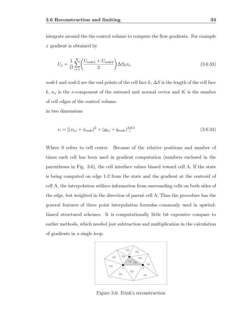
Where 0 refers to cell center. Because of the relative positions and number of
times each cell has been used in gradient computation (numbers enclosed in the
parentheses in Fig. 3.6), the cell interface values biased toward cell A. If the state
is being computed on edge 1-2 from the state and the gradient at the centroid of
cell A, the interpolation utilizes information from surrounding cells on both sides of
the edge, but weighted in the direction of parent cell A. Thus the procedure has the
general features of three point interpolation formulas commonly used in upwind-
biased structured schemes. It is computationally little bit expensive compare to
earlier methods, which needed just subtraction and multiplication in the calculation
of gradients in a single loop.
1
2
(1)(1)
(1)
(1)
(1)
(1)
(2)(2)
(2)
3
(1)
(3)"A"
Figure 3.6: Frink’s reconstruction
3.7 Quadratic-reconstruction 34
3.7 Quadratic-reconstruction
The fundamentals of the polynomial reconstructions to unstructured meshes for
building high order upwind schemes were presented first by Barth and Fredrickson
[10]. They attempted to extend to multiple dimensions some basic ideas previously
developed for structured meshes. The concept of polynomial reconstruction has
been applied to design essentially non-oscillatory schemes for unstructured meshes.
However, the computational effort associated with these complex methods through
the stencil selection turns out to be quite prohibitive for computing steady-state
solutions. Moreover, the nonlinearities inherent in these techniques may produce
serious convergence problems. For these reasons, Barth [11] introduced a simpler
quadratic reconstruction scheme with a fixed stencil in a cell vertex finite volume
solver. In the same way, a second-order finite volume solver that also preserves
quadratic polynomial has been proposed by Essers et al. for structured meshes.
This scheme suffers from a lack of conservation.
Our main objective is to develop a scheme whose second-order accuracy is preserved
even on much distorted meshes. Delanaye and Essers [12] developed a particular
form of quadratic reconstruction for the cell-centered scheme which is computation-
ally more efficient than the method of Barth. The flux balance is performed using
high order Gauss quadrature. An original quadratic reconstruction obtained by a
truncated Taylor-series expansion is employed to extrapolate the flow variables at
the quadrature points.
Outline of the method is the following. First, a multidimensional piecewise high or-
der polynomial approximates the flow variables evolution in the cell. The unknowns
of the control volume contour are computed. This step called as reconstruction, also
can be interpreted by extrapolation. On the each edge of the mesh, the advective
flux is obtained by applying a Riemann solver to reconcile the discontinuous left and
right states. Time evolution is then performed after correctly integrating the flux
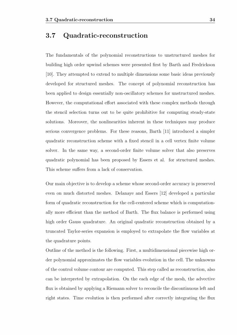
3.7 Quadratic-reconstruction 35
on the control volume contour. The spatial accuracy of the discretization depends
Quadrature points
P
P Parent Cell
Figure 3.7: The identification of more neighbors and flux integration path showedby dashed line
on two factors;
1) The accuracy of the variables reconstruction.
2) The flux integration.
The calculation of the flux through each edge fkn of a parent cell in Fig. 3.7 is per-
formed by a high order numerical integration of the flux functions using the n-points
Gauss quadrature;
fkn = δk
n∑
j=1
ωj[f(xkj , y
kj )nk
x + g(xkj , y
kj )nk
y] (3.7.35)
Where (xkj , y
kj ) are the coordinates of the Gauss quadrature point j and ωj denotes
the weight associated with this point. The lucid picture about the selection of Gauss
quadrature points on edges is provided in Appendix. By using n quadrature points,
the formula (3.7.35) allows the exact integration of polynomials with degree 2n-1.
Obviously, to satisfy the proposition, two quadrature points are at least required to
compute exactly a flux that is a quadratic polynomial of the Cartesian coordinates.
Two Riemann problems have therefore to be solved at each edge.
Right state at the quadrature point j of edge k is computed from
qkRj
= qkR + (rk
j − rkR)T∇qk
R +1
2(rk
j − rkR)T<R(rk
j − rkR) (3.7.36)
3.7 Quadratic-reconstruction 36
Where r is the position vector and < the Hessian matrix of each primitive variable:
< =
∂2xxq ∂2
xyq
∂2xyq ∂2
yyq
(3.7.37)
If q is a quadratic polynomial of x and y, equation (3.7.36) must be exact. That
requirement is met by equation (3.7.36) if the gradients and the second order deriva-
tives in the Hessian matrix are respectively computed with a second- and first-order
accuracy. This is accomplished by combining Green-Gauss gradient evaluation with
least-squares based approximation of the second derivatives, which leads to a numer-
ically efficient scheme. The technique we used to build second-order derivatives with
first-order accuracy is sometimes referred to as the minimum-energy reconstruction.
it simply consists in fitting a quadratic polynomial to the values of the neighbor-
ing nodes using the least-square technique. we seek to minimize the L2 norm of
the distance between a scalar function f known at the mesh nodes and a piecewise
quadratic approximation frec of the latter constructed as follows:
frec = fo + (r − ro)T∇fo +
1
2(r − ro)
T<o(r − ro) (3.7.38)
This is expressed by minimizing the functional
NΩ∑
i=1
[frec(ri)− fi]2 (3.7.39)
3.8 Limiters 37
and therefore, a NΩ X 5 linear system has to be solved for each control volume:
∆x1 ∆y1∆x2
1
2∆x1∆y1
∆y21
2
∆x2 ∆y2∆x2
2
2∆x2∆y2
∆y22
2
∆x3 ∆y3∆x2
3
2∆x3∆y3
∆y23
2
. . . . .
. . . . .
∆xi ∆yi∆x2
i
2∆xi∆yi
∆y2i
2
. . . . .
. . . . .
ux
uy
uxx
uxy
u− yy
=
∆u1
∆u2
∆u3
.
.
∆ui
.
.
(3.7.40)
where ∆ui = ui − u0
Finally, the quadratic reconstruction for a right state extrapolation
qkRj
= qkR + (rk
j−rkR)T∇1stqk
R + [−(rkj−rk
R)T ErR∇2qkR +
1
2(rk
j−rkR)T<R(rk
j−rkR)](3.7.41)
where ∇1st is a symbol notation for the numerical gradient calculated using Green-
Gaussian formula, ErR is 2 X 3 matrix containing constant coefficients of O(h) and
∇2 is the vector of second-order derivatives.
3.8 Limiters
Second and high order upwind discretization require use of limiters or limiting func-
tions in order to prevent the generation of oscillations and spurious solutions in the
region of high gradients (e.g., at shocks). A limiter is used to preserve monotonic-
ity principle, i.e., the reconstructed function must not exceed the maximum and
minimum of neighboring centroid values (including the centroid of parent cell) The
purpose of the limiter is to reduce the high gradient used to reconstruct the left
and right state at the face of the control volume in order to constrain the solution
3.8 Limiters 38
variation. At strong discontinuities, the limiter has to reduce slopes to zero to pre-
vent the generation of new extremum. We discuss the two limiters which are widely
using
1. Limiter of Barth and Jespersen
2. Venkatakrishnan limiter
Barth and Jespersen limiter
Consider the limited form of the reconstructed function about the centroid of triangle
A in Fig. 3.5.
U(x, y) = U(x0, y0) + φA−→∇UA.∆−→rA, φA ∈ [0, 1] (3.8.42)
the idea is to find the largest admissible φA. First compute UminA =min(UA, Uneighbors)
and UmaxA =max(UA, Uneighbors) then require that
UminA ≤ U(x, y)A ≤ Umax
A (3.8.43)
For cell centered method, Uneighbors are the number of cells sharing with common
edge of parent cell. For linear reconstruction, extrema in u(x, y)A occurs at the
vertices of the cell and the sufficient conditions stated in (3.8.43) can be easily
obtained. For each vertex of the cell compute Ui = U(xi, yi), i = 1, 2, 3..., d(c) to
determine the limited value, φA, which satisfies (3.8.43).
φA =
min(1,Umax
A −UA
Ui−UA), if Ui − UA > 0
min(1,Umin
A −UA
Ui−UA), if Ui − UA < 0
1 if Ui − UA = 0
(3.8.44)
3.8 Limiters 39
with φA=min( ¯φA1, ¯φA2, ¯φA3, ... ¯φAd(c)), ensures that the linearly reconstructed state
variables satisfy the monotonicity principle when evaluated anywhere within a cell.
Barth limiter ensures monotonicity, but it was shown to stall the convergence to
steady state [21], which could be due to the use of non-differentiable functions such
as max and min, apart from clipping smooth extrema.
Venkatakrishnan limiter
Venkatakrishnan limiter is widely used because of it’s superior convergence prop-
erties. It is based on Barth and Jesperson monotonicity principle on unstructured
grids. He modified the Van Albada limiter which is defined only for structured grids
and it is continuously differentiable. The limiter reduces the reconstructed gradient
∇U at cell center i by factor
φA =
1∆2
[(∆2
1,max+ε2)∆2+2∆22∆1,max
∆21,max+2∆2
2+∆1,max∆2+ε2
], if ∆2 > 0
1∆2
[(∆2
1,min+ε2)∆2+2∆22∆1,min
∆21,min+2∆2
2+∆1,min∆2+ε2
], if ∆2 < 0
1, if ∆2 = 0
(3.8.45)
Where
∆1,max = Umax − Ui
∆1,min = Umin − Ui
∆2 = Ui − UA
Umax, Umin values stand for the maximum and minimum values of all surrounding
cells which are shared by edges including cell i. Definitions of Umax and Umin are
same as explained in previous section. Parameter ε2 is intended to control the
amount of limiting . Setting ε2 to zero results in full limiting. Contrary to that, if ε2
set to large value, the limiter function will return a value of one. Hence, there will
3.8 Limiters 40
be no limiting at all and wiggles could occur in solution. In practice it was found
that ε2 should be proportional to a local length scale, i.e.,
ε2 = (K∆h)3 (3.8.46)
where K is a constant, and of order 1. ∆h is cube-root of the volume in 3D or
square root of area in 2D of the control volume. So far we have discussed Barth and
Jesperson [9] limiter and Venkatakrishnan [21] limiter. Venkatakrishnan’s limiter as
described in above section, helps in improving convergence characteristics of original
limiter, which however comes at the expense of compromising on monotonicity. Also
convergence seems to be strongly influenced by the parameter, which controls the
degree of limiting. This is function of an estimate of average grid size and a arbitrary
constant which is found after conducting experiments for each problem. This is a
limitation for Venkatakrishnan limiter to apply it in a general purpose problem.
In case of structured grids van Leer and van Albada limiters are quite success-
ful which are continuously diffentiable. Some attempts are made, to make some
changes to van Albada limiter to apply in unstructured grids. Indeed Venkatakrish-
nan limiter is modified form of van Albada limiter. One more attempt was made by
Van Rosendale [22] on triangular meshes, weighted average of gradients at the three
vertices of cell as computed by applying Green-Gauss theorem to surrounding cell
center data. The limited gradient within the cell obtained by taking the weighted
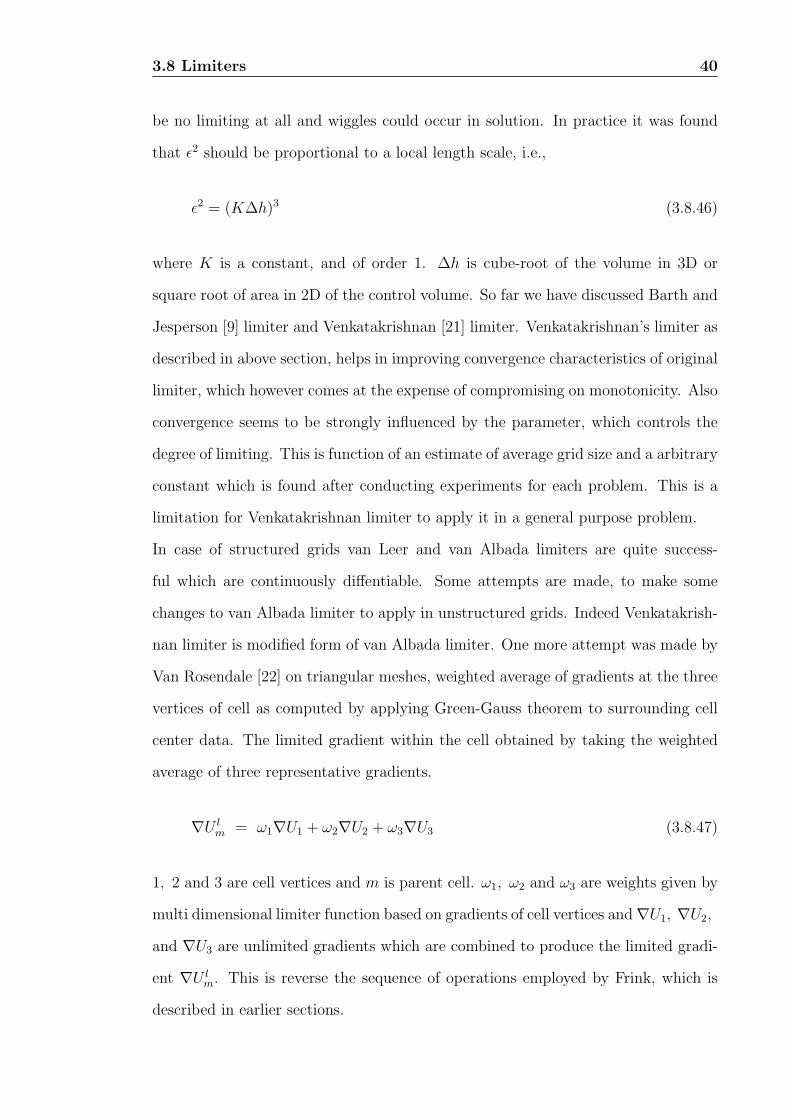
average of three representative gradients.
∇U lm = ω1∇U1 + ω2∇U2 + ω3∇U3 (3.8.47)
1, 2 and 3 are cell vertices and m is parent cell. ω1, ω2 and ω3 are weights given by
multi dimensional limiter function based on gradients of cell vertices and∇U1, ∇U2,
and ∇U3 are unlimited gradients which are combined to produce the limited gradi-
ent ∇U lm. This is reverse the sequence of operations employed by Frink, which is
described in earlier sections.
3.9 Jawahar and Kamath limiter 41
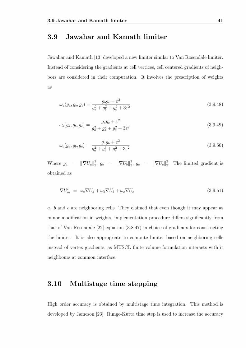
3.9 Jawahar and Kamath limiter
Jawahar and Kamath [13] developed a new limiter similar to Van Rosendale limiter.
Instead of considering the gradients at cell vertices, cell centered gradients of neigh-
bors are considered in their computation. It involves the prescription of weights
as
ωa(ga, gb, gc) =gbgc + ε2
g2a + g2
b + g2c + 3ε2
(3.9.48)
ωb(ga, gb, gc) =gagc + ε2
g2a + g2
b + g2c + 3ε2
(3.9.49)
ωc(ga, gb, gc) =gagb + ε2
g2a + g2
b + g2c + 3ε2
(3.9.50)
Where ga = ‖∇Ua‖22, gb = ‖∇Ub‖2
2, gc = ‖∇Uc‖22. The limited gradient is
obtained as
∇U lm = ωa∇Ua + ωb∇Ub + ωc∇Uc (3.9.51)
a, b and c are neighboring cells. They claimed that even though it may appear as
minor modification in weights, implementation procedure differs significantly from
that of Van Rosendale [22] equation (3.8.47) in choice of gradients for constructing
the limiter. It is also appropriate to compute limiter based on neighboring cells
instead of vertex gradients, as MUSCL finite volume formulation interacts with it
neighbours at common interface.
3.10 Multistage time stepping
High order accuracy is obtained by multistage time integration. This method is
developed by Jameson [23]. Runge-Kutta time step is used to increase the accuracy
3.11 Boundary conditions 42
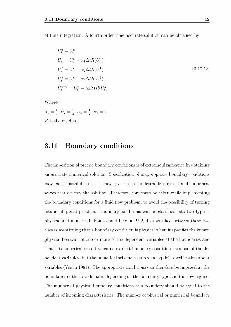
of time integration. A fourth order time accurate solution can be obtained by
U0i = Un
i
U1i = Un
i − α1∆tR(U0i )
U2i = Un
i − α2∆tR(U1i )
U3i = Un
i − α3∆tR(U2i )
Un+1i = Un
i − α4∆tR(U3i )
(3.10.52)
Where
α1 = 14
α2 = 13
α3 = 12
α4 = 1
R is the residual.
3.11 Boundary conditions
The imposition of precise boundary conditions is of extreme significance in obtaining
an accurate numerical solution. Specification of inappropriate boundary conditions
may cause instabilities or it may give rise to undesirable physical and numerical
waves that destroy the solution. Therefore, care must be taken while implementing
the boundary conditions for a fluid flow problem, to avoid the possibility of turning
into an ill-posed problem. Boundary conditions can be classified into two types -
physical and numerical. Poinsot and Lele in 1992, distinguished between these two
classes mentioning that a boundary condition is physical when it specifies the known
physical behavior of one or more of the dependent variables at the boundaries and
that it is numerical or soft when no explicit boundary condition fixes one of the de-
pendent variables, but the numerical scheme requires an explicit specification about
variables (Yee in 1981). The appropriate conditions can therefore be imposed at the
boundaries of the flow domain, depending on the boundary type and the flow regime.
The number of physical boundary conditions at a boundary should be equal to the
number of incoming characteristics. The number of physical or numerical boundary
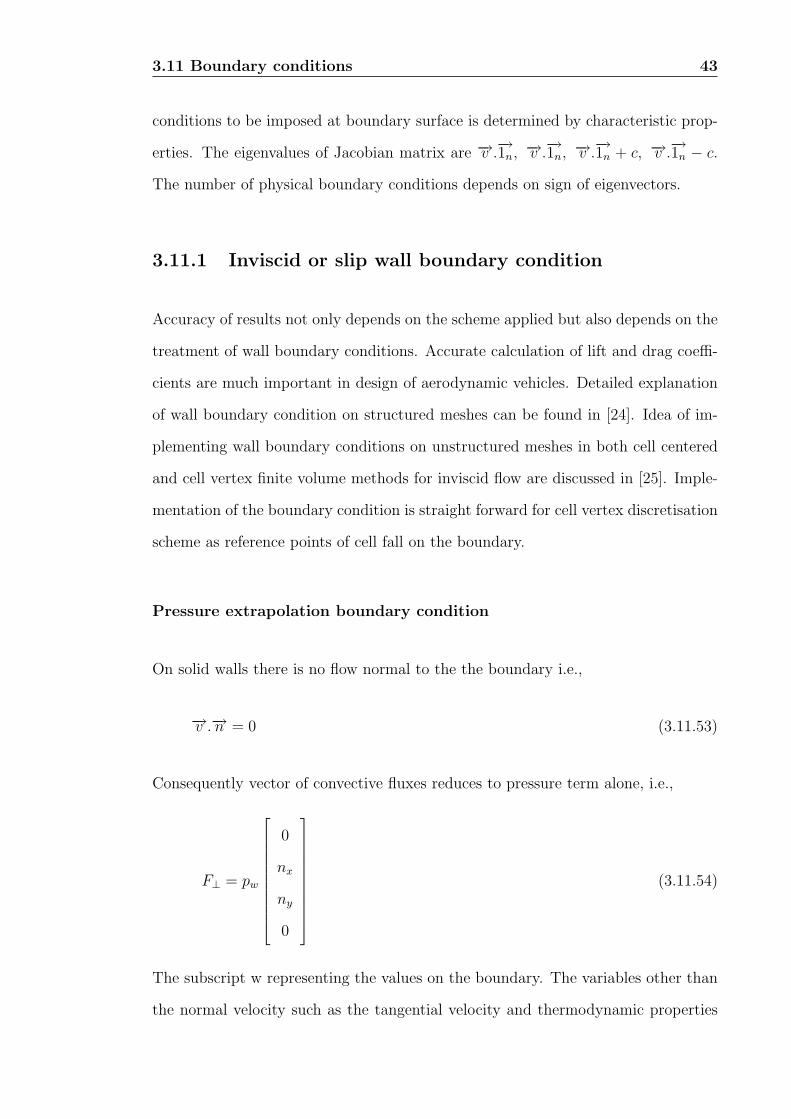
3.11 Boundary conditions 43
conditions to be imposed at boundary surface is determined by characteristic prop-
erties. The eigenvalues of Jacobian matrix are −→v .−→1n, −→v .
−→1n, −→v .
−→1n + c, −→v .
−→1n − c.
The number of physical boundary conditions depends on sign of eigenvectors.
3.11.1 Inviscid or slip wall boundary condition
Accuracy of results not only depends on the scheme applied but also depends on the
treatment of wall boundary conditions. Accurate calculation of lift and drag coeffi-
cients are much important in design of aerodynamic vehicles. Detailed explanation
of wall boundary condition on structured meshes can be found in [24]. Idea of im-
plementing wall boundary conditions on unstructured meshes in both cell centered
and cell vertex finite volume methods for inviscid flow are discussed in [25]. Imple-
mentation of the boundary condition is straight forward for cell vertex discretisation
scheme as reference points of cell fall on the boundary.
Pressure extrapolation boundary condition
On solid walls there is no flow normal to the the boundary i.e.,
−→v .−→n = 0 (3.11.53)
Consequently vector of convective fluxes reduces to pressure term alone, i.e.,
F⊥ = pw
0
nx
ny
0
(3.11.54)
The subscript w representing the values on the boundary. The variables other than
the normal velocity such as the tangential velocity and thermodynamic properties
3.11 Boundary conditions 44
such as total enthalpy or entropy are to be obtained from the interior flow. Pressure
pw can be obtained either by solving the momentum equation or by extrapolating
from the interior points. The former procedure will produce an artificial boundary
layer . A zero order extrapolation implies that the pressure at the reference point
itself is taken as the pressure at the boundary point, which is more justifiable in
case of cell-vertex finite volume formulation.
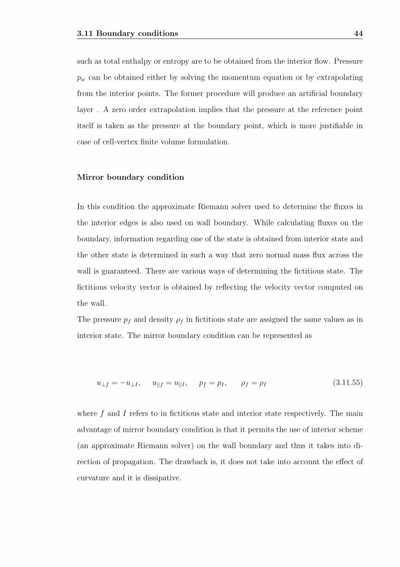
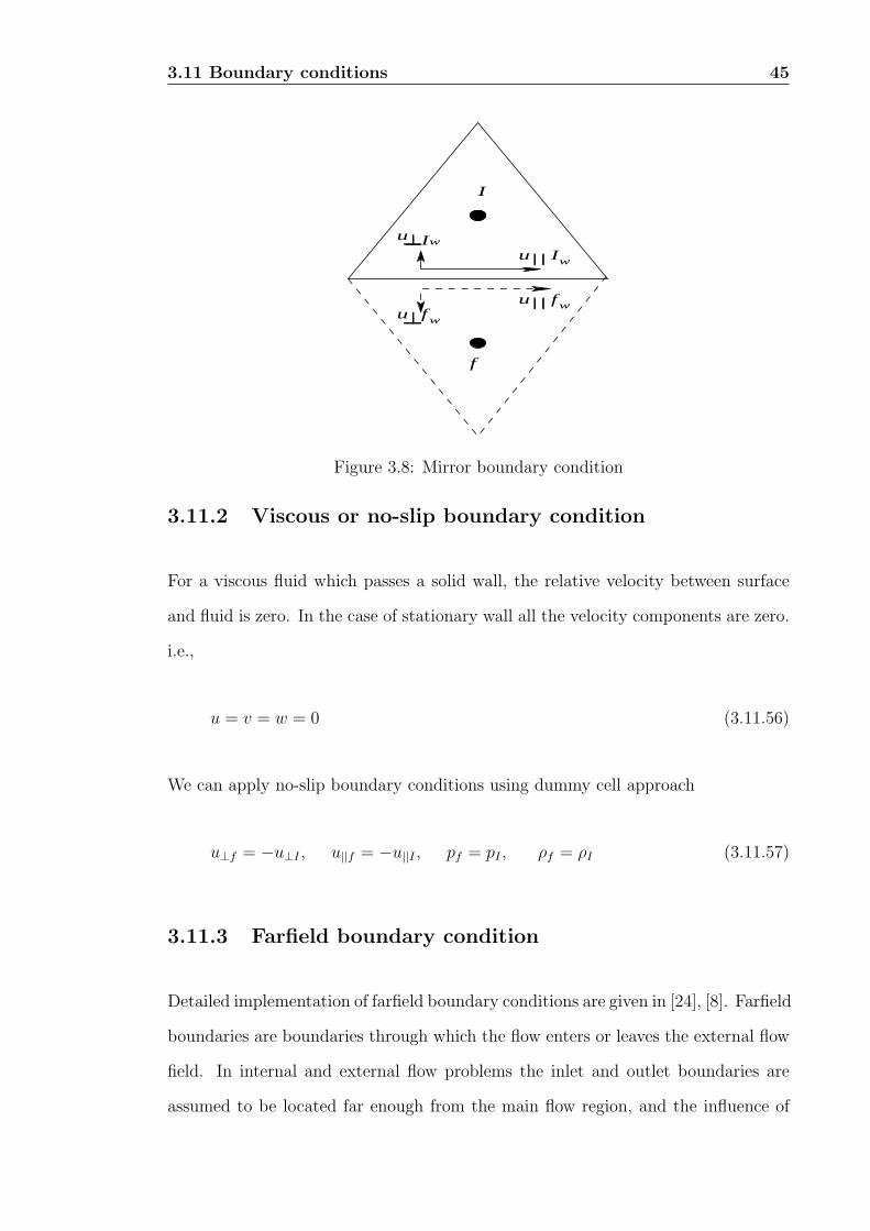
Mirror boundary condition
In this condition the approximate Riemann solver used to determine the fluxes in
the interior edges is also used on wall boundary. While calculating fluxes on the
boundary, information regarding one of the state is obtained from interior state and
the other state is determined in such a way that zero normal mass flux across the
wall is guaranteed. There are various ways of determining the fictitious state. The
fictitious velocity vector is obtained by reflecting the velocity vector computed on
the wall.
The pressure pf and density ρf in fictitious state are assigned the same values as in
interior state. The mirror boundary condition can be represented as
u⊥f = −u⊥I , u||f = u||I , pf = pI , ρf = ρI (3.11.55)
where f and I refers to in fictitious state and interior state respectively. The main
advantage of mirror boundary condition is that it permits the use of interior scheme
(an approximate Riemann solver) on the wall boundary and thus it takes into di-
rection of propagation. The drawback is, it does not take into account the effect of
curvature and it is dissipative.
3.11 Boundary conditions 45
I
uu
u w
fw
fw
IIu w
f
Figure 3.8: Mirror boundary condition
3.11.2 Viscous or no-slip boundary condition
For a viscous fluid which passes a solid wall, the relative velocity between surface
and fluid is zero. In the case of stationary wall all the velocity components are zero.
i.e.,
u = v = w = 0 (3.11.56)
We can apply no-slip boundary conditions using dummy cell approach
u⊥f = −u⊥I , u||f = −u||I , pf = pI , ρf = ρI (3.11.57)
3.11.3 Farfield boundary condition
Detailed implementation of farfield boundary conditions are given in [24], [8]. Farfield
boundaries are boundaries through which the flow enters or leaves the external flow
field. In internal and external flow problems the inlet and outlet boundaries are
assumed to be located far enough from the main flow region, and the influence of
3.11 Boundary conditions 46
the flow disturbances does not affect the freestream values. But high accuracy can
be achieved when we make some corrections on the farfield. The usual way of imple-
menting the farfield boundary conditions is using the information associated with
the Riemann invariants, given by
R1 = u⊥ +2c
γ − 1R2 = u⊥ − 2c
γ − 1R3 =
p
ργ(3.11.58)
These three Riemann invariants are associated with three waves with wave speeds of
u+c, u-c and u respectively. They remain constant as they enter or exit the farfield.
Depending on the value of the normal Mach number, Riemann invariants arriving
at a face on the farfield are determined based on left and right states. From these
Riemann invariants u⊥, p, ρ etc are determined on the face. These values are used
to find fluxes crossing the farfield.
3.11.4 Inflow/Outflow boundary conditions
Riemann invariants are calculated from known freestream values. So, farfield Bound-
ary condition are well suited for external flows as freestream condition are known. It
is not necessarily known all variables in case of internal flow. So, there is a separate
treatment of boundary conditions are required in the case of internal flow problems
Inflow boundary condition
Supersonic flow
All the eigenvalues are positive, therefore all four variables are fixed by physical
boundary conditions.
Subsonic flow
The direction normal to entry surface, Three eigenvalues are positive and one is
negative. Therefore three quantities will have to be fixed by physical boundary
3.11 Boundary conditions 47
conditions, while remaining one will be determined by interior conditions, through
numerical boundary condition.
Outflow boundary condition
Supersonic flow
All the eigenvalues are negative in sign, and no physical boundary conditions have
to be given. All boundary values are extrapolated from interior flow.
Subsonic flow
Three eigenvalues are negative, three numerical boundary conditions have to be
set, fourth one is specified by physical boundary conditions. The most appropriate
boundary condition for internal flows are fixing the downstream static pressure.
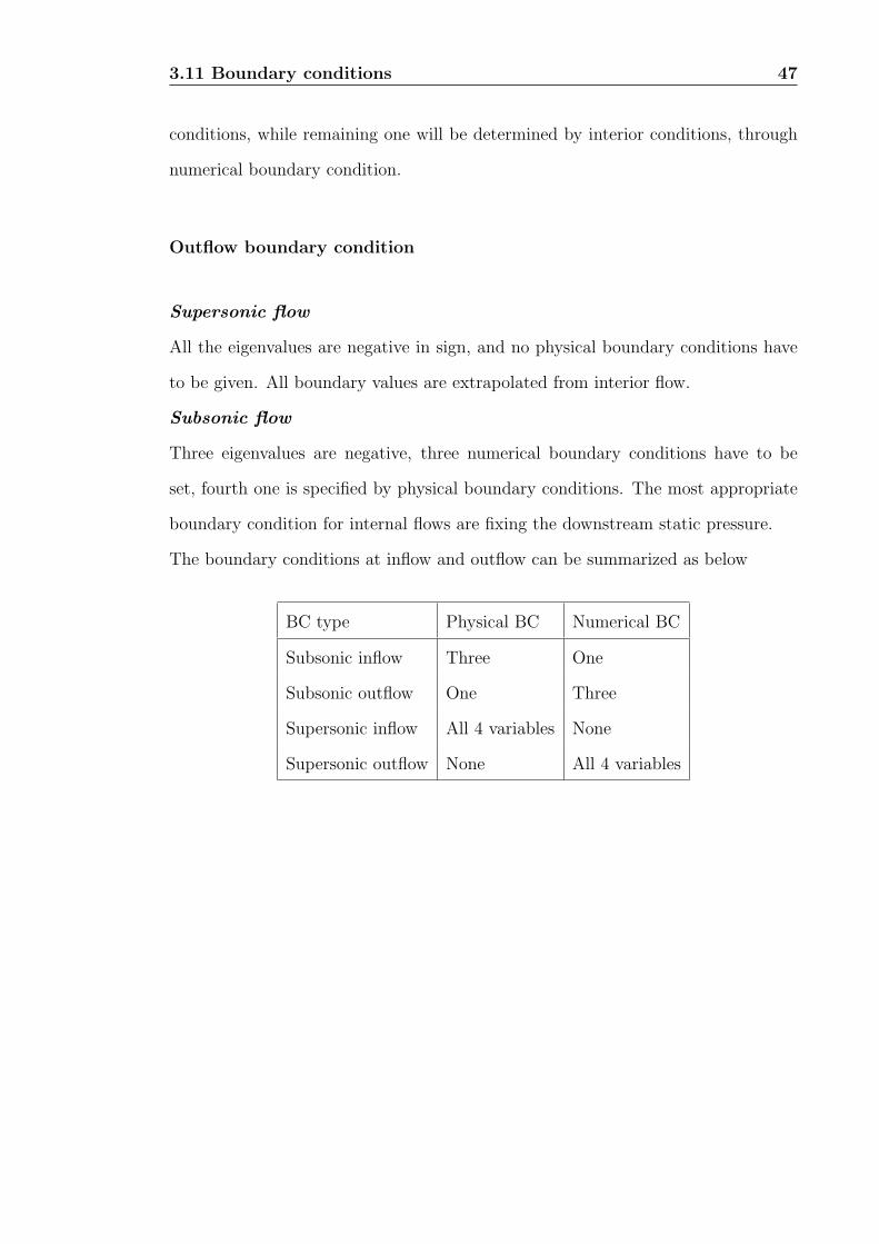
The boundary conditions at inflow and outflow can be summarized as below
BC type Physical BC Numerical BC
Subsonic inflow Three One
Subsonic outflow One Three
Supersonic inflow All 4 variables None
Supersonic outflow None All 4 variables
Chapter 4
Code Validation
The inviscid as well as the viscous part of the solver is validated by comparing with
various test cases results.
The inviscid code is validated for following test cases.
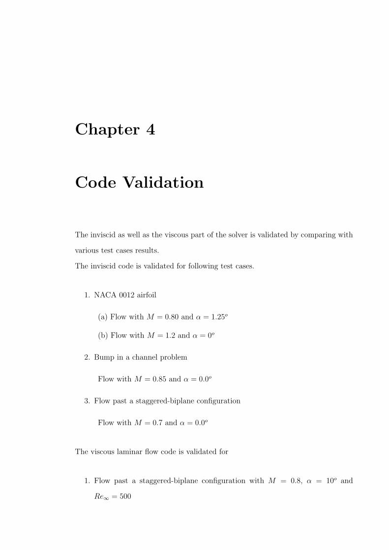
1. NACA 0012 airfoil
(a) Flow with M = 0.80 and α = 1.25o
(b) Flow with M = 1.2 and α = 0o
2. Bump in a channel problem
Flow with M = 0.85 and α = 0.0o
3. Flow past a staggered-biplane configuration
Flow with M = 0.7 and α = 0.0o
The viscous laminar flow code is validated for
1. Flow past a staggered-biplane configuration with M = 0.8, α = 10o and
Re∞ = 500
4.1 NACA 0012 airfoil 49
For all cases relative residual fall is computed using following relation
Residue = maximum||ρni − ρn−1
i ||/ρ1i 1 < i < nc (4.0.1)
In entropy contours, entropy is calculated using (p/ργ). Cp is calculated using
formula
Cp =P∞ − P
0.5ρ∞u2∞(4.0.2)
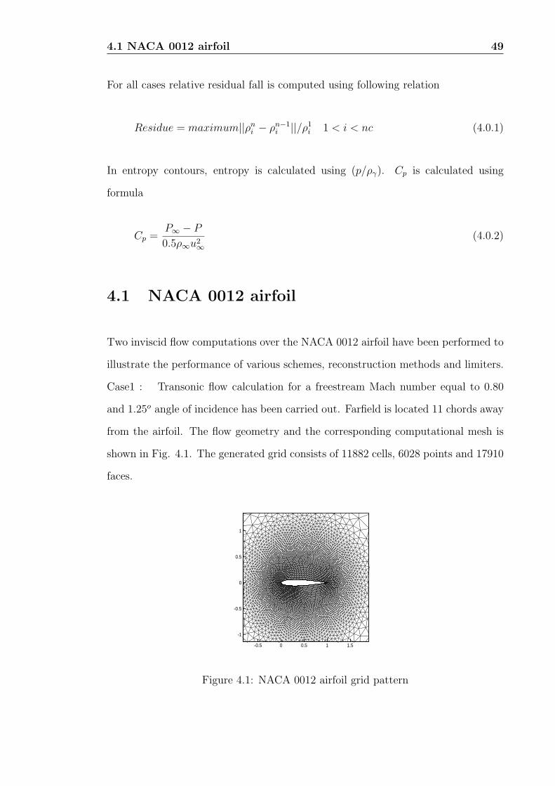
4.1 NACA 0012 airfoil
Two inviscid flow computations over the NACA 0012 airfoil have been performed to
illustrate the performance of various schemes, reconstruction methods and limiters.
Case1 : Transonic flow calculation for a freestream Mach number equal to 0.80
and 1.25o angle of incidence has been carried out. Farfield is located 11 chords away
from the airfoil. The flow geometry and the corresponding computational mesh is
shown in Fig. 4.1. The generated grid consists of 11882 cells, 6028 points and 17910
faces.
-0.5 0 0.5 1 1.5
-1
-0.5
0
0.5
1
Figure 4.1: NACA 0012 airfoil grid pattern
4.1 NACA 0012 airfoil 50
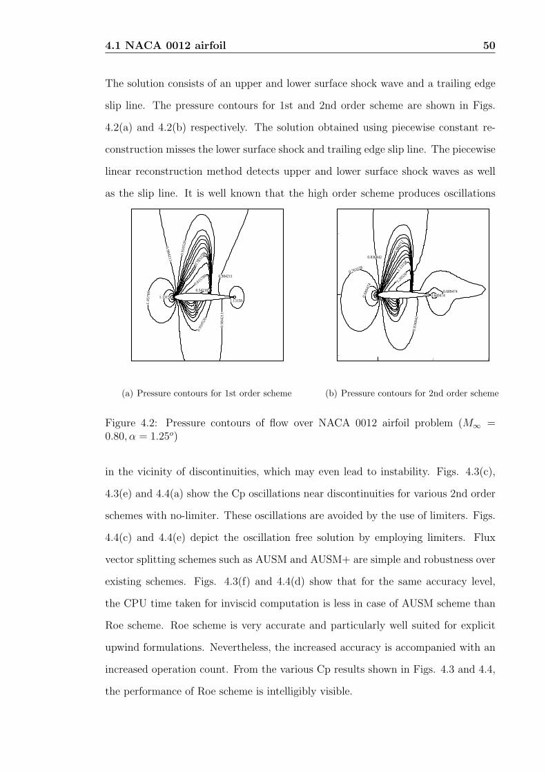
The solution consists of an upper and lower surface shock wave and a trailing edge
slip line. The pressure contours for 1st and 2nd order scheme are shown in Figs.
4.2(a) and 4.2(b) respectively. The solution obtained using piecewise constant re-
construction misses the lower surface shock and trailing edge slip line. The piecewise
linear reconstruction method detects upper and lower surface shock waves as well
as the slip line. It is well known that the high order scheme produces oscillations
1.05
789
1.13158
0.984211
0.91
0526
0.76
3158
0.615789
0.542105
0.984211
1.13158
0.98
4211
0.91
0526
(a) Pressure contours for 1st order scheme
0.68
9474
0.763158
0.836842
1.13
158
1.205
26
0.98
4211
0.83
6842
0.6894740.689474
(b) Pressure contours for 2nd order scheme
Figure 4.2: Pressure contours of flow over NACA 0012 airfoil problem (M∞ =0.80, α = 1.25o)
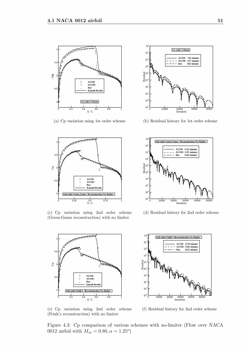
in the vicinity of discontinuities, which may even lead to instability. Figs. 4.3(c),
4.3(e) and 4.4(a) show the Cp oscillations near discontinuities for various 2nd order
schemes with no-limiter. These oscillations are avoided by the use of limiters. Figs.
4.4(c) and 4.4(e) depict the oscillation free solution by employing limiters. Flux
vector splitting schemes such as AUSM and AUSM+ are simple and robustness over
existing schemes. Figs. 4.3(f) and 4.4(d) show that for the same accuracy level,
the CPU time taken for inviscid computation is less in case of AUSM scheme than
Roe scheme. Roe scheme is very accurate and particularly well suited for explicit
upwind formulations. Nevertheless, the increased accuracy is accompanied with an
increased operation count. From the various Cp results shown in Figs. 4.3 and 4.4,
the performance of Roe scheme is intelligibly visible.
4.1 NACA 0012 airfoil 51
...
.
....
.
.
.
..
.........
...
. .
.
. . . . . . .
......
..............
............................
..
.. . . . . . . . . . . . . . . . . . .
..........
X / C
-C
p
0 0.2 0.4 0.6 0.8 1
-1
-0.5
0
0.5
1
AUSMAUSM+RoeKamath Results
.
1st order Scheme
(a) Cp variation using 1st order scheme
Iterations
Res
idua
l
0 10000 20000 30000 4000010-9
10-8
10-7
10-6
10-5
10-4
10-3
10-2
10-1
100
AUSM 742 minutesAUSM+ 677 minutesRoe 843 minutes
1st order Scheme
(b) Residual history for 1st order scheme
...
.
.
..
.
.
.
...
........
....
. . .
.
.. . . . .
....................
............................
..
.. . . . . . . . . . . . . . . . . . .
..........
X / C
-Cp
0 0.25 0.5 0.75 1
-1
-0.5
0
0.5
1
AUSMAUSM+RoeKamath Results
.
2nd order Green-Gauss Reconstruction No-limiter
(c) Cp variation using 2nd order scheme(Green-Gauss reconstruction) with no limiter
Iterations
Res
idua
l
0 10000 20000 30000 40000 5000010-9
10-8
10-7
10-6
10-5
10-4
10-3
10-2
10-1
100
AUSM 1142 minutesAUSM+ 1135 minutesRoe 1244 minutes
2nd order Green-Gauss Reconstruction No-limiter
(d) Residual history for 2nd order scheme
...
.
.
..
.
.
.
...
........
....
. . .
.
.. . . . .
....
................
............................
..
.. . . . . . . . . . . . . . . . . . .
..........
X / C
-Cp
0 0.2 0.4 0.6 0.8 1
-1
-0.5
0
0.5
1
AUSMAUSM+Roekamath Results
.
2nd order Frink’s Reconstruction No-limiter
(e) Cp variation using 2nd order scheme(Frink’s reconstruction) with no limiter
Iterarions
Res
idua
l
0 10000 20000 30000 40000 5000010-9
10-8
10-7
10-6
10-5
10-4
10-3
10-2
10-1
100
AUSM 1578 minutesAUSM+ 1582 minutesRoe 1625 minutes
2nd order Frink’s Reconstruction No-limiter
(f) Residual history for 2nd order scheme
Figure 4.3: Cp comparison of various schemes with no-limiter (Flow over NACA0012 airfoil with M∞ = 0.80, α = 1.25o)
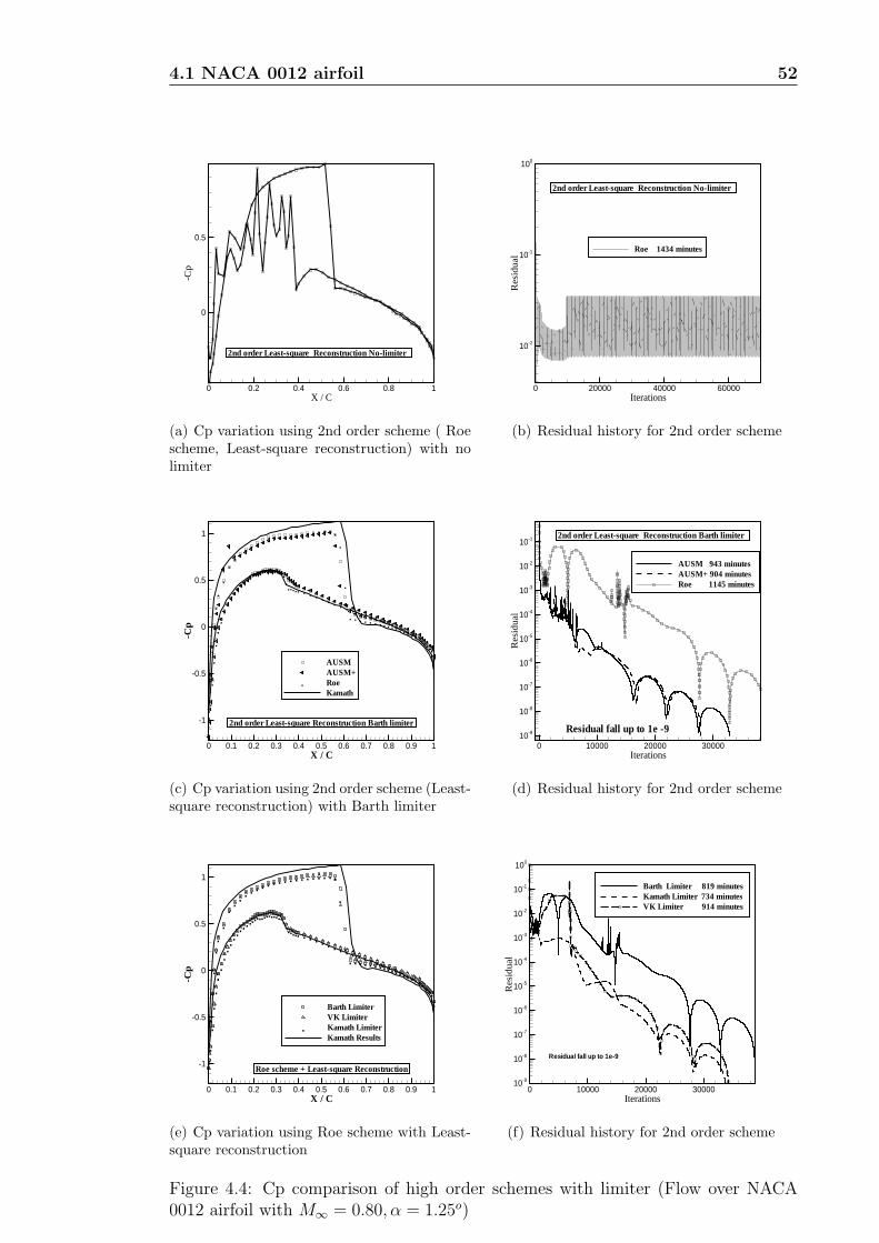
4.1 NACA 0012 airfoil 52
X / C
-Cp
0 0.2 0.4 0.6 0.8 1
0
0.5
2nd order Least-square Reconstruction No-limiter
(a) Cp variation using 2nd order scheme ( Roescheme, Least-square reconstruction) with nolimiter
Iterations
Res
idua
l
0 20000 40000 60000
10-2
10-1
100
Roe 1434 minutes
2nd order Least-square Reconstruction No-limiter
(b) Residual history for 2nd order scheme
..
.
.
...
.
.
.
.
..
.........
...
..
.
. . . . . . .
.........
...........
..........................
..
..
.
.. . . . . . . . . . . . . . . . . .
. . . . . . . . . .
X / C
-Cp
0 0.1 0.2 0.3 0.4 0.5 0.6 0.7 0.8 0.9 1
-1
-0.5
0
0.5
1
AUSMAUSM+RoeKamath
.
2nd order Least-square Reconstruction Barth limiter
(c) Cp variation using 2nd order scheme (Least-square reconstruction) with Barth limiter
Iterations
Res
idua
l
0 10000 20000 3000010-9
10-8
10-7
10-6
10-5
10-4
10-3
10-2
10-1
AUSM 943 minutesAUSM+ 904 minutesRoe 1145 minutes
Residual fall up to 1e -9
2nd order Least-square Reconstruction Barth limiter
(d) Residual history for 2nd order scheme
...
.
....
.
.
.
..
.........
...
.
.
.. . . . . . .
......
..............
...........................
..
.
.. . . . . . . . . . . . . . . . . . .
..........
X / C
-Cp
0 0.1 0.2 0.3 0.4 0.5 0.6 0.7 0.8 0.9 1
-1
-0.5
0
0.5
1
Barth LimiterVK LimiterKamath LimiterKamath Results
.
Roe scheme + Least-square Reconstruction
(e) Cp variation using Roe scheme with Least-square reconstruction
Iterations
Res
idua
l
0 10000 20000 3000010-9
10-8
10-7
10-6
10-5
10-4
10-3
10-2
10-1
100
Barth Limiter 819 minutesKamath Limiter 734 minutesVK Limiter 914 minutes
Residual fall up to 1e-9
(f) Residual history for 2nd order scheme
Figure 4.4: Cp comparison of high order schemes with limiter (Flow over NACA0012 airfoil with M∞ = 0.80, α = 1.25o)
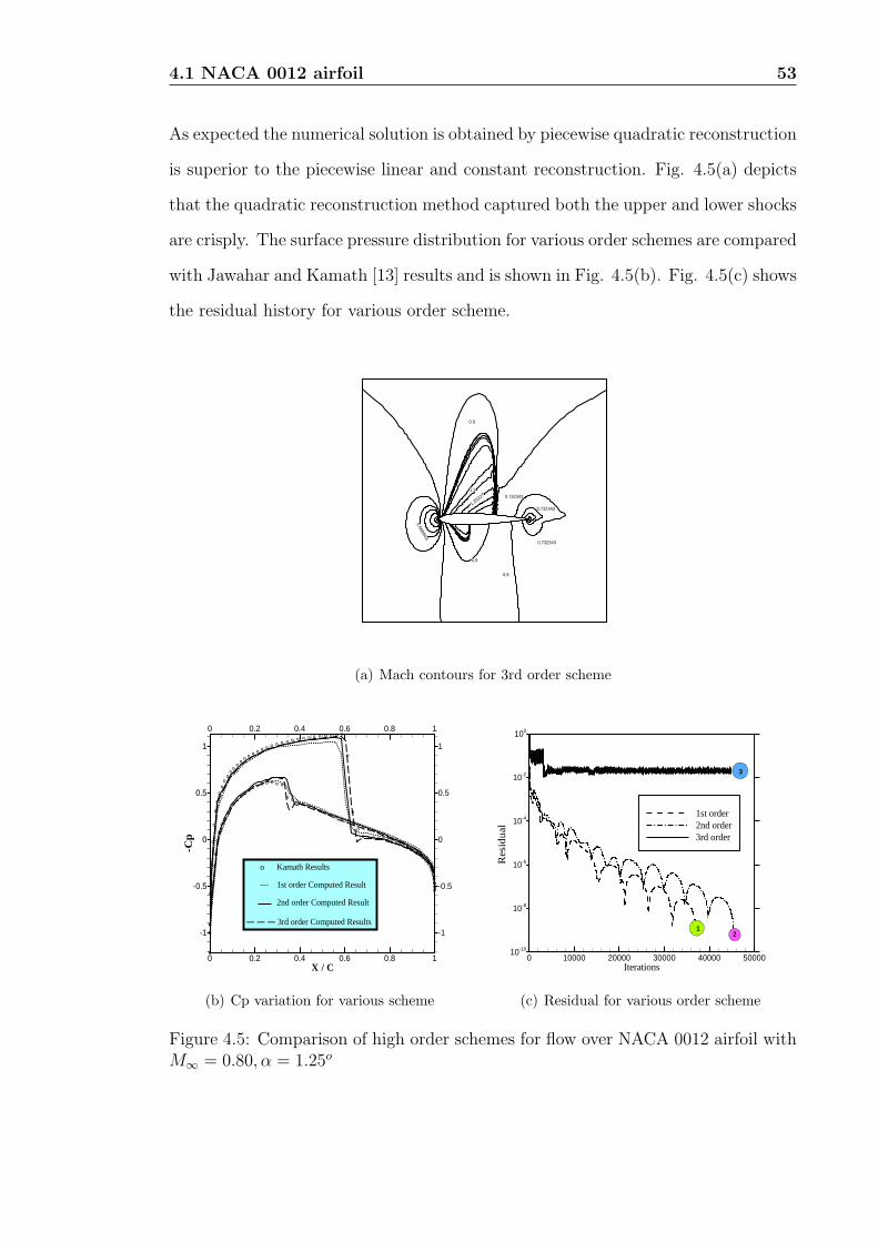
4.1 NACA 0012 airfoil 53
As expected the numerical solution is obtained by piecewise quadratic reconstruction
is superior to the piecewise linear and constant reconstruction. Fig. 4.5(a) depicts
that the quadratic reconstruction method captured both the upper and lower shocks
are crisply. The surface pressure distribution for various order schemes are compared
with Jawahar and Kamath [13] results and is shown in Fig. 4.5(b). Fig. 4.5(c) shows
the residual history for various order scheme.
0.688943
1.2
1.26227
0.9
0.732343
0.732343
0.732343
0.8
0.9
(a) Mach contours for 3rd order scheme
O
O
O
O
O
O
O
O
O
O
O
OO
OO
OO
OO
O OO O O O O O O O O O O O O O O O
O
O
O
O O O O O O O O O O O OOOOO
OO
OOOOOOOO
O
O
O
O
O
O
O
O
O
O
OO
OO
OO
OO
O O O O O O O
OO
O OO
O OO O O O
O O O O O O O O O O OO O
O O OOOO
OOOOOOOOOO
X / C
-Cp
00
0
0.20.2
0.2
0.40.4
0.4
0.60.6
0.6
0.80.8
0.8
11
1
-1-1 -1
-0.5-0.5 -0.5
00 0
0.50.5 0.5
11 1
o Kamath Results
--- 1st order Computed Result
2nd order Computed Result
_ _ _ 3rd order Computed Results
(b) Cp variation for various scheme
Iterations
Res
idua
l
0 10000 20000 30000 40000 5000010-10
10-8
10-6
10-4
10-2
100
1st order2nd order3rd order
12
3
(c) Residual for various order scheme
Figure 4.5: Comparison of high order schemes for flow over NACA 0012 airfoil withM∞ = 0.80, α = 1.25o
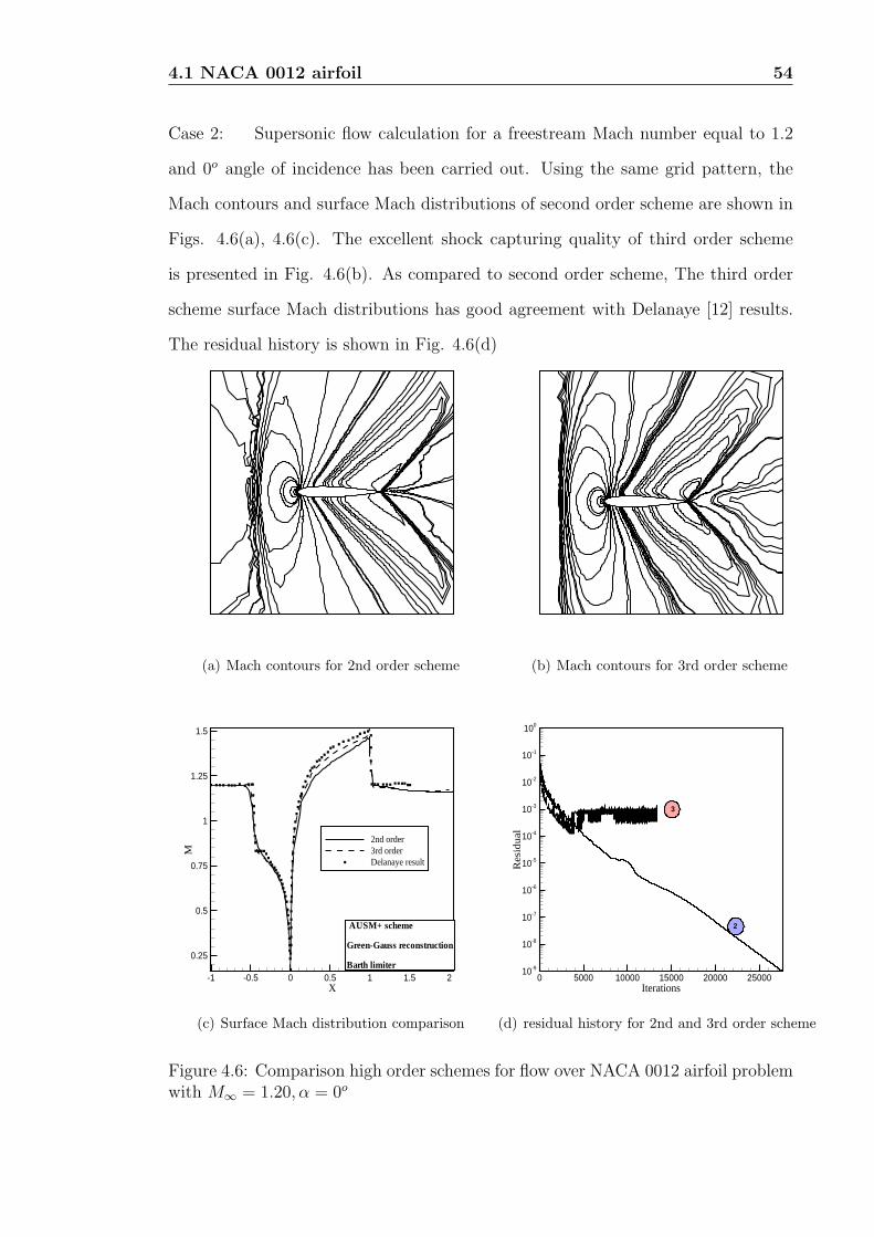
4.1 NACA 0012 airfoil 54
Case 2: Supersonic flow calculation for a freestream Mach number equal to 1.2
and 0o angle of incidence has been carried out. Using the same grid pattern, the
Mach contours and surface Mach distributions of second order scheme are shown in
Figs. 4.6(a), 4.6(c). The excellent shock capturing quality of third order scheme
is presented in Fig. 4.6(b). As compared to second order scheme, The third order
scheme surface Mach distributions has good agreement with Delanaye [12] results.
The residual history is shown in Fig. 4.6(d)
(a) Mach contours for 2nd order scheme (b) Mach contours for 3rd order scheme
X
M
-1 -0.5 0 0.5 1 1.5 2
0.25
0.5
0.75
1
1.25
1.5
2nd order3rd orderDelanaye result
AUSM+ scheme
Green-Gauss reconstruction
Barth limiter
(c) Surface Mach distribution comparison
Iterations
Res
idua
l
0 5000 10000 15000 20000 2500010-9
10-8
10-7
10-6
10-5
10-4
10-3
10-2
10-1
100
3
2
(d) residual history for 2nd and 3rd order scheme
Figure 4.6: Comparison high order schemes for flow over NACA 0012 airfoil problemwith M∞ = 1.20, α = 0o
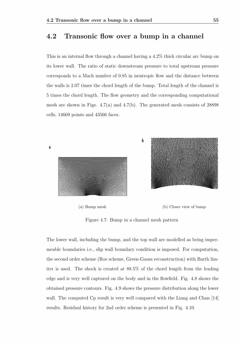
4.2 Transonic flow over a bump in a channel 55
4.2 Transonic flow over a bump in a channel
This is an internal flow through a channel having a 4.2% thick circular arc bump on
its lower wall. The ratio of static downstream pressure to total upstream pressure
corresponds to a Mach number of 0.85 in isentropic flow and the distance between
the walls is 2.07 times the chord length of the bump. Total length of the channel is
5 times the chord length. The flow geometry and the corresponding computational
mesh are shown in Figs. 4.7(a) and 4.7(b). The generated mesh consists of 28898
cells, 14669 points and 43566 faces.
a
(a) Bump mesh
b
(b) Closer view of bump
Figure 4.7: Bump in a channel mesh pattern
The lower wall, including the bump, and the top wall are modelled as being imper-
meable boundaries i.e., slip wall boundary condition is imposed. For computation,
the second order scheme (Roe scheme, Green-Gauss reconstruction) with Barth lim-
iter is used. The shock is created at 88.5% of the chord length from the leading
edge and is very well captured on the body and in the flowfield. Fig. 4.8 shows the
obtained pressure contours. Fig. 4.9 shows the pressure distribution along the lower
wall. The computed Cp result is very well compared with the Liang and Chan [14]
results. Residual history for 2nd order scheme is presented in Fig. 4.10.
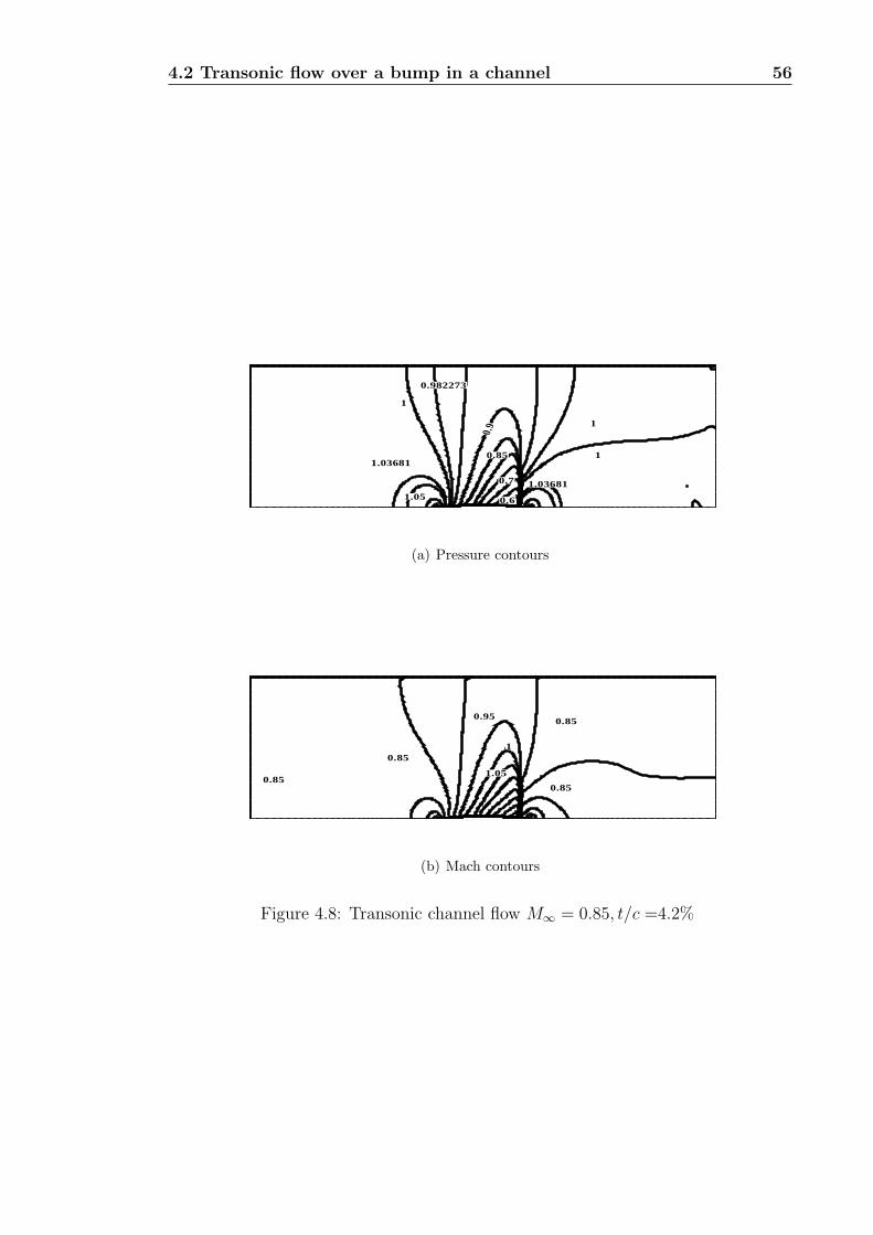
4.2 Transonic flow over a bump in a channel 56
1
0.9
0.85
0.7
0.6
1.03681
1
11.03681
1.05
0.982273
(a) Pressure contours
0.85
0.95
1
0.850.85
0.85
1.05
(b) Mach contours
Figure 4.8: Transonic channel flow M∞ = 0.85, t/c =4.2%
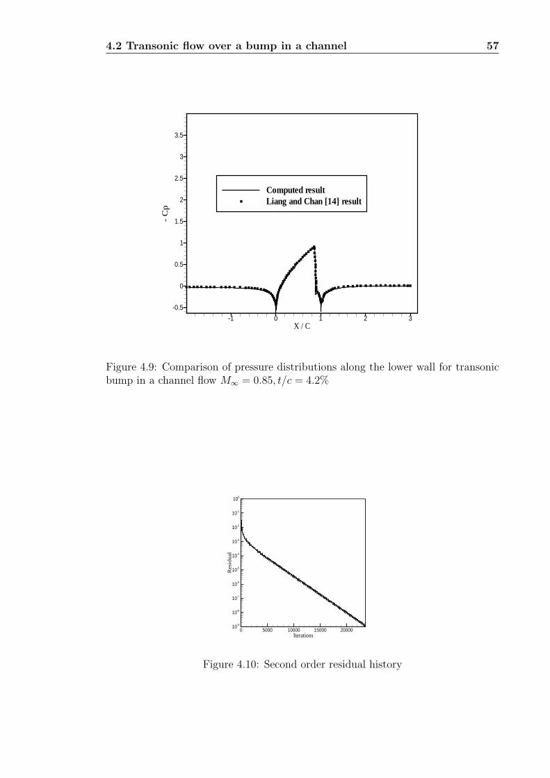
4.2 Transonic flow over a bump in a channel 57
X / C
-C
p
-1 0 1 2 3
-0.5
0
0.5
1
1.5
2
2.5
3
3.5
Computed resultLiang and Chan [14] result
Figure 4.9: Comparison of pressure distributions along the lower wall for transonicbump in a channel flow M∞ = 0.85, t/c = 4.2%
Iterations
Res
idu
al
0 5000 10000 15000 2000010-9
10-8
10-7
10-6
10-5
10-4
10-3
10-2
10-1
100
Figure 4.10: Second order residual history
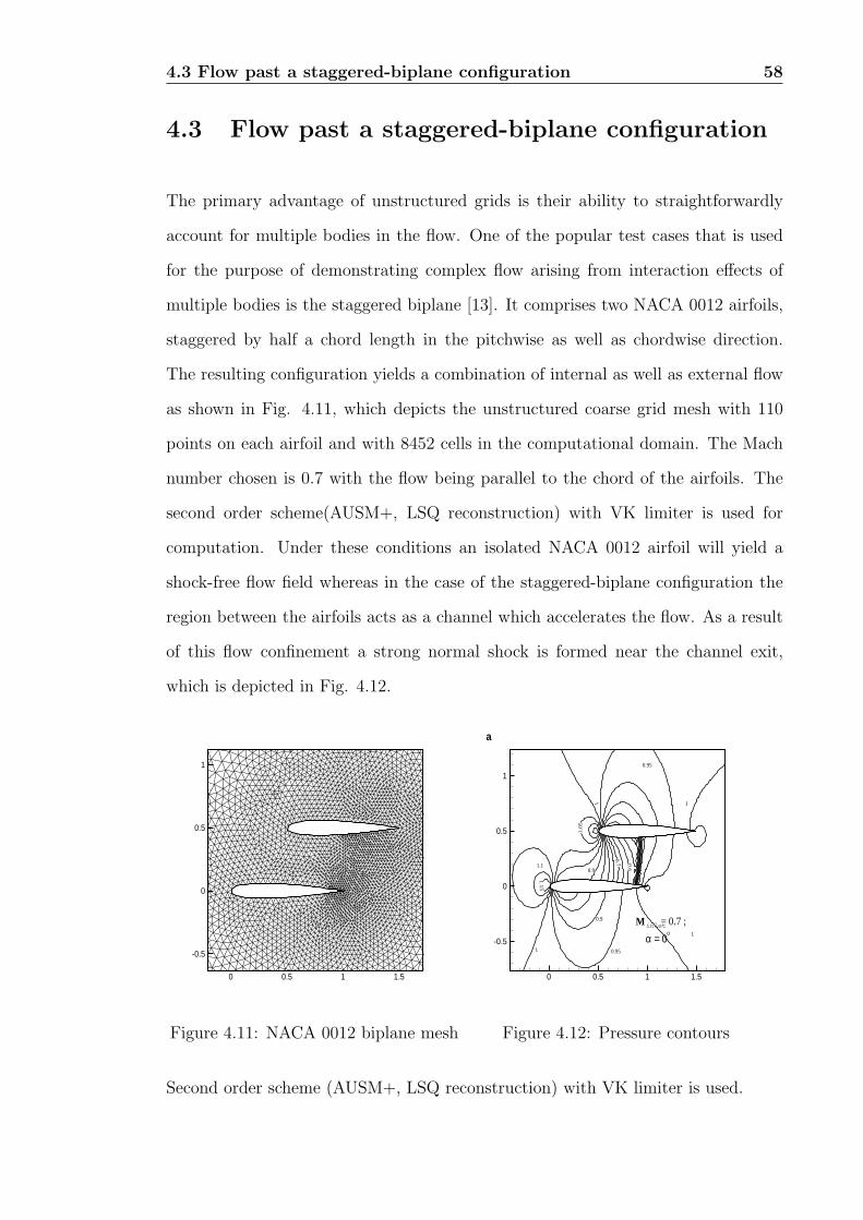
4.3 Flow past a staggered-biplane configuration 58
4.3 Flow past a staggered-biplane configuration
The primary advantage of unstructured grids is their ability to straightforwardly
account for multiple bodies in the flow. One of the popular test cases that is used
for the purpose of demonstrating complex flow arising from interaction effects of
multiple bodies is the staggered biplane [13]. It comprises two NACA 0012 airfoils,
staggered by half a chord length in the pitchwise as well as chordwise direction.
The resulting configuration yields a combination of internal as well as external flow
as shown in Fig. 4.11, which depicts the unstructured coarse grid mesh with 110
points on each airfoil and with 8452 cells in the computational domain. The Mach
number chosen is 0.7 with the flow being parallel to the chord of the airfoils. The
second order scheme(AUSM+, LSQ reconstruction) with VK limiter is used for
computation. Under these conditions an isolated NACA 0012 airfoil will yield a
shock-free flow field whereas in the case of the staggered-biplane configuration the
region between the airfoils acts as a channel which accelerates the flow. As a result
of this flow confinement a strong normal shock is formed near the channel exit,
which is depicted in Fig. 4.12.
0 0.5 1 1.5
-0.5
0
0.5
1
Figure 4.11: NACA 0012 biplane mesh
0.95
0.7 0.6
0.95
0.9
1.1
5
1.1
1.0
5
1 1
1
1
0.9
0 0.5 1 1.5
-0.5
0
0.5
1
Minlet= 0.7 ;
α = 0ο
a
Figure 4.12: Pressure contours
Second order scheme (AUSM+, LSQ reconstruction) with VK limiter is used.

4.3 Flow past a staggered-biplane configuration 59
The accuracy of the solution not only depends on the schemes but also depends on
the resolution of grid pattern. So the coarse grid pattern is refined to 45630 cells.
Figs. 4.13(a) and (b) show the improved solutions after grid refinement. From Figs.
4.13(c) and (d), The computed 3rd order scheme surface pressure distributions are
good agreement with Jawahar and kamath [13] results. Residual history is shown
in Fig. 4.13(e). No convergence difficulty was observed for 2nd case even for a
reduction in the residual up to 9 orders of magnitude.
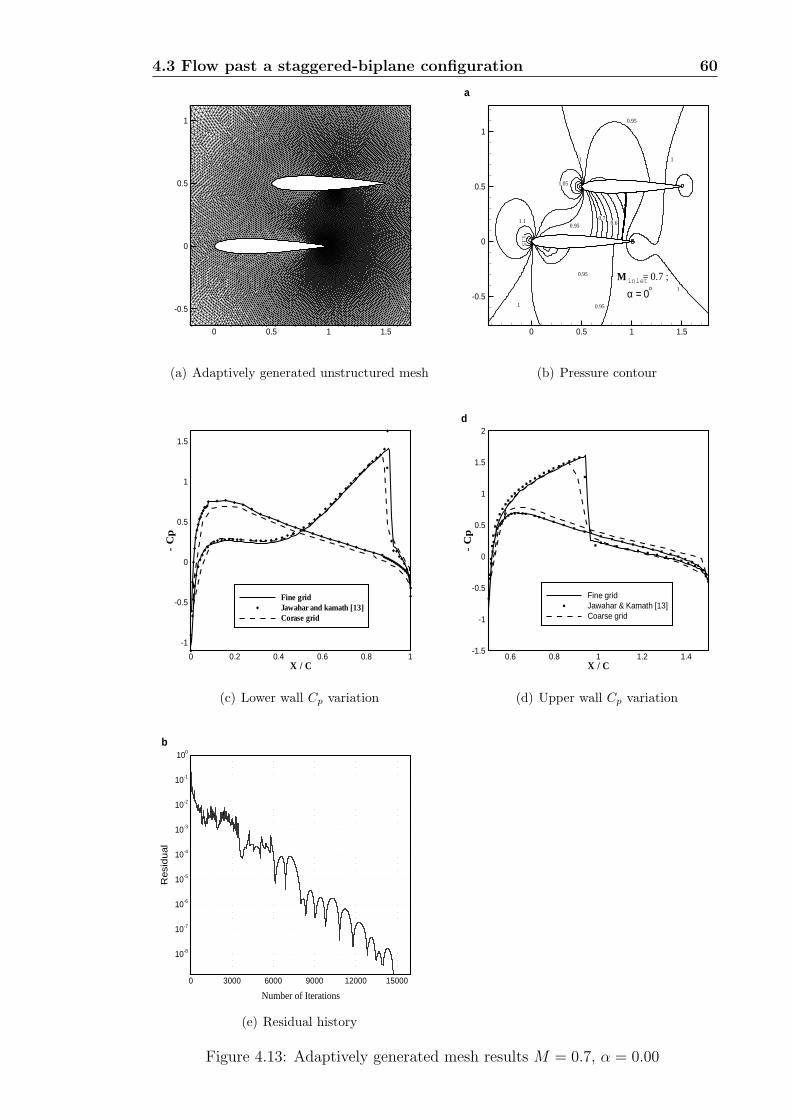
4.3 Flow past a staggered-biplane configuration 60
0 0.5 1 1.5
-0.5
0
0.5
1
(a) Adaptively generated unstructured mesh
0.95
0.70.6
0.95
0.951.15
1.1
1.05
1 1
1
1
0.95
0 0.5 1 1.5
-0.5
0
0.5
1
Minlet= 0.7 ;
α = 0ο
a
(b) Pressure contour
X / C
-C
p
0 0.2 0.4 0.6 0.8 1
-1
-0.5
0
0.5
1
1.5
Fine gridJawahar and kamath [13]Corase grid
(c) Lower wall Cp variation
X / C
-C
p
0.6 0.8 1 1.2 1.4-1.5
-1
-0.5
0
0.5
1
1.5
2
Fine gridJawahar & Kamath [13]Coarse grid
d
(d) Upper wall Cp variation
Number of Iterations
Resi
du
al
0 3000 6000 9000 12000 15000
10-8
10-7
10-6
10-5
10-4
10-3
10-2
10-1
100
b
(e) Residual history
Figure 4.13: Adaptively generated mesh results M = 0.7, α = 0.00
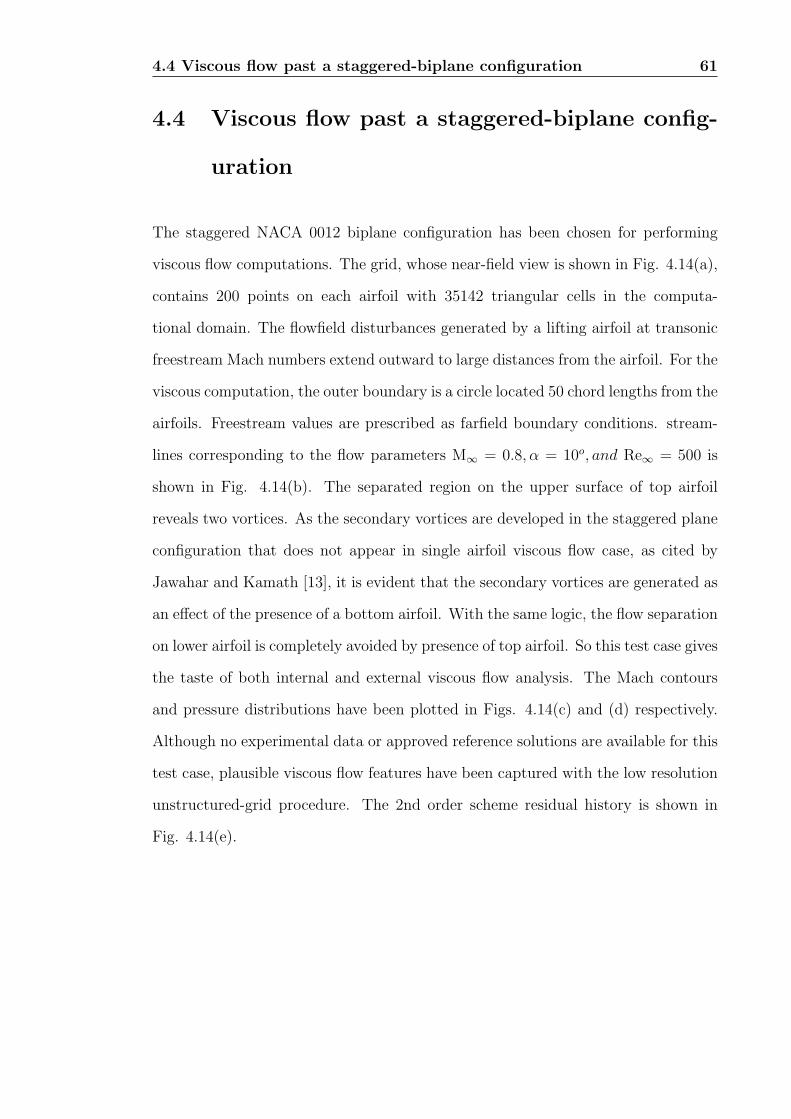
4.4 Viscous flow past a staggered-biplane configuration 61
4.4 Viscous flow past a staggered-biplane config-
uration
The staggered NACA 0012 biplane configuration has been chosen for performing
viscous flow computations. The grid, whose near-field view is shown in Fig. 4.14(a),
contains 200 points on each airfoil with 35142 triangular cells in the computa-
tional domain. The flowfield disturbances generated by a lifting airfoil at transonic
freestream Mach numbers extend outward to large distances from the airfoil. For the
viscous computation, the outer boundary is a circle located 50 chord lengths from the
airfoils. Freestream values are prescribed as farfield boundary conditions. stream-
lines corresponding to the flow parameters M∞ = 0.8, α = 10o, and Re∞ = 500 is
shown in Fig. 4.14(b). The separated region on the upper surface of top airfoil
reveals two vortices. As the secondary vortices are developed in the staggered plane
configuration that does not appear in single airfoil viscous flow case, as cited by
Jawahar and Kamath [13], it is evident that the secondary vortices are generated as
an effect of the presence of a bottom airfoil. With the same logic, the flow separation
on lower airfoil is completely avoided by presence of top airfoil. So this test case gives
the taste of both internal and external viscous flow analysis. The Mach contours
and pressure distributions have been plotted in Figs. 4.14(c) and (d) respectively.
Although no experimental data or approved reference solutions are available for this
test case, plausible viscous flow features have been captured with the low resolution
unstructured-grid procedure. The 2nd order scheme residual history is shown in
Fig. 4.14(e).
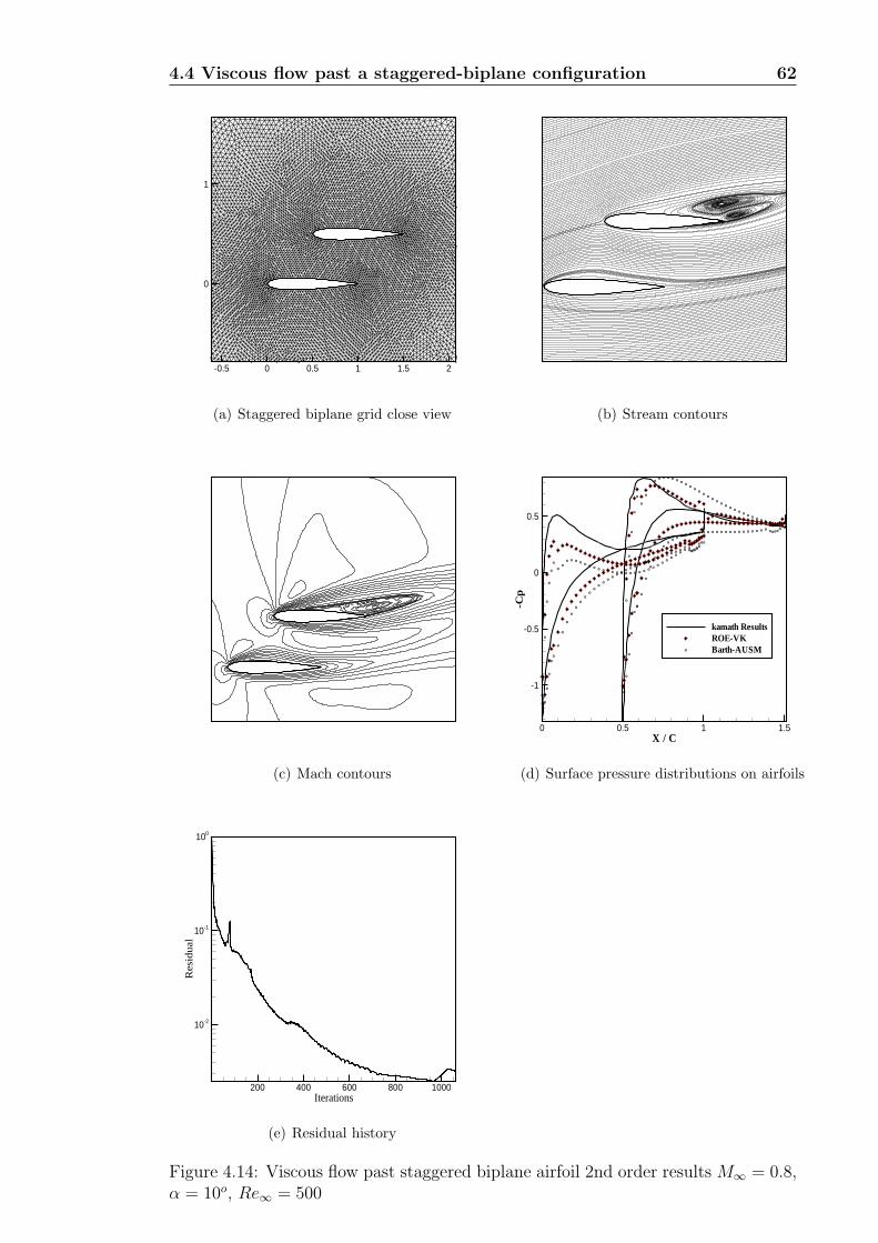
4.4 Viscous flow past a staggered-biplane configuration 62
-0.5 0 0.5 1 1.5 2
0
1
(a) Staggered biplane grid close view (b) Stream contours
(c) Mach contours
oo
o
o
o
oo
o
o
o
o
o
o
oooooooooooo
o
o
oo
o o o o o o o o o o o o o o o o o o o o o o o o o o
ooooooooooooooooooooooo
oo
o
o
o
o
o
o
o
o
o
o
o
o
o
o
o
o
o
ooooooo
ooooo
oo
o o o o o o o o o o o o o o o o o o o o o o oo
oo
o oooooooooooooooooo
oo
oo
oo
oo
o
o
o
o
o
X / C
-Cp
0 0.5 1 1.5
-1
-0.5
0
0.5
kamath ResultsROE-VKBarth-AUSMo
(d) Surface pressure distributions on airfoils
Iterations
Res
idua
l
200 400 600 800 1000
10-2
10-1
100
(e) Residual history
Figure 4.14: Viscous flow past staggered biplane airfoil 2nd order results M∞ = 0.8,α = 10o, Re∞ = 500
Chapter 5
Conclusions and Future Work
The accuracy of the Euler code has been extensively established by comparing with
various test cases. The accuracy of viscous code is ensured and plausible viscous
flow features have been captured with high resolution. Third order scheme is con-
structed and tested for the Euler equations for the arbitrary unstructured meshes.
The properties of various schemes, reconstruction methods and limiters are studied.
Barth limiter faces convergence problems in most of the flow conditions. Venkatakr-
ishnan limiter is comparatively good. But some preliminary work is required in
selection of the parameters to get monotonic and converged solutions. Jawahar and
Kamath limiter also displays good convergence properties. However, it is not very
good at weak shocks compare to the other two limiters.
5.1 Scope for future work
1. The solver can be extended for incompressible computations by employing low
Mach number preconditioning for unstructured schemes.
2. The code can be extended to turbulence computations by adding a suitable

5.1 Scope for future work 64
algebraic turbulent model to it.
3. In order to drastically decrease the computational time, the mode of compu-
tation can be altered to implicit.
Bibliography
[1] Jameson, A. and Mavriplis, D. J. Finite Volume Solution of Two-Dimensional
Euler Equations on Regular Triangular Mesh, AIAA Journal, 24. No. 4,
pp.611-618, April 1986.
[2] Godunov, S.K. A Differnce Scheme for Numerical Computation of Discontin-
uous Solution of Hydrodynamic Equations, Math. Sbornik, 47, pp. 271-306,
1959 (in Russian).
[3] Roe, P. L. Approximate Riemann Solvers, Parameters Vectors and Difference
Schemes. J. Computational Physics, 43, pp.357-372, 1981.
[4] Steger, J. L. and Warming R. F. Flux Vector Splitting of Inviscid Gas-Dynamic
Equations with Application to Finite Differeence Methods, 1981.
[5] van Leer, B., Towards the Ultimate Conservative Difference Schemes Mono-
tonicity and Conservation Combined in Second Order Scheme. J. Computa-
tional Physics, 14, pp.361-370, 1979.
[6] Liou, M. S. and Stefen, C. J. Jr. A New Flux Splitting Scheme, J. Computa-
tional Physics, 107, 1993, pp. 23-39, 1981.
[7] Liou, M. S. A sequel to AUSM: AUSM+, J. Computational Physics, 1993 129,
pp. 364-382, 1981.
BIBLIOGRAPHY 66
[8] Jameson, A. Solutions of the Euler Equations for Two-Dimensional Transonic
Flow by a Multigrid Method. MAE report No.1613, 1983.
[9] Barth T. J. and Dennis C. Jaspersen. The Design and Application of Upwind
Schemes on Unstructured Meshes, AIAA 89-0366, Jan. 1989.
[10] Barth T. J. and Paul O. Frederickson. Higher Order Solution of the Euler
Equations on Unstructured Grids Using Quadratic Reconstruction, AIAA-90-
0013, January 8-11, 1990/Reno, Nevada.
[11] Barth T. J. Recent Developments in High Order K-Exact Reconstruction on
Unstructured Meshes, AIAA-93-0668, January 11-14, 1993/Reno, Nevada.
[12] Delanaye M. and Essers J. A. Quadratic-Reconstruction Finite Volume Scheme
for Compressible Flows on Unstructured Adaptive Grids, AIAA, 35, No. 4,
April 1997.
[13] Jawahar, and Hemanth Kamath P., A High Resolution Procedure for Eu-
ler and Navier-Stokes Computations on Unstructured Grids, J.Computational
Physics, 164, pp. 165-203, 2000.
[14] Liang S, and Chan J., An Improved Upwind Scheme for the Euler Equations,
J.Computational Physics, 84, pp. 461-473, 1989.
[15] Courant, R., Isaacson, E. and Rees, M. On solution of Non-linear Hyperbolic
Differential Equations by Finite Differences, Cpmm.Pure and Applied Mathe-
matics, 5, pp. 243-255, 1952.
[16] Jameson. A. Artificial Diffusion, Upwind Biasing, Limiters and Their Effect
on Accuracy and Multigrid Convergence in Transonic and Hypersonic Flow
AIAA Paper 93-3559, 1982.
[17] Osher, S. and Solomon, F. Upwind Difference Schemes for Hyperbolic System
of Conservation Laws, Math. Comp., 38, pp. 339-374, 1982.
BIBLIOGRAPHY 67
[18] Blazek, J. Computational Fluid Dynamics: Principles and Applications, Else-
vier, 2001.
[19] Venkatakrishnan, V. Prespective on Unstructured Grid Flow Solvers, icase-
1995-3.
[20] Frink, N. T. Upwind Scheme for Solving the Euler Equations on Unstructured
Tetrahedral Meshes, AIAA Journal, 30, No.1, pp.70-77.
[21] Venkatakrishnan, V. Convergence to Steady State Solutions of the Euler Equa-
tions on Unstructured Grids with Limiters, J. Computaional Physics, 118,
120-130,1995.
[22] Rosendale, J. V. Floating shock Fitting via Lagrangian Adaptive Meshes,
ICASE 94-89, 1989.
[23] Jameson, A., Schmidt, W. and E.Turket, Numerical Simulation of the Eu-
ler Equations by Finite Volume Methods Using Runge-Kutta Time Stepping
Schemes, Pres.at the 5th AIAA comput.Flu.Dyn.conf. AIAA-81-1259, 1981.
[24] Charles Hirsh., Numerical Computation of Internal and External Flows, Vol
1 and 2, Wiley, Newyork, 1998.
[25] Bala Krishnan, N. Fernandez, G. Wall Boundary Conditions for Inviscid
Compressible Flows on Unstructured Meshes, Int.J. Numer.Meth.Fluids, 28,
pp.1481-1501, 1998.