Embed Size (px)
Citation preview

NEACRP-L-330
•A
OËCD/NEA Committee on Reacfor Physics (NEACRP)
3-D NEUTRON TRANSPORT BENCHMARKS
Toshikazu TAKEDA and Hideaki IKEDA
Department of Nuclear Engineering
OSAKA UNIVERSITY
Yamada-oka 2-1, Suita, Osaka
Japan
Ma'.ch 1991

NEACRP-L-330
OECD/NEA Committee on Reactor Physics (NEACRP)
3-D NEUTRON TRANSPORT BENCHMARKS
Toshikazu TAKEDA and Hideaki IKEDA
Department of Nuclear Engineering
OSAKA UNIVERSITY
Yamada-oka 2-1 , Suita, Osaka
Japan
March 1991
Abstract
A set of 3-D neutron transport benchmark problems proposed by the Osaka University to
NEACRP in 1988 has been calculated by many participants and the corresponding results are
summarized in this report. The results of keff, control rod worth and region-averaged fluxes for
the four proposed core models, calculated by using various 3-D transport codes arc compared
and discussed. The calculational methods used were: Monte Carlo, Discrete Ordinates (Sn),
Spherical Harmonics (Pn), Nodal Transport and others. The solutions of the four core models
are quite useful as benchmarks for checking the validity of 3-D neutron transport codes.

CONTENTS
page
1 Introduction 1
2 Calculational Benchmark Models 2
2. 1 Model 1 2
2.2 Model 2 2
2.3 Model 3 3
2.4 Model 4 3
3 Convergence and Averaging 3
3. 1 Convergence criteria and flux normalization 3
3.2 Mean values 4
4 Method Description 4
5 Benchmark results 10
5.1 Model 1 11
5.2 Model 2 12
5.3 Model 3 13
5.4 Model 4 14
6 Conclusions 15
Acknowledgement 15
References 15
Appendix 1 : "Specifications of calculational benchmark core models" 85
Appendix 2 : "Reference angular quadrature sets" 91
Appendix 3 : "2-group cross sections and energy group structure for small LWR" 92
Appendix 4 : "4-group cross sections and energy group structure for small FBR
and axially heterogeneous FBR" 93
Appendix 5 : "4-group cross sections and energy group structure for small FBR
with hexagonal-Z geometry" 95
List of Contributions
List of Tables
List of Figures

List of Contributions
participant institute model
2 3 4
Ait Abderrahim,A.
Alcouffe.R.E.
Bryzgalov,V.I.
Buckel.G.
Collins,P.J.
Fletcher,J.K.
Kaise.Y.
Kobayashi,K.
Lee,S.M.
Landeyro,P.A.
Mironovich,Y.N.
Nakagawa.M.
Palmiotti,G.
Rief,H.
Roy.R.
Schaefer,R.W.
Seifert.E.
Takeda.T.
Wagner,M.R.
Wehmann,U.
Yamamoto,T.
Yaroslavzeva,L.N
SCK/CEN
LANL
Kurchatov
KFK
ANL
AEA Technology
MAPI
Kyoto Univ.
Indira Gandhi
ENEA
FEI
JAERI
CEA
CEC-JRC Ispra
EP Montreal
ANL
ZFK
Osaka Univ.
Siemens
INTERATOM
PNC JAPAN
Kurchatov
BELGIUM
U.S.A.
U.S.S.R.
GERMANY
U.S.A.
ENGLAND
JAPAN
JAPAN
INDIA
ITALY
U.S.S.R.
JAPAN
FRANCE
ITALY
CANADA
U.S.A.
GERMANY
JAPAN
GERMANY
GERMANY
JAPAN
U.S.S.R.
• * *
# » •
• • •
# » t
* * • •
* *
* * #
• * «
*
* * * •
# # * #
• * •
• » •
• *
* • •
* • • •
*
* • *
• * • •

List of Tables
Table 1 List of ParticipantsTable 2 List of Codes used for the Benchmark ProblemsTable 3 List of Computer used for the Benchmark ProblemsTable 4 Average keff and control rod worth of Model 1Table 5 Average keff and control rod worth of Model 2Table 6 Average krff and control rod worth of Model 3Table 7 Average keff and control rod worth of Model 4Table 8 Individual results of keff and control rod worth of Model 1 (Monte-carlo method)Table 9 Individual results of keff and control rod worth of Model 1 (Pn method)Table 10 Individual results of kgff and control rod worth of Model 1 (Sn method)Table 11 Individual results of keff and control rod worth of Model 1 (Other methods)Table 12 Individual results of keff and control rod worth of Model 2 (Monte-carlo method)Table 13 Individual results of keff and control rod worth of Model 2 (Pn method)Table 14 Individual results of k£ff and control rod worth of Model 2 (Sn method)Table 15 Individual results of keff and control rod worth of Model 2 (Other methods)Table 16 Individual results of keff and control rod worth of Model 3 (Monte-carlo method)Table 17 Individual results of keff and control rod worth of Model 3 (Pn method)Table 18 Individual results of keff and control rod worth of Model 3 (Sn method)Table 19 Individual results of keff and control rod worth of Model 3 (Other methods)Table 20 Individual results of keff and control rod worth of Model 4 (Monte-carlo method)Table 21 Individual results of keff and control rod worth of Model 4 (Pn method)Table 22 Individual results of keff and control rod worth of Model 4 (Sn method)Table 23 Individual results of keff and control rod worth of Model 4 (Other methods)Table 24 Region-averaged fluxes of Model 1, case 1 (Method-averaged values)Table 25 Region-averaged fluxes of Model 1, case 2 (Method-averaged values)Table 26 Region-averaged fluxes of Model 2, case 1 (Method-averaged values)Table 27 Region-averaged fluxes of Model 2, case 2 (Method-averaged values)Table 28 Region-averaged fluxes of Model 3, case 1 (Method-averaged values)Table 29 Region-averaged fluxes of Model 3, case 2 (Method-averaged values)Table 30 Region-averaged fluxes of Model 3, case 3 (Method-averaged values)Table 31 Region-averaged fluxes of Model 3, case 3 (Method-averaged values)Table 32 Region-averaged fluxes of Model 3, case 3 (Method-averaged values)Table 33 Region-averaged fluxes of Model 3, case 3 (Method-averaged values)Table 34 Individual results of region-averaged fluxes of Model 1, case 1 (Monte-Carlo method)Table 35 Individual results of region-averaged fluxes of Model 1, case 1 (Pn method)Table 36 Individual results of region-averaged fluxes of Model 1, case 1 (Sn method)Table 37 Individual results of region-averaged fluxes of Model 1, case 1 (Other methods)Table 38 Individual results of region-averaged fluxes of Model 1, case 2 (Monte-Carlo method)Table 39 Individual results of region-averaged fluxes of Model 1, case 2 (Pn method)Table 40 Individual results of region-averaged fluxes of Model 1, case 2 (Sn method)Table 41 Individual results of region-averaged fluxes of Model 1, case 2 (Other methods)Table 42 Individual results of region-averaged fluxes of Model 2, case 1 (Monte-Carlo method)Table 43 Individual results of region-averaged fluxes of Model 2, case 1 (Pn method)

List of Tables (contd)
Table 44 Individual results of regionTable 45 Individual results of regionTable 46 Individual results of regionTable 47 Individual results of regionTable 48 Individual results of regionTable 49 Individual results of regionTable 50 Individual results of regionTable 51 Individual results of regionTable 52 Individual results of regionTable 53 Individual results of regionTable 54 Individual results of regionTable 55 Individual results of regionTable 56 Individual results of regionTable 57 Individual results of region-Table 58 Individual results of regionTable 59 Individual results of region-Table 60 Individual results of region-Table 61 Individual results of region-Table 62 Individual results of region-Table 63 Individual results of region-Table 64 Individual results of region-Table 65 Individual results of region-Table 66 Individual results of region-Table 67 Individual results of region-Table 68 Individual results of region-Table 69 Individual results of region-Table 70 Individual results of region-Table 71 Individual results of region-Table 72 Individual results of region-Table 73 Individual results of region-
-avcraged fluxes of Model 2, case-averaged fluxes of Model 2, case-averaged fluxes of Model 2. case-averaged fluxes of Model 2, case-averaged fluxes of Model 2, case-averaged fluxes of Model 2, case-averaged fluxes of Model 3, case-averaged fluxes of Model 3, case-averaged fluxes of Model 3, case-averaged fluxes of Model 3, case-averaged fluxes of Model 3, case-averaged fluxes of Model 3, case-averaged fluxes of Model 3, case-averaged fluxes of Mode! 3, case-averaged fluxes of Model 3, case-averaged fluxes of Model 3, case-averaged fluxes of Model 3, case-averaged fluxes of Model 3, case•averaged fluxes of Model 4, case-averaged fluxes of Model 4, case•averaged fluxes of Model 4, case•averaged fluxes of Model 4, case-averaged fluxes of Model 4, case•averaged fluxes of Model 4, case•averaged fluxes of Model 4, case•averaged fluxes of Model 4, case•averaged fluxes of Model 4, caseaveraged fluxes of Model 4, caseaveraged fluxes of Model 4, caseaveraged fluxes of Model 4, case
1 (Sn method)1 (Other methods)2 (Monte-Carlo method)2 (Pn method)2 (Sn method)2 (Other methods)1 (Monte-Carlo method)1 (Pn method)1 (Sn method)1 (Other methods)2 (Monte-Carlo method)2 (Pn method)2 (Sn method)2 (Other methods)3 (Monte-Carlo method)3 (Pn method)3 (Sn method)3 (Other methods)1 (Monte-Carlo method)1 (Pn method)1 (Sn method)1 (Other methods)1 (Monte-Carlo method)1 (Pn method)1 (Sn method)1 (Other methods)1 (Monte-Carlo method)1 (Pn method)1 (Sn method)1 (Other methods)
List of Figures
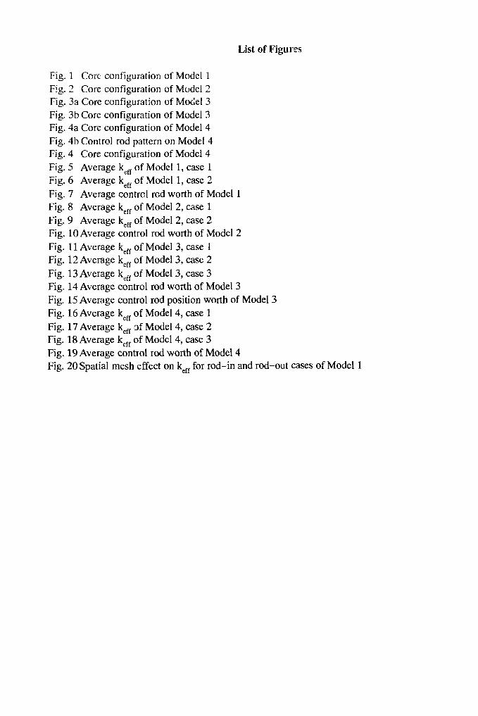
Fig. 1 Core configuration of Model 1Fig. 2 Core configuration of Model 2Fig. 3a Core configuration of Model 3Fig. 3b Core configuration of Model 3Fig. 4a Core configuration of Model 4Fig. 4b Control rod pattern on Model 4Fig. 4 Core configuration of Model 4Fig. 5 Average ke£f of Model 1, case 1Fig. 6 Average keff of Model 1, case 2Fig. 7 Average control rod worth of Model 1Fig. 8 Average keff of Model 2, case 1Fig. 9 Average keff of Model 2, case 2Fig. 10 Average control rod worth of Model 2Fig. 11 Average keff of Model 3, case 1Fig. 12 Average keff of Model 3, case 2Fig. 13 Average keff of Model 3, case 3Fig. 14 Average control rod worth of Model 3Fig. 15 Average control rod position worth of Model 3Fig. 16 Average kgff of Model 4, case 1Fig. 17 Average keff of Model 4, case 2Fig. 18 Average keff of Model 4, case 3Fig. 19 Average control rod worth of Model 4Fig. 20 Spatial mesh effect on keff for rod-in and rod-out cases of Model 1

1. Introduction
This is the final report on the results of the "3-D Neutron Transport Benchmark Prob-
lems" proposed from Osaka University to NEACRP in 1988(1). The purpose of this benchmark
proposal was to compare the results of each participant to investigate the accuracy of individual
methods, and to set up 3-D neutron transport benchmarks to be used in the future to check the
validity of 3-D neutron transport codes.
In this benchmark problem, four models were proposed and twenty two members (twenty
organizations) participated.
To discuss the results a working group meeting was held on October 22 and 23, 1990 in
Saclay with the sponsorship of OECD-NEA.
At the meeting the method of summarizing the results was discussed and determined in
addition to the comparison of the individual calculational results.
It was decided to obtain mean values and standard deviations of keff, control rod worth,
and region-averaged group fluxes for each calculation method; mean values are taken separately
for the results obtained in the Sn, Monte-Carlo method, etc. Further, there was a unified opinion
about the averaging for the Monte-Carlo method: the inverse of variance should be used as a
weight to obtain the mean value.
Also through comparison some errors in calculational results were found, and it was
recommended to include the updated results in this final report.
Four calculational benchmark models are illustrated in Chap. 2. In Chap. 3 the conver-
gence criterion and the flux normalization are described.
In Chap. 4 the methods utilized by individual participants are described.
The mean values and standard deviations of keff, control rod worth and region-averaged
-1-

group fluxes are shown in Chap. 5.
For the mean value we used the latest contribution from each participant. When a result
deviated greatly from other results we excluded it from averaging.
2. Calculational Benchmark Models
The full problem specification of the proposed benchmark cores was described in the
NEACRP report A-953 Rev. 1(1), and it is included in Appendix 1 of this report. The simple
explanation of the proposed cores is described below.
2.1. Model 1 (Small LWR)
This core is a model of the Kyoto University Critical Assembly (KUCA). The core
configuration is shown in Fig. 1. The reference mesh size is lem x lem x lcm.
The core calculation is performed in 2 groups. The 2-group cross section set and energy
group structure are given in Appendix 3.
We considered the following two cases;
case 1 : the control rod position is empty (void)
case 2 : the control rod is inserted
2.2. Model 2 (Small FBR)
The core geometry (quarter core) is shown in Fig. 2, and the reference mesh size is 5cm
x 5cm x 5cm. These two cases are considered:
case 1 : the control rod is withdrawn (the control rod position is filled with Na)
case 2 : the control rod is half-inserted
The core calculation is performed in 4-groups. The 4-group cross sections and energy
-2-

group structure arc listed in Appendix 4.
2. 3. Model 3 (Axially heterogeneous FBR)
This core has an internal blanket region as shown in Fig. 3 (1/8 geometry). In this model,
5cm x 5cm x 5cm mesh interval in the 1/8 core model is the reference mesh size. The 4-group
cross sections and energy group structure which are used for calculations are given in Appendix
4.
We consider the following three cases :
case 1 : the control rods are inserted
case 2 : the control rods are withdrawn
case 3 : the control rods are replaced with core and/or blanket cells
2. 4. Model 4 (Small FBR with Hexagonal-Z geometry)
This core model is proposed by I. Breeders and E. Kiefhaber of KFK, Germany, and is a
model of the KNK-II core(2). This model has a Hexagonal-Z geometry as shown in Fig. 4.
Energy group structure and cross sections in four groups are listed in Appendix 5.
The control rod patterns are considered as follows:
case 1 : the control rods are withdrawn
case 2 : the control rods are half-inserted
case 3 : the control rods are fully-inserted
3. Convergence and Averaging
3.1 . Convergence criteria and flux normalization
The suggested convergence criteria were
-3-

5x 1(T4
Akeff/keff < 5xlO"5.
Some participants used smaller values.
The normalization of fluxes is
2 / v d r v2 [ g(r)$g(r) =[g(
3. 2 Mean values
The average method used for Monte-Carlo results are as below,
x.. 1x = Z — / Z -
i of i of
1 1y
a2
where x = mean value
Xj = individual Monte-Carlo results
of = variance of individual result x.
a2 = variance of the mean.
The averages of all Monte-Carlo results are calculated. However, to obtain reference solutions
the averages of Monte-Carlo results excluding results calculated with perturbation Monte-Carlo
codes, and results which are obviously different from the reference solutions are calculated.
The conventional mean values and standard deviations are used for the other methods
since they do not have uncertainly estimates.
4. Method Description
-4 -

We describe the methods used by participants briefly.
VIM code™
The Monte-Carlo code "VIM" calculations are one of the codes used at ANL (Schaefcr
and Fanning) for the benchmark calculation. Usually, the VIM calculatios arc performed with
continuous energy, and it uses ENDF/B cross section data. However, it was modified to use the
given set of multigroup cross sections. No variance reduction techniques were used. A batch
size of 10,000 histories was used and 250 batches were run for each case.
KENEUR code14*
The Monte-Carlo code "KENEUR" was used by Rief for the benchmark problem. This
code is a modified version of the KENO-IV. Perturbation estimates of the eigenvalues, flux
estimates, reaction rates and power distributions are based on the Green's function (fission ma-
trix) approach, in which the fissionable region is subdivided into a mesh of appropriately chosen
volume elements. To allow for more flexibility in the subdividion of the fissionable space of a
multiplying system apart from "Units" and "Boxes" which are the volume elements provided by
KENO-IV in KENEUR, all geometrical regions can become volume elements.
During the benchmark exercise two modifications were made which improved considera-
bly the originally submitted results: 1) To make the requirement of "appropriately chosen"
volume elements less stringent, a method to approximate the perturbed source distribution in
each volume element was developed and 2) the single precision flux and reaction rate arithmetic
of KENO-IV had been changed to the double precision.
MCUcode^
Bryzgalov calculated Models 1, 2 and 4 with the Monte-Carlo code "MCU". Number of
histories per generation is 200, and the total histories are approximately 500,000.
-5-

KENO-IVcode^
Landeyro estimated Models 1, 2 and 3 with the Monte-Carlo code "KENO-IV". All
calculations were performed with 480 batches of 1,000 neutrons.
GIWP codé»
The Monte-Carlo code "GMVP" was used by Nakagawa for all the benchmark problems.
Number of histories for Model 1 is 2 million, and 1 million for Models 2, 3 and 4.
MOCA code™
Wehmanii estimated Models 2, 3 and 4 with the Monte-Carlo code "MOCA". Each case
was ca. _iated by the history of 150 neutrons during 12,000 generations, thus by 1.8 million
histories.
OMEGA code™
Seifert used the perturbation Monte-Carlo code "OMEGA" and calculated Models 1, 2
and 4. Number of histories is 200,000 for Model 1, and 150,000 for Model 2 and 4.
TRITAC code™
The TRITAC which uses the discrete ordinates method was developed at Osaka Universi-
ty. This code is based on the three-dimensional diffusion synthetic acceleration method.
Buckel, Lee, Yamamoto, and Takeda used the TRITAC code for this benchmark prob-
lem.
Takeda calculated with reference mesh intervals and half mesh intervals for Models 1 and
2, and calculated with the order S4 and Sg for all models.
Yamamoto calculated Models 2 and 3 with S4 and Sg discrete ordinates.
Buckel calculated Models 1, 2 and 3 with S4, Sg and S16 discrete ordinates.
Lee calculated Models 1, 2 and 3 with S4 and Sg discrete ordinates.

THREEDANT code{U)
THREEDANT is the three-dimensional neutron transport calculation code using the
discrete ordinates method and based on the ONEDANT-TWODANT system. In this code the
three-dimensional DSA method is adopted for the acceleration, further the DSA equation is
accelerated by Chebychev technique and is inverted using a three-dimensional multigrid tech-
nique.
Alcouffe used this code for the benchmark calculation, and he calculated with reference
mesh intervals for S4, Sg, S12 and S16 solutions and with half mesh intervals for S8 solution.
JAR-SN code™
This code is for solving multigroup two- or three-dimensional transport equation with
rectangular or hexagonal space meshes. The calculations are carried out for a whole reactor and
symmetry angle 60° (for hexagonal geometry).
Yaloslavzeva used this code and calculated S2, S4 and Sg solutions with reference mesh
intervals.
ENSEMBLE-K code™
This Sn code was used by Kaise to calculated Models 1 and 2. S4 solutions were given
for each case.
MARK-
Fletcher calculated the benchmark problem with the MARK-PN code which employs an
expansion of the flux in spherical harmonics. Eigenvalues are quoted for Pj to P7 and other re-
sults are taken from the P7 case.
Fletcher also calculated with half mesh intervals and estimated the zero mesh keff by
extrapolation. He calculated Model 4 with the triangular-Z geometry.
-7-

PLXYZcode^
Kobayashi calculated Model 1 with the PLXYZ code, and he gave Pj, P3 and P5 results.
Further, he estimated îhe Pinfinit eigenvalue by extrapolation. He calculated with a fine mesh
(30cmx30cmx30cm).
DIF3D code(16)
Collins (ANL) used the nodal transport theory (NTT) and nodal diffusion theory (NDT)
method, as implemented in the DIF3D code, to calculate Models 2 and 3.
The polynomial approximation to the flux direction of solution was quaratic for NTT and
cubic for NDT. The quadratic polynomial approximation to the transverse leakage was made.
Coarse mesh rebalancing with asymptotic source extrapolation was used to accelerate the outer
iterations. The eigenvalue convergence criteria was l.OxlO"7, and the convergence criteria for
average fission source and pointwise fission source was l.OxlO"5.
The node sizes are as below:
Model 2 : 14x5cm in X, 14.5x5cm in Y, 7xl0cm, 2x5cm and 7xl0cm in Z
Model 3 : 32x5cm in X, 32x5cm in Y, 2x5cm, 4xl0cm, Ix5cm, 2xl2.5cm and lxlOcm
in Z
HEXNOD
Wagner calculated Model 4 with the HEXNOD code which uses the nodal transport (NT)
or nodal diffusion (ND) theory.
Regular meshes of hexagonal are prismatic nodes. Partial interface current method with
boundary fluxes and currents in PI and DPI approximations are used in the HEXNOD code.
Group response matrix equations are solved during the global outer iteration process. Conver-
gence is accelerated by coarse mesh rebalancing and asymptotic fission source extrapolation.
Wagner calculated with 12 or 20 axial layers.

Combination method (CCRR code)m)
Palmiotti used the CCRR code, which is a the combination method of 3-D diffusion and
2-D transport.
The 3-D transport effect is estimated by R-Z transport calculation, R-Z diffusion calcu-
lation and 3-D diffusion calculation by
K, DIF
TR _ v TR ,. ^n - "-R7 x
KRZ
The diffusion values are extrapolated to zero mesh.
Synthesis method (DOT3.5 code)(ï9)
Synthesis method and DOT3.5 code are used by Ait Abderrahim.
Synthesis method is a combination of 2-D transport theory and 1-D transport theory, and
a 3- D synthesized flux <E>(x,y,z) is obtained by weighting the plane flux map O(x,y) by axial
function f(z):
<E>(x,y,z) = 0>(x,y) x f(z)
This f(z) is derived by using 2-D transport (r,z), (x,z) or (y,z) calculations and 1-D
transport (r), (x) or (y) calculations.
f(z) =
<D(r)
O(x,z)
depending on the model considered.
-9 -

CMEZ code™
Mironovich used this code to calculate Model 4. This code uses the combination method
of 3-D diffusion and 2-D (R-Z and triangular) and 1-D (cylinder) transport correction, which is
indicated as follows:
K" TO _ f̂ DIF , (V TR 17 DIF\ , fv TR_i/- DIF\ , (v TR ^ DI1\
3-D collision probability transport code "DMGON"(2l)
Roy used this code to calculate the benchmark problems, and this code can treat, in addi-
tion to purely Cartesian geometries, mixed cylindrical-Cartesian region, for example, a finite
cylinder inserted inside a cube.
Extrapolated values in Pn and Sn method
In Pn and Sn methods, zero mesh keff is obtained by the following extrapolation.
Ak = k(zero mesh interval) - k(Nx,Ny,Nz)
= A/Nx 2 + B/Ny2 + C/Nz2
where Nx, Ny and Nz are number of the mesh on each axis.
Also S.nfinit values are estimated by
= D / n s E /N 2
where N is the number of discrete ordinates directions.
5. Benchmark results
Mean values and standard deviations of kcff and control rod worth are listed in Tables 4 to
7 for each method and for each model. The same results are shown in Figs. 5 to 19.
-10-

All results of keff and control rod worth contributed from all participants arc listed in
Tables 8 to 23.
Average values of region-averaged group fluxes are listed in Tables 24 to 33.
The region-averaged fluxes from all participants are listed in Tables 34 to 73.
Fig. 20 shows the spatial mesh effect on keff for rod-in and rod-out cases of Model 1.
5. 1. Model 1: Small LWR Core
Table 4 lists the mean values and standard deviations of keff and control rod worth, and
Tables 24 and 25 gives the region-averaged fluxes. In the Monte-Carlo method the standard
deviation of keff is ~0.0005Ak, and the relative standard deviation of control rod worth is about
4%. The standard deviations of the region-averaged fluxes are very small.
In the case of the Sn method, keff and the control rod worth scatter very little compared
with those in the Monte-Carlo method. It should be mentioned, however, that the angular
quadrature effect and the spatial mesh effect are relatively large. kcff by S^ calculation differs
from that by Sg calculation by 0.0006Ak in the rod-out case and 0.0002Ak in the rod-in case. In
the rod-out case, a void region is present at the control rod position, and this makes the angular
quadrature effect significant. The spatial mesh effect on keff is shown in Fig. 20 as a function of
the square inverse of the mesh interval. It is seen that the spatial mesh effect is relatively large in
the rod-in case; this is opposite to the angular quadrature effect. The reason for this is that a fine
mesh calculation is necessary to treat the flux depression adequately around the control rod. The
S8 results in Table 4 have been corrected for the mesh effect, and are in close agreement with the
Monte-Carlo results. The differences in keff and in the control rod worth are within. 1.5a, where
a is the exact Monte-Carlo standard deviation. Nakagawa used two million histories for each
calculation in Model 1, and his Monte-Carlo results are more close to the S8 results, (see Table
8) The region-averaged fluxes are also close to the Monte-Carlo results, difference being
within 1% in all regions and in all energy groups.
In the Pn method, the standard deviations are rather large. Fletcher evaluated the mesh
-11-

effect by calculating kcff with normal mesh interval of 1.0 cm and with half mesh interval of 0.5
cm, and by extrapolating to the zero mesh interval. His kcff values in the P7 calculation are
0.9772 for case 1 and 0.9638 for case 2, giving the control rod worth of 1.42xlO~2. The spatial
mesh effect on keff is large, i. e., 0.0044Ak in case I, and 0.0024Ak in case 2. Even after the
correction, however, the difference from the Monte-Carlo results remains large, particularly for
keff for the rod-in cases. The standard deviation of region-averaged fluxes shown in Tables 24
and 25 is rather large especially in the thermal group in the reflector regions. The difference of
the thermal fluxes from the Monte-Carlo results is large; about 8% in the void region. The same
tendency is seen also for the rod-in case.
5. 2. Model 2: Small FBR Core
Table 5 lists the mean values and standard deviations of kcff and control rod worth, and
Tables 26 and 27 lists the region-averaged fluxes.
The standard deviation of Monte-Carlo keff are about half those of Model 1. The small
standard deviation is due to the fact that the thermal neutron flux is small compared to that in
Model 1 and there is no need to follow neutron histories down to thermal low energy range. For
the region-averaged fluxes the standard deviation is very small except for the 4th group flux; the
maximum standard deviation of the flux is seen at the sodium filled control rod position region
of about 1.5%.
For Sn methods, a good agreement is observed for keff between the S4 and S8 calculations
and the angular quadrature effect is smaller than that in Model 1 because of the nearly isotopic
angular flux distributions in fast reactors. The spatial mesh effect was investigated by Alcouffe,
Yamamoto, and Takeda. The difference between Sg calculations with 5cm x 5cm x 5cm mesh
intervals and 2.5cm x 2.5cm x 2.5cm mesh intervals is rather small, though the difference is a
little dependent on the codes utilized. For example, Alcouffe reported the difference is -0.0001,
and -0.0002Ak for cases 1 and 2, respectively. The agreement of keff and control rod worth with
the exact Monte-Carlo results is very good. The keff difference is less than 0.0003Ak. The
- 1 2 -

region-averaged group fluxes also agree well with the Monte-Carlo results.
For the P7 method the keff difference from the Monte-Carlo results is ~0.0()6Ak for both
cases, and the control rod worth relative difference is - 3 % . These results are the mesh corrected
ones. The core flux is about 2% smaller and the blanket flux is 5% larger in the first group.
Collins calculated with the nodal transport method, and the difference of keff from the
Monte-Carlo is about 0.002Ak.
5. 3. Model 3: Axially Heterogeneous FBR Core
Table 6 lists the mean values and standard deviations of keff and the control rod worth,
and Tables 28, 29 and 30 the region-averaged fluxes. The control rod worth is the change in
l/keff from case 1 to case 2 and the control rod position worth is the change in l/keff from case 2
to case 3.
For the Monte-Carlo results the standard deviation of keff is small and close to the results
of Model 2. For the region-averaged fluxes, the standard deviation is largest in the 4th energy
group but is always less than 1% for the for the Monte-Carlo average.
For the Sn method, the tendencies of the angular quadrature sensitivity in cases 1, 2 and 3
are the same, i. e., the S4 and Sg ke£f difference is about 0.0006Ak for all cases. The Sg calcula-
tion is in good agreement with the Monte-Carlo calculation for cases 2 and 3; for case 1 the S4
keff is even closer to the Monte-Carlo one than the Sg keff. But for TRITAC solutions calculated
by Buckel, Yamamoto, and Takeda, Sg average keff results were 0.9708, 1.0007 and 1.0214 for
cases 1, 2, 3 and 3.08E-02 for control rod worth, respectively, and these values are rather close
to the Monte-Carlo results. Furthermore, Monte-Carlo averages obtained from Wehmann's and
Schaefer's results were 0.9707, 1.0005, 1.0214 and 3.08E-02 for cases 1, 2, 3 keff and control rod
worth, respectively, and these results are in good agreement with the TRITAC solutions des-
crived above. The fluxes in the core, blanket, and control rod position regions agree with the
Monte-Carlo results within 1%. The flux discrepancy in the control rod is between 1%~2%.
For the Pn results, the keff and control rod worth differences from the Monte-Carlo ones
-13-

are large even in the P7 calculation; especially the control rod worth is relatively underestimated
by 10%. However, P3 (half mesh interval (2.5cm)) solutions are rather close to the Monte-Carlo
ones; the relative control rod worth difference is -3.3%, and this fact indicates that the fine mesh
calculation is very important in the Pn method.
The nodal transport keff are slightly underestimated, however, the control rod worth is in
good agreement with the Sg calculation.
5. 4. Model 4: Small FBR Core with Hexagonal~Z Geometry
Table 7 lists the mean values and standard deviations of kcff and control rod worth, and
Tables 31, 32 and 33 the region-averaged fluxes.
The standard deviation of keff and control rod worth for the Monte-Carlo method is
smaller than other methods, and slightly larger than that of Models 2 and 3.
For the Sn method keff and control rod differences from the Monte-Carlo method are
large, and the standard deviations of the Sn results are large especially for the.control rod worth.
The accuracy of the Sn method in this hexagonal-Z geometry model is not good compared to the
XYZ geometry, this is because the flux varies rapidly with positions in the hexagonal plane,
making one mesh per hexagon too coarse to be accurate. One of improvements is to use a trian-
gular-Z geometry Sn code so that the spatial truncation error can be reduced.
The Pn results are close to the Monte-Carlo results, and the control rod worth difference
is ~ 1 % . Fletcher calculated this model with the triangular-Z geometry, and estimated the spatial
mesh effect by calculating with half mesh intervals. The keff results of the P7 calculation with
3.75cm mesh intervals are similar to the Monte-Carlo results, while the 7.5cm mesh P7 results
are larger than the half-mesh results by 0.002, 0.008, and 0.016Ak for cases 1, 2, and 3, respec-
tively.
Wagner calculated keff and control rod worth with the HEXNOD code, which is the nodal
transport code for the hexagonal-Z geometry. His results are close to the Monte-Carlo ones,
especially for the control rod worth.
- 1 4 -

For hcxagonal-Z geometry, the Sn method can suffer from large spatial truncation errors.
In the contrast, the nodal transport method has sufficient spatial accuracy.
6. Conclusions
The four models were calculated by Monte-Carlo method, Sn method, Pn method, nodal
transport theory and other methods. The exact Monte-Carlo solutions, which were obtained from
Monte-Carlo results excluding the perturbation Monte-Carlo ones and results with large errors,
were used as reference solutions.
For XYZ geometry (Models 1, 2 and 3), a good agreement was seen between the calcula-
tional results by the Monte-Carlo method and the Sn method for keff, control rod worth and
region-averaged group fluxes. For the Pn method a rather large discrepancy from the Monte-
Carlo solutions was seen. For hexagonal-Z geometry (Model 4), the Sn method was not accu-
rate. The Pn and the nodal transport methods produced results which were in good agreement
with Monte-Carlo method.
We have established the 3-D neutron transport benchmarks, and this benchmark report
will be useful for the development of 3-D neutron transport calculation codes in the future.
Acknowledgement
In summarizing the results we got kind comment from many participants. Furthermore,
we asked many participants for a large number of numerical results, and they kindly agreed to
send us the results in spite of the laborious work. We want to express our great appreciation for
this kind cooperation, and want to note this report is cooperative effort of all participants.
-15-

Furthermore, we want to express our appreciation to Dr. Sartori for the kind arrangement
of the working group and for the nice suggestion for summarizing this report.
References
(1): Takeda, T., Tamitani, M. and Unesaki, H. "Proposal of 3-D Neutron Transport Benchmark
Problems" NEACRP A-953 REV. 1, October 1988
(2): Kiefhaber, E., Private Communication, 1988
(3): Blomquist, R. N. et al., "VIM - A Continuous Energy Monte-Carlo Code atANL", A Re-
view of the Theory and Application of Monte-Carlo Methods Proc. of a Seminar Workshop,
Oak Ridge, TN, April 21-23, 1980
(4): Rief, H., "KENEUR-A Monte-Carlo Program for Perturbation Analysis In A Multiplying
System", Proc. International Reactor Physics Conference, Jackson Hole, Wyoming, USA, Sep-
tember 18-22, 1988
(5): Maiorov, L. N. Yudkevich, M. S., Vopr. Atom. Nauk. i Techn.(Fiz. i Techn. Nucl. React.)
N7 1985, p.54
(6): Pétrie, L. and Cross, N., "KENO-IVAn Improved Monte-Carlo Criticality Program",
ORNL-4938, 1975
(7): Nakagawa, M., Mori, T., Sasaki, M., "Development of Monte-Carlo Code for Particle
Transport Calculations on Vector Processors", Proc. of International Conference on Supercom-
puting in Nuclear Applications, Mito, Japan, March 12-16, 1990
(8): Lieberoth, J., "A Monte-Carlo Technique to Solve the Static Eigenvalue Problem of the
Boltzmann Transport Equation", Nukleonik 11, 213-219, 1968
(9): Seifert, E., "The Monte-Carlo Criticality Code OMEGA", ZfK-report 364, 1978
(10): Bando, N., Yamamoto, T., Saito, Y. and Takeda, T., "Three-Dimensional Transport
Calculation Method for Eigenvalue Problems Using Diffusion Synthetic Acceleration", J. Nucl.
-16-
Sci. Tech., October 1985
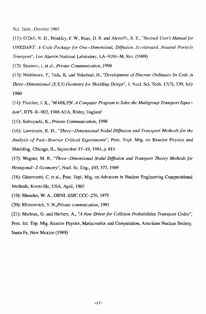
(11): O'Dell, R. D., Brink ley, F. W., Marr, D. R. and Alcouffe, R. E., "Revised User's Manual for
ONEDANT: A Code Package for One-Dimensioal, Diffusion Accelerated, Neutral Particle
Transport", Los Alamos National Laboratory, LA-9184-M, Rev. (1989)
(12): Slesarev, I. et al., Private Communication, 1990
(13): Nishimura, T., Tada, K. and Yokobori, H., "Development of Discrete Ordinales Sn Code In
Three-Dimensional (X,Y,Z) Geometry for Shielding Design", J. Nucl. Sci. Tech. 17(7), 539, July
1980
(14): Fletcher, J. K., "M4RK/PN .A Computer Program to Solve the Multigroup Transport Equa-
tion", RTS-R-002, 1988 AEA, Risley, England
(15): Kobayashi, K., Private Communication, 1990
(16): Lawrence, R. D., "Three-Dimensional Nodal Diffusion and Transport Methods for the
Analysis of Fast-Reactor Critical Experiments", Proc. Topi. Mtg. on Reactor Physics and
Shielding, Chicago, IL, September 17-19, 1984, p. 814
(17): Wagner, M. R., "Three-Dimensional Nodal Diffusion and Transport Theory Methods for
Hexagonal-Z Geometry", Nucl. Sc. Eng., 103, 377,1989
(18): Giacometti, C. et al., Proc. Topi. Mtg. on Advances in Nuclear Engineering Computational
Methods, Knoxville, USA, April, 1985
(19): Rhoades, W. A., ORNL RSIC CCC-276,1975
(20): Mironovich, Y. N.frivate commnication, 1991
(21): Marleau, G. and Herbert, A., "A New Driver for Collision Probabilities Transport Codes",
Proc. Int. Top. Mtg. Reactor Physics, Mathematics and Computation, American Nuclear Society,
Santa Fe, New Mexico (1989)
- 1 7 -

Table 1 List of participants
Model 1
participant institute method
P.A.Landeyro
H.Rief
E.Seifert
V.I.Bryzgalov
M.Nakagawa
G.Palmiotti
J.K.Fletcher
K.Kobayashi
R.Alcouffe
S.M.Lee
L.N.Yaroslavzeva
G.Buckel
T.Takeda
H.Alt Abderrahira
R. Rcy
ENEA
CEC-JRC Ispra
ZFK
Kurchatov
JAERI
DRP/SPRC-CEN/CADARACHE
AEA Technorogy
Kyoto Univ.
LANL
IGCAR Kalpakkam
Kurchatov
KFK
Osaka Univ.
SCK/CEN
EP Montreal
Monte-Carlo
Monte-Carlo
Monte-Carlo
Monte-Carlo
Monte-Carlo
Spherical Harmonics
& Sn & Synthesis
Spherical Harmonics
Spherical Harmonics
Sn
Sn
Sn
Sn
Sn
Synthesis
Collision probability
Model 2
participant Institute method
V.I.Bryzgalov
H.Rief
P. A.Landeyro
U.Wehmann
E.Seifert
R.ff.Schaefer
M.Nakagawa
J.K.Fletcher
R.Alcouffe
G.Buckel
L.N.Yaroslavzeva
S.M.Lee
T.Yaraamoto
Y.Kaise
T.Takeda
P.J.Collins
H.Ait Abderrahim
G.Palmiotti
R.Roy
Kurchatov
CEC-JRC Ispra
ENEA
INTERATOM
ZFK
ANL
JAERI
AEA Technology
LANL
KFK
Kurchatov
IGCAR Kalpakkam
PNC
MAPI
Osaka Univ.
ANL
SCK/CEN
DRP/SPRC-CEN/CADARACHE
EP Montreal
Monte-Carlo
Monte-Carlo
Monte-Carlo
Monte-Carlo
Monte-Carlo
Monte-Carlo
Monte-Carlo
Spherical Harmonics
Sn
Sn
Sn
Sn
Sn
Sn
Sn
Nodal Transport
Synthesis
Synthesis
Collion probability
-18-

Table i (contd)
Model 3
participant Institute method
H.Rief
P. A.Landeyro
U.Wehmann
R.W.Schaefer
M.Nakagawa
J.K.Fletcher
R.Alcouffe
L.N.Yaroslavzeva
S.M.Lee
G.Buckel
T.Yamamoto
T.Takeda
P.J.Collins
H.Ait Abderrahlm
G.Palmiotti
R.Roy
CEC-JRC Ispra
ENEAINTERATOM
ANL
JAERI
AEA Technology
LANL
Kurchatov
IGCAR Kalpakkam
KFK
PNC
Osaka Univ.
ANL
SCK/CEN
DRP/SPRC-CEN/CADARACHE
EP Montreal
Monte-Carlo
Monte-Carlo
Monte-Carlo
Monte-Carlo
Monte-Carlo
Spherical Harmonies
Sn
Sn
Sn
Sn
Sn
Su
Nodal Transport
Synthesis
Synthesis
Collision probability
Model 4
participant Institute method
V.I.Bryzgalov
U.Wehmann
E.Seifert
M.Nakagawa
J.K.Fletcher
G.Palmiotti
L.N.Yaroslavzeva
T.Takeda
M.R.Wagner
Y.N.Mironovich
Kurchatov
INTERATOM
ZFK
JAERI
AEA Technology
DRP/SPRC-CEN/CADARACHE
Kurchatov
Osaka Univ.
Siemens
FEI
Monte-Carlo
Monte-Carlo
Monte-Carlo
Monte-Carlo
Spherical Harmonics
Spherical Harmonics
Sn
Sn
Nodal Transport
Synthesis
-19-

Table 2 List of codes used for the benchmark problems
participant code method
H.Ait Abderrahim D0T3.5
R.E.AlcouffeG.Buckel
V.I .Bryzg-alov
F.J.Collins
J.K.Fletcher
Y.Kaise
K.Kobayashi
P.A.Landeyro
S.M.Lee
Y.N.Mironovich
M.Nakagawa
G.Palmiotti
H.Rief
R.Roy
R.W.Schaefer
E.Seifert
T.Takeda
U.Wehmann
M.R.Wagner
T.Yamamoto
L.N.Yaroslavzeva
THREEDANT
TRITAC
MCUDIF3D
MARK/PN
ENSEMBLE-K
PLXYZ
KENO IV
TRITAC
CMEZ
GMVP
MARK/PN
TRITAC
CCRR
KENEUR
DRAGON
VIMOMEGA
TRITAC
HEX-Z1 & 2
MOCA
HEXNODE
TRITAC
JSP-SN
Combination of 2-D transport and
1-D transport
Sn method
Sn method
Monte-Carlo method
Nodal Transport and Diffusion method
Spherical Harmonics method
Sn method
Spherical Harmonics method
Monte-Carlo method
Sn method
Combination method with extrapolation
to zero mesh (CMEZ)
Monte-Carlo method
Spherical Harmonics method
Sn method
Combination of 3-D diffusion
and 2-D transport
Monte-Carlo method
The Collision Probability technique
and R-Z) transport calculation
Monte-Carlo method
Monte-Carlo method
Sn method
Sn calculation with HexagonalgeometoryMonte-Carlo method
Nodal method with Hexagonal geometry
Sn method
Sn method
-20-
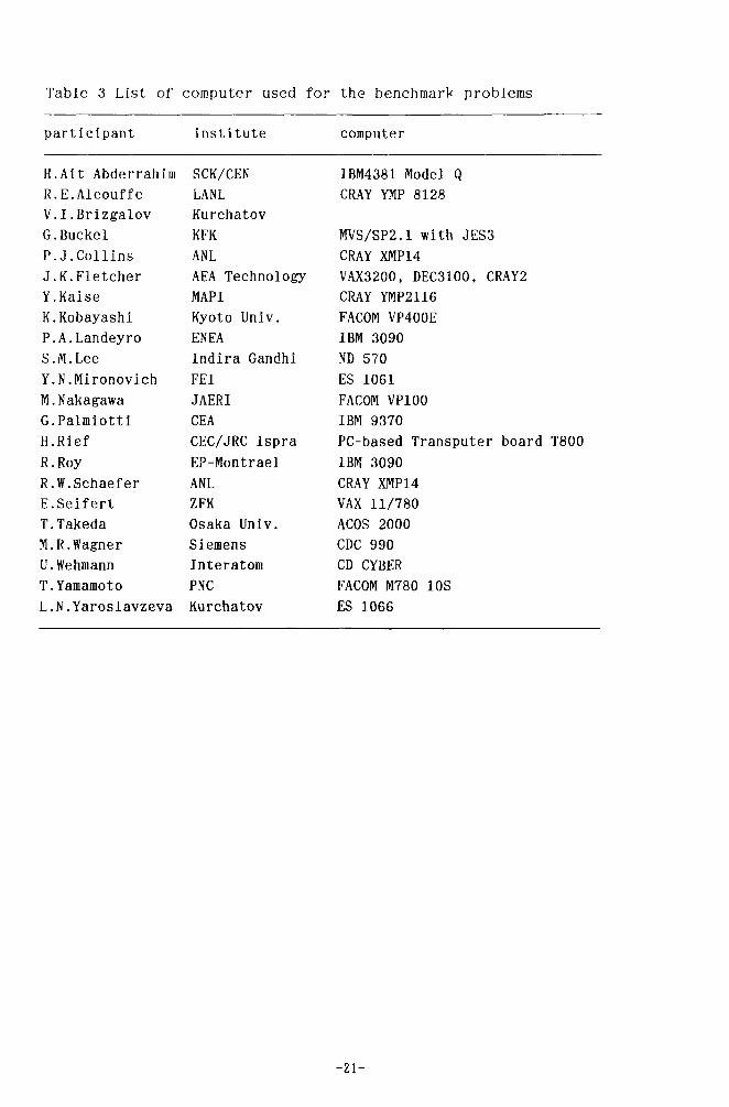
Table 3 List of computer used for the benchmark problems
participant institute computer
H.Ait Abderrahim
R.E.Alcouffe
V.I.Brizgalov
G.Buckel
P.J.Collins
J.K.Fletcher
Y.Kaise
K.Kobayashi
P.A.Landeyro
S.M.Lee
Y.N.Mironovich
M.Nakagawa
G.Palmiotti
H.Rief
R.Roy
R.W.Schaefer
E.Seifert
T.Takeda
M.R.Wagner
U.Wehmann
T.Yamamoto
L.N.Yaroslavzeva
SCK/CEN
LANL
Kurchatov
KFK
ANL
AEA Technology
MAPI
Kyoto Univ.
ENEA
Indira Gandhi
FEI
JAERI
CEA
CEC/JRC Ispra
EP-Montrael
ANL
ZFK
Osaka Univ.
Siemens
Interatom
PNC
Kurchatov
IBM4381 Model Q
CRAY YMP 8128
MVS/SP2.1 with JES3
CRAY XMP14
VAX3200, DEC3100, CRAY2
CRAY YMP2116
FACOM VP400E
IBM 3090
ND 570
ES 1061
FACOM VP100
IBM 9370
PC-based Transputer board T800
IBM 3090
CRAY XMP14
VAX 11/780
ACOS 2000
CDC 990
CD CYBER
FACOM M780 10S
ES 1066
-21-

Table 4 Average and control rod worth of Model 1
method
Exact Monte-Carlo
Monte-Carlo
Pn
S4
S8
CCRR
DOT3.5
case 1
0.9780
+0.0006
0.9778
+0.0005
0.9766
+0.0006
0.9766
+0.0002
0.J772
+.0.0001
0.9759
0.9836
case 2
0.9624
+0.0006
0.9624
+0.0005
0.9630
+0.0008
0.9622
+0.0002
0.9623
+0.0001
0.9622
0.9628
CR-worth
1.66E-02
+0.09E-02
1.64E-02
+0.07E-02
1.45E-02
+0.22E-02
1.54E-02
+0.01E-02
1.58E-02
+0.00E-02
1.46E-02
2.23E-02
Table 5 Averag-e and control rod worth of Model 2
method
Exact Monte-Carlo
Monte-Carlo
PnS4
S8
DIF3D(NTT)CCRR
case 1
0.9732
±0.0002
0.9731
+0.0002
0.9794
0.9735
±0.0001
0.9734
+0.0002
0.9714
0.9742
case 2
0.9594
+0.0002
0.9589
+0.0002
0.9647
0.9594
+0.0001
0.9593
+0.0002
0.9572
0.9596
CR-worth
1.47E-02
+0.03E-02
1.48E-02
+0.03E-02
1.56E-02
1.51E-02
+0.01E-02
1.52E-02
10.01E-02
1.54E-02
1.56E-02
-22-

Table G Average kGfj. and control rod worth of Model 3
method
Exact Monte-
Monte-Carlo
PnS4
S8
DIF3D(NTT)CCRR
case 1
Carlo
0.9709
+0.0002
0.9708
+0.0002
0.9772
0.9710
+0.0005
0.9704
+0.0004
0.9695
0.9673
case 2
1.0005
10.0002
1.0005
+0.0002
1.0040
1.0012
+0.0003
1.0006
±0.0004
0.9996
0.9968
case 3
1.0214
+0.0002
1.0214
10.0002
1.0247
1.0218
+0.0003
1.0213
+0.0005
1.0209
CR-worth
3.05E-02
+0.03E-02
3.06E-02
+0.03E-02
2.74E-02
3.11E-02
±0.04E-02
3.11E-02
10.03E-02
3.10E-02
3.06E-02
CRP-worth
2.03E-02
+0.00E-02
2.03E-02
+0.00E-02
2.01E-02
2.02E-02
+0.02E-02
2.03E-02
+0.02E-02
2.10E-02
Table 7 Average and control rod worth of Model 4
method case 1
Exact Monte-Carlo
Monte-Carlo
Pn
S8
HEXNOD(NT)CMEZ
1.0951
+0.0004
1.0951
+0.0004
1.0942
+0.0015
1.0887
±0.0043
1.0889
1.094
10.002
case 2
0.9833
10.0004
0.9833
i0.0004
0.9834
10.0055
0.9875
+0.0061
0.9783
0.980
+0.004
case 3
0.8799
10.0003
0.8799
10.0003
0.8819
10.0100
0.8927
10.0110
0.8748
0.881
10.002
CR-worth
2.23E-01
lO.OlE-01
2.23E-01
0.01E-01
2.20E-01
10.12E-01
2.02E-01
lO.lOE-01
2.25E-01
2.21E-01
10.30E-01
-23-

Table 8 Individual results of(Monte-Carlo method)
and control rod worth of Model 1
Bryzgalov
Rief
Landeyro
Seifert
Nakagawa
case 1
0.975+0.002
0.9780+0.000800.9781+0.00080
0.97946+0.00135
0.9773+0.0022
0.9776+0.00069
case 2
0.961±0.002
0.9627+0.000840.9628
±0.00084
0.96253±0.00138
0.9620+0.0022
0.9624+0.00071
CR-worth
1.494E-02+0.302E-02
1.G25E-02+0.120E-021.619E-02+0.120E-02
1.796E-02+0.205E-02
1.63E-02±0.31E-02
1.62E-02+0.102E-02
Table 9 Individual results of(Pn method)
and control rod worth of Model 1
PalmiottiPN = 7
FletcherPN=1PN=3PN=5PN=7
PN=7(half mesh)PN=7(zero mesh)
KobayashiPN=1PN = 3PN = 5PN inf*
case 1
0.97310
0.928310.969940.972240.972770.976070.97717
0.92340.97130.97430.9760
case 2
0.96131
0.931110.960330.961250.961370.963160.J6375
0.92980.96080.96170.9622
CR-worth
1.260E-02
-3.237E-031.032E-021.175E-021.218E-021.373E-021.424E-02
-7.454E-031.125E-021.345E-021.469E-02
• Extrapolated value
- 2 4 -

Table 10 Individual r e su l t s of(Sn method)
keff and control rod worth of Model 1
PalmiottiS8
BuckelDiffusionS4S8S16
LeeS6
AlcouffeS4S8S12S16S8(half mesh)
YaroslavzevaDif.S2
S4
S8
KaiseDif.S4
TakedaS4
S8
(1.(5.(2.(1.(5.(2.(1.(5.(2.(1.
(1.(0.(1.(0.
0cm)0cm)5cm)0cm)0cm)5cm)0cm)0cm)5cm)0cm)
0cm)5cm)0cm)5cm)
case 1
0
0000
0
0.0.0,0,0.
0.0.0.0.0.0.0.0.0.0.
0.0.
0.0.0.0.
.97711
.92771
.97668
.97713
.97723
.97729
.97670
.97714
.97721
.97723
.97719
,89998,976899782597861972279759397631972309766297711
927319766
97669976699771397713
case 2
0
0000
0
0000.0
0,0,0.0.0.0.0.0.0.0.
0.0.
0.0.0.0.
.96230
.93113
.96231
.96231
.96223
.96250
.96236
.96236
.96231
.96228
.96246
.91952
.95755
.96116
.96207
.95588
.96112
.96198,955329613896229
930399619
96232962249622996238
CR-worth
1
-3111
1
11111
-2211111111
-31
1111
.575E-02
.949E-02
.528E-02
.576E-02
.595E-02
.572E-02
.526E-02
.572E-02
.585E-02
.590E-02
.566E-02
.36E-02
.06E-02
.82E-02
.76E-02
.76E-02
.58E-02
.53E-02
.83E-02
.62E-02
.58E-02
.570E-02
.56E-02
.529E-02
.538E-02
.578E-02
.569E-02
- 2 5 -

Table 11 Individual results of(Other methods)
and control rod worth of Model 1
Ait AbderrahimD0T3.5(Synthesis)
PalmiottiCCRR*CCRR**
RoyDRAGON ICI
IC2IC3CP1CP2LAGR2LAGR3MCFD2MCFD3
case 1
0
00
011010000
.98365
.97589
.96328
.94840
.07864
.13533
.89430
.00645
.93220
.92832
.92466
.92864
case 2
0.96283
0.962210.94794
0.925221.055911.115190.874350.987240.936570.932590.928380.93230
CR-worth
2.
1.1.
2.1.1.2.1.
-3.-4.-4.-4.
229E-02
457E-02680E-02
642E-02995E-02590E-02551E-02934E-02725E-02930E-03343E-03221E-03
***ICIIC2IC3CP1CP2LAGR2
LAGR3
Combination of 3D diffusion and 2D transport 'BISTRO'Used transport equivalent cross-sectionThe first IC solutionThe first IC solutionThe first IC solutionno used IC techniqeno used IC techniqe
considered 5x5x5 cm0
considered 2.5x2.5xJconsidered lxlxl
block.5 cm^ blockblock
considered 5x5x5 cm^ blocconsidered 2.5x2.5x2.5 craa block
the variational collocation method on diffusion equationwith quadratic Lagrange polynomials expansion.the variational collocation method on diffusion equationwith cubic Lagrange polynomials expansion.
-26-

Table 12 Individual results of(Monte-Carlo method)
and control rod worth of Model 2
Wehmann
Schaefer
Rief
Landeyro
Bryzgalov
Seifert
Nakagawa
case 1
0±0
0
±0
0
±0
0±0
0+0
0±0
0
±0
.97298
.000315
.97344
.000363
.9732
.00047
.97285
.00079
.9707
.0012
.9729
.0015
.9732
.00048
case 2
0.±o.
0.±o.
0.
0.±o.
0.±o.
0.
±0-
0.+0.
95919000326
95988000384
9591
9592200077
95300007
95750016
959300042
CR-worth
1.478E-02i0.049E-02
1.451E-02+0.057E-02
1.511E-02+0.063E-02
1.461E-02+0.118E-02
1.913E-02i0.781E-02
1.65E-02+0.22E-02
1.49E-020.066E-02
Table 13 Individual results of(Pn method)
and control rod worth of Model 2
FletcherPN=1PN=3PN=5PN = 7
PN=7(halfPN=7(zero
mesh)mesh)
case 1
0.978540.982970.983040.983050.980210.97936
case 2
0.964750.969820.969910.969930.965970.96465
CR-worth
1.461E-021.372E-021.377E-021.377E-021.504E-021.556E-02
- 2 7 -

Table 14 Individual results of(Sn method)
and control rod worth of Model 2
BuckelDif.S4S8S16
AlcouffeS4SSS12S16S8(half mesh)
LeeS8
YaroslavzevaDif.S2S4S8
YamamotoS4S8
KaiseDif.S4
TakedaS4(5.0cm)
(2.5cm)S8(5.0cm)
(2.5cm)
case 1
0000
00000
0
0000
00
00
0000
.95460
.97321
.97341
.97345
.97348
.97348
.97348
.97348
.97360
.97311
.96494
.97344
.97359
.97347
.97344
.97345
.97058
.9736
.97361
.97341
.97361
.97339
case 2
0.938060.959230.959250.95927
0.959360.959310.959300.959300.95954
0.95899
0.952240.959000.959390.95924
0.959270.95922
0.957420.9594
0.959610.959340.959560.95928
CR-worth
1.847E-021.498E-021.516E-021.518E-02
1.511E-021.517E-021.518E-021.519E-021.506E-02
1.513E-02
1.38E-021.55E-021.52E-021.52E-02
1.518E-021.524E-02
1.416E-021.520E-02
1.498E-021.507E-021.504E-021.511E-02
- 2 8 -

Table 15 Individual results of(Other methods)
and control rod worth of Model 2
PalmlottiCCRR*CCRR**
CollinsDIF3D NDT
NTT
RoyDRAGON ICI
IC2
case 1
0.974220.96839
0.969110.97143
0.994510.95558
case 2
0.959610.95394
0.954350.95716
0.978780.94031
CR-worth
1.563E-021.564E-02
1.596E-021.535E-02
1.616E-021.699E-02
*«NDTNTTICIIC2
Combination of 3D diffusion and 2D transportUsed transport equicvalent cross-sectionNodal Diffusion TheoryNodal Transport TheoryThe first IC solution; considered 5x5x5 cm blookThe first IC solution; considered 2.5x2.5x2.5 cm"* blook
-29-

Table 16 Individual results of ke f f
(Monte-Carlo method)and control rod worth of Model 3
Wehmann
Rief
Schaefer
Landeyro
Nakagawa
case 1
0.97059+0.000306
0.96767+0.0014
0.97089±0.000317
0.97169+0.00069
0.9712+0.00054
case 2
1.00063+0.000296
0.99721
1.00059±0.000343
1.00068+0.00075
0.9998+0.00065
case 3
1.02131±0.000298
1.02142±0.000341
1.02091±0.00072
1.0216±0.00058
CR-worth
3.093E-02+0.044E-02
3.0612E-02+0.0605E-02
3.057E-02±0.048E-02
2.9814E-02±0.105E-02
2.94E-02+0.086E-02
CRP-worlh
2.024E-02+0.00049E-02
2.039H-02±0.00047K-02
1.980E-02+0.102E-02
2.13E-02±0.086E-02
Table 17
FletcherPN = 1PN = 3PN=5PN = 7
PN=3(half
Individual results of k o ^(Pn method)
case 1
0.970720.968440.977120.97716
mesh) 0.97298
case 2
0.998761.003751.003991.004021.00177
? and control
case 3
1.020361.024571.024691.024701.02277
rod worth
CR-worth
2.892E-023.633E-022.739E-022.738E-022.954E-02
of Model 3
CRP-worth
2.119E-022.024E-022.012E-022.009E-022.049E-02
- 3 0 -

Table 18 Individual results of(Sn method)
and control rod worth of Model 3
case 1 case 2 case 3 CR-worth CRP-worth
AlcouffeS4S8S12S16S8(half mesh]
BuckelDiff.S4S8S16
YaroslavzevaDif.S2S4S8
LeeS4S8
0.970600.969990.969910.969870.97035
0.952670.971470.970840.97076
0.968500.958170.970870.97025
0.97000.9697
1.001291.000801.000731.000701.00091
0.986671.001331.000831.00076
0.996430.997681.001391.00067
1.00050.9996
1.021841.021421.021341.02133
1.00S651.021971.021461.02142
1.018531.018461.021921.02117
1.02121.0202
158E-02174E-02176E-02177E-02
3.147E-02
3.6169E-023.0703E-023.0857E-023.0886E-02
2.89E-024.13E-023.14E-023.13E-02
3.143E-023.085E-02
2.009E-022.017E-022.017E-022.018E-02
2.208E-022.017E-022.019E-022.021E-02
2.178E-022.045E-022.006E-022.006E-02
2.026E-022.020E-02
YamamotoS4S8
TakedaS4S8
0.971350.97076
0.971420.97081
1.001211.00071
1.001271.00077
1.021831.02135
1.021891.02140
3.070E-023.083E-02
3.069E-023.084E-02
2.016E-022.019E-02
2.015E-022.018E-02
-31-

Table 19 Individual results of(Other methods)
and control rod worth of Model 3
CollinsDIF3D NDT
NTT
PalmiottiCCRR*CCRR**
RoyDRAGON ICI
case 1
0.964810.96951
0.961350.96733
0.98547
case 2
0.995690.99955
0.994780.99684
1.01854
case 3
1.017691.02091
1.01697
1.03208
CR-worth
3.214E-023.100E-02
3.496E-023.060E-02
3.396E-02
CRP-worth
2.171E-022.093E-02
2.193E-02
1.288E-02
NDT : Nodal Diffusion TheoryNTT : Nodal Transport Theory* : Combination of 3D diffusion and 2D transport•* : Used transport equicvalent cross-sectionICI : The first IC solution; considered 5x5x5 cm3 blook
-32-

Table 20 Individual results of(Monte-Carlo method)
and control rod worth of Model 4
'. chmann
Bryzgalov
Seifert
Nakagawa
case 1
1±0
1±0
1±0
1±0
.09515
.000395
.096
.002
.0960
.0023
.0947
.00086
case 2
0.98340+0.000394
0.981+_0.002
0.9860+.0.0021
0.9825+0.0014
case 3
0.88001±0.000375
0.878+0.002
0.8806+0.0019
0.8794+0.00084
CR-worth
2.232E-01+.0.0059E-01
2.265E-0110.031E-01
2.232E-01+0.030E-01
2.236E-01+0.012E-01
Table 21 Individual results of(Pn method)
and control rod worth of Model 4
PalmlottiPN=1PN=3PN=5PN=7
FletcherPN=1PN=3PN=5PN=7
PN=7(half mesh)PN=7(zero mesh)
case 1
1.07860
1.095631.09570
1.078601.095581.095631.095701.093471.09273
case 2
0.970710.988630.988890.98892
0.970710.988630.988920.988920.980600.97782
case 3
0.87217
0.89203
0.872170.891660.892010.892030.876780.87170
CR-worth
2.194E-01
2.084E-01
2.194E-012.088E-012.083E-012.084E-012.260E-012.320E-01
- 3 3 -

Table 22 Individual results of(Sn method)
and control rod worth of Model 4
YaroslavzevaDif.S2S4S8
TakedaS4*S4**S8*
case 1
1.095881.106701.093231.09303
1.084381.C88791.08436
case 2
1.007270.997850.994180.99359
0.982140.971980.98145
case 3
0.937730,918970.904150.90360
0.881320.858420.88179
CR-worth
1.539E-011.846E-011.913E-011.918E-01
2.125E-012.465E-012.119E-01
• : calculated by HEX-Z1 code•• : calculated by HEZ-Z2 code
Table 23 Individual results of(Other r-3thods)
and control rod worth of Model 4
MironovichCMEZ(Synthesis)
WagnerHEXNOD DT 12
20NT 12
20
case 1
1.094+0.002
1.077151.076671.089191.08890
case 2
0.980+0.004
0.961300.960820.978510.97830
case 3
0.881+0.002
0.852930.852930.874650.87484
CR-worth
2.21E-01+.0.30E-01
2.4405E-012.4363E-012.2521E-012.2470E-01
CMEZ : Combination method codeDT : Diffusion theoryNT : Nodal transport theory, with DPj approximation at node interfaces12 & 20 : Number of axial layer
-34-
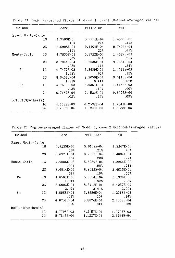
Table 24 Region-averaged fluxes of Model 1, easel (Method-averaged values)
method
Exact Monte-Carlo1G
2G
Monte-Carlo 1G
2G
Pn 1G
2G
Sn 1G
2G
D0T3.5(Synthesis)1G2G
core
4.7509E-03.10%
8.6998E-04.12%
4.7835E-03.06%
8.7841E-04.08%
4.7472E-031.22%
8.6452E-041.21%
4.7650E-03.03%
8.7162E-04.02%
4.6082E-038.7682E-04
reflector
5.9251E-04.21%
9.1404E-04.23%
5.9722E-04.08%
9.2036E-04.11%
5.9439E-04.92%
9.2059E-043.44%
5.9361E-04.10%
9.1520E-04.24%
6.2502E-041.1900E-03
void
1.4500E-03.47%
9.7406E-04.63%
1.4529E-03.21%
9.7684E-04.34%
1.4096E-03.19%
9.0113E-043.62%
1.4453E-03.06%
9.6997E-04.09%
1.7341E-031.3088E-03
Table 25 Region-averaged fluxes of Model 1, case 2 (Method-averaged values)
method
Exact Monte-Carlo
Monte-Carlo
Pn
Sn
1G
2G
1G
2G
1G
2G
1G
2G
DOT3.5(Synthesis)1G2G
core
4.9125E-03.10%
8.6921E-04.13%
4.9006E-03.06%
8.6814E-04.08%
4.8581E-031.91%
8.6003E-042.07%
4.8968E-03.03%
8.6751E-04.02%
4.7795E-038.7145E-04
reflector
5.9109E-04.21%
8.7897E-04.23%
5.8989E-04.08%
8.8012E-04.10%
5.8854E-041.82%
8.8412E-043.41%
5.8980E-04.10%
8.8074E-04.31%
6.2157E-041.1227E-03
1
2
1
2
1
2
1
2
12
CR
.2247E-03.48%
.4604E-04.72%
.2264E-03.21%
.4615E-04.35%
.1996E-03.08%
.4257E-042.99%
.2218E-03.14%
.4538E-04.18%
.3707E-03
.9764E-04
- 3 5 -

Table 26 Region-averaged fluxes of Model 2, case 1 (Method-averaged values)
method
Exact Monte-Carlo1G
2G
3G
4G
Monte-Carlo 1G
2G
3G
4G
Pn 1G2G3G4G
Sn 1G
2G
3G
4G
D1F3D(NTT) 1G2G3G4G
DOT3.5(Synthesis)1G2G3G4G
core
4.2814E-05.06%
2.4081E-04.05%
1.6411E-04.06%
6.2247E-06.20%
4.2817E-05.06%
2.4083E-04.05%
1.6409E-04.06%
6.2214E-06.19%
4.2370E-052.3926E-041.6679E-046.2855E-064.2815E-05
.02%2.4072E-04
.05%1.6405E-04
.02%6.2113E-06
.05%4.2766E-052.4059E-041.6406E-046.2147E-06
4.0369E-052.3970E-041.7128E-046.5905E-06
radialblanket
3.3252E-06.18%
3.0893E-05.10%
3.2834E-05.10%
2.0473E-06.34%
3.3249E-06'7%
3.087^,-05.10%
3.2817E-05.10%
2.0487E-06.33%
3.5595E-063.5354E-054.0261E-052.6785E-053.3494E-06
.05%3.1192E-05
.02%3.3091E-05
.10%2.0582E-06
.16%3.4022E-063.1169E-053.3012E-052.0559E-06
3.2489E-063.1736E-053.4866E-052.2U9E-06
axialblanket
5.1850E-06.27%
4.6912E-05.14%
4.6978E-05.16%
3.7736E-06.46%
5.1835E-06.26%
4.6902E-05.13%
4.6959E-05.15%
3.7578E-06.43%
5.4492E-065.3696E-055.7551E-055.0063E-065.2125E-06
.08%4.7407E-05
.05%4.7324E-05
.15%3.7513E-06
.21%5.2868E-064.7367E-054.7206E-053.7529E-06
4.9696E-064.7186E-054.8817E-053.8902E-06
CRP
2.5344E-05.33%
1.6658E-04.18%
1.2648E-04.23%
6.9840E-06.17%
2.5362E-05.32%
1.6678E-04.18%
1.2652E-04.22%
6.9834E-06.17%
2.5130E-051.6795E-041.3187E-047.9182E-062.5559E-05
.04%1.6696E-04
.on1.2677E-04
.04%6.9202E-06
.18%2.5584E-051.6646E-041.2653E-046.9475E-06
2.5241E-051.7317E-041.3650E-047.3544E-06
- 3 6 -
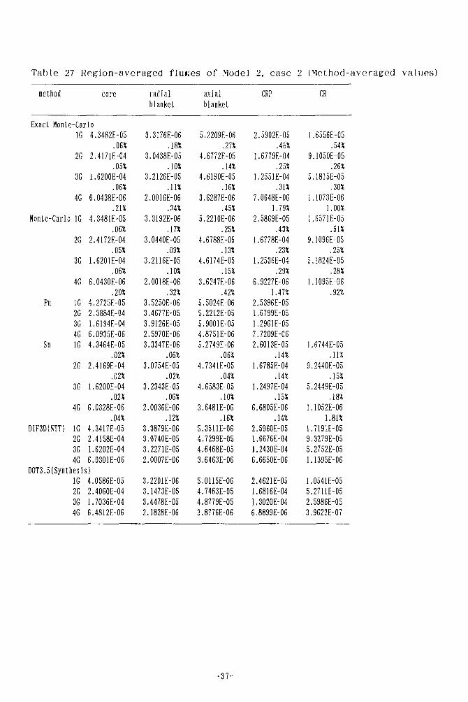
Table 27 Region-averaged fluKes of Model 2, case 2 (Method-averaged values)
method core
Exact Monte-CarloIG
2G
3G
4G
Monte-Carlo 1G
2G
3G
4G
Pn 1G2G3G4G
Sn IG
2G
3G
4G
DIF3D(NTT) 1G2G3G4G
4.3482E-05.063!
2.4171E-04.05%
1.6200E-04.06%
6.0438E-06.21*
4.3481E-05.06*
2.4172E-04.05*
1.6201E-04.06*
6.0430E-06.20*
4.2725E-052.3884E-041.6194E-046.0935E-064.3464E-05
.02*2.4169E-04
.02*1.6200E-04
.02*6.0328E-06
.04*4.3417E-052.4158E-041.6202E-046.0301E-06
DOT3.5(Synthesis)1G2G3G4G
4.0586E-052.4060E-041.7036E-046.4812E-06
3
3
3
2
3
3
3
2
3,3,3,2.3.
3.
3.
2.
3.3.3.2.
3.3.3.2.
radialblanket
.3176E-06.18*
.0438E-05.10*
.2126E-05.11*
.0016E-06.34*
.3192E-06.17*
.0440E-05.09*
.2116E-05.10*
.0018E-06.32*
.5250E-06•4677E-05.9126E-05. 5970E-06.3347E-06
.06*0754E-05
.02*2343E-05
.06*0036E-06
.12*3879E-060740E-052271E-050007E-06
2201E-061473E-054478E-051828E-06
5
4
4
3
5
4
4
3
555,4.5.
4.
4.
3.
5.4.4.3.
5.4.4.3.
axialblanket
.2209E-06.27*
.6772E-05.14*
.6190E-05.16*
.6287E-06.45*
.2210E-06.25*
.6788E-05.13*
.6174E-05.15*
.6247E-06.42*
.5024E-06
.2212E-05
.9001E-05
.8751E-06
.2749E-06.06*
7341E-05.04*
6583E-05.10*
6481E-06.16*
3511E-067299E-056468E-056463E-06
0115E-067463E-058779E-058776E-06
2
1
1
7
2
1
1
6
2,11,1,2.
1.
1.
6.
2.1.1.6.
2.1.1.6.
CRP
.5902E-05.46*
.6779E-04.25*
.2551E-04.31*
.0648E-061.79*
.5869E-05.43*
.6778E-04.23*
.2536E-04.29*
.9227E-061.47*
.5396E-05
.6799E-05
.2961E-05
.7209E-06
.6013E-05.14*
6785E-04.14*
2497E-04.15*
6805E-06.14*
5960E-056676E-042430E-046650E-06
4621E-056816E-043020E-048899E-06
CR
1.6556E-05.54*
9.1050E-05.26*
5.1815E-05.30*
1.1073E-061.00*
1.6571E-05.51*
9.1096E-05.25*
5.1824E-05.28*
1.1095E-06.92*
1.6744E-05.11*
9.2440E-05.15*
5.2449E-05.18*
1.1052E-061.81*
1.7191E-059.3279E-055.2752E-051.1395E-06
1.0541E-055.2711E-052.5986E-053.9622E-07
-37 -

Table 28 Region-averaged fluxes of Model 3, case 1 (Method-averaged values)
method core
Exact Monte-Carlo1G
2G
3G
4G
Monte-Carlo1G
2G
3G
4G
Pnill
1G2G3G4G
Cnoil
1G
2G
3G
4G
DIF3D(NTT)1G2G3G4G
2.0334E-0S.06%
1.1501E-04.04*
8.2784E-05.05*
3.4093E-06.19%
2.0334E-05.06*
1.1501E-04.04*
8.2782E-05.05*
3.4093E-06.19*
2.0391E-051.1513E-048.2809E-053.401SE-06
2.0377E-05.02*
1.1495E-04.03*
8.2653E-0S.03*
3.3994E-06.07*
2.0336E-051.1490E-048.2713E-053.4001E-06
internalblanket
1.2562E-05.35*
1.1237E-04.20*
1.1931E-04.22*
7.4318E-06.65*
1.2552E-05.34*
1.1232E-04.20*
1.1923E-04.22*
7.4326E-06.63*
1..1947E-051.0971E-041.1888E-047.5803E-06
1.2598E-05.08*
1.1260E-04.05*
1.1958E-04.05*
7.4321E-06.05*
1.2802E-051.1296E-041.1968E-047.4302E-06
radialblanket
1.5888E-06.36*
1.6736E-05.22*
2.1521E-05.22*
1.7973E-06.56*
1.5903E-06.36*
1.6749E-05.22*
2.1532E-05.22*
1.7995E-06.56*
1.5541E-061.6582E-052.1690E-051.8549E-06
1.6067E-06.04*
1.6799E-05.05*
2.1600E-05.09*
1.8086E-06.18*
1.6391E-061.6829E-052.1524E-051.7929E-06
axialblanket
2.9405E-06.23*
3.0115E-05.12*
3.5408E-05.13*
3.7516E-06.32*
2.94Û5E-06.23*
3.0113E-05.12*
3.5406E-05.13*
3.7519E-06.32*
2.8687E-063.0770E-053.7543E-054.1841E-06
2.9599E-06.35*
3.0253E-05.37*
3.5486E-05.41*
3.7661E-06.44*
2.9909E-063.0320E-053.5528E-053.7686E-06
CRP
1.2230E-05.20*
8.6309E-05.11*
7.5128E-05.12*
5.3074E-06.43*
1.2233E-05.20*
8.6332E-05.11*
7.5154E-05.12*
5.3099E-06.43*
1.3244E-059.2081E-057.7626E-055.5562E-06
1.2244E-0S.59*
8.6200E-05.63*
7.4726E-05.75*
5.2587E-06.86*
1.2304E-058.6401E-057.5019E-055.2973E-06
CR
1.2150E-05.45*
6.7771E-05.22*
3.9699E-05.25*
8.6717E-07.83*
1.2116E-05.45*
6.7576E-05.22*
3.9637E-05.25*
8.6972E-0?.83*
1.2624E-056.8328E-057.9238E-058.3664E-07
1.2347E-05.08*
6.8586E-05.10*
4.0117E-05.15*
8.5409E-07.60*
1.2666E-056.9125E-054.0361E-058.8696E-07
-38-

Table 29 Region-averaged fluxes of Model 3, case 2 (Method-averaged values)
method core
Exact Monte-Carlo1G
2G
3G
4G
Monte-Carlo1G
2G
3G
4G
Pnrn
1G2G3G4G
Sn1G
2G
3G
4G
DIF3D(NTT)1G2G3G4G
1.9859E-05.06*
1.1439E-04.04%
8.4521E-05.05%
3.5472E-06.195;
1.9859E-05.06%
1.1439E-04.04*
8.4521E-05.05%
3.5472E-06.19%
1.9932E-051.1465E-048.4426E-053.5258E-06
1.9868E-05.05%
1.1437E-04.04%
8.4481E-05.06%
3.5423E-06.09%
1.9825E-051.1430E-048.4534E-053.5481E-06
internalblanket
1.2267E-05.32%
1.1272E-04.21%
1.2240E-04.21%
7.7910E-06.64%
1.2267E-05.32%
1.1272E-04.21%
1.2240E-04.21%
7.7910E-06.64%
1.1774E-051.1041E-041.2213E-047.8906E-06
1.2384E-05.25%
1.1321E-04.28%
1.2309E-04.39%
7.7809E-06.45%
1.2609E-051.1377E-041.2346E-047.8077E-06
radialblanket
1.5266E-06.39%
1.6168E-05.23%
2.0996E-05.22%
1.7728E-06.54%
1.5266E-06.39%
1.6168E-05.23%
2.0996E-05.22%
1.7728E-06.54%
1.4835E-061.6070E-052.Î299E-051.8178E-06
1.5260E-06.55%
1.6236E-05.58%
2.21ME-05.83%
1.7745E-061.11%
1.5534E-061.6217E-052.0952E-051.7495E-06
axialblanket
2.8785E-06.24%
2.9877E-05.13%
3.5685E-05.13%
3.8246E-06.33%
2.8785E-06.24%
2.9877E-05.13%
3.5685E-05.13%
3.8246E-06.33%
2.8004E-063.0601E-053.7848E-054.2348E-06
2.8798E-06.31%
3.0022E-05.34%
3.5792E-05.36%
3.8238E-06.41%
2.9106E-063.0111E-053.5856E-053.8289E-06
CRP
1.2522E-05.19%
8.8832E-05.10%
7.7412E-05.12%
5.3470E-06.42%
1.2522E-05.19%
8.8832E-05.10%
7.7412E-05.12%
5.3470E-06.42%
1.2575E-05.36%
8.8972E-05.39%
7.7302E-05.50%
5.2992E-06.58%
1.2641E-058.9197E-057.7653E-055.3470E-06
- 3 9 -

Table 30 Region-averaged fluxes of Model 3, case 3 (Method-averaged values)
method core
Exact Monte-CarloIG
2G
3G
4G
Monte-Carlo1G
2G
3G
4G
Pn1G2G3G4G
Sn1G
2G
3G
4G
DIF3D(NTT)IG2G3G4G
1.9033E-05.06%
1.1026E-04.04%
8.0177E-05.05»
3.1958E-06.19%
1.9033E-05.06%
U026E-04.04%
8.0177E-05.05%
3.1958E-06.19%
1.9106E-051.1046E-048.0112E-043.1694E-06
1.9048E-05.05%
1.1023E-04.04%
8.0153E-05.06%
3.1862E-06.08%
1.9007E-051.1017E-048.0215E-053.1913E-06
D0T3.5(Synthesis)1G2G3G4G
1.8530E-051.0458E-047.7395E-053.2295E-06
internalblanket
1.1875E-05.35%
1.0838E-04.21%
1.1672E-04.22%
7.0366E-06.67%
1.1875E-05.35%
1.0838E-04.21%
1.1672E-04.22%
7.0366E-06.67%
1.1920E-05.28%
1.0858E-04.32%
1.1679E-04.43%
7.0488E-06.49%
1.2097E-051.0901E-041.1713E-047.0760E-06
4.5322E-064.3552E-055.4533E-053.8575E-06
radialblanket
1.3718E-06.38%
1.4703E-05.22%
1.S121E-05.23%
1.6164E-06.57%
1.3718E-06.38%
1.4703E-05.22%
1.9121E-05.23%
1.6164E-06.57%
1.3751E-06.65%
1.4805E-05.68%
1.9327E-05.99%
1.6244E-061.29%
1.3955E-061.4753E-051.9129E-051.5970E-06
2.7072E-062.8030E-053.6439E-053.1295E-06
axialblanket
2.7276E-06.24%
2.8409E-05.13%
3.3614E-05.13%
3.5169E-06.33%
2.7276E-06.24%
2.8409E-05.13%
3.3614E-0S.13%
3.5169E-06.33%
2.6435E-062.8839E-053.5362E-053.8573E-06
2.7272E-06.35%
2.8423E-05.39%
3.3655E-05.39%
3.5175E-06.42%
2.7486E-062.8450E-053.3663E-053.5173E-06
2.3309E-062.3692E-052.9089E-053.2220E-06
- 4 0 -

Table 31 Region-averaged fluxes of Model 4, case 1 (Method-averaged values)
lethod testzone
Exact Monte-Carlo1G
2G
3G
4G
Monte-Carlo1G
2G
3G
4G
Pn1G2G3G4G
Sn1G2G3G4G
HEXNOD(NT)1G2G3G4G
1.3499E-04.11%
1.085GE-04.14*
3.0770E-05.24*
3.8749E-06.442;
1.3499E-04.11%
1.0856E-04.14%
3.0770E-05.24%
3.8749E-06,44%
1.3246E-041.0884E-043.1356E-053.9845E-06
1.3435E-051.0791E-043.0289E-053.2917E-06
1.3317E-041.0741E-043.0910E-053.9903E-06
axialblanket
3.5243E-05.24%
4.9804E-05.23%
2.6203E-05.35%
1.2749E-05.32%
3.5243E-05.24%
4.9804E-05.23%
2.6203E-05.35%
1.2749E-05.32%
3.8626E-055.3507E-052.7845E-051.2776E-05
3.5410E-054.9618E-052.5893E-051.1649E-05
3.5860E-054.9930E-052.6255E-051.2073E-05
driver withioderator
6.3396E-05.09%
4.9993E-05.08%
2.8215E-05.10%
1.4486E-05.11%
6.3396E-05.09%
4.9993E-05.08%
2.8215E-05.10%
1.4486E-05.11%
6.3676E-054.8661E-052.7724E-051.4261E-05
6.6393E-055.1327E-052.8424E-051.4341E-05
6.5622E-055.0333E-052.8358E-051.4532E-05
CRP
5.2497E-05.11%
5.0666E-05.12%
2.2G37E-05.20%
1.0366E-05.34%
5.2497E-05.11%
5.06G6E-05.12%
2.2637E-05.20%
1.0366E-05.34%
5.3900E-055.1974E-052.3449E-051.1151E-05
5.4226E-055.1474E-052.2143E-059.2927E-06
5.2673E-055.0610E-052.2703E-051.0527E-05
- 4 1 -

Table 32 Region-averaged fluxes of Model 4, case 2 (Method-averaged values)
•ethod testzone
Exact Monte-Carlo1G
2G
2o
4G
Monte-Carlo1G
2G
3G
4G
r n1G2G3G4G
ÇTI
bn1G2G3G4G
HEXNOD(NT)1G2G3G4G
1.4695E-04.10%
1.1251E-04.12%
2.6560E-05.24%
2.4518E-06.35%
1.4695E-04.10%
1.1251E-04.12%
2.6560E-05.24%
2.4518E-06.35%
1.4619E-041.1202E-042.G725E-052.6008E-06
1.4946E-041.1226E-042.5243E-052.0788E-06
1.4733E-041.1149E-042.6463E-052.5308E-06
axialblanket
3.7122E-05.22%
4.87S8E-05.21%
2.2353E-05.35%
8.6G71E-0G.59%
3.7122E-05.22%
4.8758E-05.21%
2.2353E-05.35%
8.6671E-06.59%
4.0153E-055.1692E-052.3587E-059.2026E-06
3.7525E-054.8811E-052.2012E-058.4655E-06
3.7583E-054.8760E-052.2502E-058.7327E-06
driver with•oderator
7.0291E-05.08%
5.1347E-05.09%
2.7720E-05.10%
1.3952E-05.12%
7.0291E-05.08%
5.1347E-05.09%
2.7720E-05.10%
1.3952E-05.12%
6.9230E-055.0327E-052.7600E-051.3969E-05
7.1443E-055.2295E-052.7650E-051.3793E-05
7.0620E-055.1532E-0S2.7810E-051.3965E-05
CRP
1.1866E-04.14%
1.0031E-04.16%
3.6997E-05.27%
1.1076E-05.48%
1.1866E-04.14%
1.0031E-04.16%
3.6997E-05.27%
1.1076E-05.48%
1.1947E-049.9713E-053.7225E-051.1472E-05
1.2547E-041.0395E-053.6876E-059.1418E-06
1.1912E-049.9954E-053.7343E-051.1241E-05
CR
4.4354E-05.17%
3.5773E-05.18%
7.7894E-06.32%
4.8143E-07.43%
4.4354E-05.17%
3.5773E-05.18%
7.7894E-06.32%
4.8143E-07.43%
4.5836E-053.6277E-051.2536E-053.8632E-06
4.7178E-053.7692E-058.1131E-064.9955E-07
4.4890E-053.5967E-057.7973E-066.2915E-07
- 4 2 -

Table 33 Region-averaged fluxes of Model 4, case 3 (Method-averaged values)
method testzone
Exact Monte-Carlo1G
2G
3G
4G
Monte-Carlo1G
2G
3G
Pn1G?G?G4G
Sn1G2G3G4G
HEXNOD(NT)1G2G3G4G
1.4983E-04.11*
1.1677E-04.14*
2.1823E-05.29%
1.1863E-06.41*
1.4983E-04.11%
1.1677E-04.14*
.295;i.)S63E-O6
.415!
:.: .:;£-042.1475E-051.2197E-07
1.6885E-041.1766E-041.9566E-059.8209E-05
1.6465E-041.1G40E-042.1815E-O51.1923E-05
axialblanket
4.0B60E-05.24*
5.1828E-05.23*
2.3632E-05.36*
9.8501E-06.43*
4.0660E-05.24*
5.1828E-05.23*
2.3632E-05.36*
9.8501E-06.43*
4.3773E-055.5105E-052.4826E-051.0372E-05
4.1747E-065.2949E-052.3442E-059.5603E-06
4.1S37E-055.2117E-052.3668E-059.7162E-06
driver with•oderator
7.4993E-05JO*
5.1904E-05.10*
2.6958E-05.11*
1.3391E-0S.13*
7.4993E-05.10*
5.1904E-05.10*
2.6958E-05.11*
1.3391E-05.13*
7.4091E-055.1229E-052.7126E-051.3616E-05
7.6295E-055.2631E-052.6580E-051.3210E-05
7.5255E-055.2147E-052.7023E-051.3396E-05
CR
9.5471E-05.10*
6.9316E-05.11*
1.3437E-05.21*
9.5265E-07.40*
9.5471E-05.10*
6.9316E-05.11*
1.3437E-05.21*
9.5265E-07.40%
9.6475E-056.8633E-051.2895E-058.2098E-07
1.0559E-047.5813E-051.4578E-057.8467E-07
9.6537E-056.9708E-051.3615E-041.0023E-06
- 4 3 -

Table 34 Individual results of region-averaged fluxes of Model 1, case 1(Monte-Carlo method)
Rief
Landeyro
Bryzgalov
Seifert
Nakagawa
1G
2G
1G
2G
1G
2G
1G
2G
1G
2G
core
4.8010E-03.07%
8.7918E-04
.10%4.6924E-03
.26%8.6762E-04
.36%4.7774E-03
8.7487E-04
4.763E-03
.25%8.707E-03
.40%4.7617E-03
.11%8.7029E-04
.13%
reflector
5.9845E-04.09%
9.2268E-04.13%
5.9318E-04.42%
9.1387E-04.52*
5.9795E-04
9.1795E-04
5.916E-04
.35%9.177E-04
.50%5.9227E-04
.25%9.1408E-04
.25%
void
1.4536E-03.23%
9.7804E-04.41%
1.4528E-031.17%
9.5522E-041.35%
1.4462E-03
S.6410E-04
1.4495E-03.51%
9.7954E-04.71%
Table 35 Individual results of region-averaged fluxes of Model 1, case 1(Pn method)
core reflector void
Palmiotti 1G2G
KobayashI 1G2G
Fletcher 1G2G
4.8277E-038.6979E-044.6949E-038.7392E-044.7191E-038.4987E-04
6.0181E-049.5267E-045.9248E-048.7744E-045.8890E-049.3166E-04
1.4122E-038.6851E-041.4069E-039.3375E-04
-44-

Table 36 Individual results of region-averaged fluxes of Model 1, case 1(Sn method)
Alcouffe
Buckel
Lee
Yaroslavzeva
Takeda
1G2G1G2G
1G2G1G2G1G2G
4848484848
core
.7652E-03
.7174E-04
.7643E-03
.7142E-04
.7835E-03
.7180E-04
.7657E-03
.7173E-04
.7666E-03
.7152E-04
reflector
5.9387E-04
9.1554E-04
5.9434E-04
9.1637E-04
5.9391E-04
9.1813E-04
5.9356E-04
9.1233E-04
5.9265E-04
9.1398E-04
void
1.4458E-03
9.7080E-04
1.4462E-03
9.7147E-04
1.4447E-03
9.6989E-04
1.4460E-03
9.6951E-04
1.4441E-03
9.G902E-04
Table 37 Individual results of region-averaged fluxes of Model 1, case 1(Other methods)
core reflector void
Ait Abderrahim (Synthesis method)1G 4.6082E-03 6.2502E-04 1.7341E-032G 8.7682E-04 1.1900E-03 1.3088E-03
- 4 5 -

Table 38 Individual results of region-averaged fluxes of Model 1, case 2(Monte-Carlo method)
Rief
Landeyro
Bryzgalov
Seifert
Nakagawa
1G
2G
1G
2G
1G
2G
1G
2G
1G
2G
4.
8.
5.
8.
4.
8.
4
8
4.
8.
core
8956E-03. 07%
6766E-04.10%
0450E-03.35%
7717E-04.40%
9428E-03
7097E-04
.898E-03.24%
.665E-04.37%
9002E-03.11%
6825E-04.14%
reflector
5.8970E-04.09%
8.8044E-04.12%
5.9458E-04.48%
8.8548E-04.54%
5.9313E-04
8.8658E-04
5.895E-04.32%
8.798E-04.47%
5.9030E-04.23%
8.7749E-04.26%
CR
1.2268E-03.23%
2.4618E-04.40%
1.2228E-031.20%
2.4477E-041.61%
1.2289E-03
2.4350E-04
1.2251E-03.52%
2.4636E-04.80%
Table 39 Individual results of region-averaged fluxes of Model 1, case 2(Pn method)
Palmlotti
Kobayashi
Fletcher
1G2G1G2G1G2G
core
4.9822E-03
8.7425E-04
4.8333E-03
8.7088E-04
4.7587E-03
8.3494E-04
reflector
6.0216E-04
9.2214E-04
5.8741E-04
8.4836E-04
5.7605E-04
8.8185E-04
1212
CR
.2006E-03
.4984E-04
.1987E-03
.3531E-04
- 4 6 -

Table 40 Individual results of region-averaged fluxes of Model 1, case 2(Sn method)
Alcouffe
Buckel
Lee
Yaroslavzeva
Takeda
1G2G1G2G1G2G1G2G1G2G
core
4.8971E-03
8.6761E-04
4.8973E-03
8.6726E-04
4.8948E-03
8.6768E-04
4.8963E-03
8.6764E-04
4.8986E-03
8.6748E-04
reflector
5.9011E-04
8.8094E-04
5 9048E-04
8.8205E-04
5.9020E-04
8.8428E-04
5.8954E-04
8.7705E-04
5.8896E-04
8.7958E-04
CR
1.2217E-03
2.4538E-04
1.2247E-03
2.4604E-04
1.2210E-03
2.4546E-04
1.2215E-03
2.45I1E-04
1.2202E-03
2.4488E-04
Table 41 Individual results of region-averaged fluxes of Model 1, case 2(Other methods)
core reflector CR
Ait Abderrahim (Synthesis method)1G 4.7795E-03 6.2157E-04 1.3707E-C32G 8.7145E-04 1.1227E-03 2.9764E-04
- 4 7 -
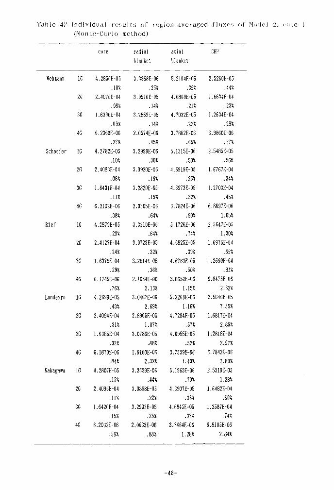
rah I G 42 Individual r e su l t s oï region-averaged fluxes of Model 2, ease(Monte-Carlo method)
Wchmann
Schaefer
Rief
Landeyro
Magawa
1G
2G
3G
4G
1G
2G
3G
4G
1G
2G
3G
4G
1G
2G
3G
4G
IG
2G
3G
4G
core
4.2856E-05. 10%
2.4070E-04.08*
1.6396E-04.09%
6.2360E-06.27%
4.2782E-05.10%
2.4083E-04.08$
1.6431E-04.in
6.2192E-0G.38%
4.2879E-05.29%
2.4127E-04.24%
1.6379E-04.29*
6J745E-06.76%
4.2699E-05.43%
2.4094E-04.31%
1.6385E-04.32%
6.1870E-06.84*
4.2807E-0S.15%
2-4096E-04.11%
1.6420E-04.15%
6.2032E-06.59%
radialblanket
3.3368E-06.25%
3.0916E-05.14%
3.2869E-05.14%
2.0574E-06.45%
3.2999E-06.30%
3.0920E-05.19*
3.2820E-05.19%
2.0305E-06
.64%3.3210E-06
.64%3.0723E-05
.32%3.2614E-05
.36*2.1054E-06
2.13%3.0467E-06
2.69%2.8905E-05
1.07*3.0786E-05
.88*1.9160E-0';
2.32*3.3539E-06
.44%3.0898E-05
.22%3.2933E-05
.25%2.0633E-06
.88*
axialblanket
5.2104E-06
.39*4.6860E-05
.21*4.7032E-05
.22%3.7802E-06
.65%5.1315E-06
.50*4.G919E-05
.25*4.6973E-05
.32%3.7824E-06
.90%5.1726E-06
.74%4.6825E-05
.39%4.6763E-05
.50%3.6652E-06
1.15*5.2269E-06
1.16%4.7284E-05
.57*4.6955E-05
.52*3.7539E-06
1.43%5.1963E-06
.70%4.6907E-05
.36%4.6845E-05
.37*3.7464E-06
1.28*
CRP
2.5260E-05.44*
1.6634E-04.23*
1.2634E-04.29%
6.9860E-06.17%
2.5485E-05.56%
1.G767E-04.34*
1.2703E-04.45%
6.8697E-061.65*
2.5647E-051.30%
1.6975E-04.69*
1.2690E-04.81%
6.8475E-062.62%
2.5646E-057.59%
1.6817E-042.89%
1.28I8E-042.97%
6.7842E-067.89*
2.5319E-051.28%
1.6482E-04.60%
1.2587E-04.74%
6.8105E-062.84*
- 4 8 -

Table 43 Individual results of region-averaged fluxes of Model 2, ease 1(Pn method)
Fletcher 1G2G3G4G
core
4.2370E-052.3926E-041.6679E-046.2855E-06
radialblanket
3.5595E-063.5354E-054.02G1E-052.6785E-05
axialblanket
5.4492E-065.3696E-055.7551E-055.0063E-06
CRP
2.5130E-051.6795E-041.3187E-047.9182E-06
Table 44 Individual results of region-averaged fluxes of Model 2, case 1(Sn method)
Buckel 1G2G3G4G
Lee 1G2G3G4G
Alcouffe 1G2G3G4G
Yaroslavzeva 1G2G3G4G
Yamamoto 1G2G3G4G
Takeda 1G2G3G4G
core
4.2809E-052.4065E-041.6403E-046.2105E-06
4.2821E-052.4099E-041.6399E-046.2060E-064.2816E-052.4068E-041.6405E-046.2117E-064.2808E-052.4064E-041.6411E-046.2169E-064.2817E-052.4071E-041.6408E-046.2120E-064.2812E-052.4067E-041.G404E-046.2107E-06
radialblanket
3.3531E-063.1195E-053.3074E-052.0562E-063.3494E-063.1199E-053.3074E-052.0562E-063.3488E-063.1187E-053.3077E-052.0576E-063.3498E-063.1197E-053.3162E-052.0655E-063.3477E-063.1185E-053.3078E-052.0570E-063.3476E-063.1187E-053.3079E-052.0570E-06
axialblanket
S.2136E-064.7403E-054.7289E-053.74G8E-065.2123E-064.7412E-054.7292E-053.7470E-065.2092E-064.7387E-054.7294E-053.7484E-065.2206E-064.7459E-054.7480E-053.7685E-065.2093E-064.7387E-054.7295E-053.7485E-065.2097E-064.7393E-054.7296E-053.7486E-06
CRP
2.5553E-051.6697E-041.2675E-046.9127E-062.5562E-051.6700E-041.2670E-046.9108E-062.55S8E-051.6693E-041.2676E-046.9175E-062.5579E-051.6697E-041.2688E-046.9478E-062.5553E-051.6695E-041.2677E-046.9169E-062.5551E-051.6694E-041.2674E-046.9157E-06
- 4 9 -

Table 45 Individual results of region-averaged fluxes of Model 2, case 1(Other methods)
Collins (Nodal methodNDT 1G
2G3G4G
NTT 1G2G3G4G
core
)4.2456E-052.4006E-041.6407E-04G.2262E-064.2766E-052.4059E-041.6406E-04G.2147E-06
Ait Abderrahim (Synthesis method)1G2G3G4G
NDT : Nodal DiffusionNTT : Nodal Transport
4.0369E-052.3970E-041.7128E-046.5905E-06
TheoryTheory
radialblanket
3.6576E-063.1971E-053.3490E-052.0755E-063.4022E-063.1169E-053.3012E-052.0559E-06
3.2489E-063.1736E-053.4866E-052.2119E-06
axialblanket
5.7219E-064.8594E-054.7806E-053.7736E-065.2868E-064.7367E-054.7206E-053.7529E-06
4.9696E-064.7186E-054.8817E-053.8902E-06
CRP
2.7095E-051.6791E-041.2638E-046.7763E-062.5584E-051.6646E-041.2653E-04C.9475E-06
2.5241E-051.7317E-041.3650E-047.3544E-06
- 5 0 -

l'ablc 46 Individual results of region-averaged fluxes of Model 2, case 2(Monte-Carlo method)
Wehmann
Schaefer
Rief
Landeyro
Nakagawa
1G
2G
3G
4G
1G
2G
3G
4G
1G
2G
3G
4G
1G
2G
3G
4G
1G
2G
3G
4G
core
4.3516E-05.10%
2.4176E-04.08*
1.6187E-04.09*
B.0436E-06.28%
4.3470E-05.10*
2.4180E-04.09*
1.6207E-04.13*
6.0304E-06.41*
4.3478E-05.24*
2.4189E-04.21*
1.G203E-04.23*
6.0369E-06.60*
4.3504E-0S.46*
2.4155E-04.36*
1.6149E-04.32*
6.0737E-06.90*
4.3428E-05.15*
2.4153E-04.10*
1.6241E-04.15*
6.0565E-06.53*
radialblanket
3.3180E-06.25*
3.0508E-05.14*
3.2239E-05.15*
2.0196E-06.46*
3.3179E-06.33*
3.0365E-05.18*
3.2070E-05.20*
1.9749E-06.66*
3.3333E-06.53*
3.0456E-05.30*
3.2030E-05.31*
2.0029E-06.83*
3.1025E-062.54*
2.8586E-051.02*
3.0275E-05.90*
1.8828E-062.58*
3.3233E-06.45*
3.0470E-05.21*
3.2065E-05.25*
2.0015E-06
.m
axialblanket
5.2344E-06.38*
4.6836E-05.21*
4.6184E-05.23*
3.6257E-06.66*
5.1985E-06.48*
4.6788E-05.25*
4.6102E-05.30*
3.6703E-06.84*
5.2216E-06.64*
4.6888E-05.35*
4.6085E-05.38*
3.6044E-061.04*
5.1761E-061.23*
4.6152E-05.53*
4.6402E-05.54*
3.6373E-061.46*
5.2382E-06.70*
4.6847E-05.36*
4.6242E-05.38*
3.5505E-061.22*
CRP
2.5823E-05.61*
1.6777E-04.33*
1.2561E-04.41*
6.8304E-041.61*
2.5884E-05.84*
1.6738E-04.47*
1.2578E-04.61*
6.9712E-06
2.29*2.5649E-05
1.21*1.6776E-04
.61*1.2449E-04
.75*6.6635E-06
2.57*2.5896E-05
7.77*1.6451E-04
2.88*1.2489E-04
2.70*6.7440E-06
7.85*2.6290E-05
1.26*1.6877E-04
.63*1.2467E-04
.83*7.0249E-06
3.23*
CR
1.6486E-05.71*
9.0932E-05.36*
5.1472E-05.40*
1.0974E-061.36*
1.6539E-051.01*
9.1032E-05.47*
5.2142E-05.56*
1.1092E-061.85*
1.6703E-051.62*
9.1555E-05.83*
5.1903E-05.85*
1.1229E-062.44*
1.6451E-059.48*
9.0813E-052.97*
5.2261E-052.97*
1.0790E-069.36*
1.69I9E-051.48*
9.1556E-05.70*
5.2444E-05.75*
1.1415E-062.48*
- 5 1 -

Table 47 Individual results of region-averaged fluxes of Model 2, case 2(Pn method)
core radial axial CRP CRblanket blanket
Fletcher 1G2G3G4G
4.2725E-052.3884E-041.6194E-046.0935E-06
3.5250E-063.4677E-053.9126E-052.S970E-0G
1.1977E-045.3188E-055.6267E-054.8485E-06
2.5396E-051.6799E-051.2961E-057.72Û9E-06
3.503GE-051.8825E-041.0502E-042.1114E-0G
Table 48 Individual results of region-averaged fluxes of Model 2, case 2
(Sn method)
SnBuckel
Lee
Alcouffe
Yaroslavzeva
Yanamoto
Takeda
1G2G3G4G1G2G3G4G1G2G3G4G1G2G3G4G
1G2G3G4G1G2G3G4G
core
4.3457E-052.4164E-041.6198E-046.0321E-064.3478E-052.4176E-041.6195E-04
6.0284E-064.3469E-052.4174E-041.6199E-046.0356E-064.3457E-052.4167E-041.6206E-046.0357E-064.3468E-052.4170E-041.6201E-046.0332E-064.3456E-052.4164E-041.6198E-046.Û320E-06
radialblanket
3.338GE-063.0762E-053.2332E-052.0020E-063.3349E-0G3.0765E-053.2335E-052.0022E-063.3347E-063.0751E-053.2336E-052.0035E-063.3341E-063.0751E-053.2389E-052.0088E-063.3334E-063.0751E-053.2334E-052.0027E-063.3325E-063.0745E-053.2329E-052.0024E-06
axialblanket
5.2773E-064.7339E-054.6558E-053.6437E-065.2716E-064.7349E-054.6566E-053.6440E-065.2736E-064.7336E-054.6565E-053.6505E-065.2810E-064.7378E-054.6688E-053.6599E-065.2735E-064.7325E-054.6562E-053.6453E-065.2725E-064.7320E-054.6559E-053.6450E-06
CPP
2.6037E-051.6799E-041.2507E-046.6808E-062.6049E-051.6809E-D41.2512E-046.6896E-062.6008E-051.6783E-041.2499E-046.6850E-062.5937E-051.6734E-041.2456E-046.6604E-0G
2.6022E-051.6791E-041.2503E-046.6822E-062.6025E-0S1.G796E-041.2508E-046.6848E-06
CR
1.6756E-059.2460E-055.2451E-05
1.1028E-061.6728E-059.2336E-055.23S6E-051.1478E-061.6741E-059.2431E-055.2454E-051.0883E-06I.6779E-059.2733E-055.2643E-051.0887E-061.6737E-059.2392E-055.2425E-051.1026E-061.6721E-059.2287E-055.2366E-051.1012E-06
- 5 2 -

Table 49 Individual results of region-averaged fluxes of Model 2, case 2(Other methods)
core
Collins (Nodal ,. "Mi)NDT 'G
•&
3G4G
NTT IG2G3G4G
4.3124E-052.4104E-041.6199E-046.0417E-064.3417E-052.4158E-041.6202E-046.0301E-06
Ait Abderrahiœ (Synthesis nethod)
1G2G3G4G
4.0586E-052.4060E-041.7036E-046.4812E-06
radialblanket
3.6414E-063.1S32E-053.2741E-052.0203E-063.3879E-063.0740E-053.2271E-052.0007E-06
3.2201E-063.1473E-053.4478E-052.1828E-06
axialblanket
5.7878E-064.8507E-054.7050E-053.G677E-065.3511E-064.7299E-054.6468E-053.6463E-06
5.0115E-064.7463E-054.8779E-053.8776E-06
CRP
2.7579E-051.6873E-041.2448E-046.5387E-062.5960E-051.6676E-041.2430E-046.6650E-06
2.4621E-051.6816E-041.3020E-046.8899E-06
CR
1.8609E-059.6931E-055.4137E-051.1539E-0G1.7191E-059.3279E-055.2752E-051.1395E-06
1.0541E-055.2711E-052.5986E-053.9622E-07
- 5 3 -

Table 50 Individual results of region-averaged fluxes of Model 3, case 1(Monte-Carlo method)
Wehmann
Schaefer
Rief
Landeyro
Nakagawa
1G
2G
3G
4G
1G
2G
3G
4G
1G
2G
3G
4G
1G
2G
3G
4G
1G
2G
3G
4G
core
2.0337E-05.08%
1.I493E-04.05%
8.2784E-05.06%
3.4158E-06.25%
2.0333E-05.10%
1.1503E-04.08%
8.2813E-05.11%
3.3997E-06.38%
2.0426E-051.09%
1.1392E-041.09%
8.1947E-05l.U%
3.4075E-0G1.78%
2.0408E-05.70%
U526E-04.49%
8.2619E-05.48%
3.4013E-061.47%
2.0325E-05.14%
1.1522E-04.09%
8.2753E-05.13%
3.4009E-06.50%
1
1
1
7
1
1
1
7
1
1
1
7
1
1
1
7.
internalblanket
.2682E-05.45%
.1288E-04.26%
-2015E-04.31%
.4406E-06.91%
.2316E-051.71%
-1005E-041.35%
.1648E-041.35%
.4481E-062.86%
.2391E-051.02%
.1032E-04.57%
.1845E-04.51%
.2503E-061.47%
.2387E-05.66%
.1223E-04
.m.1851E-04
.39%.5432E-06
1.18%
1
1
2
1
1
1
2,
1.
1.
1.
2.
I.
1.
1.
2.
1.
radialblanket
.5888E-06.45%
.6672E-05.29%
.1472E-05.29%
.8012E-06.75%
.6715E-062.46%
.7474E-051.57%
.2122E-051.59%
.8677E-063.02%
.5561E-063.43%
.6744E-051.33%
1612E-05.96%
8329E-062.23%
5898E-06.61%
6825E-05.34%
1582E-05.35%
7854E-06.93%
2
3
3
3
2
3
3
3
2
2,
3,
3.
2.
3.
3.
3.
2.
3.
3.
3.
axialblanket
.9519E-06.34%
.0042E-05.18%
.5361E-05.19%
.7495E-06.46%
.9332E-06.39%
.0190E-05.21%
.5545E-05.24%
.7477E-06.65%
.9411E-061.52%
.9990E-051.16%
.5250E-051.26%
.7606E-061.80%
9516E-061.01%
0164E-05.49%
5289E-05.44%
7491E-06.99%
9191E-06.60%
0148E-05.31%
5358E-05.34%
7665E-06.83%
CRP
1.2214E-05.27%
8.6232E-05.14%
7.4894E-05.17%
5.2953E-06.58%
1.2293E-05.37%
8.6658E-05.21%
7.5453E-05.23%
5.3152E-06.83%
1.3147E-053.14%
9.2048E-051.57%
7.9808E-051.57%
5.5307E-063.88%
1.3482E-058.67%
9.3054E-052.37%
7.9089E-051.31%
5.5J31E-064.27%
1.2160E-05.53%
8.5976E-05.26%
7.5124E-05.31%
5.3233E-061.05%
CR
1.2143E-05.60%
6.7910E-05.30%
3.9733E-05.33%
8.6536E-071.12%
1.2262E-05.82%
6.7618E-05.43%
3.9740E-05.47%
8.7718E-071.53%
8.7141E-066.33%
5.0708E-052.79%
3.3626E-052.91%
1.7055E-067.67%
1.2319E-055.34%
6.7769E-052.28%
3.9406E-052.14%
8.2001E-078.00%
1.I923E-051.25%
6.7545E-05.57%
3.9477E-05.72*
8.5791E-072.23%
- 5 4 -

Table 51 Individual results of region-averaged fluxes of Model 3, case 1(Pn method)
core internalblanket
radialblanket
axialblanket
CRP CR
Fletcher 1G2G3G4G
2.1.8.3.
0391E-051513E-042809E-054015E-06
1117
.1947E-05
.0971E-04
.1888E-04
.5803E-0G
1121
.5541E-06
.6582E-05
.1690E-05
.8549E-06
2.8G87E-063.0770E-053.7543E-054.1841E-06
1975
.3244E-05
.2081E-05
.7G26E-05
.5562E-06
1.2624E-056.8328E-057.9238E-058.3664E-07
Table 52 Individual results of region-averaged fluxes of Model 3, case 1(Sn method)
SnBuckel
Lee
Yamamoto
Takeda
Yaroslavzeva
Alcouffe
1G2G3G4G1G2G3G4G1G2G3G4G1G2G3G4G1G2G3G4G1G2G3G4G
core
2.0370E-051.1491E-048.2641E-053.4001E-062.0381E-051.1499E-048.2647E-053.3990E-062.0378E-051.1497E-048.2674E-053.4012E-062.0380E-051.1498E-048.2684E-053.4015E-062.0376E-051.1492E-048.2618E-053.3950E-062.0400E-051.1503E-048.2608E-053.3934E-06
internalblanket
1.261BE-051.1270E-041.1967E-047.4370E-061.2592E-051.1255E-041.1950E-047.4264E-061.2593E-051.1256E-041.1957E-047.4323E-061.2593E-051.1257E-041.1958E-047.4325E-06
1.2622E-051.1276E-041.1975E-047.4501E-06
radialblanket
1.6069E-061.6792E-052.1585E-051.8070E-061.6076E-061.6812E-052.1633E-051.8142E-061.6060E-061.6795E-052.1590E-051.8074E-061.6065E-061.6798E-052.1590E-051.8059E-06
1.6108E-061.6832E-052.1622E-051.8091E-06
axialblanket
2.9688E-063.0325E-053.5572E-053.7750E-062.9639E-063.0304E-053.5548E-053.7746E-062.9637E-063.0301E-053.555GE-053.7737E-062.9637E-063.0303E-053.5558E-053.7741E-062.9394E-063.0033E-053.5197E-053.7331E-062.9367E-062.9792E-053.4512E-053.6025E-06
CRP
1.2286E-058.6503E-057.5041E-055.2820E-061.2278E-058.G462E-057.4969E-055.2790E-061.2278E-058.6447E-057.5007E-055.2816E-061.2278E-058.6466E-057.5015E-055.2821E-061.2100E-058.5122E-057.3600E-055.1688E-061.3523E-059.4343E-058.0966E-055.5393E-06
CR
1.2367E-056.8653E-054.0168E-058.5711E-071.2341E-056.8585E-054.0H2E-058.5588E-071.2348E-056.8629E-054.0159E-058.5700E-071.2344E-056.8605E-054.0147E-058.5668E-071.2337E-056.8457E-054.0000E-058.4380E-078.1578E-064.6970E-052.8344E-056.2860E-07
- 5 5 -

Table 53 Individual results of region-averaged fluxes of Model 3, case 1(Other methods)
CollinsNDT
NTT
(Nodal1G2G3G4G1G2G3G4G
core
eethod)2.0115E-051.1456E-048.2830E-053.4165E-062.0336E-051.1490E-048.2713E-053.4001E-06
internalblanket
1.3966E-051.1596E-041.2119E-047.4782E-061.2802E-051.1296E-041.19G8E-047.4302E-06
radialblanket
1.7419E-061.7230E-052.1886E-051.8209E-061.6391E-061.6829E-052.1524E-051.7929E-06
axialblanket
3.2283E-063.1081E-053.6036E-053.8115E-062.9909E-063.0320E-053.5528E-053.7G86E-06
CRP
1.3042E-058.7301E-057.5202E-055.2287E-061.2304E-058.6401E-057.5019E-055.2973E-06
CR
1.3666E-057.1719E-054.1396E-058.9797E-071.2666E-056.9125E-054.0361E-058.8696E-07
- 5 6 -

Table 54 Individual results of region-averaged fluxes of Model 3, case 2(Monte-Carlo method)
Wehmann
Schaefer
Landeyro
Nakagawa
1G
2G
3G
4G
1G
2G
3G
4G
1G
2G
3G
4G
1G
2G
3G
4G
core
1.9871E-05.08%
1.1430E-04.0551
8.4536E-05.06%
3.5502E-06.25%
1.9825E-05.10%
1.1446E-04.08%
8.4592E-05.10%
3.5550E-06.35%
1.9926E-05.80%
1.1452E-04.52%
8.4303E-05.53%
3.5366E-061.44%
1.9894E-05.16%
1.1462E-04.10%
8.4317E-05.14%
3.5207E-06.50%
internalblanket
1.2210E-05.41%
1.1257E-04.28%
1.2280E-04.30%
7.8018E-06.88%
1.2282E-051.04%
1.1232E-04.56%
1.2152E-04.49%
7.8277E-061.37%
1.2392E-05.61%
1.1322E-04.39%
1.2232E-04.35%
7.7405E-061.24%
radialblanket
1.52I1E-06.48%
1.6191E-05.30%
2.0985E-05.28%
1.7691E-06.69%
1.5649E-063.33%
1.6269E-051.25%
2.1076E-05.98%
1.7768E-062.16%
1.5363E-06.68%
1.6123E-05.38%
2.1004E-05.40%
1.7794E-06.96%
axialblanket
2.8903E-06.34%
2.9846E-05.18%
3.5694E-05.19%
3.8334E-06.46%
2.8645E-06.43%
2.9851E-05.23%
3.5725E-05.25%
3.8468E-06.67%
2.8571E-061.00%
2.9980E-05.50%
3.5536E-05.41%
3.7954E-06.94%
2.8776E-06.58%
2.9986E-05.32%
3.5687E-05.35%
3.7798E-06.90%
CRP
1.2514E-05.24%
8.8688E-05.12%
7.7475E-05.15%
5.3386E-06.53%
I.2535E-05.32%
8.9100E-05.17%
7.7299E-05.23%
5.3666E-06.75%
1.2472E-059.74%
8.8720E-052.40%
7.7347E-051.81%
5.3234E-064.30%
1.2583E-051.61%
8.9118E-05.57%
7.7155E-05.65%
5.3341E-061.93%
- 5 7 -

Table 55 Individual results of region-averaged fluxes of Model 3, case 2(Pn method)
Fletcher 1G2G3G4G
core
1.9932E-051.1465E-048.4426E-053.5258E-06
internalblanket
1.1774E-051.I04IE-041.2213E-047.890GE-06
radialblanket
1.4835E-061.6070E-052.1299E-051.8178E-06
axialblanket
2.8004E-063.0601E-053.7848E-054.2348E-06
1.9.8.G.
CRP
2499E-050536E-051381E-051031E-06
Table 56 Individual results of region-averaged fluxes of Model 3, case 2(Sn method)
Buckel 1G2G3G4G
Lee IG2G3G4G
Yamauoto 1G2G3G4G
Takeda 1G2G3G4G
Yaroslavzeva 1G2G3G4G
Alcouffe 1G2G3G4G
core
1.9858E-051.1432E-048.4472E-053.5433E-061.9885E-05I.1444E-048.4389E-053.5361E-061.9867E-051.1438E-048.4503E-053.5442E-061.9872E-051.1441E-048.4S29E-0S3.5452E-0G1.9857E-051.1432E-048.4513E-053.5426E-061.9865E-051.1438E-048.4507E-053.5444E-06
internalblanket
1.2419E-051.1349E-041.2348E-047.8079E-061.2333E-05
1.1267E-041.2227E-047.7202E-061.2390E-0S
1.1331E-041.2328E-047.7961E-061.2393E-051.1335E-041.2333E-047.7995E-06
1.2388E-051.1330E-041.2327E-047.7958E-06
11
21112111211121.
1.1.2.1.
radialblanket
.5205E-06
.6170E-05
.0996E-05
.7624E-06
.5406E-06
.6398E-05
.1418E-05
.8087E-06
.5213E-06
.6186E-05
.1022E-05
.7644E-06
.5216E-06
.6189E-05
.1020E-05
.7626E-06
.5218E-0G6192E-051032E-057662E-06
2333233323332333223.3,2,3.3.3.
axialblanket
.8893E-06
.0109E-05
.5894E-05
.8332E-06
.8787E-06
.0003E-05
.5772E-05
.8302E-0G
.8836E-06
.0079E-05
.5869E-05
.8309E-06
.8844E-06
.0089E-05
.5879E-05
.8322E-06
.8631E-06
.9830E-05
.5546E-05
.7925E-06
.8831E-06
.0073E-05,586GE-058329E-06
CRP
1.2614E-058.9258E-057.7633E-0S5.3233E-061.25G1E-058.8834E-057.7057E-055.2833E-0G1.2603E-058.9199E-057.7573E-055.3210E-06
1.2606E-058.9228E-057.7600E-055.3230E-061.2492E-058.8341E-057.6649E-055.2455E-061.2637E-058.9872E-057.8747E-055.4474E-06
- 5 8 -

Table 57 Individual results of region-averaged fluxes of Model 3, case 2(Other methods)
CollinsNDT
NTT
(Nodal1G
203G4G1G2G3G4G
core
method)1.9G0OE-05
1.1398E-048.4679E-053.5646E-061.9825E-051.1430E-048.4534E-053.5481E-06
internalblanket
1.37S0E-05
1.1676E-041.2499E-047.8527E-061.2609E-051.1377E-041.2346E-047.8077E-06
11
211121
radialblanket
.6464E-06
.6581E-05
.1283E-05
.7750E-0G
.5534E-06
.6217E-05
.0952E-05
.7495E-06
axialblanket
3.1427E-063.0868E-053.6368E-053.871IE-OS2.9106E-06
3.0111E-053.S856E-053.8289E-06
CRP
1.3370E-058.9978E-057.7736E-055.2634E-061.2641E-058.9197E-057.7653E-055.3470E-06
- 5 9 -

Table 58 Individual results of region-averaged fluxes of Model 3, case 3(Monte-Carlo method)
Wehnann
Schaefer
Landeyro
Nakagawa
1G
2G
3G
4G
16
2G
3G
4G
1G
2G
3G
4G
1G
2G
3G
4G
core
1.9026E-05
.08*
1.1024E-04
.055i
8.0192E-05
.06*
3.2002E-06
.25%
1.9033E-05
.11%
1.1021E-04
.0835
8.0203E-05
.11%
3.2013E-06
.40%
1.9012E-05
.79*
1.1029E-04
.51%
7.9762E-05
.49%
3.2001E-06
1.40%
1.9058E-05
.15%
U042E-04
.10%
8.0090E-05
.14%
3.1725E-06
.47%
internal
blanket
1.1865E-05
.46%
1.0818E-04
.28%
1.1G52E-04
.30%
7.0597E-06
.98%
1.1842E-05
1.08%
1.0824E-04
.56%
1.16S6E-04
.49%
6.8733E-06
1.31%
1.1903E-05
.60%
1.0885E-04
.40%
1.1717E-04
.40%
7.1613E-06
1.26%
radial
blanket
1.3748E-06
.48%
1.4752E-05
.28%
1.9204E-05
.30%
1.6128E-06
.75%
1.3498E-06
3.11%
1.4S44E-05
1.37%
1.9003E-05
1.02%
1.6084E-06
2.33%
1.3675E-06
.64%
1.4614E-05
.39%
1.9000E-05
.39%
1.6239E-06
.96%
axial
blanket
2.7286E-06
.34%
2.8398E-05
.18%
3.3534E-05
.19%
3.5022E-06
.47%
2.7211E-06
.42%
2.8342E-05
.24%
3.3609E-05
.27%
3.5216E-06
.67%
2.7965E-06
•1.04%
2.8739E-05
.47%
3.4038E-05
.43%
3.5615E-06
.99%
2.7163E-06
.60%
2.8416E-05
.35%
3.3624E-05
.35%
3.5258E-06
.84%
- 6 0 -

Table 59 Individual results of region-averaged fluxes of Model 3, case 3(Pn method)
Fletcher 1G2G3G4G
core
1.9106E-051.1046E-048.0112E-043.1694E-06
internalblanket
radialblanket
axialblanket
2.6435E-062.8839E-053.5362E-053.8573E-06
Table 60 Individual results of region-averaged fluxes of Model 3, case 3(Sn method)
Buckel 1G2G3G4G
Lee 1G2G3G4G
Yaiamoto 1G2G3G4G
Takeda 1G2G3G4G
YarosIavzevaIG2G3G4G
Alcouffe 1G2G3G4G
core
1.9038E-051.1017E-048.0140E-053.1865E-061.9063E-051.1028E-048.0060E-053.1813E-061.9047E-051.1023E-048.0174E-053.1876E-06
1.9055E-051.1028E-048.0210E-053.1890E-061.9037E-051.1017E-048.0183E-053.1865E-061.8954E-051.0982E-048.0006E-0S3.1964E-06
1117111611i.
171117
111G
internalblanket
-1955E-ns.0890E-04.1721E-04.0762E-06.1865E-05.0799E-04.1593E-04.9901E-06.1927E-05.0869E-04.1698E-04.0628E-06.1933E-05.0874E-04.1704E-04.0663E-06
.1030E-05
.0050E-04
.0811E-04
.5342E-0B
1111111111111111
111,1,
radialblanket
.3688E-06
.4728E-05
.9191E-05
.6107E-06
.3906E-06
.4979E-05
.9657E-05
.6605E-06
.3702E-06
.4754E-05
.9228E-05
.6138E-06
.3708E-06
.4758E-05
.9230E-05
.6125E-06
.3711E-06
.4764E-05
.9245E-05
.G160E-06
22332233223322,3,3,2.2.3,3.2.2.3.3.
axialblanket
.7368E-06
.8516E-05
.3758E-0S
.5258E-06
.7255E-06
.8400E-05
.3637E-05
.5255E-06
.7314E-06
.8486E-05
.3730E-05
.5231E-06
.7326E-06
.8499E-05
.3746E-05
.5248E-06
.7096E-068213E-05.3403E-05.4882E-0G7244E-068414E-053G53E-055169E-06
- 6 1 -

Table 61 Individual results of region-averaged fluxes of Model 3, case 3(Other methods)
Collins (NodalNDT 1G
2G3G4G
NTT 1G2G3G4G
Ait Abderrahini1G2G3G4G
core
method)1.8826E-051.0989E-048.0313E-053.2039E-061 9007E-051.1017E-048.0215E-053.1913E-06
(Synthesis method)1.8530E-051.0458E-047.7395E-053.2295E-06
internalblanket
1.3130E-05LlieOE-04
1.1848E-047.1161E-061.2097E-051.0901E-041.I713E-047.0760E-06
4.5322E-064.3552E-055.4533E-053.8575E-06
radialblanket
1.4744E-061.5050E-05
1.9394E-051.6173E-061.3955E-061.4753E-051.9129E-051.5970E-06
2.7072E-062.8030E-053.6439E-053.1295E-06
axialblanket
2.9509E-062.9080E-Û53.4095E-053.5531E-062.7486E-062.8450E-053.3663E-053.5173E-06
2.3309E-062.3692E-052.9089E-053.2220E-06
- 6 2 -

Table 62 Individual results of region-averaged fluxes of Model 4, case 1(Monte-Carlo method)
Nakagawa 1G
2G
3G
4G
Wehœann 1G
2G
3G
4G
1
1
3
3
testzone
1.360E-04.80*
1.103E-04.60%
3.099E-05.56%
3.873E-06.87%
.3497E-04.11%
.0847E-04. 14%
.0723E-04.26%
.8755E-06.51%
axialblanket
3.532E-05.70%
5.010E-05.57%
2.590E-05.75%
1.192E-05.94%
3.5233E-05.25%
4.9748E-05.25%
2.6287E-05.39%
1.2875E-05.34%
driver withModerator
6.493E-05.34%
4.996E-05.22%
2.826E-05.22%
1.446E-05.26%
6.3294E-05.09%
4.9998E-05.09%
2.8204E-05.11%
1.4491E-05.12%
5
5
2
1
CRP
.2497E-05.11%
.0666E-05.12%
.2637E-05.20%
.0366E-05.34%
Table 63 Individual results of region-averaged fluxes of Model 4, case 1(Pn method)
Fletcher 1G2G3G4G
testzone
1.3246E-041.0884E-043.1356E-053.9845E-06
axialblanket
3.8626E-055.3507E-052.7845E-051.2776E-05
driver withloderator
6.3676E-054.8661E-052.7724E-051.4261E-05
CRP
5.3900E-055.1974E-052.3443E-051.1151E-05
- 6 3 -

Table 64 Individual results of region-averaged fluxes of Model 4, case 1(Sn method)
Takeda IG2G3G4G
testzone
1.3435E-051.0791E-043.0289E-053.2917E-06
axialblanket
3.5410E-054.9618E-052.5893E-051.1649E-05
driver withmoderator
6.6393E-055.1327E-052.8424E-051.4341E-05
CRP
5.4226E-055.1474E-052.2143E-059.2927E-06
Table 65 Individual results of region-averaged fluxes of Model 4, case 1(Other methods)
WagnerNT 20
(Nodal1G2G3G4G
testzone
method)1.3317E-041.0741E-043.0910E-053.9903E-06
axialblanket
3.5860E-054.9930E-052.6255E-051.2073E-05
driver withmoderator
6.5622E-055.0333E-052.8358E-051.4532E-05
CRP
5.2673E-055.0610E-052.2703E-051.0527E-05
NT : Nodal Transport20 : Nuuber of axial layers
- 6 4 -

Table 66 Individual results of region-averaged fluxes of Model 4, case 2(Monte-Carlo method)
test axial driver with CRP CRzone blanket moderator
Nakagawa 1G
2G
3G
4G
Wehmann 1G
2G
3G
4G
1.491Ë-04.23%
1.131E-04.22%
2.651E-05.52%
2.477E-061.26%
1.4648E-04.11%
1.1227E-04.14%
2.6574E-05.27%
2.4498E-06.36%
3.683E-05.44%
4.876E-05.39%
2.250E-05.71%
8.547E-061.29%
3.7218E-05.25%
4.8757E-05.25%
2.2307E-05.40%
8.7007E-06.67%
7.001E-05.14%
5.108E-05.44%
2.774E-05.23%
1.399E-05.27%
7.0408E-05.09%
5.1358E-05.09%
2.7716E-05.11%
1.3943E-05.13%
1.1866E-04.14%
1.0031E-04.16%
3.6997E-05.27%
1.1076E-05.48%
4.4354E-05.17%
3.5773E-05.18%
7.7894E-06.32%
4.8143E-07.43%
Table 67 Individual results of region-averaged fluxes of Model 4, case 2(Pn method)
Fletcher IG2G3G4G
testzone
1.4619E-041.1202E-042.6725E-052.6008E-06
axialblanket
4.0153E-055.1692E-052.3587E-059.2026E-06
driver withmoderator
6.9230E-055.0327E-052.7600E-051.3969E-05
CRP
1.1947E-049.9713E-053.7225E-051.1472E-05
CR
4.5836E-053.6277E-051.2536E-053.8632E-06
- 6 5 -
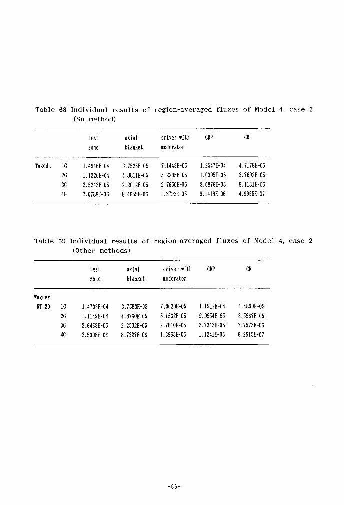
Table 68 Individual results of region-averaged fluxes of Model 4, case 2(Sn method)
Takeda 1G2G3G4G
testzone
1.4946E-041.1226E-Ù42.5243E-052.0788E-06
axialblanket
3.7525E-054.8811E-052.2012E-058.4655E-06
driver withnoderator
7.1443E-055.2295E-052.7650E-051.3793E-05
CRP
1.2547E-041.0395E-053.6876E-059.1418E-06
CR
4.7178E-053.7692E-058.1131E-064.9955E-07
Table 69 Individual results of region-averaged fluxes of Model 4, case 2(Other methods)
WagnerNT 20 1G
2G3G4G
testzone
1.4733E-041.1149E-042.6463E-052.5308E-06
axialblanket
3.7583E-054.8760E-052.2502E-058.7327E-06
driver withmoderator
7.0620E-055.1532E-052.7810E-051.3965E-05
CRP
1.1912E-049.9954E-053.7343E-051.1241E-05
CR
4.4890E-053.5967E-057.7973E-066.2915E-07
- 6 6 -

Table 70 Individual results of region-averaged fluxes of Model 4, case 3
(Monte-Carlo method)
Nakagawa 1G
2G
3G
4G
Wehmann 1G
2G
3G
4G
testzone
1.672E-04.92*
1.177E-04.77*
2.188E-05.87%
1.174E-061.73%
1.49G3E-04.in
1.1674E-04.14%
2.1816E-05.31%
1.1658E-06.42%
axialblanket
4.103E-05.72%
5.243E-05.66%
2.380E-05.78%
9.733E-051.23%
4.0616E-05.25%
5.1744E-05.25%
2.3588E-05.40%
9.7430E-06.43%
driver withuoderator
7.454E-05.41%
5.171E-05.32%
2.698E-05.36%
1.340E-05.40%
7.5020E-05.10%
5.1923E-05.10%
2.6956E-05.12%
1.3390E-05.14%
CR
9.586E-05.28%
6.962E-05.34%
1.344E-05.47%
9.728E-07.95%
9.5412E-05.11%
6.9278E-05.12%
1.3436E-05.23%
9.4854E-07.44%
Table 71 Individual results of region-averaged fluxes of Model 4, case 3(Pn method)
Fletcher 1G2G3G4G
testzone
1.6004E-041.1445E-042.1475E-051.2197E-07
axialblanket
4.3773E-055.5105E-052.4826E-051.0372E-05
driver withaoderator
7.4091E-055.1229E-052.7126E-051.3616E-05
CR
9.6475E-056.8633E-051.2895E-058.2098E-07
- 6 7 -
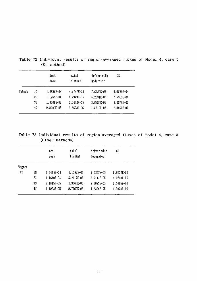
Table 72 Individual results of region-averaged fluxes of Model 4, case 3(Sn method)
Takeda 1G2G3G4G
testzone
1.6885E-041.1766E-041.9566E-059.8209E-05
axialblanket
4.1747E-055.2949E-052.3442E-059.5603E-06
driver withmoderator
7.6295E-05S.2631E-052.6580E-051.3210E-05
CR
1.0559E-047.5813E-051.4578E-057.8467E-07
Table 73 Individual results of region-averaged fluxes of Model 4, case 3(Other methods)
WagnerNT 1G
2G3G4G
testzone
1.6465E-041.1640E-042.1815E-051.1923E-05
axialblanket
4.1097E-055.2117E-052.3668E-059.7162E-06
driver withmoderator
7.5255E-055.2147E-052.7023E-051.3396E-05
CR
9.6537E-056.9708E-051.3615E-041.0023E-06
- 6 8 -

mesh
d i v is ion
1 0
5
.0
.0
( 1 5 )
1 5 . 0
2 5 . 0(cm)
( 1 5 ) ( 5 ) ( 5 ) _ , , , --" R e f l e c t i v e
1 5 . 0 2 0 . 0 / 2 5 . 0 (cm)•> x
R e f l e c t o r
Vacuum
C o n t r o l r o d ( c a s e 2 )
o r V o i d ( e a s e l )
V a c u u m
1/4 core
isesh
d iv is ion
I 0.0
(15)
15.0
(10)
R e f l e c t i v e25.0(cm)
Vacuum
Reflective
> x y
Vacuum
C o n t r o l R o d ( c a s e 2 )
o r V o i d ( e a s e l )
Fig. i Core configuration of Model 1
-69-

Y (cm)
mesh. .division
reflective
(11)
0 Lcorecentei (7)
reflective
35 45 55 70(2) (2) (3)
(7)meshdivisionOO
(4)
20
0v a c u u m
(2) (2 ) (3 )35 45 55 70
meshdivision
(11)
reflective
75
X(cm) (11)
meshdivision
CR : Control rodCRP: Na filled ...
control rod position ( }
130
150
AXIALBLANKET
1CORE
corecenter
CORE
AXIALBLANKET
v a c u
1r•IGRI••
:RP*
u m
RADIAL
BLAMINKET
V
ac
uum
Fig. 2 Core configuration of Model 2 Z(cm)
X(cra)

~ ( 3 1K 5
( 5 )
120
33
35
(6)
core 'center
K \ 1 x•\
r\\
i i
X
X
X
xX
XX
y.
X
XxX
XX
\ J \
\ l \
<
\
\
\
\
\
\\
•;. RADIAREFL
\N[\\
\ Nx
- CRP"-: 1
X| XX i XXV
rah'"CKr
XX
X
X
X
XX
X
X
X
X
X
x!xxV
71
'AX
X
Tfxx|xX
XX
/ •
X xVo-'XlX^.A(xfx
x
XX
X
\
V
X
X
\ ^ \
E
\
X
X
X
\
\
htECTO
A'
DIAL"LANKE
\
X
X
TERNALLANKET,- /••
X X
XX
AXI
X
CX
X
x
y-Y4--X
X
X
Tfx
X
X
X
XX
X
7>x
\
:o
X
X
X
AX
X
XX
X
X
x|x*xCRP»',
x
\\
RE
><
X
X
X
\
\
T
\\
!cX
X
X
X
X
X | X
xlxX I X
X
X
X
X
R17
\z•7
Ay
\\\\
\\\\\
x | \
XX
X
XX
X
XX
7}XIX|X
X
XX
X
XX
XX
f- u
4*A/Ay\\x\\_\
A
X
X
xxxX
\\
\\\\\
/
cxXX
1
/ //
/
\\
/F7
-
AAA
A/
\ j \
\ f \\ [ \v \
\\\x
\ X \
j
1
RP•
7///
—r f -
_j_• EMP
i /
/ /!7V
\ ] \\J\\ ] \
\I\T\
h ^̂
\
/\\\\\\\\\
//\\
y/_
/
7
1 -)—i _T1
t-iz
MA
\//
/'V
\
\J\s.
\
\
\
\
A/\\
\ j \\\\\\
\\
\\\^\^V\\\
/~A777
////
/A\\
i
Uz" R i x
/ /' A/
\i \\ K\ K\\\\\
W
K̂\
\\\\\\\\
\ \
//
\\\\\\\ l
\
y\A7//
-
/,.'////
/ /\\\\\\
////
/
I
rf
/7//
/7/
////A/A/..
V
1
cJ
(6)
35 45
(2)
80
(7)
reflective
(8 )
120 U S 160(c«)
(51 (3)meah -̂division
(en)
meshdivision 90.0
(2)30.0
(5)
55.0
(9)
10.0(2)
0 . 0 ;
A X I A L
A X I A L
C O R E
CR : Control rodCRP: Na filled
control rod position
v a c u u m
I N T E R N A L
R E F L E C T O R
B L A N K E T
C O R E
B L A N K E T
RADIAL
BLANKET
core/0.0 5.0center (1)
35.0 45.0(6) (2)
r e f 1 e c
(7 )•W:ov
RADIAL
REFLECTOR
(8)120.0 145.0 160.0 (cm)
(5) tJÏ mesh d iv i s ion
Fig. 3a Core configuration of Model 3
-71-

transverse az. Ai"
I6C
(cm)
m e s h • 90 Q(2)
80.0
(5)
55.0
(9)
(2)10.0
0.0 < L -'o .o
corecenter
v a c u u m
A X I A L R E F L E C T O R
A X I A L L A N K t T
C O R E
N T E R N A L B L A N K E Tf l e c t i v e
RADIALBLANKET
RADIALREFLECTOR
X
80.0 120.0 145.0 160.0 (cm)(1G) (8) (5) (3) mesh divis ion
Fig. 3b Core config-uration of Model 3
- 7 2 -

\OJ
h d -A d = 7.50 cm
Test Zone
control Rod /Control Rod Follower
Driver Without Moderator
Driver With Moderator
$ § & Reflector Without^s Moderator
# Reflector WithModerator
KNK-1 Reflector
Sodium / Steel Zone
z(cm)
me3h division
\7)
155 0-(2)
145.0(1)
125.0-
(6)
95. Or
(G) A
G5 0-
W
(9)
0.0
10 9 8 7
1
3
6
3
1
1
3
5
3
1
centero
l
2
H
2
1
r
1
2
2
\
axis
1
2
2
1
1
3
5
3
1
1
3
G
3
i
7 3 9 10
Note 1; Steal2; Axial Blanket3; Axial Reflector4i Test Zone
7;Refiector withoutModerator
8;Reflector with Moderator9 jKNK-1 Reflector
5i Driver without Moderator 101 Sodium/S teel6; Driver with Moderator (VACUUM at all outer surfaces'
Fig. 4a Core configuration of Model 4

z(cm)190.00
Withdrawn half-inserted fully inserted
155.00 -
125.00 -
95.00 -
65,00 ~
0.00 -J
c0
•H+J
M0
a
ou+Jcou
'D
•H•aow
CDCD+J
c -o
XIo
o1-1+1ou
XIO
CDCD+-»C/J
Pi
CDCD
COoo
— Core UpperBoundary
Core Midplane
... Core LowerBoundary
Fig. 4b Control rod pattern on Model 4
- 7 4 -

0.984
0.983
0.982-
0.931-
0.98-
0.979-
0.978-
0.977-
0.976-1
0.975'
Model 1case 1
Exact fiC fiC Pnni
34 38
Fig. 5 Average k e f f of Model 1, case 1
XRR D0T3.5
0.964'
Model 1
case 2
0.9638'0.9636-0.9634-0.9632-
0.963-0.9628-0.9626-0.9624-0.9622-
0.962-0.9618-0.9616-
Exac t I1C MC Pn 34 • :-::s-; CCRR DOTS.5
Fig. 6 Average of Model 1, case 2
- 7 5 -
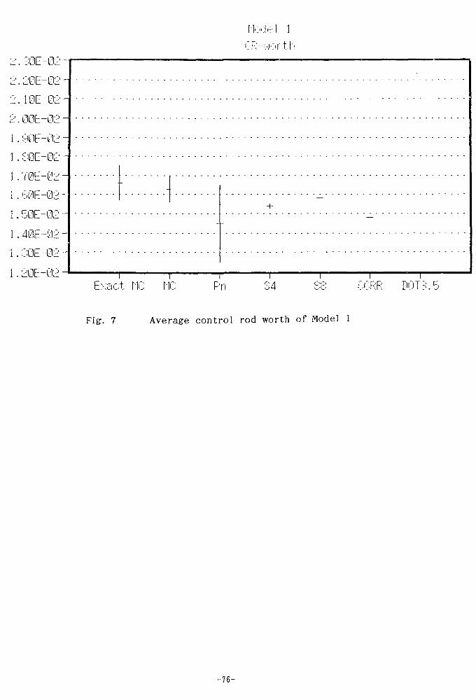
2.20E-02-
2. 10E-02-
2.00E-02
1.90E-02 -
1.&0E-02 -
1. 60
Exact Pni
94 CCRR DÛT3.5
Fig. 7 Average control rod worth of Model 1
-76-

0.9:?
0.979 -
0.978-
0.977
0.976
0.975-
0.974-
0.973-
0.972-
0.971
•+-
Exact
Fig. 8 Average
Pn c ••34r
(•••:":• DIF3D(NTT) CCRR
of Model 2, case 1
0.965
0.964-
0.963-
0.962-
0.961-
0.96
0.959-
0.953
Model 2case 2
0.957-
"+•
Exact MC TIC Pn S4 S8 DIF3D(NTT) CCRR
Fig. 9 Average k e f f of Model 2, case 2
- 7 7 -

CR-worth1.57E-02•
1.56E-02•
1 54E-02
53E-02
51E-02
50E-02•
49E-02•
43E-02•
47E-02•
46E-02•
44E-02•
43E-02•Exact ML
I
Pn S4 DIF3D(NTT) CCRR
Fig. 10 Average control rod worth of Model 2
- 7 8 -

ca be0.97S
0.977
0.976
0.975
0.974
0.973-
0.972 -
0.971 -
0.97-
0.969 -
0.968 -
0.967
• + • •f
Q .-••+ Md1.- '- I ne Pn DIF3D(NTT) CCRR
Fig. 11 Average k p f f of Model 3, case 1eff
Model 3
case 2
.003-
.002
1 H
0.999 -\
0
0
0
yyr H
Exact Pn S4 88 DIF3D(NTT) CCRR
Fig. 12 Average keff of Model 3, case 2
-79-

case
IJe
1.025
1.024 -
1.023 -
a 1.022-
1.021 -
S4 S8 DIF3DCMTT)
Fig. 13 Average keff of Model 3, case 3
3.10E-02-
3.00E-02-
2.90E-02-
2.80E-02-
2.70E-02
Model 3CR-worth
Exact MC MC Pn S4 38 DIF3DCNTT) CCKR
Fig. 14 Average control rod worth of Model 3
- 8 0 -

.11E-02-
.10E-02-
.09E-02•
.0SE-02•
.07E-02
06E-02•
05E-02•
CRP-i.-.iortl
o
2.04E-02-
2.03E-02-
2.02E-02-
2.01E-02-
2.00E-02-
1.99E-02•Exact tic TIC Pn S4 DIFSEKNTT)
Fig. 15 Average control rod position worth of Model 3
-81-

Cri :-.6
9ri-
n
a
. 097
. 096
. 095
.094-
. 093 •
. 092 •
.091 •
1.09 •
.039-
.038-
.037-
. 036 -
.035-
.034-Exact I1C I1C
Fig. 16 Average
Pn HEXNOD(NT) CVEl
of Model 4, case 1
Model 4
gir-.
n
0.994
0.992-
0.99 -
0.983
0.986-
0.934-
0.932-
0.98
0.973-1
0.976
0.974Exact MC MC
i
Pn S3 CHEZHEXMOD(MT) CHE
Fig. 17 Average keff of Model 4, case 2
-82-

0.91 -
0.9-
0.39-
0 .88-
0.87
2.6OE-01
2.50E-01 -
2.40E-01 -
2 .30E-01-
2 .20E-01-
2 .10E-01-
2 .00E-01-
1.90E-01
Model 4case o
• \
Exact fiC 11 Pri SB HEXNOD(NT) CI1EZ
Fig, 18 Average keff of Model 4, case 3
Model 4
CR-worth
Exact I1C NC F:in CO HEXNOD(NT) CMEZ
Fig. 19 Average control rod worth of Model 4
-83-

k e f f
0 . 9 7 7 2
0 . 9 7 7 1
0 . 9 7 7 0
0 . 9 6 2 5
0 . 9 6 2 4
0 . 9 6 2 3
0 . 9 6 2 2
-
-
-
i i i i
rod-c
I 1 i 1
u t
1 1 1 ! 1 1 1 1 1 I 1 1
)
-
-
-
-
-
> .
1 1 1 1
^ - —
l i l t
' ©
1 1 1 1
— .
i i i i
rod-i—
I I I I
n• •
1 1 1 1
—
I I I I
—
I I I I
" — .
| I 1 t
" i
i t i i I I I I
-
-
-
-
0.0 0.2 0.4 0.6Square inverse of mesh interval
0.8 1.0(cm~2)
Fig. 20 Spatial mesh effect on k e f f for rod-ln and rod-outcases of Model 1
-84-

Appendix 1 : "Specifications of calculational benchmark models"
Calculational method
Any calculational methods are acceptable. Not only the direct 3-D treatment such as the
3-D Sn, 3-D nodal transport and Monte-Carlo method, but also the combined use of 1-D and
2-D (XY, Hexagonal, Triangular and RZ) transport calculations can be used.
The following conditions are recommended to use:
1) Flux normalization
The total production of the whole reactor is normalized to unity.
Z/vdrvZ fe(r)<DB(r) = 1g -
2) Isotropic scattering
The Pj scattering effect is included by using the transport cross section instead of total
cross section.
3) Multigroup cross sections
The few-group cross sections are given in order to remove the effect of the difference
between participants.
The cross section 2 (transport cross section), 2 , (scattering cross section), v2,
(production cross section), x (fission spectrum) are used as in the conventional manner, assum-
ing that xg is not space dependent:
Qgrad<Dg(r,Q) + 2,g(r) <Dg(r,Q) = 2 2 s g^ g
4JD g
+ 2 v 2 f ( r) /vdQ*(r ,Q)4*keff «
The absorption cross section satisfies the relation
- 8 5 -

a g 'g g. sg-»g'
which means that (n,2n) or (n,3n) processes are not taken into account.
4) Trie examples of the mesh sizes are given for each calculational model; participants may
take their appropriate angle and space meshes. S4 or Sg quadrature set will be used at Osaka
University (Appendix 2). If possible, it is desirable to calculate the solution extrapolated to fine
mesh and Sinfinj|, solutions.
The convergence criterion (relative difference between successive iterations) used at
Osaka University is as follows;
Inner iteration : AC>/<t> < 5x10~4
Outer iteration : Ak / k < 5x10~5
All participants are requested to supply information on resources used in their computa-
tions, e.g. CPU time, core storage, computer type, etc.. Additional information so as to specify
clearly how their computations were run are also requested. For example, Monte-Carlo submit-
tals should include information on variance reduction techniques used in the Monte-Carlo runs,
and numbers of histories per generation and number of generations.
Calculational model
We consider the following four reactor cores. Participants may choose as many reactor
cores as they wish out of the reactor cores provided.
Model 1 (Small LWR)
This core is similar to Kyoto University Critical Assembly (KUCA). The main features
are as follows:
- 8 6 -

Polyethylene moderated
93 w/o enriched U-Al alloy & natural U metal plates
Average 235U enrichment 9.6 w/o, VM / VF = 1.5
1/8 core dimension : X x Y x Z = 15cm x 15crn x 15cm (Fig. 1)
The mesh size used at Osaka University for reference calculation is lem x lem x lcm.
The control rods are located at core/reflector boundary as shown in Fig. 1.
We consider the following tow cases;
case 1 : The control rod position is empty (void)
case 2 : The control rod is inserted as shown in Fig. 1
It has been found that the control rod worth becomes negative when one utilizes diffu-
sion calculations. Then the transport effect is very strong for control rod worth. The 2-group
cross sections are given in Appendix 2.
Required solutions
a) keff for the two cases, and control rod worth defined by1
k'e£f case 2 keff
case 1
b) Region-averaged fluxes
Two-group fluxes averaged in the core region, reflector region, control rod or void
region.
c) Region-averaged reaction rates
Production and absorption rates in the core and the reflector regions, and the neutron
leakage rates from the two regions in each group.
d) Energy group wise flux distributions
Distributions of mesh-averaged flux for the reference mesh (lcm x lcm x lcm) is appro-
priate. The following distributions are required:
- 8 7 -

1) along X-axis (0.0<X<25.0, 0.0<Y<1.0) on the (0.0<Z<1.0) plane.
2) along Y-axis (0.0<X<1.0, 0.0<Y<25.0) on the (0.0<Z<1.0) plane.
3) along the Z-axis (0.0<X<1.0, 0.0<Y<1.0, 0.0<Z<25.0)
Model 2 (Small FBR)
The core geometry (quarter core) is shown in Fig. 2. The reference mesh size used at
Osaka University is 5cm x 5cm x 5cm.
We consider the cases without control rod (case 1; control rod position is filled with Na)
and with control rod half-inserted, (case 2) The core calculation is performed in 4-groups. The
4-group cross sections and energy group structure are listed in Appendix 4.
Required solutions
a) ke£f for the two cases ; control rod worth
b) Region-averaged reaction rates
Production, absorption and leakage rates in the core, radial blanket, axial blanket, Na
filled control rod positions and control rod regions in each group.
c) 238U capture, 238U fission and 239Pu fission rate distributions along X and Y axes at the core
midplane rates for the reference mesh size (5cm x 5cm x 5cm) are appropriate, i.e., (0.0<X<70.0,
0.0<Y<5.0) for X-axis, and (0.0<X<5.0, 0.0<Y<70.0) for Y-axis. 238U capture, 238U fission and
239Pu fission macroscopic cross sections are listed below.
Energy Group
1234
238U capture
1.184E-4*1.076E-33.858E-39.221E-3
238U fission
3.101E-32.418E-55.354E-74.543E-6
* : Read asunit =
239Pu fission
2.192E-31.91/E-32.241E-36.827E-3
1.184xlO"4
cm

d) Region-averaged group wise fluxes for core, axial blanket, radial blanket, Na filled rod posi-
tions and control rod regions.
e) For case 2, radial flux distribution along X-axis on Z = 72.5cm plane near the core midplane.
Distributions of mesh-averaged flux for the reference mesh size (5cm x 5cm x 5cm) are appro-
priate.
Model 3 (Axial ly heterogeneous FBR)
This core has an internal blanket region as in Fig. 3. Furthermore, both center and off-
center control rods will be inserted, so that it is difficult to evaluate the core characteristics by 2 -
D modeling.
The reference mesh size used at Osaka University is 5cm x 5cm x 5cm. 4-group, 1/8
core calculations will be performed. The cross sections are listed in Appendix 3, which is the
same as for the small FBR core, Model 2.
We considered the following three cases:
case 1 : control rods are inserted
case 2 : control rods are withdrawn
case 3 : control rods are replaced with core and/or blanket cells as shown Fig. 3b
Required solutions : all solutions required for the three cases.
a) keff ; control rod worth obtained from case 1 and case 2, and control rod position worth ob-
tained from case 2 and case 3
b) Region-averaged reaction rates
Production, absorption and leakage rates in the core, internal blanket, radial blanket, axial
blanket, Na filled control rod positions and control rod regions.
c) 238U capture, 238U fission and 239Pu fission rate distributions along X-axis and transverse at
- 8 9 -

45° (sec Fig. 3a and 3b) at the Z-plane (0.0<Z<5.0). Mesh-averaged values appropriate, i.e.
(0.0<X<lC0.0, 0<Y<5.0) for X-axis. 238U capture, 238U fission and 239Pu fission macroscopic
cross sections are the same as given for Model 2.
d) Flux distributions along X-axis and transverse at 45° at (0.0<Z<5.0) and (50.0<Z<55.0)
planes.
c) Region-averaged group wise fluxes for core, axial blanket, radial blanket, internal blanket, Na
filled control rod positions and control rod regions.
Model 4 (Small FBR with Hexagonal-Z geometry)
This core model is similar to the KNK-II core proposed by I. Broeders and E. Kiefhaber
of KfK, Germany.® The core is considered of hexagonal subassemblies; cylindrical model is in
general a poor approximation. Furthermore, the transport effect is emphasized due to small size
of the core and the local insertion of control rods. Therefore, a three-dimensional hexagonal-Z
treatment is necessary.
Energy structure and cross sections in four groups listed in Appendix 5.
The core configurations are shown in Fig. 4a.
The control rod patterns are considered as shown in Fig. 4b; control rod withdrawn (case
1), half inserted (case 2) and fully instead (case 3).
Required solutions
a) keff for all cases
b) control rod worth
c) subassembly-averaged production rates at core midplane (95.0<Z<100.0) for all cases
d) Regio-averaged group fluxes for all regions
- 9 0 -
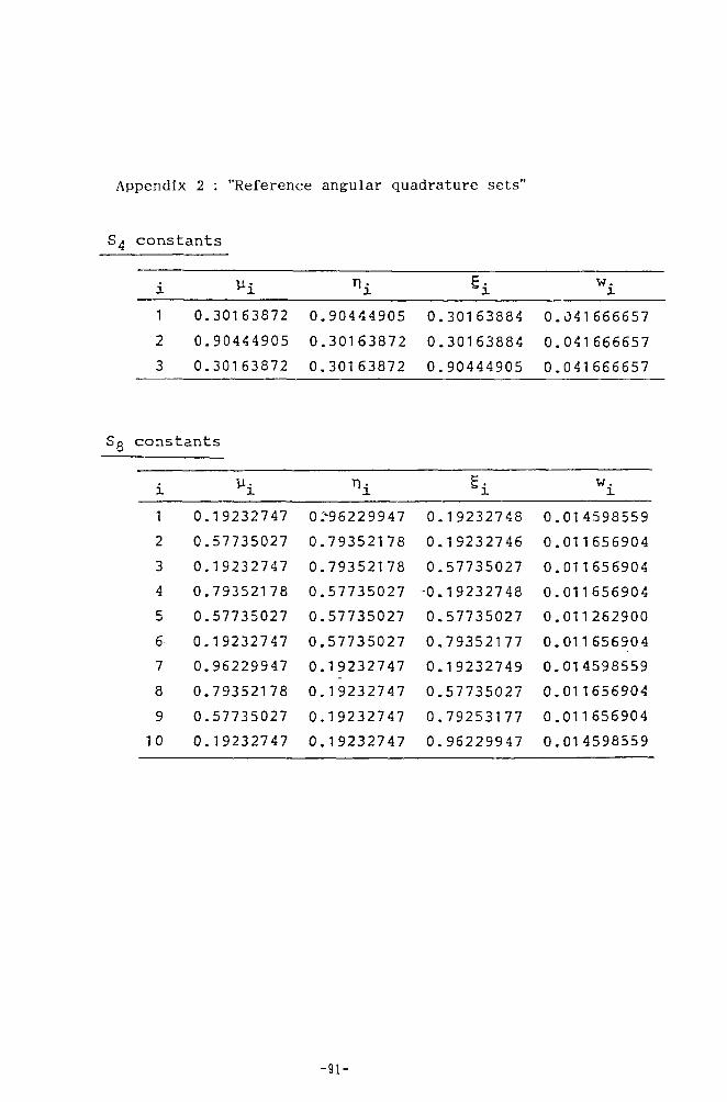
Appendix 2 : "Reference angular quadrature sets"
S.. constants
w.
1
2
3
0.30163872
0.90444905
0.30163872
0.90444905
0.30163872
0.30163872
0.30163884
0.30163884
0.90444905
0.Û41666657
0.041666657
0.041666657
c o n s t a n t s
1
i
1
2
3
4c
6
7
8
9
0
Ui
0.19232747
0.57735027
0.19232747
0.79352178
0.57735027
0.19232747
0.96229947
0.79352178
0.57735027
0.19232747
*i
0J-96229947
0.79352178
0.79352178
0.57735027
0.57735027
0.57735027
0.19232747
0.19232747
0.19232747
0.19232747
£±
0.19232748
0.19232746
0.57735027
-0.19232748
0.57735027
0.79352177
0.19232749
0.57735027
0.79253177
0.96229947
0.01
0.01
0.01
0.01
0.01
0.01
0.01
0.01
0.01
0.01
Wi
4598559
1656904
1656904
1656904
1262900
1656904
4598559
1656904
1656904
4598559
-91-
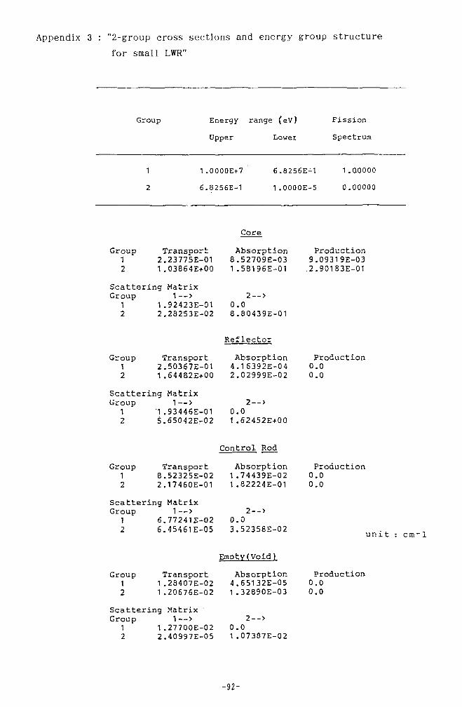
Appendix 3 : "2-group cross sections and energy group structure
for small LWR"
Group Energy range (eV)
Group12
Upper Lower
Fission
Spectrum
1 1.0000E+7 6.8256E-1 1.00000
2 6.8256E-1 1.OOOOE-5 0.00000
Transport2.23775E-011.03864E+00
Scattering MatrixGroup 1-->
1 1.92423E-012 2.28253E-02
Group12
Transport2.50367E-011.644S2E+00
Scattering MatrixGroup 1—>
1 "1.93446E-012 5.65042E-02
Group12
Transport8.52325E-022.17460E-01
Scattering MatrixGroup 1-->
1 6.77241E-022 6.45461E-05
Group12
Transport1.28407E-021.20676E-02
Scattering Matrix 'Group 1-->
1 1.27700E-022 2.40997E-05
Core
Absorption8.52709E-031.58196E-Û1
2-->0.08.80439E-01
Reflector
Absorption4.16392E-042.02999E-02
2 — >0.01.62452E+00
Control Rod
Absorption1.74439E-021.82224E-01
2-->0.03.52358E-02
Empty(Void)
Absorption4.65132E-051.32890E-03
2-->0.01.07387E-02
Production9.09319E-032.90183E-01
Production0.00.0
Production0.00.0
unit :
Production0.00.0
cm-1
-92-

Appendix 4 : "4-group cross sections and energy group structure
for small FBR and axially heterogeneous FBR"
Group Energy range (ev) F i ss ion
Upper Lower Spectrum
1.00000E.7 1 .35340E.6
1.35340E.6 8.65170E.4
8.65170E.4 9.6I120E.2
9.61120E.2 1.00000E-5
0.583319
0.405450
0.011231
0.000000
Axial Re f l ec to r
Group Transport
1 1.14568E-01
2 2.05177E-01
3 3.29381E-01
4 3 . 8 9 3 1 O E - O 1
Absorption Production
7.45551E-03 2.06363E-02
3.52540E-03 6.1O571E-O3
7.80136E-03 6.91403E-03
2.74496E-02 2.60689E-O2
Group Transport
1 1.6S612E-01
2 1.66866E-01
3 2.68633E-01
4 8 .34911E-01
Absorption Production
6.39154E-04 O.O0OO0E+00
4.06876E-04 O.O000OL.00
1.2O472E-03 O.OÛOOCE.0O
4.36382E-03 O.OOOOOE.OO
Scattering Matrix
Group 1--> 2--> 3--> 4-->
1 7 . O 4 3 2 5 E - O 2 O.OOOOOE.OO O.OOOOOE.OO O.OOOOOE.OO
2 3 . 4 7 9 5 7 E - 0 2 1 . 9 5 4 4 3 E - 0 1 O.OOOOOEtOO O.OOOOOE.OO
3 1 . 6 S 2 8 2 E - 0 3 6 . 2 0 8 6 3 E - 0 3 3 . 2 0 5 8 6 E - 0 1 O.OOOOOE.OO
4 O.OOOOOE.OO 7 . 0 7 2 0 8 E - 0 7 9 . 9 2 9 7 5 E - 0 4 3 . 6 2 3 6 0 E - 0 1
Scattering Matrix
Group 1—> 2 - - > 3 - - > 4 — >
1 1.15653E-01 O.OOOOOE.OO O.OOOOOE.OO O.OOOOOE.OO
2 4.84731E-02 1.60818E-01 O.OOOOOE.OO O.OOOOOEtOO
3 8.46495E-04 5.6409SE-03 2.6S011E-01 O.OOOOOE.OO
4 O.OOOOOE.OO 6.57573E-07 2.417S5E-03 8.30547E-01
Radial & Inner Blanket Radial Reflector
o u p
1
2
3
4
1
2
3
3
Transpor t
. 19648E-01
.42195E-O1
.56476E-01
.79433E-01
7
1
6
1
Absorption
.43283E-03
.99906E-03
.79036E-03
.58015E-02
1
1
2
1
Production
.89496E-O2
.75265E-04
.06978E-04
.1 3451E- 03
Group
1
2
3
4
1
2
4
7
Transport
.71748E-01
. 1 7826E-0!
.47761E-01
.95199E-01
1
4
1
5
Absorption
.13305E-03
.90793E-04
.9450OE-O3
.70263E-03
0
0
0
0
Product ion
.00000E
.00000E
.00000E
.00000E
. 0 0
+ 00
. 0 0
. 0 0
Scattering Matrix
Group 1--) 2--* 3--> 4-->
1 6.91158E-02 O.OOOOOE.OO O.OOOOOE.OO O.OOOOOE.OO
2 4.0-I132E-02 2 .30626E-01 O.OOOOOE.OO O.OOOOOE.OO
3 2 .68621E-03 9 .57027E-03 3.48414E-01 0 .00000E.00
4 O.OOOOOE.OO 1.99571E-07 1.27195E-03 3.63631E-O1
Sca t t e r ing Matrix
Group 1--> 2--> 3--> 4-->
1 1.23352E-01 O.OOOOOE.OO O.OOOOOEtOO O.OOOOOEtOO
2 4 . 6 I 3 0 7 E - 0 2 2.11064E-O1 O.OOOOOE+OO O.OOOOOEtOO
3 1.13217E-C3 6 .27100E-03 4 .43045E-01 O.OOOOOEtOO
4 O.OOOOOEtOO 1.O3B31E-06 2 .77126E-03 7.89497E-01
Axial Blanket Control Rod
Group Transport
1 1.16493E-01
2 2.20S21E-01
3 3 .44544E-01
4 3.88356E-01
Absorption Production
5.35418E-03 1 .31770E-02
1.486O4E-O3 1.26O26E-O4
5.35300E-03 1.52380E-04
1.34694E-02 7.87302E-04
Group Transport
1 1.84333E-01
2 3.66121E-01
3 6.15527E-01
4 1.09486E.00
Absorpt ion Production
5.97638E-03 O.OOOOOEtOO
1.76941E-02 O.OOOOOE.OO
8.82741E-02 O.OOOOOEtOO
4.75591E-01 O.OOOOOEtOO
Sca t t e r i ng Matrix
Group 1--> 2--> 3--> 4-->
1 7.1 6044E-02'O.OOOOOE.OO O.OOOOOE.OO O.OOOOOEtOO
2 3 . 7 3 1 7 0 E - 0 2 2 . 1 0 4 3 S E - 0 1 O.OOOOOE.OO O.OOOOOE.OO
3 2 . 2 1 7 0 7 E - 0 3 8 . 5 9 8 5 5 E - 0 3 3 . 3 7 5 0 6 E - 0 1 O.OOOOOE.OO
4 O.OOOOOE.OO 6 . 6 8 2 9 9 E - 0 7 1 . 6 6 5 3 O E - O 3 3 . 7 4 8 8 6 E - 0 1
S c a t t e r i n g Matrix
Group 1--> 2 - -^ 3--> 4-->
1 1.34373E-O1 O.OOOOOE.OO O.OOOOOE.OO O.OOOOOEtOO
2 4.37775E-02 3 .18582E-01 O.OOOOOE.OO O.OOOOOEtOO
3 2.O6O54E-O4 2 .98432E-02 5.19591E-01 O.OOOOOEtOO
4 O.OOOOOEtOO 8 .71188E-07 7 .66209E-03 6.18265E-01
- 9 3 -

Na Fi l led CRP Empty Matrix
Croup Transport
1 6.58979E-02
2 1 .09810E-01
3 1.86765E-01
4 2.O9933E-0I
Absorption Production
3.10744E-04 O.OOOOOEtOO
1 . 1 3 0 6 2 E - 0 4 O.OOOOOEtOO
4 . 4 8 9 8 8 E - 0 4 O.OOOOOEtQO
1 . O 7 5 1 B E - 0 3 O.OOOOOEtOO
Group Transpo r t
1 1.36385E-02
2 1.69037E-02
3 3.12271E-02
4 6.29537E-02
Absorption Production
7.49800E-05 O.OOOOOE-^09
3 . 8 2 4 3 5 E - 0 5 0.0f i000£*00
1.39335E-C4 O.OOOOOEtOO
4.95515E-O4 O.OOOOOEtOO
Sca t t e r ing Matrix
Group 1--> 2--> 3--> 4-- )
1 4.744O7E-O2 O.O00O0E.-00 0.00000E+00 0.000O0E*00
2 1.76834E-02 J.O6142E-01 O.OOOOOEtOO O.OOO00E*O0
3 4.57O12E-04 3.55466E-03 1.85304E-01 O.OOOOOEvOO
4 O.OOOOOE^OO 1.77599E-07 Ï.O1280E-O3 2.08858E-01
Scattering Matrix
Group 1--> 2--> 3 - - > i_.>
1 9 . S 7 5 9 9 E - O 3 O.00O0OE»O0 O.OO0OOE.00 O.OOOOOL-.00
2 3 . 9 5 5 5 2 E - 0 3 1 . 6 4 7 4 0 E - 0 2 O.OOOOOE.OO 0 .O0OO0E.00
3 8 . 8 0 4 2 8 E 0 5 3 . 9 1 3 9 4 E - O 4 3.O91O-SE-O2 O.OOOOOE.OO
4 O.OOOOOEtOO 7 . 7 2 2 5 4 E - O 8 1 . 7 7 2 9 3 E - 0 4 6 . 2 4 5 8 1 E - O 2
- 9 4 -

Appendix 5 : "4-group cross sections and energy group structure
for small FBR with hexagonal-Z geometry"
Group Energy range (ev) Fission
Upper Lower Spectrum
1.05000Et7 4.00C00Et5 0.908564
4.OOOOOEt5 4.64159Et4 0.087307
4.64159Et4 2.15443Et3 0.004129
2.15443EO Thermal 0.000000
Axial Blanket
Group Transport Absorption Production
1 1.40462E-01
2 2.25534E-01
3 3.27065E-01
4 3.41224E-0!
I . 9 3 7 5 2 E - 0 3
1 . 4 7 9 2 7 E - 0 3
4 . 7 2 9 1 9 E - 0 3
9.9-S26OE-OJ
2 . SSI 0 1 E - 0 3
6 . 5617 I E - 0 5
1 . 1463OE-O4
4 . 9 3 4 8 J E - 0 4
Scattering Matrix
Group l--> 2--> 3--> 4--»
1 1.23805E-01 O.OOOOOEtOO O.OOOOOEtOO O.OOOOOEtOO
2 1.45483E-02 2.17260E-01 O.OOOOOEtOO O.OOOOOEtOO
3 1.70276E-04 6.78a85E-O3 3.17948E-O1 O.OOOOOEtOO
4 9.37083E-07 6.04793E-06 4.38782E-03 3.31281E-O1
Driver without Moderator
Croup Transport Absorption Production
1 1.4O226E-O1 7 . 0 9 8 9 2 E - 0 3 1 . 5 9 8 7 8 E - 0 2
2 2 . 2 8 2 4 5 E - 0 1 9 . 0 2 8 7 7 E - 0 3 1 . 6 4 4 4 6 E - 0 2
3 3 . 2 5 8 0 6 E - O 1 1 . 7 2 4 7 8 E - 0 2 2 . 7 1 4 5 1 E - 0 2
4 4 . 1 8 3 2 7 E - 0 Î 5 . 7 4 2 H E - 0 2 8 . 4 5 8 0 7 f - 0 2
Scattering Matrix
Group l--> 2--> 3--> 4-->
1 1 . 1 9 8 8 7 E - 0 1 O.OOOOOEtOO O.OOOOOEtOO O.OOOOOEtOO
2 1 .30790E-O2 2 . 1 5 2 1 3 E - 0 1 O.OOOOOEtOO O.OOOOOEtOO
3 1 . 5 9 9 3 8 E - 0 4 4 . 0 0 1 1 7 E - 0 3 3 . 0 6 8 8 5 E - 0 1 O.OOOOOEtOO
4 1 . 0 7 1 6 6 E - 0 6 1 . 8 2 7 1 6 E - 0 6 1 . 6 7 3 4 1 E - 0 3 3 . 6 0 9 0 6 E - 0 1
Group
1
2
3
4
1
2
2
3
Transport
.24S26E-01
.01025E-01
.86599E-0I
.68772E-01
Test Zone
Absorption
7.14117E-03
8.00576E-03
1.45876E-02
4.98120E-02
Production
1.79O43E-O2
1.5996!E-02
2.40356E-02
7.33104E-02
Axial Reflector
Group1
2
3
4
1
1
2
4
Transport.32933E-01
.78531E-01
.83151E-0I
.62167E-01
3
3
a3
Absorption.30045E-04
.36186E-04
.61269E-04
.56939E-03
0
0
0
0
Production.OOOOOEt
.OOOOOEt
.OOOOOEt
.00000E*
00
00
00
00
Scattering Matrix
Group 1--> 2--> 3--> 4--»
1 1.05964E-01 0.0OOO0E»OO O.OOOOOEH-00 O.OOOOOEtOO
2 1.12738E-02 I.89370E-01 O.OOOOOEtOO O.OOOOOEtOO
3 1.46192E-O4 3.64847E-03 2.70207E-01 O.OOOOOEtOO
4 9.62178E-07 1.068B8E-06 1.80479E-03 3.189S0E-01
Scattering Matrix
Group 1--> 2--> 3--> 4-->
1 1.229S5E-01 O.OOOOOEtOO O.OOOOOEtOO O.OOOOOEtOO
2 9.41231E-03 J.73095E-01 O.OOOOOEtOO O.OOOOOEtOO
3 1.93791E-04 5.09881E-03 2.77194E-01 O.OOOOOEtOO
4 1.39307E-06 7.05075E-07 5.09601E-03 4.58S98E-01
Driver with Moderator KNK-1 Reflector
Group Transport
1 1.41428E-0'
2 2.45394E-01
3 3.9B255E-01
4 4.35990E-01
Absorpt ion Product ion
4.67223E-03 1.0!663E-02
5.57965E-03 9.46359E-03
1.32590E-02 1.87325E-02
6.51184E-02 8.25335E-02
Group Transport Absorption Production
1 1.51644E-01 4.58692E-04 O.OOOOOEtOO
2 1.42382E-01 4.59443E-04 O.OOOOOEtOO
. 3 1.65132E-01 1.O78B3E-O3 O.OOOOOEtOO
4 8.04845E-01 5.9I325E-03 O.OOOOOEtOO
Scattering Matrix
Group l--> 2--> 3--> 4-->
1 1.14337E-01 O.OOOOOEtOO O.OOOOOEtOO O.OOOOOEtOO
2 3.09664E-02 2.12006E-01 O.OOOOOEtOO O.CjOOOEtOO
3 1.39132E-03 2.67269E-02 3.52093E-01 O.OOOOOEtOO
4 6.10281E-05 1.08186E-03 3.29030E-02 3.7O872E-O1
Scattering Matrix
Group l--> 2--> 3--> 4-->
1 1.38427E-01 O.OOOOOEtOO O.OOOOOEtOO O.OOOOOEtOO
2 1.23901E-02 1..37SO2E-01 O.OOOOOEtOO O.OOOOOEtOO
3 3.66930E-04 4.41927E-03 1.60722E-01 O.OOOOOEtOO
4 1.69036E-06 1.63280E-06 3.33075E-03 7.98932E-C1
-95-

Reflector with Moderator Sodium / Steel Zone
Group Transport
1 1 . 39164E-O1
2 2.46993E-01
3 4.S2425E-01
4 5.3625SE-OI
Absorption Production
3.97516E-O4 O.OOOOOEtOO
3.02674E-04 O.OOOOOEtOO
I.22O34E-O3 O.OOOOOEtOO
2.41527E-02 O.OOOOOEtOO
Group1
2
3
4
Transport9.65097E-02
9.87095E-02
1.342OOE-O1
4.12670E-01
Absorption Production
2.25039E-04 O.OOOOOEtOO
2.33696E-04 O.OOOOOEtOO
5.39303E-04 O.OOOOOEtOO
3.03759E-03 O.COCOOE.OO
Scattering Matrix
Group 1--) 2--> 3--> 4-->
1 1 . 0 S 9 U E - 0 1 O.OOOOOEtOO O.OOOOOEtOO O.OOOOOE.OO
2 2 . 9 6 4 8 5 E - O 2 1 . 8 4 8 2 0 E - 0 1 O.OOOOOE.OO O.OOOOOEtOO
3 3 . 0 6 5 0 2 E - 0 3 5 . 9 1 7 8 0 E - 0 2 3 . 7 J 0 7 2 E - 0 1 O.OOOOOEtOO
4 1 . 4 1 6 9 7 E - O 4 2 . 6 9 2 2 9 E - 0 3 7 . 8 1 3 2 6 E - 0 2 5 . 1 2 I O 3 E - 0 I
S c a t t e r i n g Matrix
Group 1--> 2--> 3--> 4-->
1 8.83550E-02 O.OOOOOE.OO O.OOOOOEtOO C.00O00E.OO
2 7.734O9E-O3 9.52493E-02 O.OOOOOEtOO O.OOOOOEtOO
3 1.94719E-04 3.22568E-03 1.30756E-01 O.OOCOOE.OO
4 8.89615E-07 7.98494E-07 2.90481E-03 4.09632E-0:
Reflector without Moderator Control Rod
Group Transport Absorption Production
1 I.59346E-01 4.64814E-O4 O.OOOOOEtOO
2 2.16355E-O1 4.76496E-04 O.OOOOOEtOO
3 3.48692E-01 1.238Î0E-03 O.OOOOOEtOO
4 6.24243E-01 4.943:3E-O3 O.OOOOOEtOO
Group Transport Absorption Production
8.62218E-03 O.OCOOOEtOO
2.91302E-O2 O.OOOOOE.OO
7.40851E-02 O.OOOOOEtOO
3.12550E-01 O.OOOOOEtOO
1 1 . 3 9 0 8 5 E - 0 1
2 2 .28152E-01
3 3 .18806E-01
4 6 . 2 7 3 6 6 E - 0 1
Scattering Matrix
Croup 1--> 2--> 3--> 4-->
1 1.47969E-01 O.OOOOOEtOO O.OODOOE.OO O.OOOOOEtOO
2 1.06607E-02 2.10410E-01 O.OOOOOEtOO O.OOOOOEtOO
3 2.49956E-O4 5.46711E-O3 3.42085E-01 O.OOOOOEtOO
4 1.62565E-O6 1.OO157E-O6 5.36879E-03 6.19306E-01
Scattering Matrix
Group l--> 2--> 3--> 4-->
1 1.17722E-O1 O.OOOOOEtOO O.OOOOOE.OO O.OOOOOEtOO
2 1.26066E-02 1.94699E-01 O.O0000E<0O O.OOOOOEtOO
3 1.33314E-04 4.32219E-O3 2.44352E-0J O.OOOOOEtOO
4 1.O8839E-O6 1.85491E-07 3.68781E-04 3.14816E-01
Steel Sodium Filled Control Rod Position
Group1
2
3
4
Transport
9.83638E-02*
1.35140E-O1
2.24749E-O1
2.83117E-01
Absorption
2.16042E-04
2.06601E-04
5.56175E-O4
2.4O96SE-O3
0
0
0
0
Production.OOOOOEtOO
.OOOOOEtOO
.OOOOOEtOO
.OOOOOEtOO
Grc up1
2
3
4
7
1
1
1
Transport.27587E-02
.00218E-01
.60703E-01
.51576E-01
•"•
9
8
1
1
Absorption.06964E-05
.04746E-05
.961O1E-04
.20796E-03
ProductionO.OOOOOEtOO
O.OOOOOEtOO
O.OOOOOEtOO
O.OOOOOEtOO
Scattering Matrix
Group l--> 2--> 3--> 4-->
1 9.06050E-02 O.OOOOOEtOO O.OOOOOEtOO O.OOOOOEtOO
2 7.42377E-03 1.30581E-01 O.OOOOOEtOO O.OOOOOEtOO
3 1.18163E-04 4.35250E-03 2.19547E-01 O.OOOOOEtOO
4 8.2569OE-O7 3.41675E-07 4.64594E-03 2.80707E-01
Scattering Matrix
Group l--> 2--> 3--> 4-->
. 1 6.63634E-02 O.OOOOOEtOO O.OOOOOEtOO O.OOOOOEtOO
2 6.23393E-03 9.61236E-02 O.OOOOOEtOO O.OOOOCEtOO
3 7.02121E-05 4.01375E-03 1.56016E-01 O.OOOOOEtOO
4 4.16388E-07 1.26939E-O7 4.49111E-O3 1.50368E-01
-96-


![arXiv:2005.12873v3 [cs.DC] 7 Jun 2020processing benchmarks [12]. They studied about distributed and parallel benchmarks for graph analyzers, graph database benchmarks, benchmarks for](https://img.pdfslide.net/doc/110x75/60c4e778df2cd14e603091d9/arxiv200512873v3-csdc-7-jun-2020-processing-benchmarks-12-they-studied-about.jpg)


![Benchmarks - June, 2013 | Benchmarks Onlineit.unt.edu/sites/default/files/benchmarks-06-2013.pdf · Benchmarks - June, 2013 | Benchmarks Online 4/26/16, 8:52:25 AM] Skip to content](https://img.pdfslide.net/doc/110x75/5f9d6dd4a6e586755376b37d/benchmarks-june-2013-benchmarks-benchmarks-june-2013-benchmarks-online.jpg)