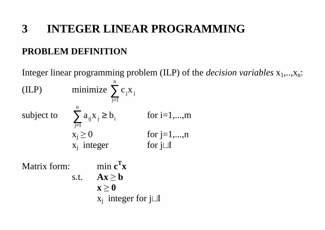
3 INTEGER LINEAR PROGRAMMING

PROBLEM DEFINITION

Integer linear programming problem (ILP) of the decision variables x1,..,xn:

(ILP) minimize ∑=

n

1jjjxc

subject to ∑=

≥n

1jijij bxa for i=1,...,m

xj 0 for j=1,...,nxj integer for j∈I

Matrix form: min cTxs.t. Ax b

x 0xj integer for j∈I

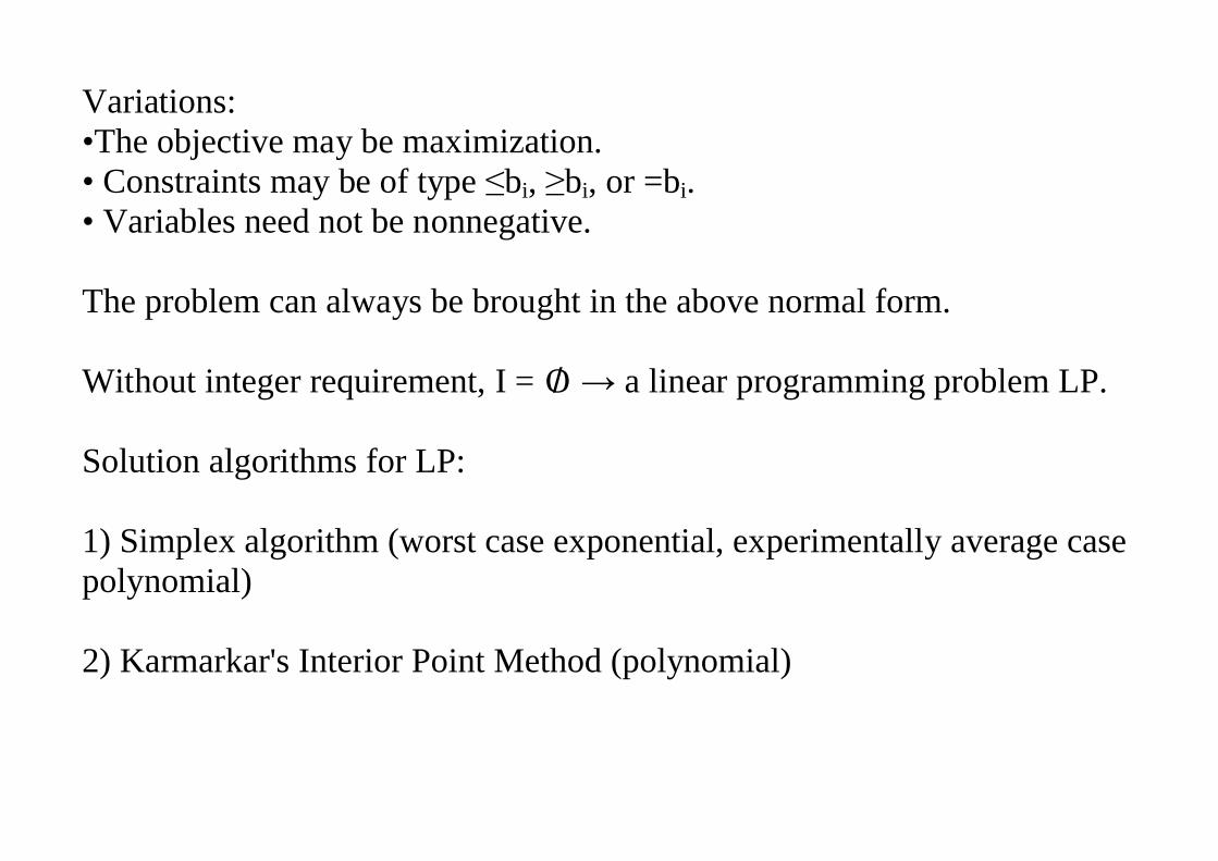
Variations:•The objective may be maximization.• Constraints may be of type bi, bi, or =bi.• Variables need not be nonnegative.

The problem can always be brought in the above normal form.

Without integer requirement, I = O/ a linear programming problem LP.

Solution algorithms for LP:

1) Simplex algorithm (worst case exponential, experimentally average casepolynomial)

2) Karmarkar's Interior Point Method (polynomial)

Subcategories:• Pure integer programming problem: I = {1,...,n}• Mixed integer (linear) programming problem MIP (MILP): some of thevariables are continuous, some integer.• Binary integer programming problem (BIP): xi ∈ {0,1}, i=1,...,n.

All of these are NP-complete:

ILP, MIP, BIP, ... ∈ NPC.

LP-relaxation = ILP without integer requirements

Why linear models?

• The LP-relaxation of linear IP-models can be solved efficiently and thissolution can be used as a starting point for integer solutions.

• Many (most) combinatorial optimization problems can be modeled asILP-models.

• Problems with nonlinear objective or constraint functions are uncommonin combinatorial optimization.

Applications of ILP-models:

- standard graph, routing, packing and scheduling problems of discrete optimization Examples (1)-(14) in Chapter 1.3.

- LP problems in which the variables are numbers of whole pieces.

- LP problems with logical constraints (disjunction, implication etc.), fixed costs

A simple heuristic:Solve the LP-relaxation and round the variables xj, j∈ I to the nearestinteger. Improvement: Try all rounding possibilities.

This technique is suitable only for instances with few integer variables orwhen their order of magnitude is large enough.

Problems:- The rounded solution is not necessarily optimal or may be far from theoptimum.- The rounded solution may not be feasible.- If the number of integer variables is k, the number of different roundingcombinations is 2k. Exponential time, if feasibility has to be checked for all.- Binary variables: no realistic interpretation for fractional values.For example Knapsack problem:xi = 0.5: gives no information of the decision: to take the object or not?The rounding corresponds to a flip of a coin.

BRANCH AND BOUND METHODS

The advantage of a unique model: a general purpose Branch and Boundmethod.

Two basic stages of a general Branch and Bound method:•Branching: splitting the problem into subproblems•Bounding: calculating lower and/or upper bounds for the objectivefunction value of the subproblem

Example of branching: separating the current subspace into two parts usingthe integrality requirement. Using the bounds, unpromising subproblemscan be eliminated.

LP-relaxation:- discarding the integer requirements.- for binary variables, add bounds 0 xi 1

The LP-minimum gives a lower bound for the ILP-minimum:min fLP min fILP.

Incumbent solution = the best IP-solution given by the solved subproblems(record holder).

The incumbent objective value is an upper bound for the minimum value.

A list P of candidate subproblems is maintained and updated.

Subproblem is fathomed (totally solved, examined, explored) and removedfrom the list, when• it has an integer solution that is best so far and becomes the newincumbent solution, or,• its optimum LP-solution objective is worse than the current incumbentvalue, or,• the LP-problem is infeasible.

Notation:f* = minimum value of the objective function for the current

LP-subproblemfmin = incumbent minimum value, given by a feasible integer solution xminP = the set of non-fathomed subproblems

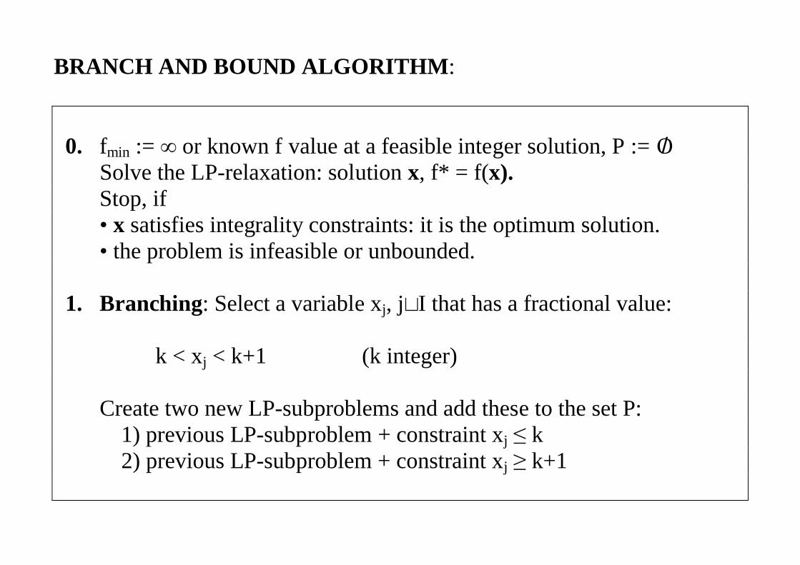
BRANCH AND BOUND ALGORITHM:

0. fmin := or known f value at a feasible integer solution, P := O/ Solve the LP-relaxation: solution x, f* = f(x). Stop, if •x satisfies integrality constraints: it is the optimum solution. • the problem is infeasible or unbounded.

1. Branching: Select a variable xj, j∈I that has a fractional value:

k < xj < k+1 (k integer)

Create two new LP-subproblems and add these to the set P: 1) previous LP-subproblem + constraint xj k

2) previous LP-subproblem + constraint xj k+1

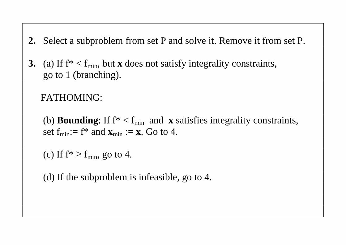
2. Select a subproblem from set P and solve it. Remove it from set P.

3. (a) If f* < fmin, but x does not satisfy integrality constraints, go to 1 (branching).

FATHOMING:

(b) Bounding: If f* < fmin and x satisfies integrality constraints, set fmin:= f* and xmin := x. Go to 4.

(c) If f* fmin, go to 4.

(d) If the subproblem is infeasible, go to 4.

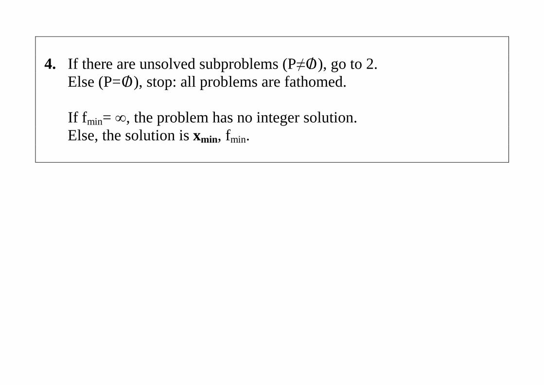
4. If there are unsolved subproblems (P O/ ), go to 2. Else (P=O/ ), stop: all problems are fathomed.

If fmin= , the problem has no integer solution. Else, the solution is xmin, fmin.

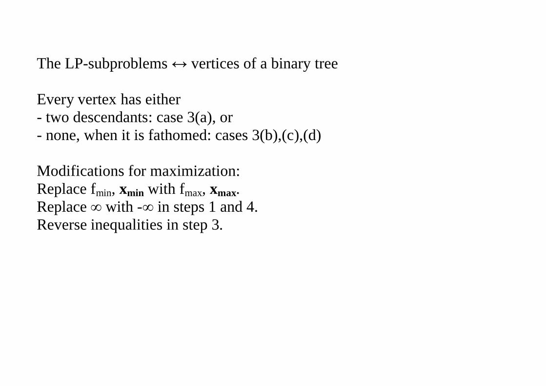
The LP-subproblems vertices of a binary tree

Every vertex has either- two descendants: case 3(a), or- none, when it is fathomed: cases 3(b),(c),(d)

Modifications for maximization:Replace fmin, xmin with fmax, xmax.Replace with - in steps 1 and 4.Reverse inequalities in step 3.

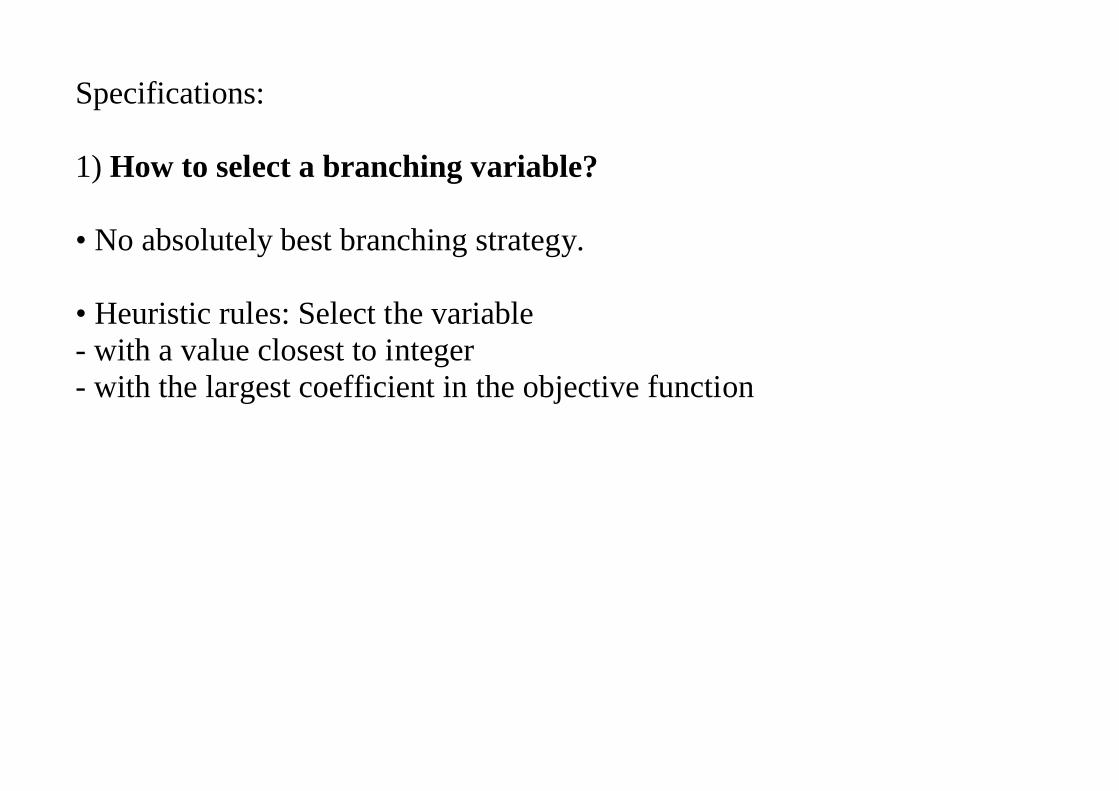
Specifications:

1) How to select a branching variable?

• No absolutely best branching strategy.

• Heuristic rules: Select the variable- with a value closest to integer- with the largest coefficient in the objective function

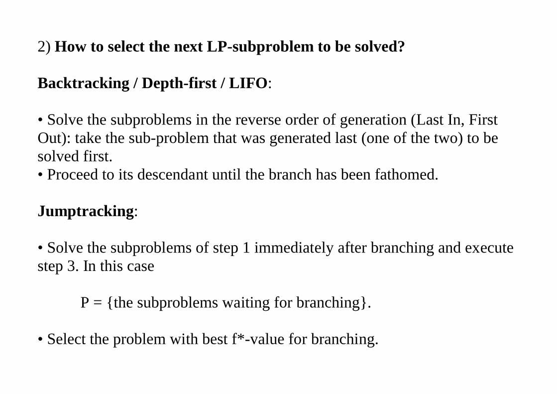
2) How to select the next LP-subproblem to be solved?

Backtracking / Depth-first / LIFO:

• Solve the subproblems in the reverse order of generation (Last In, FirstOut): take the sub-problem that was generated last (one of the two) to besolved first.• Proceed to its descendant until the branch has been fathomed.

Jumptracking:

• Solve the subproblems of step 1 immediately after branching and executestep 3. In this case

P = {the subproblems waiting for branching}.

• Select the problem with best f*-value for branching.

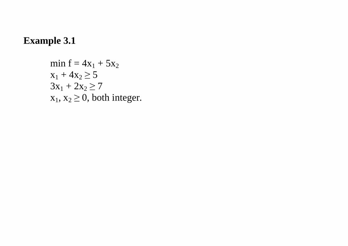
Example 3.1

min f = 4x1 + 5x2x1 + 4x2 53x1 + 2x2 7x1, x2 0, both integer.

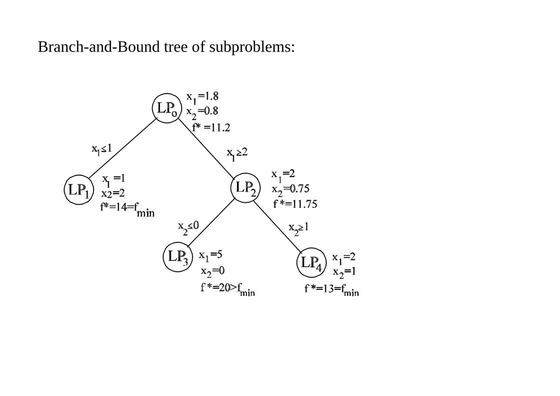
Branch-and-Bound tree of subproblems:

Comment:The descendant LP-subproblem differ from its parent LP-problem only byone constraint

Use dual simplex method, starting from the basic solution of its parent LP.

The above Branch & Bound can be used for pure ILP:s, mixed ILP:s andbinary problems.

For binary variables the branching constraints xi 0 and xi 1 result invalues xi=0 and xi=1.

Implicit enumeration techniques like Balas' additive algorithm may becomputationally more efficient for binary problems.

Specialized implementations of the B&B method exist for commonproblem types of Chapter 1.3 e.g. TSP or scheduling.

General goals of all Branch & Bound methods:

• to determine the bounds as tight as possible• efficient fathoming of subproblems = pruning of nonpromising branches• to keep the total computation time at minimum

The last goal in conflict with the first two:tight bounds mean efficient fathoming but more computation per vertex.

CUTTING PLANE METHODS

Consider a pure integer linear programming problem, where all parametersare integers.

This can be accomplished by multiplying a constraint by a suitableconstant.

Objective function value and all the "slack" variables have integer values(in a feasible solution).

First, solve the LP-relaxation to get a lower bound for the minimumobjective value.

Final simplex tableau given: basic variables have columns with coefficient1 in one constraint row and 0 in other rows.

Solution:• nonbasic variables = 0• basic varibles = RHS (right hand side)

The objective function of the same form, basic variable f.

If the LP-solution is fractional, at least one of the RHS values is fractional.

Append to the model a constraint that cuts away a part of the feasible set,so that no integer solutions are lost.

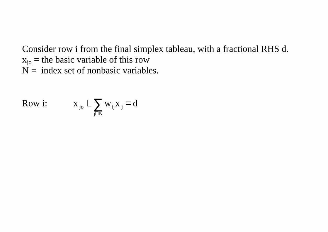
Consider row i from the final simplex tableau, with a fractional RHS d.xjo = the basic variable of this rowN = index set of nonbasic variables.

Row i: dxwxNj

jijjo =+ ∑∈

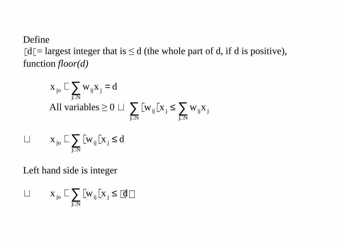
Define d = largest integer that is d (the whole part of d, if d is positive),function floor(d)

dxwxNj

jijjo =+ ∑∈

All variables 0 ⇒ ∑ ∑∈ ∈

≤Nj Nj

jijjij xwxw

⇒ ∑∈

≤+Nj

jijjo dxwx

Left hand side is integer

⇒ ∑∈

≤+Nj

jijjo dxwx

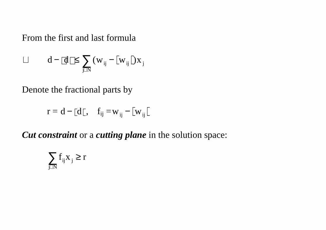
From the first and last formula

⇒ ∑∈

−≤−Nj

jijij x)ww(dd

Denote the fractional parts by

r = dd − , fij = ijij ww −

Cut constraint or a cutting plane in the solution space:

∑∈

≥Nj

jij rxf

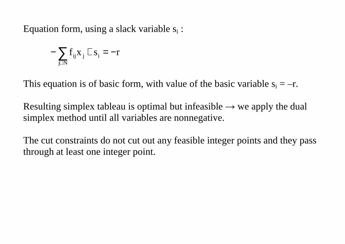
Equation form, using a slack variable si :

∑∈

−=+−Nj

ijij rsxf

This equation is of basic form, with value of the basic variable si = –r.

Resulting simplex tableau is optimal but infeasible we apply the dualsimplex method until all variables are nonnegative.

The cut constraints do not cut out any feasible integer points and they passthrough at least one integer point.

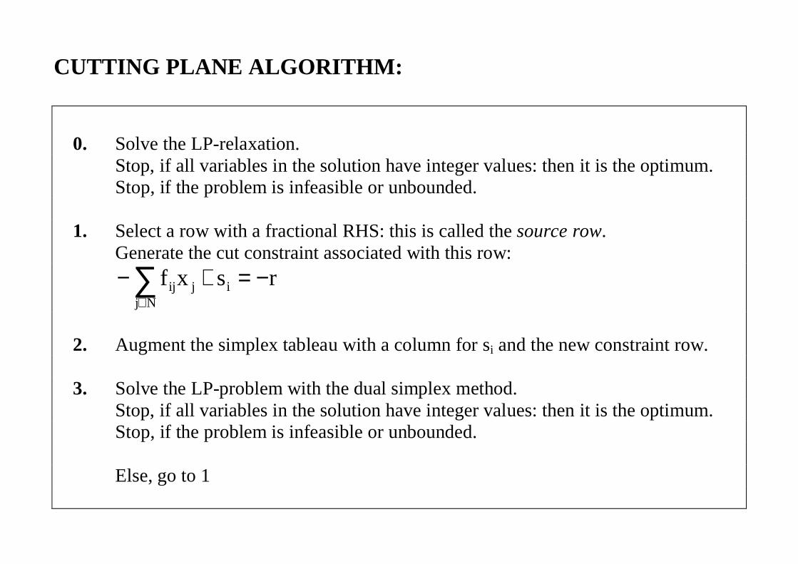
CUTTING PLANE ALGORITHM:

0. Solve the LP-relaxation.Stop, if all variables in the solution have integer values: then it is the optimum.Stop, if the problem is infeasible or unbounded.

1. Select a row with a fractional RHS: this is called the source row.Generate the cut constraint associated with this row:

∑∈

−=+−Nj

ijij rsxf

2. Augment the simplex tableau with a column for si and the new constraint row.

3. Solve the LP-problem with the dual simplex method.Stop, if all variables in the solution have integer values: then it is the optimum.Stop, if the problem is infeasible or unbounded.

Else, go to 1

The source row can be chosen arbitrarily. Also the objective row can beused because the value of f must be integer.

If a cut constraint becomes inactive again with si > 0, then variable si and itsrow can be eliminated from the tableau. This means a new cut makes theold one unnecessary. The elimination restricts the growth of the simplextableau.

The number of iterations is difficult to estimate but being an exact methodlike the B&B, the computation time is not polynomially bounded.

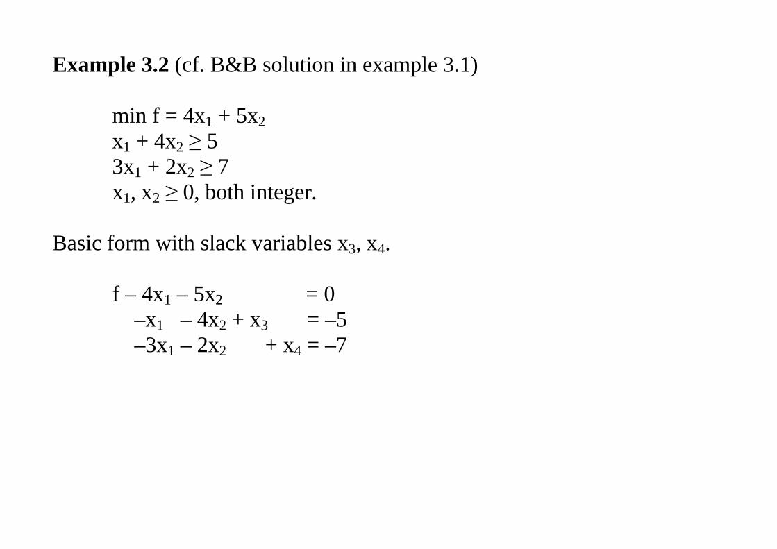
Example 3.2 (cf. B&B solution in example 3.1)

min f = 4x1 + 5x2x1 + 4x2 53x1 + 2x2 7x1, x2 0, both integer.

Basic form with slack variables x3, x4.

f – 4x1 – 5x2 = 0 –x1 – 4x2 + x3 = –5 –3x1 – 2x2 + x4 = –7

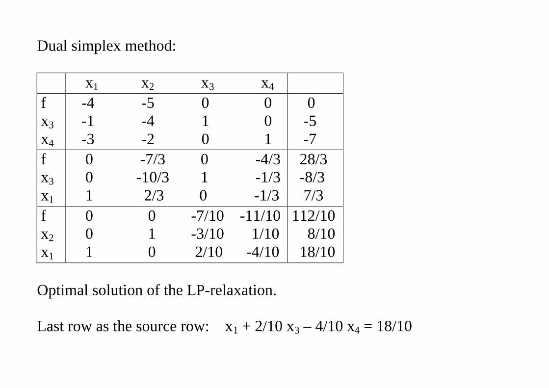
Dual simplex method:

x1 x2 x3 x4

fx3x4

-4 -5 0 0 -1 -4 1 0 -3 -2 0 1

0 -5 -7

fx3x1

0 -7/3 0 -4/3 0 -10/3 1 -1/3 1 2/3 0 -1/3

28/3 -8/3 7/3

fx2x1

0 0 -7/10 -11/10 0 1 -3/10 1/10 1 0 2/10 -4/10

112/10 8/10 18/10

Optimal solution of the LP-relaxation.

Last row as the source row: x1 + 2/10 x3 – 4/10 x4 = 18/10

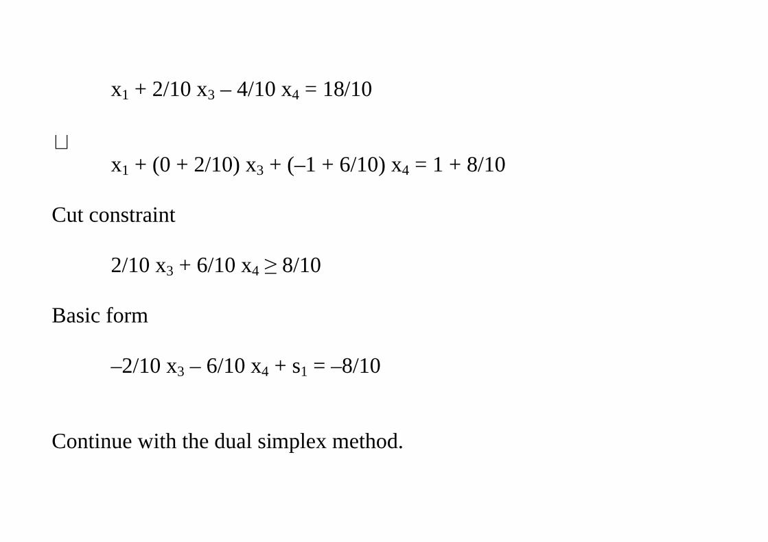
x1 + 2/10 x3 – 4/10 x4 = 18/10

⇔x1 + (0 + 2/10) x3 + (–1 + 6/10) x4 = 1 + 8/10

Cut constraint

2/10 x3 + 6/10 x4 8/10

Basic form

–2/10 x3 – 6/10 x4 + s1 = –8/10

Continue with the dual simplex method.

x1 x2 x3 x4 s1

fx2x1s1

0 0 -7/10 -11/10 0 0 1 -3/10 1/10 0 1 0 2/10 -4/10 0 0 0 -2/10 -6/10 1

112/10 8/10 18/10 -8/10

fx2x1x4

0 0 -2/6 0 -11/6 0 1 -2/6 0 1/6 1 0 2/6 0 -4/6 0 0 2/6 1 -10/6

76/6 4/6 14/6 8/6

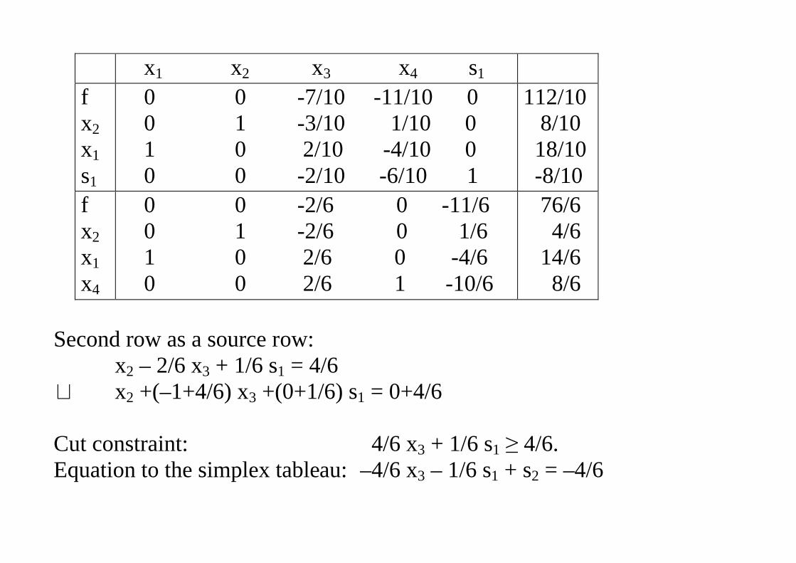
Second row as a source row:x2 – 2/6 x3 + 1/6 s1 = 4/6

⇔ x2 +(–1+4/6) x3 +(0+1/6) s1 = 0+4/6

Cut constraint: 4/6 x3 + 1/6 s1 4/6.Equation to the simplex tableau: –4/6 x3 – 1/6 s1 + s2 = –4/6

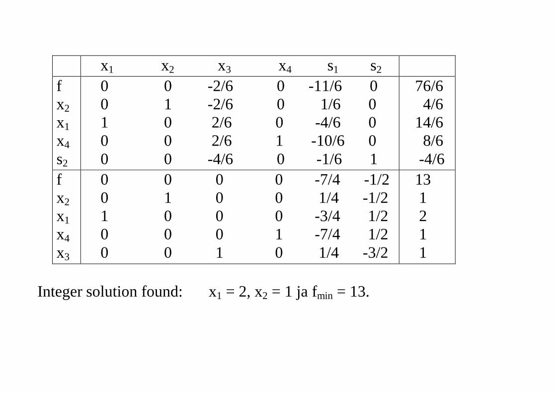
x1 x2 x3 x4 s1 s2

fx2x1x4s2

0 0 -2/6 0 -11/6 0 0 1 -2/6 0 1/6 0 1 0 2/6 0 -4/6 0 0 0 2/6 1 -10/6 0 0 0 -4/6 0 -1/6 1

76/6 4/6 14/6 8/6 -4/6

fx2x1x4x3

0 0 0 0 -7/4 -1/2 0 1 0 0 1/4 -1/2 1 0 0 0 -3/4 1/2 0 0 0 1 -7/4 1/2 0 0 1 0 1/4 -3/2

13 1 2 1 1

Integer solution found: x1 = 2, x2 = 1 ja fmin = 13.

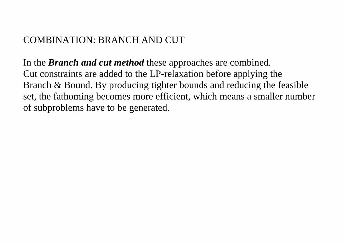
COMBINATION: BRANCH AND CUT

In the Branch and cut method these approaches are combined.Cut constraints are added to the LP-relaxation before applying theBranch & Bound. By producing tighter bounds and reducing the feasibleset, the fathoming becomes more efficient, which means a smaller numberof subproblems have to be generated.