3. THE EXCHANGE ECONOMY - Essential …essentialmicroeconomics.com/ChapterY3/SlideChapter3.pdf · 3. THE EXCHANGE ECONOMY ... If preferences are CES with elasticity of substitution

Essential Microeconomics -1-

© John Riley

3. THE EXCHANGE ECONOMY

Pareto efficient allocations 2

Edgeworth box analysis 5

Market clearing prices 13

Walrasian Equilibrium 16

Equilibrium and Efficiency 22

First welfare theorem 24

Second welfare theorem (convex, differentiable economy) 28

The homothetic preference 2 2× economy 41

Second welfare theorem (convex economy) 49


© John Riley

Private goods exchange economy

Consumer (or household) , 1,...,h h H= has strictly increasing preferences h

over h nX += .

We assume that the basic preference axioms are satisfied so that these are represented by a continuous

utility function ( )hU ⋅ .

Where it is helpful we will assume that U is continuously differentiable ( 1( )U ⋅ ∈ ).

Endowments: The initial allocation of commodities is 1{ }h Hhω = .

Feasible allocations: The final allocation 1{ }h Hhx = is feasible if

1 1

H Hh h

h hx ω

= =

≤∑ ∑

*


© John Riley

Private goods exchange economy

Consumer (or household) , 1,...,h h H= has strictly increasing preferences h

over h nX += .

We assume that the basic preference axioms are satisfied so that these are represented by a continuous

utility function ( )hU ⋅ .

Where it is helpful we will assume that U is continuously differentiable ( 1( )U ⋅ ∈ ).

Endowments: The initial allocation of commodities is 1{ }h Hhω = .

Feasible allocations: The final allocation 1{ }h Hhx = is feasible if

1 1

H Hh h

h hx ω

= =

≤∑ ∑

Pareto-efficient allocations

An allocation 1ˆ{ }h Hhx = is Pareto efficient if there is no other feasible allocation in which at least one

consumer is strictly better off and no consumer is worse off.

Consider an alternative allocation 1{ }h Hhx = in which consumers 2,…,H are all at least as well off.

That is, ˆˆ( ) ( )h h h h hU x U x U≥ ≡

Then 1 1 1 1ˆ( ) ( )U x U x≥ and so 1ˆ{ }h Hhx = solves the following maximization problem.

1 1 1

{ } 1 1

ˆˆ arg { ( ) | ( ) , 2,..., , }h

H Hh h h h h

x h hx Max U x U x U h H x ω

= =

= ≥ = ≤∑ ∑


© John Riley

Two commodity 2 consumer case (Alex and Bev)

For the special 2 2× case, Alex and Bev must

share the aggregate endowment 1 2( , )ω ω ω= .

Let ˆBx be the allocation to Bev and let B̂ be the set

of allocations that Bev prefers over ˆBx .

This is depicted in Figure 3.1-2. For any ˆBx B∈ ,

the allocation to Alex is A Bx xω= − . Thus the best

possible allocation to Alex that leaves Bev no worse

off is Alex’s utility maximizing allocation in B̂ .

Figure 3.1-2: Bev’s upper contour set


© John Riley

Edgeworth box diagram

Since preferences are strictly increasing

a PE allocation uses all the endowment A B A Bx x ω ω ω+ = = +

In the diagram the sum of the two consumption

vectors is the vector 1 2( , )ω ω , that is, the right

hand corner of the Edgeworth box.

Figure 3.1-3: Edgeworth box Diagram


© John Riley

For Pareto-efficiency, there can be no mutually

preferred alternative. One PE allocation is

depicted in Figure 3.1-4. As long as an allocation

ˆ ˆ ˆ{ , }A B Ax x xω= −

is in the interior of the Edgeworth box, a necessary

condition for the allocation to be PE is that the

slopes of the two indifference curves must be

equal. Thus the graph of the PE allocations is the set

of allocations to Alex (and hence Bev) satisfying

1 1

2 2

ˆ ˆ( ) ( )ˆ( )

ˆ ˆ( ) ( )

A BA B

A AA B

A B

U Ux xx xMRS x

U Ux xx x

∂ ∂∂ ∂

= =∂ ∂∂ ∂

, where ˆ Â Bx x ω+ = .

Figure 3.1-4: PE allocations with identical CES preferences


© John Riley

Example: Identical CES Preferences

If preferences are CES with elasticity of

substitution σ , Alex and Bev have a 1/

2

1

( )h

h hh

xMRS x kx

σ⎛ ⎞

= ⎜ ⎟⎝ ⎠

.

For a PE allocation in the interior of the Edgeworth

box, the indifference curves of the two consumers

must have the same slope, that is, 1/ 1/

2 2

1 1

A B

A B

x xx x

σ σ⎛ ⎞ ⎛ ⎞

=⎜ ⎟ ⎜ ⎟⎝ ⎠ ⎝ ⎠

hence 2 2

1 1

A B

A B

x xx x

= .

*



© John Riley

Example: Identical CES Preferences

If preferences are CES with elasticity of

substitution σ , Alex and Bev have a 1/

2

1

( )h

h hh

xMRS x kx

σ⎛ ⎞

= ⎜ ⎟⎝ ⎠

.

For a PE allocation in the interior of the Edgeworth

box, the indifference curves of the two consumers

must have the same slope, that is, 1/ 1/

2 2

1 1

A B

A B

x xx x

σ σ⎛ ⎞ ⎛ ⎞

=⎜ ⎟ ⎜ ⎟⎝ ⎠ ⎝ ⎠

hence 2 2

1 1

A B

A B

x xx x

= .

Ratio Rule: 1 1 1 1

2 2 2 2

a b a ba b a b

+= =

+

Proof: If 1 1

2 2

a b ka b

= = then 1 2a ka= and 1 2b kb= and so 1 1 2 2( )a b k a b+ = + .

Hence 1 1

2 2

a b ka b+

=+

.



© John Riley

Appealing to the Ratio Rule and then setting

demand equal to supply,

2 2 2 2 2

1 1 1 1

A B A B

A B A Ba

x x x xx x x x

ωω

+= = =

+.

Thus, in a PE allocation each consumer is

allocated a fraction of the aggregate endowment.

It follows that for each consumer the marginal

rate of substitution is 1/

2

1

ˆ( )h hMRS x kσ

ωω

⎛ ⎞= ⎜ ⎟

⎝ ⎠. (3.1-1)

The PE allocations are depicted in Figure 3.1-4.



© John Riley

Walrasian Equilibrium for an Exchange Economy

Let 0p ≥ be a price vector of this exchange economy.

In a WE each consumer is a price taker.

We write the set of consumers as {1,..., }HH= .

***


© John Riley





We assume that preferences are strictly convex so consumer h has is a unique most preferred

consumption vector, ( , )h hx p ω .

( , ) arg { ( ) | }h h h h

xx p Max U x p x pω ω= ⋅ ≤ ⋅ .

**


© John Riley







( , ) arg { ( ) | }h h h h


Total endowment vector: h

hω ω

∈

= ∑H

Total or “market” demand: ( ) ( , )h h

hx p x p ω

∈

= ∑H

Excess demand: ( ) ( )z p x p ω= − .

*


© John Riley







( , ) arg { ( ) | }h h h h


Total endowment vector: h

hω ω

∈

= ∑H

Total or “market” demand: ( ) ( , )h h

hx p x p ω

∈

= ∑H

Excess demand: ( ) ( )z p x p ω= − .

Definition: Market Clearing Prices

Let ( )jz p be the excess demand for commodity j at the price vector 0p ≥ . The market for commodity

j clears if ( ) 0jz p ≤ and ( ) 0j jp z p = .


© John Riley

Walras’ Law: If preferences satisfy local non-satiation and all markets but one clear then the

remaining market must also clear.

If preferences satisfy local non-satiation, then a consumer must spend all of his income.

Why is this?

**


© John Riley




Why is this?

Then for any price vector p the market value of excess demands must be zero.

( ) ( ) ( ( )) ( )h h h h

h hp z p p x p x p x pω ω ω

∈ ∈

⋅ = ⋅ − = ⋅ − = ⋅ − ⋅∑ ∑H H

.

Because all consumers spend their entire wealth the right hand expression is zero. Hence

1

( ) ( ) ( ) 0n

i i j jjj i

p z p p z p p z p=≠

⋅ = + =∑ .

*


© John Riley




Why is this?

Then for any price vector p the market value of excess demands must be zero.

( ) ( ) ( ( )) ( )h h h h

h hp z p p x p x p x pω ω ω

∈ ∈

⋅ = ⋅ − = ⋅ − = ⋅ − ⋅∑ ∑H H

.

Because all consumers spend their entire wealth the right hand expression is zero. Hence

1

( ) ( ) ( ) 0n

i i j jjj i

p z p p z p p z p=≠

⋅ = + =∑ .

Therefore if all markets but market i clear then market i must clear as well.

Definition: Walrasian Equilibrium price vector

The price vector 0p ≥ is a WE price vector if all markets clear.


© John Riley

Edgeworth box example

In a Walrasian equilibrium consumers choose

the best point in their budget sest given a price

vector 1 2( , )p p p= .

In the figure these are the lightly shaded orange

and green triangles.

**

Figure 3.1-5: Excess supply of commodity 1

N


© John Riley



the best point in their budget set given a price

vector 1 2( , )p p p= .



It is very important to note that consumers consider

only their budget sets. In the case depicted, both of

these budget sets extend beyond the boundary of the

Edgeworth box (the set of feasible allocations).

*


N


© John Riley



the best point in their budget set given a price

vector 1 2( , )p p p= .



It is very important to note that consumers consider

only their budget sets. In the case depicted, both of

these budget sets extend beyond the boundary of the

Edgeworth box (the set of feasible allocations).

The heavily shaded triangles indicate the desired trades

of the two consumers. As depicted, Alex

wants to trade from the endowment point N to his most preferred desired consumption Ax , whereas

Bev wishes to trade from N to Bx . Thus, there is excess supply of commodity 1.


N


© John Riley

By lowering the price of commodity 1 (relative to

commodity 2) the budget line becomes less steep

until eventually supply equals demand. The

Walrasian equilibrium E is depicted in Figure 3.1-6.

Figure 3.1-6: Walrasian equilibrium

N


© John Riley

Class Exercise: Which (if any) of these figures depicts a Walrasian equilibrium?

In the left figure the budget line is tangential to Bev’s indifference curve at ˆ Ax .

In the right-hand figure the budget line is tangential to Alex’s indifference curve.


© John Riley

Equilibrium and Efficiency

In Figure 3.1-6 the WE allocation is in the interior of the

Edgeworth box. Thus the marginal rates of substitution

must both be equal to the price ratio:

1 1 1

2

2 2

( ) ( )( ) ( )

( ) ( )

A BA B

A A B BA B

A B

U Ux xx p xMRS x MRS x

U Upx xx x

∂ ∂∂ ∂

= = = =∂ ∂∂ ∂

Since the MRS are equal, it follows that the

WE allocation must be PE.

*


N


© John Riley

Equilibrium and Efficiency

In Figure 3.1-6 the WE allocation is in the interior of the

Edgeworth box. Thus the marginal rates of substitution

must both be equal to the price ratio:

1 1 1

2

2 2

( ) ( )( ) ( )

( ) ( )

A BA B

A A B BA B

A B

U Ux xx p xMRS x MRS x

U Upx xx x

∂ ∂∂ ∂

= = = =∂ ∂∂ ∂

Since the MRS are equal, it follows that the

WE allocation must be PE.

To prove that this result holds very generally, we will appeal to the Duality Lemma (Section 2.2). That

is, if the local non-satiation property holds, then the utility-maximizing bundle is cost minimizing

among all preferred consumption bundles.

Duality Lemma

arg { ( ) | }h

h h h h h

xx Max U x p x p ω= ⋅ ≤ ⋅ ⇒ { | ( ) ( )}

h

h h h h h h

xp x Min p x U x U x⋅ = ⋅ ≥ .


N


© John Riley

Proposition 3.1-2: First welfare theorem for an exchange economy

If preferences satisfy local non-satiation, a WE allocation in an exchange economy is PE.

Proof: Let { }hhx ∈H be a WE allocation for the exchange economy with endowments { }h

hω ∈H . Let

0p ≥ be the WE price vector.

Consider any allocation { }hhx ∈H that is Pareto-preferred to { }h

hx ∈H . Because none of the consumers

can be worse off in the Pareto-preferred allocation, it follows from the Duality Lemma that

0, .h hp x p x h⋅ − ⋅ ≥ ∈H

**


© John Riley




hω ∈H . Let





0, .h hp x p x h⋅ − ⋅ ≥ ∈H

Moreover at least one consumer must be strictly better off. Since hx is the most preferred allocation in

the budget set, it follows that

0h hp x p x⋅ − ⋅ > , for some h .

*


© John Riley




hω ∈H . Let





0, .h hp x p x h⋅ − ⋅ ≥ ∈H

Moreover at least one consumer must be strictly better off. Since hx is the most preferred allocation in

the budget set, it follows that

0h hp x p x⋅ − ⋅ > , for some h .

Summing over consumers,

( ) 0h h

h hp x x

∈ ∈

⋅ − >∑ ∑H H

.

Also all markets clear in a Walrasian equilibrium. Therefore

( ) 0h h

h hp x p ω

∈ ∈

⋅ − ⋅ =∑ ∑H H

.


© John Riley

Combining these results,

0h h

h hp x ω

∈ ∈

⎛ ⎞⋅ − >⎜ ⎟⎝ ⎠∑ ∑H H

Because 0p ≥ , it follows that there must be some commodity j such that 0h hj j

h hx ω

∈ ∈

− >∑ ∑H H

. Thus

all Pareto-preferred allocations are infeasible.

Q.E.D.


© John Riley

Second Welfare Theorem

We now argue that, as long as preferences are convex,

any PE allocation is also a WE allocation for some

redistribution of resources.

Consider the PE allocation ˆ ˆ,A Bx x where ˆ Â Bx x ω+ = in Figure 3.1-7. The shaded regions are the allocations

where either Alex or Bev is better off.

**

Figure 3.1-7: PE allocation


© John Riley







If preferences are convex, each of these sets is convex so,

by the Separating Hyperplane Theorem, we can draw a line

Â Ap x p x⋅ = ⋅ through ˆ Ax separating the two sets.

*



© John Riley







If preferences are convex, each of these sets is convex so,

by the Separating Hyperplane Theorem, we can draw a line

Â Ap x p x⋅ = ⋅ through ˆ Ax separating the two sets.

If the endowments are ˆ ˆ ,h hx hω = ∈H each individual maximizes by choosing his or her endowment.

Because demand equals supply for each individual, all markets clear. Thus the price vector p is a WE

price vector.



© John Riley

Define the transfer payment ˆ( ),h h hT p x hω= ⋅ − ∈H .

Because ˆh h

h h

x ω∈ ∈

=∑ ∑H H

the sum of these transfers is zero so this is a feasible redistribution of wealth.

The budget constraint ˆh hp x p x⋅ ≤ ⋅ can be rewritten as follows: h h hp x p Tω⋅ ≤ ⋅ + .

Then given transfers ,hT h∈H , the price vector p is a WE price vector.


© John Riley

Proposition 3.1-3: Second welfare theorem for an exchange economy

In an exchange economy with endowments ,{ }hhω ∈H , suppose that ( )hU x , is continuously

differentiable, quasi concave on n+and that ( ) 0

hh

h

U xx

∂>>

∂ , h∈H . Then any PE allocation ˆ{ }h

hx ∈H

where ˆ 0,hx h≠ ∈H , can be supported by a price vector 0p > .

For expositional simplicity, consider a two person economy. The generalization is direct.

The idea on the proof is to argue that a PE allocation must be the solution to a maximization problem

and then show that the associated shadow prices are no-trade WE prices.

*


© John Riley

Proposition 3.1-3: Second welfare theorem for an exchange economy

In an exchange economy with endowments ,{ }hhω ∈H , suppose that ( )hU x , is continuously

differentiable, quasi concave on n+and that ( ) 0

hh

h

U xx

∂>>

∂ , h∈H . Then any PE allocation ˆ{ }h

hx ∈H

where ˆ 0,hx h≠ ∈H , can be supported by a price vector 0p > .

For expositional simplicity, consider a two person economy. The generalization is direct.

The idea on the proof is to argue that a PE allocation must be the solution to a maximization problem

and then show that the associated shadow prices are no-trade WE prices.

Proof: If ˆ ˆ,A Bx x is a PE allocation then

,

ˆ ârg { ( ) | , ( ) ( )}A B

A A A A B A B B B B B

x xx Max U x x x U x U xω ω= + ≤ + ≥ . (3.1-2)

Class exercise: Explain why the assumptions imply that the Kuhn-Tucker conditions are necessary

conditions.


© John Riley

The Lagrangian for the optimization problem (3.1-2) is

ˆ( ) ( ) ( ( ) ( ))A A A B A B B B B BU x x x U x U xν ω ω μ= + + − − + −L .

Kuhn-Tucker conditions.

ˆ( ) 0A

AA A

U xx x

ν∂ ∂= − ≤

∂ ∂L , where ˆ ˆ( ( ) ) 0

AA A

A

Ux xx

ν∂⋅ − =∂

. (3.1-3)

ˆ( ) 0B

BB A

U xx x

μ ν∂ ∂= − ≤

∂ ∂L , where ˆ ˆ( ( ) ) 0

BB B

B

Ux xx

μ ν∂⋅ − =

∂. (3.1-4)

ˆ ˆ 0A B A Bx xω ων∂

= + − − ≥∂L , where ˆ ˆ( ) 0A B A Bx xν ω ω⋅ + − − = . (3.1-5)

***


© John Riley




ˆ( ) 0A

AA A

U xx x

ν∂ ∂= − ≤

∂ ∂L , where ˆ ˆ( ( ) ) 0

AA A

A

Ux xx

ν∂⋅ − =∂

. (3.1-3)

ˆ( ) 0B

BB A

U xx x

μ ν∂ ∂= − ≤

∂ ∂L , where ˆ ˆ( ( ) ) 0

BB B

B

Ux xx

μ ν∂⋅ − =

∂. (3.1-4)



Because 0A

A

Ux

∂>>

∂ it follows from (3.1-3) that 0ν >> . From (3.1-5) it then follows that

ˆ ˆ 0A B A Bx xω ω+ − − = . (3.1-6)

**


© John Riley




ˆ( ) 0A

AA A

U xx x

ν∂ ∂= − ≤

∂ ∂L , where ˆ ˆ( ( ) ) 0

AA A

A

Ux xx

ν∂⋅ − =∂

. (3.1-3)

ˆ( ) 0B

BB A

U xx x

μ ν∂ ∂= − ≤

∂ ∂L , where ˆ ˆ( ( ) ) 0

BB B

B

Ux xx

μ ν∂⋅ − =

∂. (3.1-4)



Because 0A

A

Ux

∂>>


ˆ ˆ 0A B A Bx xω ω+ − − = . (3.1-6)

Because ˆ 0Bx > and 0B

B

Ux

∂>>

∂ it follows from (3.1-4) that 0μ > .

*


© John Riley




ˆ( ) 0A

AA A

U xx x

ν∂ ∂= − ≤

∂ ∂L , where ˆ ˆ( ( ) ) 0

AA A

A

Ux xx

ν∂⋅ − =∂

. (3.1-3)

ˆ( ) 0B

BB A

U xx x

μ ν∂ ∂= − ≤

∂ ∂L , where ˆ ˆ( ( ) ) 0

BB B

B

Ux xx

μ ν∂⋅ − =

∂. (3.1-4)



Because 0A

A

Ux

∂>>


ˆ ˆ 0A B A Bx xω ω+ − − = . (3.1-6)

Because ˆ 0Bx > and 0B

B

Ux

∂>>

∂ it follows from (3.1-4) that 0μ > .

Now consider an economy with endowments ˆ ˆh hxω = , h∈H and consider the price vector p ν= .


© John Riley

Consumer h chooses ârg { ( ) | }h

h h h h h

xx Max U x x xν ν= ⋅ ≤ ⋅ .

The FOC for this optimization problem are

( ) 0h

h hh h

U xx x

λ ν∂ ∂= − ≤

∂ ∂L , where ( ( ) ) 0

hh h h

h

Ux xx

λ ν∂− =

∂.

Moreover, because ( )hU ⋅ is quasi-concave the FOC is also sufficient. Choose 1Aλ = and 1/Bλ μ= .

Then, appealing to (3.1-3) and (3.1-4), the FOC hold at ˆ ,h hx x h= ∈H .

**


© John Riley


h h h h h



( ) 0h

h hh h

U xx x

λ ν∂ ∂= − ≤

∂ ∂L , where ( ( ) ) 0

hh h h

h

Ux xx

λ ν∂− =

∂.



Thus at the price p ν= no consumer wishes to trade. Therefore supply equals demand and so the price

vector is a WE price vector.

*


© John Riley


h h h h h



( ) 0h

h hh h

U xx x

λ ν∂ ∂= − ≤

∂ ∂L , where ( ( ) ) 0

hh h h

h

Ux xx

λ ν∂− =

∂.



Thus at the price p ν= no consumer wishes to trade. Therefore supply equals demand and so the price

vector is a WE price vector.

Finally define transfers ˆ( )h h hT xν ω= ⋅ − . Appealing to (3.1-2), the sum of these transfers is zero.

Consumer h’s budget constraint with these transfers is

ˆh h h hx T xν ν ω ν⋅ ≤ ⋅ + = ⋅ .

Thus the PE allocation is achievable as a WE with the appropriate transfer payments among

consumers.

Q.E.D.


© John Riley

Homothetic Preferences

Suppose that the two individuals in the economy (Alex and Bev) have different convex and

homothetic preferences. At the aggregate endowment, 1 2( , ),ω ω Alex has a stronger preference for

commodity 1 than Bev. That is, Alex is willing to give up more units of commodity 2 than Bev in

exchange for an additional unit of commodity 1.

Assumption: Differing Intensity of preferences

At the aggregate endowment, Alex has a stronger preference for commodity 1 than Bev.

1 2 1 21 2 1 2

( , ) ( , )/ /A A B B

A BU U U UMRS MRSx x x x

∂ ∂ ∂ ∂ω ω ω ω∂ ∂ ∂ ∂

= > = (3.1-7)

This is depicted in Figure 3.1-9.

Figure 3.1-9: Alex has a stronger preference for commodity 1


© John Riley

We now explore the implications of this

assumption for the PE allocations.

Consider the PE allocation C in the

interior of the Edgeworth box.

Class exercises

1. Explain why all PE allocation lie below

the diagonal.

2. Explain why the allocations in the yellow and

dark blue regions are not PE.

Thus any other PE allocation C′preferred by Alex must lie above the line AO D . Because Alex’s MRS

is constant along this line, the marginal rate of substitution at C′ will be higher, reflecting the greater

influence of Alex’s stronger preference for commodity 1. Then

2 2

1 1

,h h

h h

x x hx xC C

< ∈′

H , and ( ) ( ),h hMRS C MRS C h′ > ∈H .

F

D

Commodity 1

Commodity 2

Fig 3.1‐10: Pareto efficient allocations


© John Riley

We summarize these results below.

Proposition 3.1-4: Pareto Efficient Allocations With Homothetic Preferences

In the 2 2× exchange economy, suppose each consumer has homothetic preferences. Suppose also that

at the aggregate endowment, consumer A has a stronger preference for commodity 1. Then at any

interior efficient allocation,

2 2

1 1

A B

A B

x xx x

< .

Moreover, along the locus of efficient allocations, as consumer A’s utility rises, the consumption ratio

2 1/h hx x and marginal rate of substitution of 1x for 2x of both consumers rises.

Note that if Alex become relatively more wealthy so that the WE moves from C to C′ , the equilibrium

MRS rises. Thus 1 2/p p , the equilibrium relative price of commodity 1 rises.

Intuitively, since Alex has a stronger preference for commodity 1, the higher endowment, the more the

relative price reflects his preferences.


© John Riley

A closer look at the second welfare theorem

The economy

Commodities are private: Consumer {1,..., }h H∈ =H has preferences over his own consumption

vector 1( ,...,. )h h hnx x x=

Consumption set: Preferences are defined over the convex set h nX ⊂ .

Endowments: Consumer h has an endowment vector h hXω ∈ .

Consumption allocation: { }hhx ∈H where ,h hx X h∈ ∈H .

Aggregate consumption: h

h

x x∈

= ∑H

.

Aggregate endowment is h

h

ω ω∈

= ∑H

.

Excess demand: z x ω= − z


© John Riley

Feasible Allocation:

An allocation { }hhx ∈H satisfying 0z x ω= − ≤ .

***


© John Riley



Pareto-Efficient Allocation

A feasible allocation ˆ{ }hhx ∈H , is Pareto-efficient if there is no other feasible plan that is strictly

preferred by at least one consumer and weakly preferred by all consumers.

**


© John Riley






Price-Taking

Let 0p ≥ be the price vector. Consumers are price takers. Consumer h has an endowment hω .

She chooses a consumption bundle hx in her budget set { | }h h h hx X p x p ω∈ ⋅ ≤ ⋅ .

*


© John Riley






Price-Taking

Let 0p ≥ be the price vector. Consumers are price takers. Consumer h has an endowment hω .

She chooses a consumption bundle hx in her budget set { | }h h h hx X p x p ω∈ ⋅ ≤ ⋅ .

Walrasian Equilibrium

Each consumer chooses the most preferred consumption plan in her budget set. That is,

( ) ( ), for all such thath h h h h h hU x U x x p x p ω≥ ⋅ ≤ ⋅

Let hx x=∑ be the total consumption of the consumers. Excess demand is then z x ω= − .

Definition: Walrasian equilibrium prices

The price vector 0p ≥ is a Walrasian equilibrium price vector if there is no market in excess

demand ( 0)z ≤ and 0jp = for any market in excess supply ( 0)jz < .


© John Riley

Second welfare theorem

The earlier proof appealed to the Kuhn-Tucker conditions. As we have seen, these follow from the

Supporting Hyperplane Theorem.

We now dispense with differentiability assumption and appeal directly to the Supporting Hyperplane

Theorem.

If ˆ{ }hhx ∈H is PE it ˆ{ }h

hx ∈H must solve the following optimization problem.

1 1

{ }ˆ{ ( ) | ( ) ( ), 2,..., , ( ) 0, }

hh

h h h h h h h n

x h

Max U x U x U x h H x xω∈

+∈

≥ = − ≥ ∈∑H H

Consider the optimization problem when the aggregate supply is x.

( )PE x : 1 1

{ }ˆ{ ( ) | ( ) ( ), 2,..., , ( ) 0, }

hh

h h h h h h h n

x h


+∈

≥ = − ≥ ∈∑H H

Define

1

1 1 1

{ } 1

ˆ( ) { ( ) | ( ) ( ), 2,..., , 0}h H

h

Hh h h h h

x h

V x Max U x U x U x h H x x= =

= ≥ = − ≥∑

(3.2-1)

Note that ˆ{ }hhx ∈H solves the optimization problem ( )PE ω .


© John Riley

Second welfare theorem

The earlier proof appealed to the Kuhn-Tucker conditions. As w have seen, these follow from the

Supporting Hyperplane Theorem.

We now dispense with differentiability assumption and appeal directly to the Supporting Hyperplane

Theorem.

If ˆ{ }hhx ∈H is PE it ˆ{ }h

hx ∈H must solve the following optimization problem.

1 1

{ }ˆ{ ( ) | ( ) ( ), 2,..., , ( ) 0, }

hh

h h h h h h h n

x h


+∈

≥ = − ≥ ∈∑H H

*


© John Riley

Lemma 3.2-1: Quasi-concavity of 1( )V ⋅

If ,hU h∈H is quasi-concave then so is the indirect utility function 1( )V ⋅ .

Proof: Class exercise.

Proposition 3.2-2: Second Welfare Theorem for an Exchange Economy

Consumer h∈H has an endowment h nω +∈ . The consumption set for each individual hX is the

positive orthant n+ . Suppose also that utility functions ( ),hU h⋅ ∈H are continuous, quasi-concave

and strictly increasing. If ˆ{ }h

hx ∈H is PE such that ˆ 0hx ≠ , h∈H then there exists a price vector 0p >

such that

ˆ ˆ( ) ( )h h h h h hU x U x p x p x> ⇒ ⋅ > ⋅ , h∈H


© John Riley

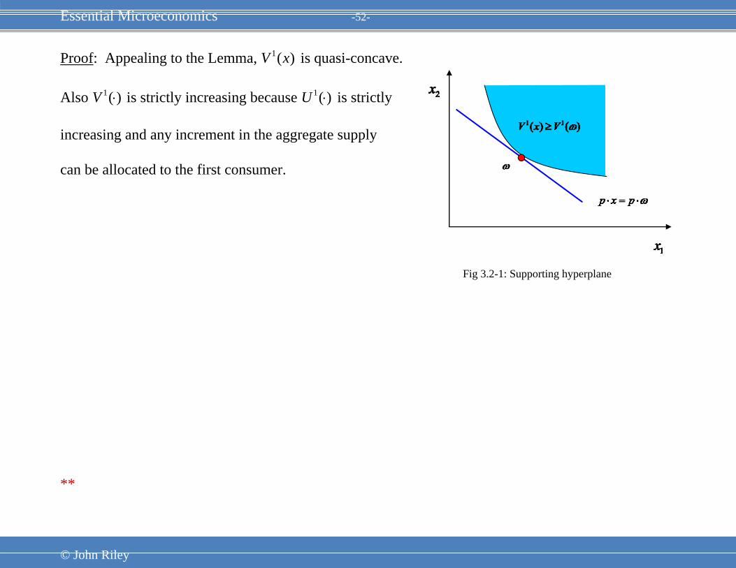
Proof: Appealing to the Lemma, 1( )V x is quasi-concave.

Also 1( )V ⋅ is strictly increasing because 1( )U ⋅ is strictly

increasing and any increment in the aggregate supply

can be allocated to the first consumer.

**

Fig 3.2-1: Supporting hyperplane


© John Riley





An indifference curve for 1( )V ⋅ is depicted.

As we have noted that ˆ{ }hhx ∈H solves ( )PE x

if x ω= .

Moreover, because 1( )U ⋅ is strictly increasing,

1

ˆH

h

h

x ω=

=∑ . (3.2-2)

*



© John Riley





An indifference curve for 1( )V ⋅ is depicted.

As we have noted that ˆ{ }hhx ∈H solves ( )PE x

if x ω= .

Moreover, because 1( )U ⋅ is strictly increasing,

1

ˆH

h

h

x ω=

=∑ . (3.2-2)

Because ω is on the boundary of the upper contour set 1 1{ | ( ) ( )}x V x V ω≥ , it follows from the

Supporting Hyperplane Theorem that there is a vector 0p ≠ , such that all the points in the upper

contour set lie in the set { | }x p x p ω⋅ ≥ ⋅



© John Riley

Formally,

1 1 1 1( ) ( ) and ( ) ( )V x V p x p V x V p x pω ω ω ω> ⇒ ⋅ > ⋅ ≥ ⇒ ⋅ ≥ ⋅ . (3.2-3)

We now argue that the vector p must be positive.

If not, define 1( ,..., ) 0nδ δ δ= > such that

0jδ > if and only if 0jp < .

Then 1 1( ) ( )V Vω δ ω+ > and ( )p pω δ ω⋅ + < ⋅ .

But this contradicts (3.2-3) so p must be positive after all.



© John Riley

To complete the proof we appeal to (3.2-1) - (3.2-3).

1

1 1 1

{ } 1

ˆ( ) { ( ) | ( ) ( ), 2,..., , 0}h H

h

Hh h h h h

x hV x Max U x U x U x h H x x

= =

= ≥ = − ≥∑

(3.2-1)

1

ˆH

h

hx ω

=

=∑ (3.2-2)


From (3.2-3)

1

ˆ( ) ( ), 1,...,H

h h h h h

hU x U x h H p x p x p ω

=

≥ = ⇒ ⋅ = ⋅ ≥ ⋅∑ . (3.2-4)

*


© John Riley

To complete the proof we appeal to (3.2-1) - (3.2-3).

1

1 1 1

{ } 1

ˆ( ) { ( ) | ( ) ( ), 2,..., , 0}h H

h

Hh h h h h

x hV x Max U x U x U x h H x x

= =

= ≥ = − ≥∑

(3.2-1)

1

ˆH

h

hx ω

=

=∑ (3.2-2)


From (3.2-3)

1

ˆ( ) ( ), 1,...,H

h h h h h

hU x U x h H p x p x p ω

=

≥ = ⇒ ⋅ = ⋅ ≥ ⋅∑ . (3.2-5)

Substituting for ω from (3.2-2) it follows that

1 1

ˆ ˆ( ) ( ), 1,...,H H

h h h h h h

h hU x U x h H p x p x

= =

≥ = ⇒ ⋅ ≥ ⋅∑ ∑ .

Setting ˆ ,k kx x k h= ≠ , we may then conclude that for consumer h,

ˆ ˆ( ) ( )h h h h h hU x U x p x p x≥ ⇒ ⋅ ≥ ⋅ .


© John Riley

It remains to show that any strictly preferred bundle costs strictly more.

Suppose instead that ˆ ˆ( ) ( ) andh h h h h hU x U x p x p x> ⋅ = ⋅ .

Then for all (0,1)λ∈ , ˆh hp x p xλ⋅ < ⋅ .

Also because ( )hU ⋅ is continuous, for all λ sufficiently close to 1,

ˆ( ) ( )h h h hU x U xλ > .

But this cannot be true since we have just shown that

ˆ ˆ( ) ( )h h h h h hU x U x p x p x≥ ⇒ ⋅ ≥ ⋅

Hence

ˆ ˆ( ) ( )h h h h h hU x U x p x p x> ⇒ ⋅ > ⋅ .

Q.E.D.

Documents

3. THE EXCHANGE ECONOMY - Essential …essentialmicroeconomics.com/ChapterY3/SlideChapter3.pdf · 3. THE EXCHANGE ECONOMY ... If preferences are CES with elasticity of substitution