Embed Size (px)
Citation preview

3 Ways to Improve Your Regression:Part 2
January 27, 2016
Outline
• Quick review of Part 1o Concepts covered
o Results
• Nonlinear regression splineso Reading basis function code
o Plotting
o Including interactions
• Stochastic gradient boostingo Interaction control language
o Partial dependency plots
o Spline approximation
• Case studies and other applications
• Questions
Salford Systems © 2016 2
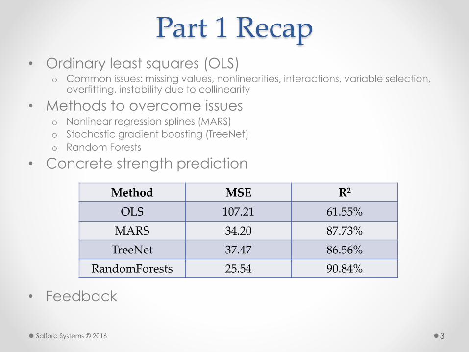
Part 1 Recap• Ordinary least squares (OLS)
o Common issues: missing values, nonlinearities, interactions, variable selection, overfitting, instability due to collinearity
• Methods to overcome issueso Nonlinear regression splines (MARS)
o Stochastic gradient boosting (TreeNet)
o Random Forests
• Concrete strength prediction
• Feedback
Salford Systems © 2016 3
Method MSE R2
OLS 107.21 61.55%
MARS 34.20 87.73%
TreeNet 37.47 86.56%
RandomForests 25.54 90.84%

Nonlinear Regression Splines
• Uses “knots” to impose local linearities
• These knots create “basis functions” to decompose
the information in each variable individually
• Can also perform well on binary dependent variables
• MARS (Multivariate Adaptive Regression Splines)
0
10
20
30
40
50
60
0 10 20 30 40
LSTAT
MV
-10
0
10
20
30
40
50
60
0 10 20 30 40
LSTAT
MV
Salford Systems © 2016 4
Modeling Process
Salford Systems © 2016 5
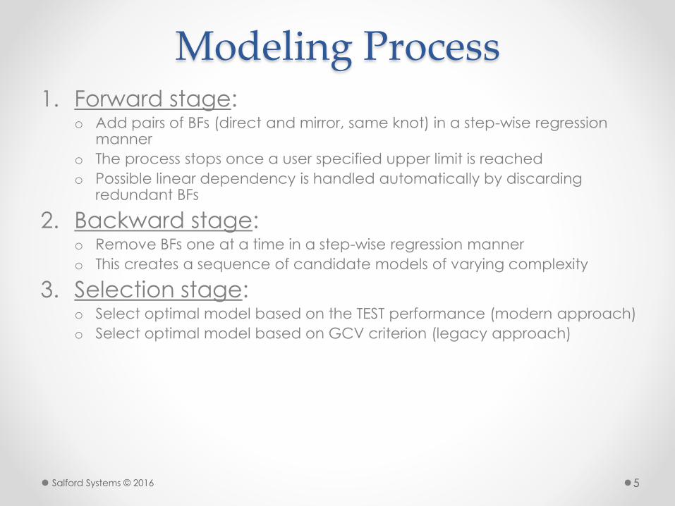
1. Forward stage:o Add pairs of BFs (direct and mirror, same knot) in a step-wise regression
manner
o The process stops once a user specified upper limit is reached
o Possible linear dependency is handled automatically by discarding redundant BFs
2. Backward stage:o Remove BFs one at a time in a step-wise regression manner
o This creates a sequence of candidate models of varying complexity
3. Selection stage:o Select optimal model based on the TEST performance (modern approach)
o Select optimal model based on GCV criterion (legacy approach)

Basis Functions Code
Salford Systems © 2016 6
• Basis Functions (BF) provide analytical machinery to express knots:o Direct: max (0, X -c)
o Mirror: max (0, c - X)
o This is a continuous transformation of variable X into X*
o Value ‘c’ defines the knot placement and constructed for any data value
BF1 = max( 0, AGE - 56);
BF2 = max( 0, 56 - AGE);
BF3 = max( 0, CEMENT - 531.3);
BF4 = max( 0, 531.3 - CEMENT);
BF5 = max( 0, BLAST_FURNACE_SLAG - 19);
Y = 211.582 + 1.5734 * BF1 - 1.9215 * BF2 + 0.998637 * BF3
+ 0.078569 * BF4 + 0.26698 * BF5;
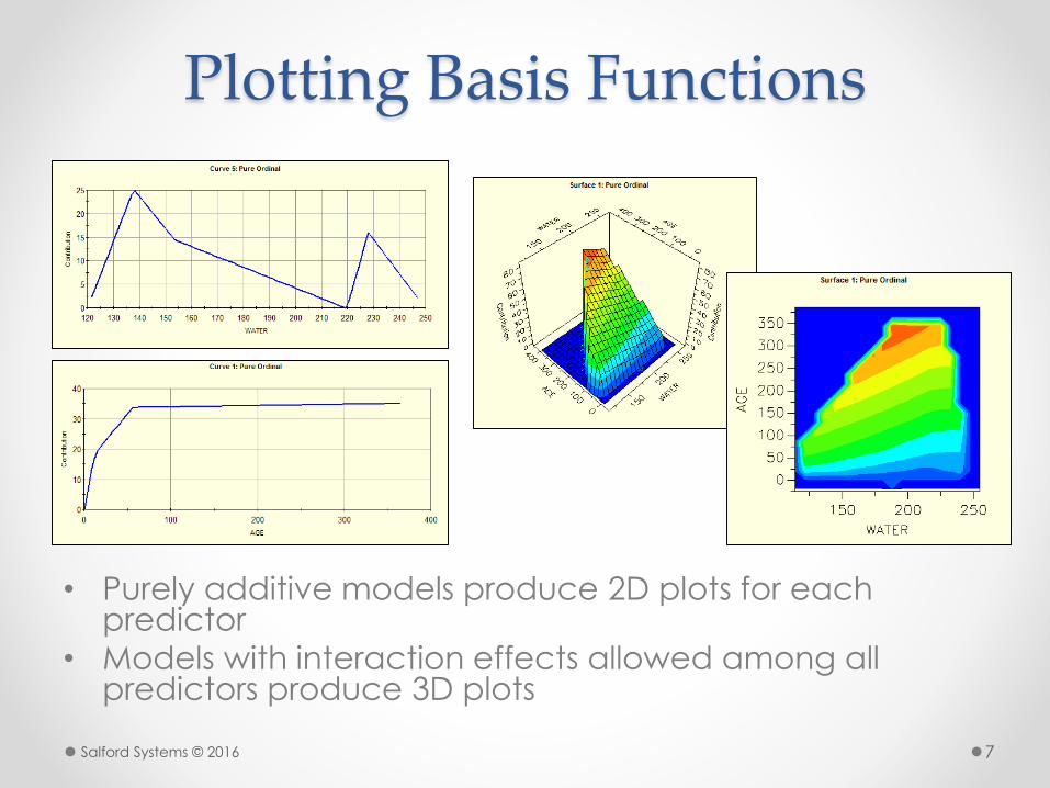
Plotting Basis Functions
• Purely additive models produce 2D plots for each predictor
• Models with interaction effects allowed among all predictors produce 3D plots
Salford Systems © 2016 7

Including Interactions
Salford Systems © 2016 8
• Until now we have considered only ADDITIVE entry of basis functions
• Optionally, MARS will test an interaction with candidate basis function pairo Identify a candidate pair of basis functions
o Test contribution when added to model as standalone
o Test contribution when interacted with basis functions already in model
• Interactions are thus built by accretiono One of the members of the interaction must appear as a main effect
o Then an interaction can be created involving this term
o The second member of the interaction does NOT need to enter as a main effect
• Generally a MARS interaction is region specifico i.e. (PT - 18.6)+ * (RM - 6.431)+
• This is not the familiar interaction of PT*RM because the interaction is
confined to the data region where RM>6.431 and PT>18.6
• MARS could construct a different interaction outside of this region
• Recommended that modeler try a series of models (AUTOMATE)o additive
o 2-way interactions
o 3-way interactions
o 4-way interactions, etc.
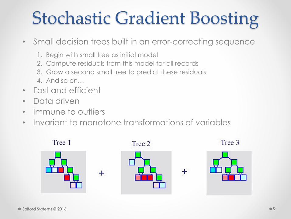
Stochastic Gradient Boosting• Small decision trees built in an error-correcting sequence
1. Begin with small tree as initial model
2. Compute residuals from this model for all records
3. Grow a second small tree to predict these residuals
4. And so on…
• Fast and efficient
• Data driven
• Immune to outliers
• Invariant to monotone transformations of variables
Salford Systems © 2016 9
Interaction Control• TreeNet models are always additive in trees
• Interactions may only enter at the individual tree
level
• Larger trees allow more opportunities for
interactionso 2-node trees force additive models
o 3-node trees allow pair-wise interactions only
o The degree of interactions relates to the number of levels in the tree
• TN can generate a special report with estimates of
interactions in the model
• TN offers additional model building flexibility by
allowing direct control over which variables are
allowed to interact and to what degree
Salford Systems © 2016 10
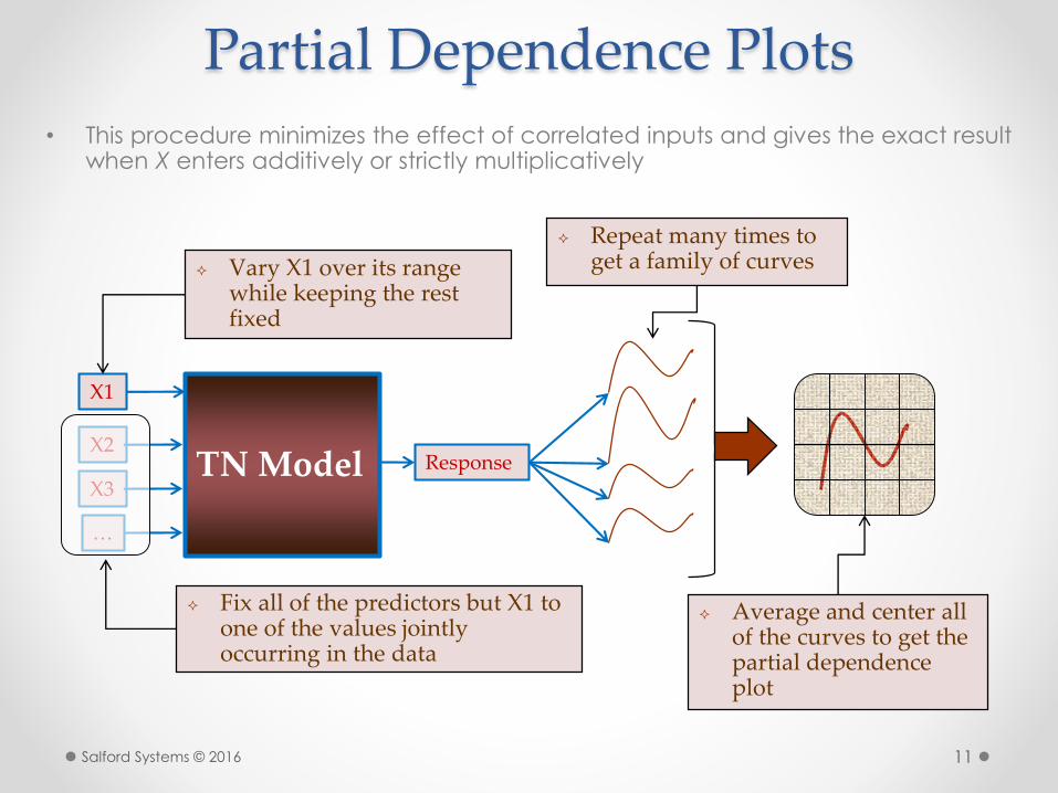
Partial Dependence Plots• This procedure minimizes the effect of correlated inputs and gives the exact result
when X enters additively or strictly multiplicatively
TN Model
X1
X2
X3
…
Response
Fix all of the predictors but X1 to one of the values jointly occurring in the data
Vary X1 over its range while keeping the rest fixed
Repeat many times to get a family of curves
Average and center all of the curves to get the partial dependence plot
11Salford Systems © 2016
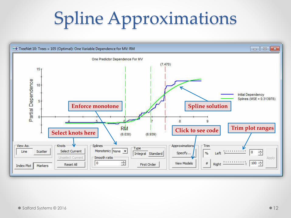
Spline Approximations
Salford Systems © 2016 12
Select knots here Click to see code
Spline solutionEnforce monotone
Trim plot ranges
Model Automation
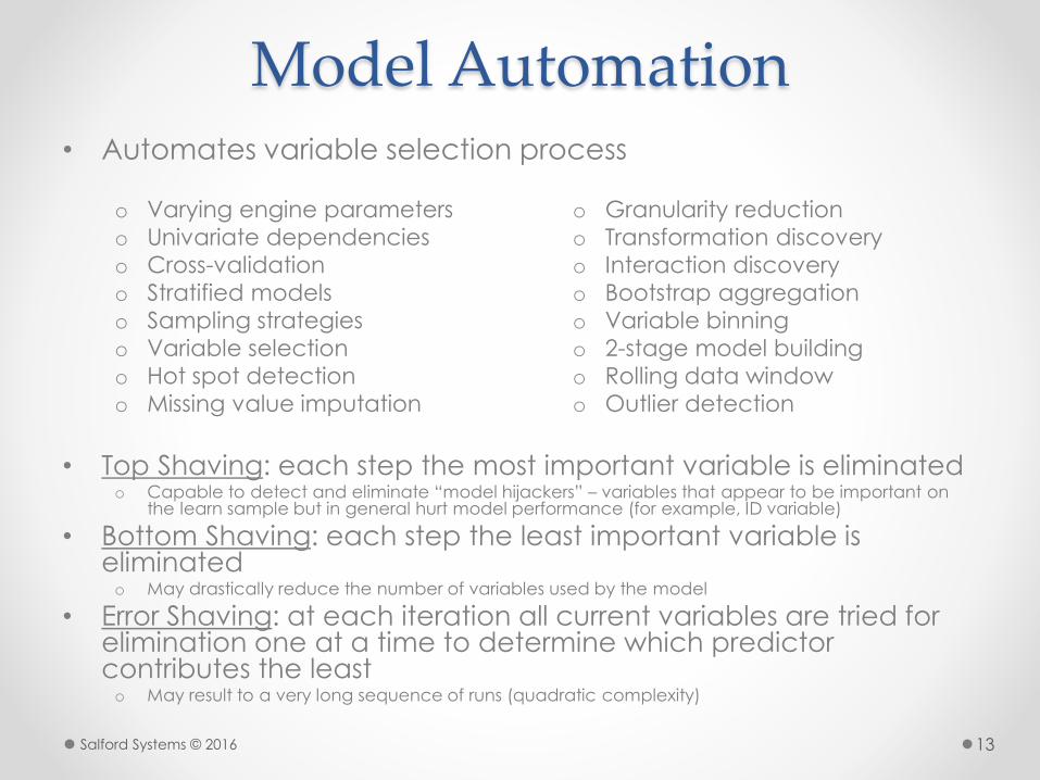
• Top Shaving: each step the most important variable is eliminatedo Capable to detect and eliminate “model hijackers” – variables that appear to be important on
the learn sample but in general hurt model performance (for example, ID variable)
• Bottom Shaving: each step the least important variable is eliminatedo May drastically reduce the number of variables used by the model
• Error Shaving: at each iteration all current variables are tried for elimination one at a time to determine which predictor contributes the leasto May result to a very long sequence of runs (quadratic complexity)
Salford Systems © 2016 13
o Varying engine parameters
o Univariate dependencies
o Cross-validation
o Stratified models
o Sampling strategies
o Variable selection
o Hot spot detection
o Missing value imputation
o Granularity reduction
o Transformation discovery
o Interaction discovery
o Bootstrap aggregation
o Variable binning
o 2-stage model building
o Rolling data window
o Outlier detection
• Automates variable selection process
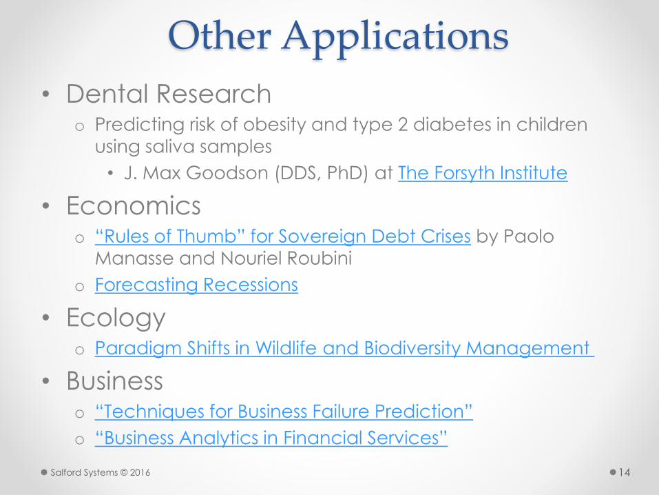
Other Applications
• Dental Researcho Predicting risk of obesity and type 2 diabetes in children
using saliva samples
• J. Max Goodson (DDS, PhD) at The Forsyth Institute
• Economicso “Rules of Thumb” for Sovereign Debt Crises by Paolo
Manasse and Nouriel Roubini
o Forecasting Recessions
• Ecologyo Paradigm Shifts in Wildlife and Biodiversity Management
• Businesso “Techniques for Business Failure Prediction”
o “Business Analytics in Financial Services”
Salford Systems © 2016 14

• Epidemiologyo Relationship between vitamin E levels and myocardial
infarction
o Is coronary calcification associated with regional left
ventricular dysfunction?
• Healthcareo “Identifying Key Determinates of Quality in Health Care”
o “Applied Multivariable Modeling in Public Health”
• Social Scienceso Analyzing RMV data to determine the extent of racial and
gender profiling
o Profiling Poverty with Multivariate Adaptive Regression
Splines
Salford Systems © 2016 15
More Applications

Questions?
• Follow-up email:o Recording of webinar
o PowerPoint slides
o SPM 30-day trial download instructions
o Tutorial with concrete dataset
Salford Systems © 2016 16