Embed Size (px)
Citation preview
3.1
3.0 Area of Review and Corrective Action Plan
This chapter describes how site geologic and hydrologic information were used to delineate the Area of Review (AoR) as it is defined in 40 CFR 146.84(a). This chapter also addresses the extent to which the Alliance needs to undertake corrective actions for features within the AoR that may penetrate the confining zone and how such corrective actions will be taken if needed in the future. Section 3.1 describes the computational model that was used to delineate the AoR, including a description of the simulator and the physical processes modeled, along with a description of the conceptual model and numerical implementation. It also describes the AoR and how the AoR will be reevaluated over time. Section 3.2 describes the Alliance’s corrective action plan. Chapter 3.0 is intended to demonstrate compliance with 40 CFR 146.84.
3.1 Area of Review
The EPA GS Rule (75 FR 77230) defines the AoR as “the region surrounding the geologic sequestration project where underground sources of drinking water (USDWs) may be endangered by the injection activity” (40 CFR 146.84). Section 3.1.8 describes delineation of the proposed AoR for the Morgan County CO2 storage site. All requested data (wells, cleanup sites, surface bodies of water, structures intended for human occupancy, etc.) for this area are provided in this application; the same information is also provided for a larger survey area of 25 mi2 to demonstrate conclusively that USDWs will not be endangered by injection activities.
As discussed in Section 2.6, the natural ambient hydraulic head conditions within the proposed injection zone beneath the Morgan County storage site are higher than the hydraulic head conditions measured in the lowermost USDW (St. Peter Formation) of the stratigraphic well. The EPA suggests using a methodology for determining the AoR based either on the maximum extent of the separate-phase plume, or on the maximum extent of the pressure front, whichever is greater. Because the injection zone is overpressured relative to the lowermost USDW at the Morgan County storage site, use of the pressure front methodology would result in an infinite AoR. Therefore, the maximum extent of the separate-phase plume will be the basis for the AoR delineation for the Morgan County site. A discussion of this AoR delineation, and the measures that are being taken to ensure that the FutureGen 2.0 Project is protective of USDW aquifers, is provided in Section 3.1.9.
The GS Rule requires that the AoR “is delineated using computational modeling that accounts for the physical and chemical properties of all phases of the injected carbon dioxide stream and displaced fluids, and is based on available site characterization, monitoring, and operational data” (40 CFR 146.84). Computational modeling comprises two elements: a computer code, or simulator, that implements the mathematics of our scientific understanding, and implementation of the simulator as an analytical tool. These elements result in the ability to predict the quantity and distribution of CO2 injected into saline reservoirs for storage. This requires solving the mathematical equations that describe the migration and partition behavior of supercritical CO2 (scCO2) as it is injected into geologic media for which the pore space is initially filled with an aqueous saline solution (brine). The equations that describe these flow and transport processes are too complex to solve directly. Therefore, the governing flow and transport equations are solved indirectly where space and time are divided into discrete elements. Space discretization involves dividing the reservoir into grid blocks and time discretization involves moving through time using finite steps. The discretization process transforms the governing flow and transport
3.2
equations into forms that are solvable on high-speed computers. Both elements of the computational model used to determine the AoR for the Morgan County CO2 storage site are described in the sections that follow.
3.1.1 Description of Simulator
Numerical simulation of CO2 injection into deep geologic reservoirs requires the modeling of complex, coupled hydrologic, chemical, and thermal processes, including multi-fluid flow and transport, partitioning of CO2 into the aqueous phase, and chemical interactions with aqueous fluids and rock minerals. The simulations conducted for this investigation were executed using the STOMP-CO2 simulator (White et al. 2012; White and Oostrom 2006; White and Oostrom 2000). STOMP-CO2 was verified against other codes used for simulation of geologic disposal of CO2 as part of the GeoSeq code intercomparison study (Pruess et al. 2002).
Partial differential conservation equations for fluid mass, energy, and salt mass compose the fundamental equations for STOMP-CO2. Coefficients within the fundamental equations are related to the primary variables through a set of constitutive relationships. The salt transport equations are solved simultaneously with the component mass and energy conservation equations. The solute and reactive species transport equations are solved sequentially after the coupled flow and transport equations. The fundamental coupled flow equations are solved using an integral volume finite-difference approach with the nonlinearities in the discretized equations resolved through Newton-Raphson iteration. The dominant nonlinear functions within the STOMP-CO2 simulator are the relative permeability-saturation-capillary pressure (k-s-p) relationships.
The STOMP-CO2 simulator allows the user to specify these relationships through a large variety of popular and classic functions. Two-phase (gas-aqueous) k-s-p relationships can be specified with hysteretic or nonhysteretic functions or nonhysteretic tabular data. Entrapment of CO2 with imbibing water conditions can be modeled with the hysteretic two-phase k-s-p functions. Two-phase k-s-p relationships span both saturated and unsaturated conditions. The aqueous phase is assumed to never completely disappear through extensions to the s-p function below the residual saturation and a vapor-pressure lowering scheme. Supercritical CO2 has the function of a gas in these two-phase k-s-p relationships.
For the range of temperature and pressure conditions present in deep saline reservoirs, four phases are possible: 1) water-rich liquid (aqueous), 2) CO2-rich vapor (gas), 3) CO2-rich liquid (liquid-CO2), and 4) crystalline salt (precipitated salt). The equations of state express 1) the existence of phases given the temperature, pressure, and water, CO2, and salt concentration; 2) the partitioning of components among existing phases; and 3) the density of the existing phases. Thermodynamic properties for CO2 are computed via interpolation from a property data table stored in an external file. The property table was developed from the equation of state for CO2 published by Span and Wagner (1996). Phase equilibria calculations in STOMP-CO2 use the formulations of Spycher et al. (2003) for temperatures below 100°C and Spycher and Pruess (2010) for temperatures above 100°C, with corrections for dissolved salt provided in Spycher and Pruess (2010). The Spycher formulations are based on the Redlich-Kwong equation of state with parameters fitted from published experimental data for CO2-H2O systems. Additional details regarding the equations of state used in STOMP-CO2 can be found in the guide by White et al. (2012).
3.3
A well model is defined as a type of source term that extends over multiple grid cells, where the well diameter is smaller than the grid cell. A fully coupled well model in STOMP-CO2 was used to simulate the injection of scCO2 under a specified mass injection rate, subject to a pressure limit. When the mass injection rate can be met without exceeding the specified pressure limit, the well is considered to be flow controlled. Conversely, when the mass injection rate cannot be met without exceeding the specified pressure limit, the well is considered to be pressure controlled and the mass injection rate is determined based on the injection pressure. The well model assumes a constant pressure gradient within the well and calculates the injection pressure at each cell in the well. The CO2 injection rate is proportional to the pressure gradient between the well and surrounding formation in each grid cell. By fully integrating the well equations into the reservoir field equations, the numerical convergence of the nonlinear conservation and constitutive equations is greatly enhanced.
3.1.2 Physical Processes Modeled
Physical processes modeled in the reservoir simulations included isothermal multi-fluid flow and transport for a number of components (e.g., water, salt, and CO2) and phases (e.g., aqueous and gas). Isothermal conditions were modeled because it was assumed that the temperature of the injected CO2 will be similar to the formation temperature. Reservoir salinity is considered in the simulations because salt precipitation can occur near the injection well in higher permeability layers as the rock dries out during CO2 injection. This can completely plug pore throats, making the layer impermeable, thereby reducing reservoir injectivity and affecting the distribution of CO2 in the reservoir.
Injected CO2 partitions in the reservoir between the free (or mobile) gas, entrapped gas, and aqueous phases. Sequestering CO2 in deep saline reservoirs occurs through four mechanisms: 1) structural trapping, 2) aqueous dissolution, 3) hydraulic trapping, and 4) mineralization. Structural trapping is the long-term retention of the buoyant gas phase in the pore space of the reservoir rock held beneath one or more impermeable caprocks. Aqueous dissolution occurs when CO2 dissolves in the brine resulting in an aqueous-phase density greater than the ambient conditions. Hydraulic trapping is the pinch-off trapping of the gas phase in pores as the brine re-enters pore spaces previously occupied by the gas phase. Generally, hydraulic trapping only occurs upon the cessation of CO2 injection. Mineralization is the chemical reaction that transforms formation minerals to carbonate minerals. In the Mount Simon Sandstone, the most likely precipitation reaction is the formation of iron carbonate precipitates. A likely reaction between CO2 and shale is the dewatering of clays. Laboratory investigations are currently quantifying the importance of these reactions at the Morgan County CO2 storage site. Therefore, the simulations described here did not include mineralization reactions. However, the STOMP-CO2 simulator does account for precipitation of salt during CO2 injection.
The CO2 stream provided by the plant to the storage site is no less than 97 percent dry basis CO2, (see Table 4.1 in Chapter 4.0). Because the amount of impurities is small, for the purposes of modeling the CO2 injection and redistribution for this project, it was assumed that the injectate was pure CO2.
3.1.3 Conceptual Model
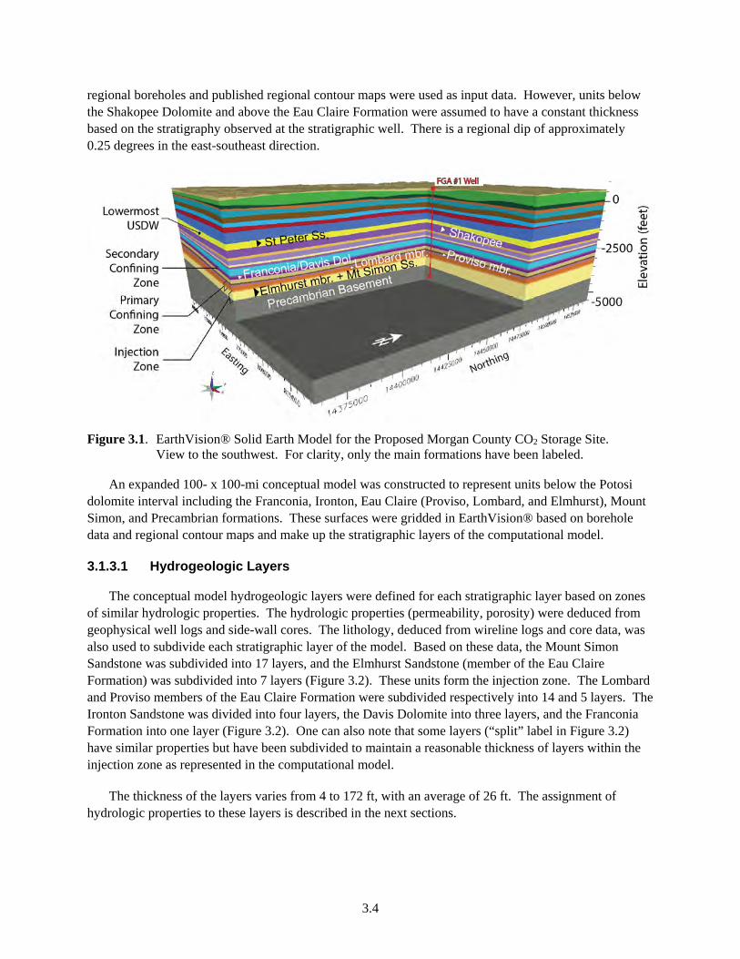
A stratigraphic conceptual model of the geologic layers from the Precambrian basement to ground surface was constructed using the EarthVision® software package (Figure 3.1). The geologic setting and site characterization data described in Chapter 2.0 and later in this chapter were the basis for the Morgan County CO2 storage site model. Borehole data from the FutureGen 2.0 stratigraphic well and data from
3.4
regional boreholes and published regional contour maps were used as input data. However, units below the Shakopee Dolomite and above the Eau Claire Formation were assumed to have a constant thickness based on the stratigraphy observed at the stratigraphic well. There is a regional dip of approximately 0.25 degrees in the east-southeast direction.
Figure 3.1. EarthVision® Solid Earth Model for the Proposed Morgan County CO2 Storage Site. View to the southwest. For clarity, only the main formations have been labeled.
An expanded 100- x 100-mi conceptual model was constructed to represent units below the Potosi dolomite interval including the Franconia, Ironton, Eau Claire (Proviso, Lombard, and Elmhurst), Mount Simon, and Precambrian formations. These surfaces were gridded in EarthVision® based on borehole data and regional contour maps and make up the stratigraphic layers of the computational model.
3.1.3.1 Hydrogeologic Layers
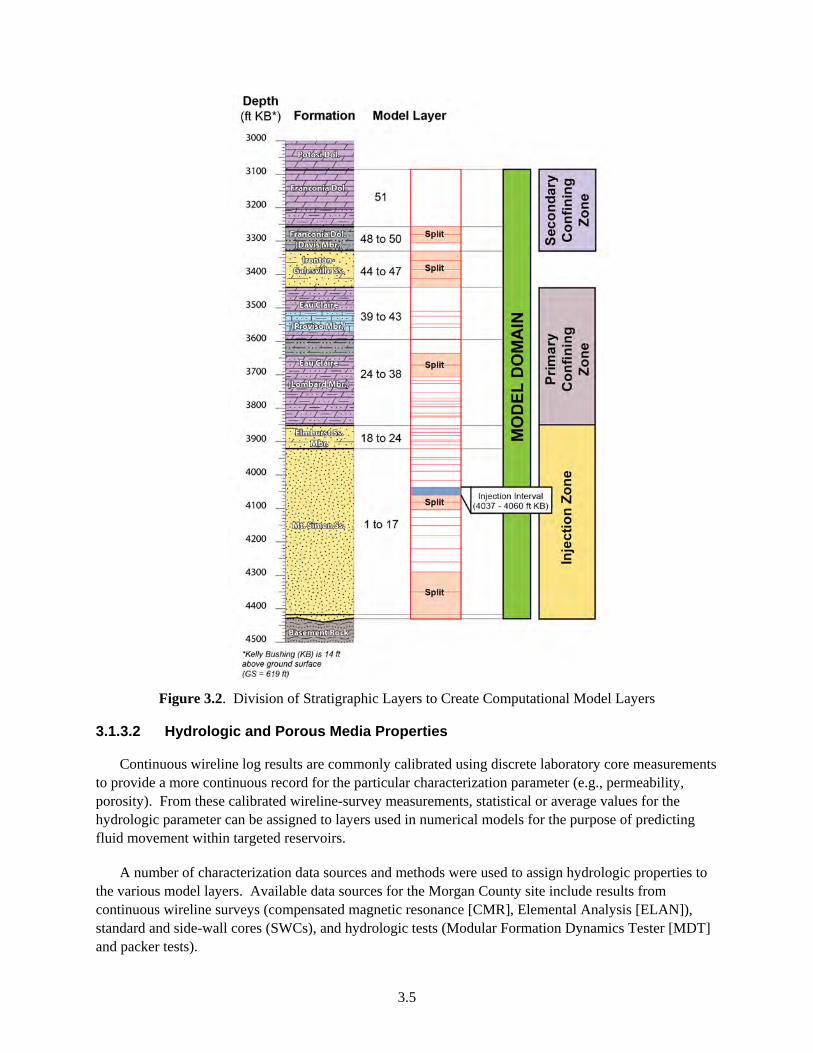
The conceptual model hydrogeologic layers were defined for each stratigraphic layer based on zones of similar hydrologic properties. The hydrologic properties (permeability, porosity) were deduced from geophysical well logs and side-wall cores. The lithology, deduced from wireline logs and core data, was also used to subdivide each stratigraphic layer of the model. Based on these data, the Mount Simon Sandstone was subdivided into 17 layers, and the Elmhurst Sandstone (member of the Eau Claire Formation) was subdivided into 7 layers (Figure 3.2). These units form the injection zone. The Lombard and Proviso members of the Eau Claire Formation were subdivided respectively into 14 and 5 layers. The Ironton Sandstone was divided into four layers, the Davis Dolomite into three layers, and the Franconia Formation into one layer (Figure 3.2). One can also note that some layers (“split” label in Figure 3.2) have similar properties but have been subdivided to maintain a reasonable thickness of layers within the injection zone as represented in the computational model.
The thickness of the layers varies from 4 to 172 ft, with an average of 26 ft. The assignment of hydrologic properties to these layers is described in the next sections.
3.5
Figure 3.2. Division of Stratigraphic Layers to Create Computational Model Layers
3.1.3.2 Hydrologic and Porous Media Properties
Continuous wireline log results are commonly calibrated using discrete laboratory core measurements to provide a more continuous record for the particular characterization parameter (e.g., permeability, porosity). From these calibrated wireline-survey measurements, statistical or average values for the hydrologic parameter can be assigned to layers used in numerical models for the purpose of predicting fluid movement within targeted reservoirs.
A number of characterization data sources and methods were used to assign hydrologic properties to the various model layers. Available data sources for the Morgan County site include results from continuous wireline surveys (compensated magnetic resonance [CMR], Elemental Analysis [ELAN]), standard and side-wall cores (SWCs), and hydrologic tests (Modular Formation Dynamics Tester [MDT] and packer tests).

3.6
Because of differences in lithology and in the borehole construction, the method used to assign properties varied for different vertical zones of the conceptual model.
Horizontal Permeability
Intrinsic permeability is the property of the rock/formation that relates to its ability to transmit fluid, and is independent of the in situ fluid properties. For modeling of sedimentary rock formations, two permeabilities are commonly used: permeability in the horizontal direction, kh (permeability parallel to sedimentary layering [also Kh]) and permeability in the vertical direction, kv (permeability perpendicular to layering [also Kv]). The subsequent discussion pertains to assigned horizontal permeability values for the various borehole sections.
Intrinsic permeability data sources for the FutureGen 2.0 stratigraphic well include computed geophysical wireline surveys (CMR and ELAN logs), and where available, laboratory measurements of rotary SWCs, core plugs from the whole core intervals, and hydrologic tests (including wireline [MDT]), and packer tests.
Intrinsic Permeability in the Injection Zone (Mount Simon and Elmhurst Sandstone)
For model layers within the injection reservoir section (i.e., Elmhurst Sandstone and Mount Simon Sandstone; 3,852 to 4,432 ft [1174 to 1350 m]) a correlation/calibration approach was applied. Wireline log CMR- and ELAN-computed permeability model responses were first correlated with and then calibrated to rotary side-wall and core plug permeability results. The correlation process was facilitated using natural gamma ray responses and clay or shale abundance to establish correlation data sets. This calibration provided a continuous permeability estimate over the entire injection reservoir section (curve permKCal). The calibrated permeability response was then slightly adjusted, or scaled, to match the composite results obtained from the hydrologic packer tests over uncased intervals. For injection reservoir model layers within the cased well portion of the model, no hydrologic test data are available, and core-calibrated ELAN log response was used directly in assigning average model layer permeabilities.
The hydraulic packer tests were conducted in two zones of the Mount Simon portion of the reservoir. The Upper Zone (3,948 ft bkb to 4,194 ft bkb) equates to layers 6 through 17 of the model, while the Lower Zone (4,200 ft bkb to 4,512 ft bkb) equates to layers 1 through 5.1 The most recent ELAN-based permeability-thickness product values are 9,524 mD-ft for the 246-ft-thick section of the upper Mount Simon corresponding to the Upper Zone and 3,139 mD-ft for the 312-ft-thick section of the lower Mount Simon corresponding to the Lower Zone. The total permeability-thickness product for the open borehole Mount Simon is 12,663 mD-ft, based on the ELAN logs. Results of the field hydraulic tests suggest that the upper Mount Simon permeability-thickness product is 9,040 mD-ft and the lower Mount Simon interval permeability-thickness product is 775 mD-ft. By simple direct comparison, the packer test for the upper Mount Simon is nearly equivalent (~95 percent) to the ELAN-predicted value, while the lower Mount Simon represents only ~25 percent of the ELAN-predicted value (Table 3.1).
1 The layers “MtSimon5” and “MtSimon4” are subdivisions of a single layer. Because the MtSimon5 layer is located between the two testing zones and is more similar in log properties to the lower level, it is assigned as part of the lower zone.
3.7
Because no hydrologic test has been conducted in the Elmhurst Sandstone reservoir interval, a conservative scaling factor of 1 has been assigned to this interval, based on ELAN PermKCal data. The scaling factors applied in the model are listed in Table 3.2.
Table 3.1. Comparison of Results from Hydraulic Field Tests and ELAN Data
Permeability-Thickness Product (mD-ft), T
Tf/Te Field Test, Tf ELAN, Te Upper Mt. Simon 9,040 9,524 0.949 Lower Mt. Simon 775 3,139 0.247
Overall 9,815 12,663 0.775
Table 3.2. Summary of the Scaling Factors Applied for the Modeling
Depth (ft bkb) –
Based on Model Layers Scaling Factor
Caprock and Overburden Formations 3,086 to 3,852 ft 1 Elmhurst 3,852 to 3,922 ft 1
Upper Mt. Simon 3,922 to 4,182 ft 0.949 Lower Mt Simon 4,182 to 4,432 ft 0.247
Intrinsic Permeability in the Confining Zones (Franconia to Lombard Formations)
The sources of data are similar to those for the injection zone reservoir, with the exception that no hydrologic or MDT test data are available.
ELAN log-derived permeabilities are unreliable below about 0.01 mD (personal communication from Bob Butsch, Schlumberger, 2012). Because the average log-derived permeabilities (permKCal wireline from ELAN log) for most of the caprock layers are at or below 0.01 mD, an alternate approach was applied. For each model layer the core data were reviewed, and a simple average of the available horizontal Klinkenburg permeabilities was then calculated for each layer. Core samples that were noted as having potential cracks and/or were very small were eliminated if the results appeared to be unreasonable based on the sampled lithology. If no core samples were available and the arithmetic mean of the PermKCal was below 0.01 mD, a default value of 0.01 mD was applied (Lombard9 is the only layer with a 0.01-mD default value).
Because the sandstone intervals of the Ironton-Galesville Sandstone have higher permeabilities that are similar in magnitude to the modeled reservoir layers, the Ironton-Galesville Sandstone model layer permeabilities were derived from the arithmetic mean of the PermKCal permeability curve.
Because no hydraulic test has been conducted in the primary confining zone, the scaling factor was assigned to be 100 percent in this interval and the overburden formations (Table 3.2).
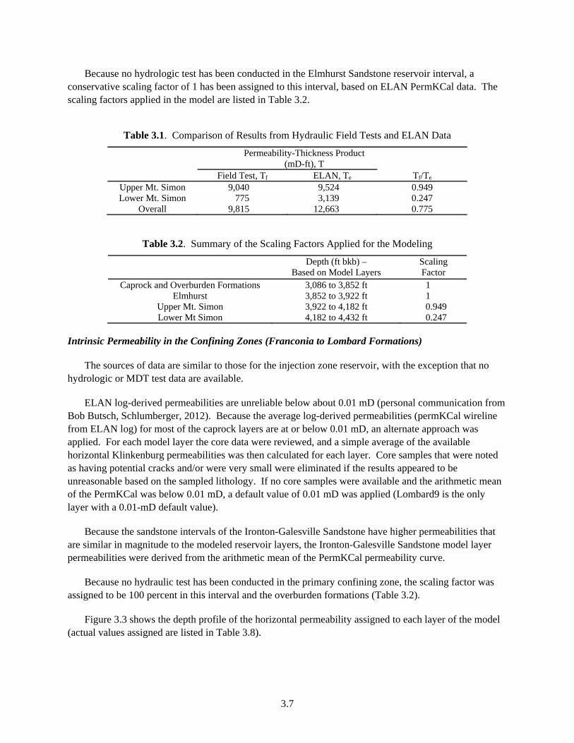
Figure 3.3 shows the depth profile of the horizontal permeability assigned to each layer of the model (actual values assigned are listed in Table 3.8).
3.8
Figure 3.3. Horizontal Permeability Versus Depth in Each Model Layer
Vertical Permeability
Sedimentation can create an intrinsic permeability anisotropy, caused by sediment layering and preferential directions of connected-pore channels. Kv/Kh ratios were successfully determined for 20 vertical/horizontal siliciclastic core plug pairs cut from intervals of whole core from the stratigraphic well. Horizontal permeability data in the stratigraphic well far outnumber vertical permeability data, because vertical permeability could not be determined from rotary SWCs.
Effective vertical permeability in siliciclastic rocks is primarily a function of the presence of mudstone or shale (Ringrose et al. 2005). The siliciclastic lithologies (sandstones, siltstones, mudstones and shales) are heterolithic in the cored interval of the lower Lombard, and in rotary SWCs from the upper Lombard and non-carbonate Proviso. Core plug samples of heterolithic siliciclastics are poorly representative of larger vertical intervals (Meyer and Krause 2006).
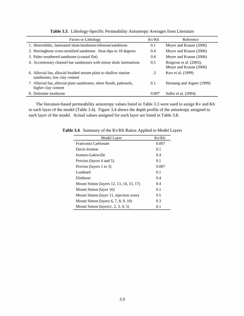
Because the anisotropy of the model layers is not likely to be represented by the sparse data from the stratigraphic well, the following lithology-specific permeability anisotropy averages from literature studies representing larger sample sizes are used for the model layers (Table 3.3).
3.9
Table 3.3. Lithology-Specific Permeability Anisotropy Averages from Literature
Facies or Lithology Kv/Kh Reference
1. Heterolithic, laminated shale/mudstone/siltstone/sandstone 0.1 Meyer and Krause (2006)
2. Herringbone cross-stratified sandstone. Strat dips to 18 degrees 0.4 Meyer and Krause (2006)
3. Paleo weathered sandstone (coastal flat) 0.4 Meyer and Krause (2006)
4. Accretionary channel bar sandstones with minor shale laminations 0.5 Ringrose et al. (2005); Meyer and Krause (2006)
6. Alluvial fan, alluvial braided stream plain to shallow marine sandstones, low clay content
.3 Kerr et al. (1999)
7. Alluvial fan, alluvial plain sandstones, sheet floods, paleosols, higher clay content
0.1 Hornung and Aigner (1999)
8. Dolomite mudstone 0.007 Saller et al. (2004)
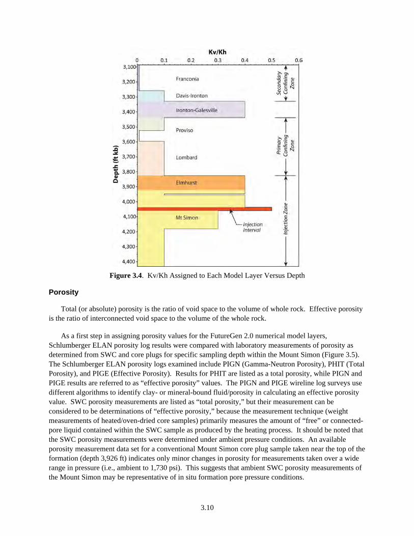
The literature-based permeability anisotropy values listed in Table 3.3 were used to assign Kv and Kh to each layer of the model (Table 3.4). Figure 3.4 shows the depth profile of the anisotropy assigned to each layer of the model. Actual values assigned for each layer are listed in Table 3.8.
Table 3.4. Summary of the Kv/Kh Ratios Applied to Model Layers
Model Layer Kv/Kh
Franconia Carbonate 0.007
Davis-Ironton 0.1
Ironton-Galesville 0.4
Proviso (layers 4 and 5) 0.1
Proviso (layers 1 to 3) 0.007
Lombard 0.1
Elmhurst 0.4
Mount Simon (layers 12, 13, 14, 15, 17) 0.4
Mount Simon (layer 16) 0.1
Mount Simon (layer 11, injection zone) 0.5
Mount Simon (layers 6, 7, 8, 9, 10) 0.3 Mount Simon (layers1, 2, 3, 4, 5) 0.1
3.10
Figure 3.4. Kv/Kh Assigned to Each Model Layer Versus Depth
Porosity
Total (or absolute) porosity is the ratio of void space to the volume of whole rock. Effective porosity is the ratio of interconnected void space to the volume of the whole rock.
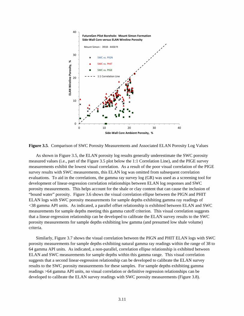
As a first step in assigning porosity values for the FutureGen 2.0 numerical model layers, Schlumberger ELAN porosity log results were compared with laboratory measurements of porosity as determined from SWC and core plugs for specific sampling depth within the Mount Simon (Figure 3.5). The Schlumberger ELAN porosity logs examined include PIGN (Gamma-Neutron Porosity), PHIT (Total Porosity), and PIGE (Effective Porosity). Results for PHIT are listed as a total porosity, while PIGN and PIGE results are referred to as “effective porosity” values. The PIGN and PIGE wireline log surveys use different algorithms to identify clay- or mineral-bound fluid/porosity in calculating an effective porosity value. SWC porosity measurements are listed as “total porosity,” but their measurement can be considered to be determinations of “effective porosity,” because the measurement technique (weight measurements of heated/oven-dried core samples) primarily measures the amount of “free” or connected-pore liquid contained within the SWC sample as produced by the heating process. It should be noted that the SWC porosity measurements were determined under ambient pressure conditions. An available porosity measurement data set for a conventional Mount Simon core plug sample taken near the top of the formation (depth 3,926 ft) indicates only minor changes in porosity for measurements taken over a wide range in pressure (i.e., ambient to 1,730 psi). This suggests that ambient SWC porosity measurements of the Mount Simon may be representative of in situ formation pore pressure conditions.
3.11
Figure 3.5. Comparison of SWC Porosity Measurements and Associated ELAN Porosity Log Values
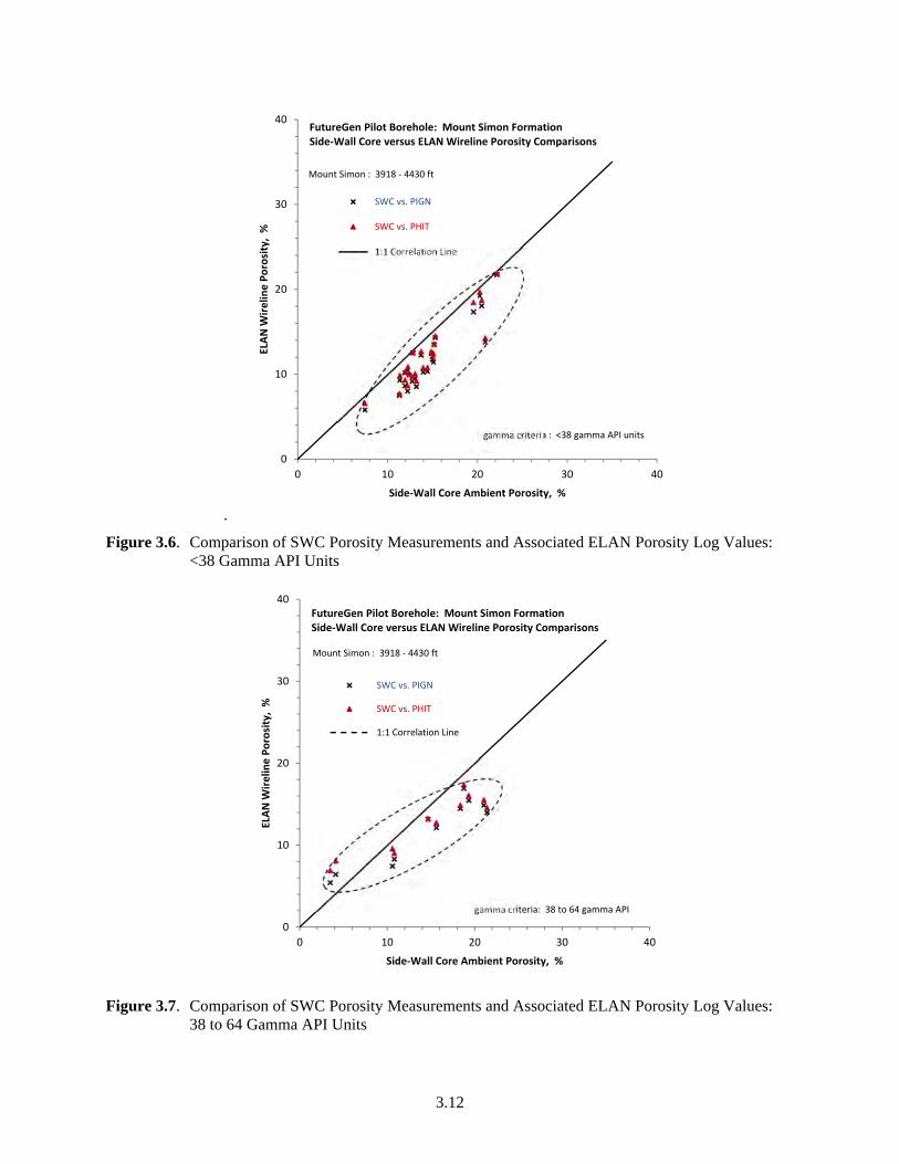
As shown in Figure 3.5, the ELAN porosity log results generally underestimate the SWC porosity measured values (i.e., part of the Figure 3.5 plot below the 1:1 Correlation Line), and the PIGE survey measurements exhibit the lowest visual correlation. As a result of the poor visual correlation of the PIGE survey results with SWC measurements, this ELAN log was omitted from subsequent correlation evaluations. To aid in the correlations, the gamma ray survey log (GR) was used as a screening tool for development of linear-regression correlation relationships between ELAN log responses and SWC porosity measurements. This helps account for the shale or clay content that can cause the inclusion of “bound water” porosity. Figure 3.6 shows the visual correlation ellipse between the PIGN and PHIT ELAN logs with SWC porosity measurements for sample depths exhibiting gamma ray readings of <38 gamma API units. As indicated, a parallel offset relationship is exhibited between ELAN and SWC measurements for sample depths meeting this gamma cutoff criterion. This visual correlation suggests that a linear-regression relationship can be developed to calibrate the ELAN survey results to the SWC porosity measurements for sample depths exhibiting low gamma (and presumed low shale volume) criteria.
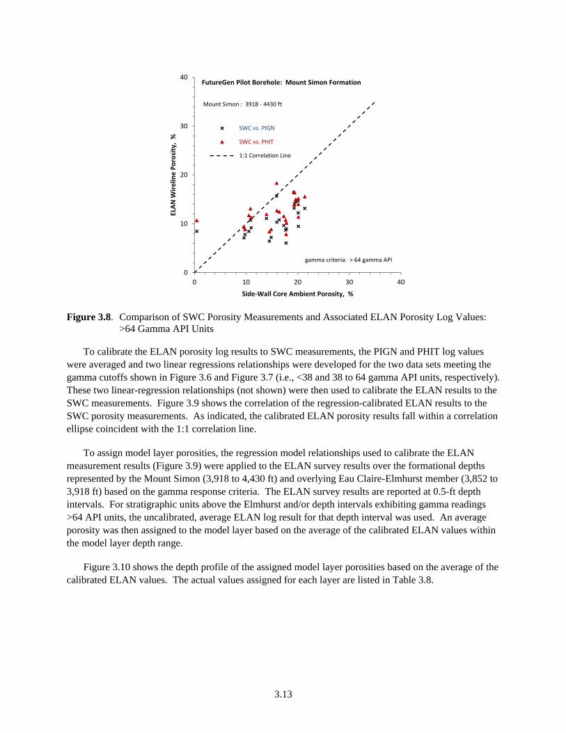
Similarly, Figure 3.7 shows the visual correlation between the PIGN and PHIT ELAN logs with SWC porosity measurements for sample depths exhibiting natural gamma ray readings within the range of 38 to 64 gamma API units. As indicated, a non-parallel, correlation ellipse relationship is exhibited between ELAN and SWC measurements for sample depths within this gamma range. This visual correlation suggests that a second linear-regression relationship can be developed to calibrate the ELAN survey results to the SWC porosity measurements for these samples. For sample depths exhibiting gamma readings >64 gamma API units, no visual correlation or definitive regression relationships can be developed to calibrate the ELAN survey readings with SWC porosity measurements (Figure 3.8).
0
10
20
30
40
0 10 20 30 40
ELAN W
irelin
e Porosity, %
Side‐Wall Core Ambient Porosity, %
SWC vs. PIGN
SWC vs. PHIT
SWC vs. PIGE
1:1 Correlation Line
FutureGen Pilot Borehole: Mount Simon FormationSide‐Wall Core versus ELAN Wireline Porosity
Mount Simon : 3918 ‐ 4430 ft
3.12
.
Figure 3.6. Comparison of SWC Porosity Measurements and Associated ELAN Porosity Log Values: <38 Gamma API Units
Figure 3.7. Comparison of SWC Porosity Measurements and Associated ELAN Porosity Log Values: 38 to 64 Gamma API Units
0
10
20
30
40
0 10 20 30 40
ELAN W
irelin
e Porosity, %
Side‐Wall Core Ambient Porosity, %
SWC vs. PIGN
SWC vs. PHIT
1:1 Correlation Line
FutureGen Pilot Borehole: Mount Simon FormationSide‐Wall Core versus ELAN Wireline Porosity Comparisons
Mount Simon : 3918 ‐ 4430 ft
gamma criteria : <38 gamma API units
0
10
20
30
40
0 10 20 30 40
ELAN W
irelin
e Porosity, %
Side‐Wall Core Ambient Porosity, %
SWC vs. PIGN
SWC vs. PHIT
1:1 Correlation Line
FutureGen Pilot Borehole: Mount Simon FormationSide‐Wall Core versus ELAN Wireline Porosity Comparisons
Mount Simon : 3918 ‐ 4430 ft
gamma criteria: 38 to 64 gamma API
3.13
Figure 3.8. Comparison of SWC Porosity Measurements and Associated ELAN Porosity Log Values: >64 Gamma API Units
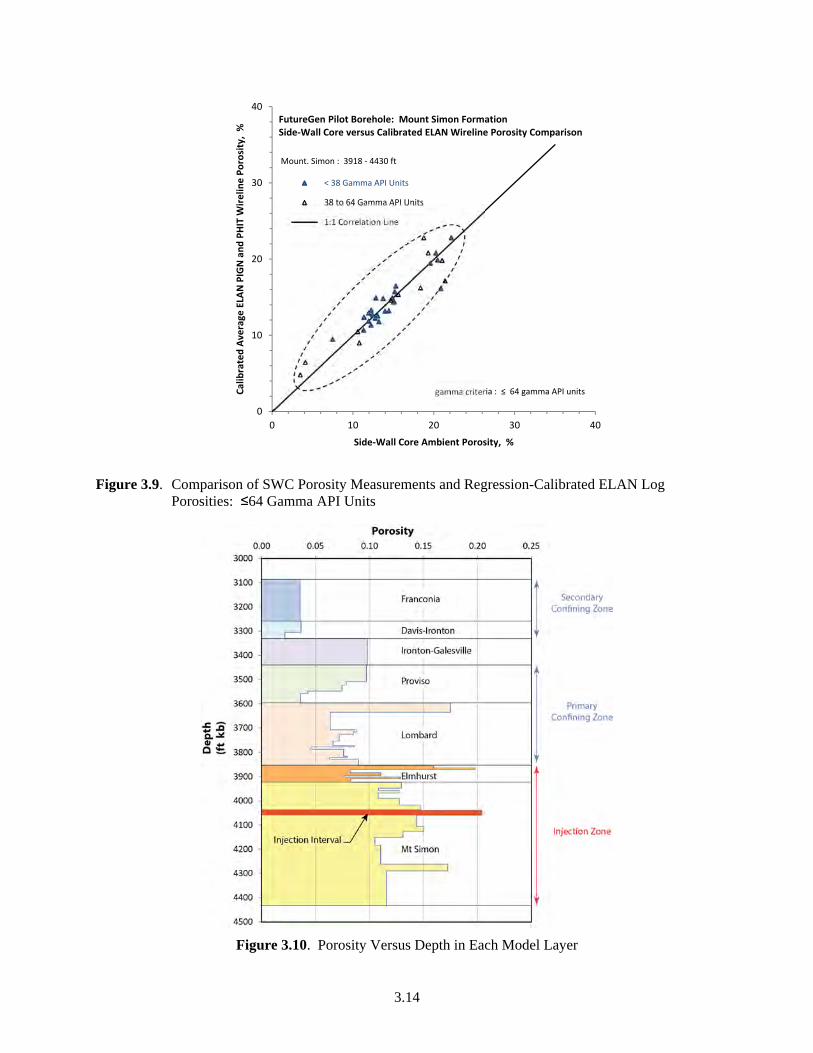
To calibrate the ELAN porosity log results to SWC measurements, the PIGN and PHIT log values were averaged and two linear regressions relationships were developed for the two data sets meeting the gamma cutoffs shown in Figure 3.6 and Figure 3.7 (i.e., <38 and 38 to 64 gamma API units, respectively). These two linear-regression relationships (not shown) were then used to calibrate the ELAN results to the SWC measurements. Figure 3.9 shows the correlation of the regression-calibrated ELAN results to the SWC porosity measurements. As indicated, the calibrated ELAN porosity results fall within a correlation ellipse coincident with the 1:1 correlation line.
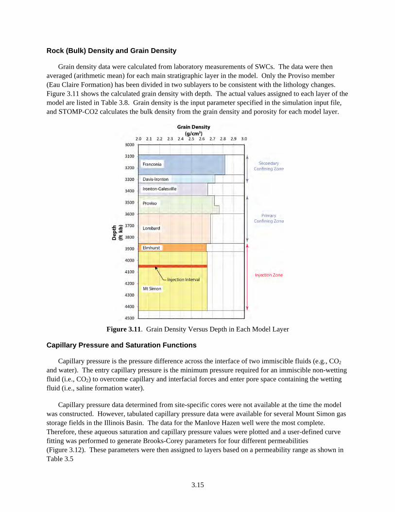
To assign model layer porosities, the regression model relationships used to calibrate the ELAN measurement results (Figure 3.9) were applied to the ELAN survey results over the formational depths represented by the Mount Simon (3,918 to 4,430 ft) and overlying Eau Claire-Elmhurst member (3,852 to 3,918 ft) based on the gamma response criteria. The ELAN survey results are reported at 0.5-ft depth intervals. For stratigraphic units above the Elmhurst and/or depth intervals exhibiting gamma readings >64 API units, the uncalibrated, average ELAN log result for that depth interval was used. An average porosity was then assigned to the model layer based on the average of the calibrated ELAN values within the model layer depth range.
Figure 3.10 shows the depth profile of the assigned model layer porosities based on the average of the calibrated ELAN values. The actual values assigned for each layer are listed in Table 3.8.
0
10
20
30
40
0 10 20 30 40
ELAN W
irelin
e Porosity, %
Side‐Wall Core Ambient Porosity, %
SWC vs. PIGN
SWC vs. PHIT
1:1 Correlation Line
FutureGen Pilot Borehole: Mount Simon Formation
Mount Simon : 3918 ‐ 4430 ft
gamma criteria: > 64 gamma API
3.14
Figure 3.9. Comparison of SWC Porosity Measurements and Regression-Calibrated ELAN Log Porosities: ≤64 Gamma API Units
Figure 3.10. Porosity Versus Depth in Each Model Layer
0
10
20
30
40
0 10 20 30 40
Calibrated Average
ELA
N PIGN and PHIT W
irelin
e Porosity, %
Side‐Wall Core Ambient Porosity, %
< 38 Gamma API Units
38 to 64 Gamma API Units
1:1 Correlation Line
FutureGen Pilot Borehole: Mount Simon FormationSide‐Wall Core versus Calibrated ELAN Wireline Porosity Comparison
Mount. Simon : 3918 ‐ 4430 ft
gamma criteria : ≤ 64 gamma API units
3.15
Rock (Bulk) Density and Grain Density
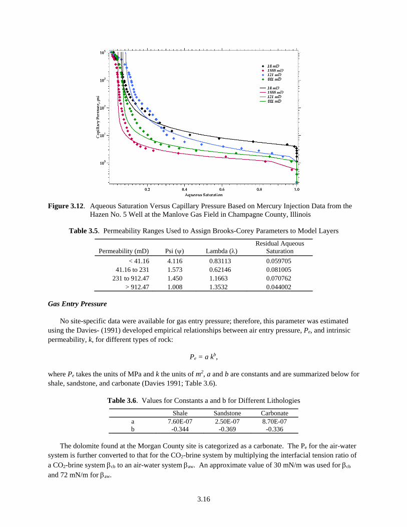
Grain density data were calculated from laboratory measurements of SWCs. The data were then averaged (arithmetic mean) for each main stratigraphic layer in the model. Only the Proviso member (Eau Claire Formation) has been divided in two sublayers to be consistent with the lithology changes. Figure 3.11 shows the calculated grain density with depth. The actual values assigned to each layer of the model are listed in Table 3.8. Grain density is the input parameter specified in the simulation input file, and STOMP-CO2 calculates the bulk density from the grain density and porosity for each model layer.
Figure 3.11. Grain Density Versus Depth in Each Model Layer
Capillary Pressure and Saturation Functions
Capillary pressure is the pressure difference across the interface of two immiscible fluids (e.g., CO2 and water). The entry capillary pressure is the minimum pressure required for an immiscible non-wetting fluid (i.e., CO2) to overcome capillary and interfacial forces and enter pore space containing the wetting fluid (i.e., saline formation water).
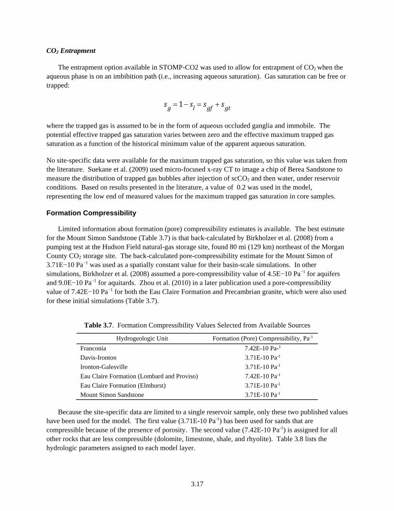
Capillary pressure data determined from site-specific cores were not available at the time the model was constructed. However, tabulated capillary pressure data were available for several Mount Simon gas storage fields in the Illinois Basin. The data for the Manlove Hazen well were the most complete. Therefore, these aqueous saturation and capillary pressure values were plotted and a user-defined curve fitting was performed to generate Brooks-Corey parameters for four different permeabilities (Figure 3.12). These parameters were then assigned to layers based on a permeability range as shown in Table 3.5
3.16
Figure 3.12. Aqueous Saturation Versus Capillary Pressure Based on Mercury Injection Data from the Hazen No. 5 Well at the Manlove Gas Field in Champagne County, Illinois
Table 3.5. Permeability Ranges Used to Assign Brooks-Corey Parameters to Model Layers
Permeability (mD) Psi () Lambda () Residual Aqueous
Saturation
< 41.16 4.116 0.83113 0.059705 41.16 to 231 1.573 0.62146 0.081005
231 to 912.47 1.450 1.1663 0.070762 > 912.47 1.008 1.3532 0.044002
Gas Entry Pressure
No site-specific data were available for gas entry pressure; therefore, this parameter was estimated using the Davies- (1991) developed empirical relationships between air entry pressure, Pe, and intrinsic permeability, k, for different types of rock:
Pe = a kb,
where Pe takes the units of MPa and k the units of m2, a and b are constants and are summarized below for shale, sandstone, and carbonate (Davies 1991; Table 3.6).
Table 3.6. Values for Constants a and b for Different Lithologies
Shale Sandstone Carbonate a 7.60E-07 2.50E-07 8.70E-07 b -0.344 -0.369 -0.336
The dolomite found at the Morgan County site is categorized as a carbonate. The Pe for the air-water system is further converted to that for the CO2-brine system by multiplying the interfacial tension ratio of a CO2-brine system cb to an air-water system aw. An approximate value of 30 mN/m was used for cb and 72 mN/m for aw.
3.17
CO2 Entrapment
The entrapment option available in STOMP-CO2 was used to allow for entrapment of CO2 when the aqueous phase is on an imbibition path (i.e., increasing aqueous saturation). Gas saturation can be free or trapped:
where the trapped gas is assumed to be in the form of aqueous occluded ganglia and immobile. The potential effective trapped gas saturation varies between zero and the effective maximum trapped gas saturation as a function of the historical minimum value of the apparent aqueous saturation.
No site-specific data were available for the maximum trapped gas saturation, so this value was taken from the literature. Suekane et al. (2009) used micro-focused x-ray CT to image a chip of Berea Sandstone to measure the distribution of trapped gas bubbles after injection of scCO2 and then water, under reservoir conditions. Based on results presented in the literature, a value of 0.2 was used in the model, representing the low end of measured values for the maximum trapped gas saturation in core samples.
Formation Compressibility
Limited information about formation (pore) compressibility estimates is available. The best estimate for the Mount Simon Sandstone (Table 3.7) is that back-calculated by Birkholzer et al. (2008) from a pumping test at the Hudson Field natural-gas storage site, found 80 mi (129 km) northeast of the Morgan County CO2 storage site. The back-calculated pore-compressibility estimate for the Mount Simon of 3.71E−10 Pa−1 was used as a spatially constant value for their basin-scale simulations. In other simulations, Birkholzer et al. (2008) assumed a pore-compressibility value of 4.5E−10 Pa−1 for aquifers and 9.0E−10 Pa−1 for aquitards. Zhou et al. (2010) in a later publication used a pore-compressibility value of 7.42E−10 Pa−1 for both the Eau Claire Formation and Precambrian granite, which were also used for these initial simulations (Table 3.7).
Table 3.7. Formation Compressibility Values Selected from Available Sources
Hydrogeologic Unit Formation (Pore) Compressibility, Pa-1
Franconia 7.42E-10 Pa-1
Davis-Ironton 3.71E-10 Pa-1
Ironton-Galesville 3.71E-10 Pa-1
Eau Claire Formation (Lombard and Proviso) 7.42E-10 Pa-1
Eau Claire Formation (Elmhurst) 3.71E-10 Pa-1
Mount Simon Sandstone 3.71E-10 Pa-1
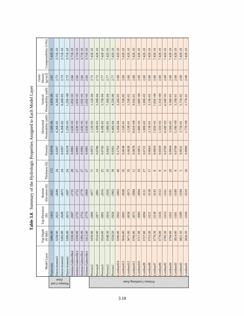
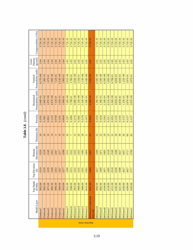
Because the site-specific data are limited to a single reservoir sample, only these two published values have been used for the model. The first value (3.71E-10 Pa-1) has been used for sands that are compressible because of the presence of porosity. The second value (7.42E-10 Pa-1) is assigned for all other rocks that are less compressible (dolomite, limestone, shale, and rhyolite). Table 3.8 lists the hydrologic parameters assigned to each model layer.
sg 1 sl sgf sgt
3.18
Tab
le 3
.8.
Sum
mar
y of
the
Hyd
rolo
gic
Pro
pert
ies
Ass
igne
d to
Eac
h M
odel
Lay
er
Mod
el L
ayer
T
op D
epth
(f
t bkb
) T
op E
leva
tion
(f
t)
Bot
tom
E
leva
tion
(ft
) T
hick
ness
(ft
) P
oros
ity
Hor
izon
tal
Per
mea
bili
ty (
mD
)V
erti
cal
Per
mea
bili
ty (
mD
)
Gra
in
Den
sity
(g
/cm
3)
Com
pres
sibi
lity
(1/
Pa)
Primary Conf. Zone
Fra
ncon
ia
3086
.00
-245
3 -2
625
172
0.03
58
5.50
E-0
6 3.
85E
-08
2.82
7.
42E
-10
Dav
is-I
ront
on3
3258
.00
-262
5 -2
649
24
0.03
67
6.26
E-0
2 6.
26E
-03
2.73
3.
71E
-10
Dav
is-I
ront
on2
3282
.00
-264
9 -2
673
24
0.03
67
6.26
E-0
2 6.
26E
-03
2.73
3.
71E
-10
Dav
is-I
ront
on1
3306
.00
-267
3 -2
697
24
0.02
18
1.25
E+
01
1.25
E+
00
2.73
3.
71E
-10
Ir
onto
n-G
ales
vill
e4
3330
.00
-269
7 -2
725
28
0.09
81
2.63
E+
01
1.05
E+
01
2.66
3.
71E
-10
Ir
onto
n-G
ales
vill
e3
3358
.00
-272
5 -2
752
27
0.09
81
2.63
E+
01
1.05
E+
01
2.66
3.
71E
-10
Ir
onto
n-G
ales
vill
e2
3385
.00
-275
2 -2
779
27
0.09
81
2.63
E+
01
1.05
E+
01
2.66
3.
71E
-10
Ir
onto
n-G
ales
vill
e1
3412
.00
-277
9 -2
806
27
0.09
81
2.63
E+
01
1.05
E+
01
2.66
3.
71E
-10
Primary Confining Zone
Pro
viso
5 34
39.0
0 -2
806
-287
7 71
0.
0972
1.
12E
-03
1.12
E-0
4 2.
72
7.42
E-1
0
Pro
viso
4 35
10.0
0 -2
877
-289
1 14
0.
0786
5.
50E
-03
5.50
E-0
4 2.
72
7.42
E-1
0
Pro
viso
3 35
24.0
0 -2
891
-291
6 25
0.
0745
8.
18E
-02
5.73
E-0
4 2.
77
7.42
E-1
0
Pro
viso
2 35
48.5
0 -2
916
-292
6 10
0.
0431
1.
08E
-01
7.56
E-0
4 2.
77
7.42
E-1
0
Pro
viso
1 35
58.5
0 -2
926
-296
3 38
0.
0361
6.
46E
-04
4.52
E-0
6 2.
77
7.42
E-1
0
Lom
bard
14
3596
.00
-296
3 -3
003
40
0.17
54
5.26
E-0
4 5.
26E
-05
2.68
7.
42E
-10
Lom
bard
13
3636
.00
-300
3 -3
038
35
0.06
38
1.53
E-0
1 1.
53E
-02
2.68
7.
42E
-10
Lom
bard
12
3671
.00
-303
8 -3
073
35
0.06
38
1.53
E-0
1 1.
53E
-02
2.68
7.
42E
-10
Lom
bard
11
3706
.00
-307
3 -3
084
11
0.08
78
9.91
E+
00
9.91
E-0
1 2.
68
7.42
E-1
0
Lom
bard
10
3717
.00
-308
4 -3
094
10
0.08
51
1.66
E+
01
1.66
E+
00
2.68
7.
42E
-10
Lom
bard
9 37
27.0
0 -3
094
-312
1 27
0.
0721
1.
00E
-02
1.00
E-0
3 2.
68
7.42
E-1
0
Lom
bard
8 37
53.5
0 -3
121
-313
8 17
0.
0663
2.
13E
-01
2.13
E-0
2 2.
68
7.42
E-1
0
Lom
bard
7 37
70.5
0 -3
138
-314
5 8
0.08
59
7.05
E+
01
7.05
E+
00
2.68
7.
42E
-10
Lom
bard
6 37
78.0
0 -3
145
-315
3 8
0.04
59
1.31
E+
01
1.31
E+
00
2.68
7.
42E
-10
Lom
bard
5 37
85.5
0 -3
153
-316
1 9
0.07
60
4.24
E+
02
4.24
E+
01
2.68
7.
42E
-10
Lom
bard
4 37
94.0
0 -3
161
-318
1 20
0.
0604
3.
56E
-02
3.56
E-0
3 2.
68
7.42
E-1
0
Lom
bard
3 38
14.0
0 -3
181
-318
9 8
0.07
99
5.19
E+
00
5.19
E-0
1 2.
68
7.42
E-1
0
Lom
bard
2 38
21.5
0 -3
189
-319
4 5
0.06
31
5.71
E-0
1 5.
71E
-02
2.68
7.
42E
-10
Lom
bard
1 38
26.5
0 -3
194
-321
9 26
0.
0900
1.
77E
+00
1.
77E
-01
2.68
7.
42E
-10
3.19
Tab
le 3
.8.
(con
td)
Mod
el L
ayer
T
op D
epth
(f
t bkb
) T
op E
leva
tion
(f
t)
Bot
tom
E
leva
tion
(ft
) T
hick
ness
(ft
) P
oros
ity
Hor
izon
tal
Per
mea
bili
ty (
mD
)V
erti
cal
Per
mea
bili
ty (
mD
)
Gra
in
Den
sity
(g
/cm
3)
Com
pres
sibi
lity
(1/
Pa)
Injection Zone
Elm
hurs
t7
3852
.00
-321
9 -3
229
10
0.15
95
2.04
E+
01
8.17
E+
00
2.64
3.
71E
-10
Elm
hurs
t6
3862
.00
-322
9 -3
239
10
0.19
81
1.84
E+
02
7.38
E+
01
2.64
3.
71E
-10
Elm
hurs
t5
3872
.00
-323
9 -3
249
10
0.08
22
1.87
E+
00
1.87
E-0
1 2.
64
3.71
E-1
0
Elm
hurs
t4
3882
.00
-324
9 -3
263
14
0.11
05
4.97
E+
00
1.99
E+
00
2.64
3.
71E
-10
Elm
hurs
t3
3896
.00
-326
3 -3
267
4 0.
0768
7.
52E
-01
7.52
E-0
2 2.
64
3.71
E-1
0
Elm
hurs
t2
3900
.00
-326
7 -3
277
10
0.12
91
1.63
E+
01
6.53
E+
00
2.64
3.
71E
-10
Elm
hurs
t1
3910
.00
-327
7 -3
289
12
0.08
30
2.90
E-0
1 2.
90E
-02
2.64
3.
71E
-10
MtS
imon
17
3922
.00
-328
9 -3
315
26
0.12
97
7.26
E+
00
2.91
E+
00
2.65
3.
71E
-10
MtS
imon
16
3948
.00
-331
5 -3
322
7 0.
1084
3.
78E
-01
3.78
E-0
2 2.
65
3.71
E-1
0
MtS
imon
15
3955
.00
-332
2 -3
335
13
0.12
76
5.08
E+
00
2.03
E+
00
2.65
3.
71E
-10
MtS
imon
14
3968
.00
-333
5 -3
355
20
0.10
82
1.33
E+
00
5.33
E-0
1 2.
65
3.71
E-1
0
MtS
imon
13
3988
.00
-335
5 -3
383
28
0.12
78
5.33
E+
00
2.13
E+
00
2.65
3.
71E
-10
MtS
imon
12
4016
.00
-338
3 -3
404
21
0.14
73
1.59
E+
01
6.34
E+
00
2.65
3.
71E
-10
MtS
imon
11 (
inje
ctio
n In
terv
al)
4037
.00
-340
4 -3
427
23
0.20
42
3.10
E+
02
1.55
E+
02
2.65
3.
71E
-10
MtS
imon
10
4060
.00
-342
7 -3
449
22
0.14
34
1.39
E+
01
4.18
E+
00
2.65
3.
71E
-10
MtS
imon
9 40
82.0
0 -3
449
-347
1 22
0.
1434
1.
39E
+01
4.
18E
+00
2.
65
3.71
E-1
0
MtS
imon
8 41
04.0
0 -3
471
-349
5 24
0.
1503
2.
10E
+01
6.
29E
+00
2.
65
3.71
E-1
0
MtS
imon
7 41
28.0
0 -3
495
-351
8 23
0.
1311
6.
51E
+00
1.
95E
+00
2.
65
3.71
E-1
0
MtS
imon
6 41
51.0
0 -3
518
-354
9 31
0.
1052
2.
26E
+00
6.
78E
-01
2.65
3.
71E
-10
MtS
imon
5 41
82.0
0 -3
549
-358
8 39
0.
1105
4.
83E
-02
4.83
E-0
3 2.
65
3.71
E-1
0
MtS
imon
4 42
21.0
0 -3
588
-362
7 39
0.
1105
4.
83E
-02
4.83
E-0
3 2.
65
3.71
E-1
0
MtS
imon
3 42
60.0
0 -3
627
-365
7 30
0.
1727
1.
25E
+01
1.
25E
+00
2.
65
3.71
E-1
0
MtS
imon
2 42
90.0
0 -3
657
-371
7 60
0.
1157
2.
87E
+00
2.
87E
-01
2.65
3.
71E
-10
MtS
imon
1 43
50.0
0 -3
717
-379
9 82
0.
1157
2.
87E
+00
2.
87E
-01
2.65
3.
71E
-10
3.20
3.1.3.3 Reservoir Properties
Fluid Pressure
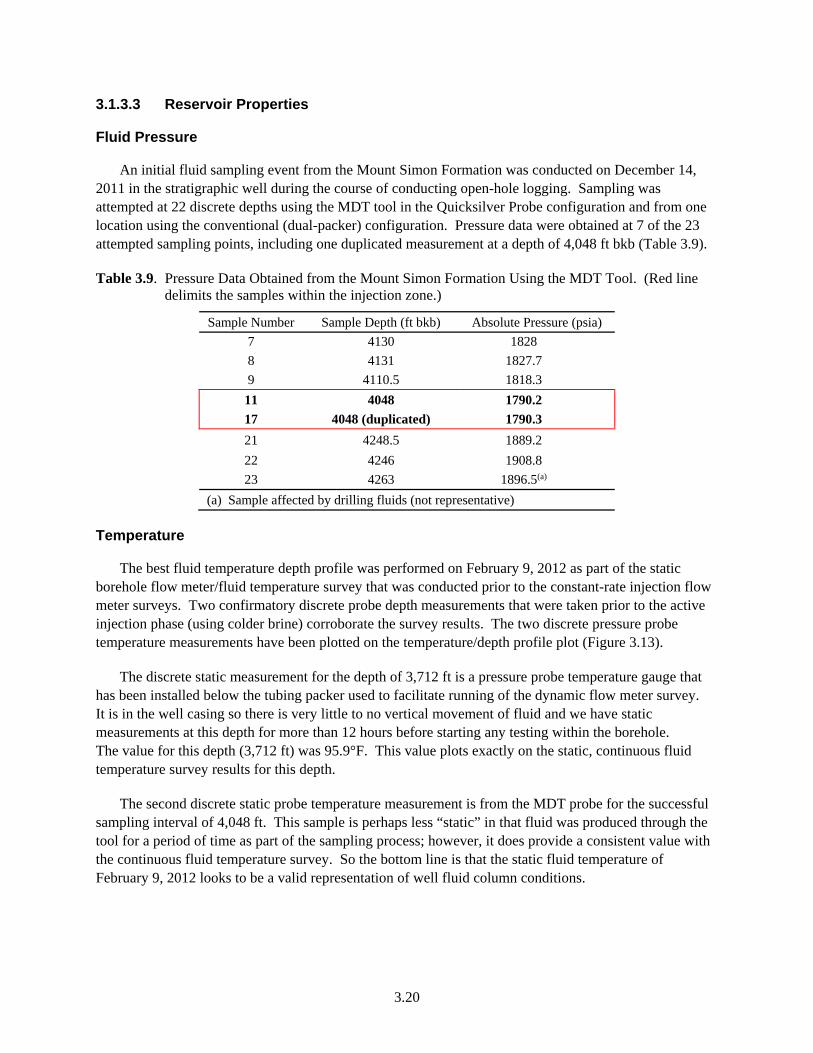
An initial fluid sampling event from the Mount Simon Formation was conducted on December 14, 2011 in the stratigraphic well during the course of conducting open-hole logging. Sampling was attempted at 22 discrete depths using the MDT tool in the Quicksilver Probe configuration and from one location using the conventional (dual-packer) configuration. Pressure data were obtained at 7 of the 23 attempted sampling points, including one duplicated measurement at a depth of 4,048 ft bkb (Table 3.9).
Table 3.9. Pressure Data Obtained from the Mount Simon Formation Using the MDT Tool. (Red line delimits the samples within the injection zone.)
Sample Number Sample Depth (ft bkb) Absolute Pressure (psia)
7 4130 1828
8 4131 1827.7
9 4110.5 1818.3
11 4048 1790.2
17 4048 (duplicated) 1790.3
21 4248.5 1889.2
22 4246 1908.8
23 4263 1896.5(a)
(a) Sample affected by drilling fluids (not representative)
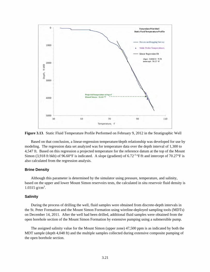
Temperature
The best fluid temperature depth profile was performed on February 9, 2012 as part of the static borehole flow meter/fluid temperature survey that was conducted prior to the constant-rate injection flow meter surveys. Two confirmatory discrete probe depth measurements that were taken prior to the active injection phase (using colder brine) corroborate the survey results. The two discrete pressure probe temperature measurements have been plotted on the temperature/depth profile plot (Figure 3.13).
The discrete static measurement for the depth of 3,712 ft is a pressure probe temperature gauge that has been installed below the tubing packer used to facilitate running of the dynamic flow meter survey. It is in the well casing so there is very little to no vertical movement of fluid and we have static measurements at this depth for more than 12 hours before starting any testing within the borehole. The value for this depth (3,712 ft) was 95.9°F. This value plots exactly on the static, continuous fluid temperature survey results for this depth.
The second discrete static probe temperature measurement is from the MDT probe for the successful sampling interval of 4,048 ft. This sample is perhaps less “static” in that fluid was produced through the tool for a period of time as part of the sampling process; however, it does provide a consistent value with the continuous fluid temperature survey. So the bottom line is that the static fluid temperature of February 9, 2012 looks to be a valid representation of well fluid column conditions.
3.21
Figure 3.13. Static Fluid Temperature Profile Performed on February 9, 2012 in the Stratigraphic Well
Based on that conclusion, a linear-regression temperature/depth relationship was developed for use by modeling. The regression data set analyzed was for temperature data over the depth interval of 1,300 to 4,547 ft. Based on this regression a projected temperature for the reference datum at the top of the Mount Simon (3,918 ft bkb) of 96.60°F is indicated. A slope (gradient) of 6.72-3 °F/ft and intercept of 70.27°F is also calculated from the regression analysis.
Brine Density
Although this parameter is determined by the simulator using pressure, temperature, and salinity, based on the upper and lower Mount Simon reservoirs tests, the calculated in situ reservoir fluid density is 1.0315 g/cm3.
Salinity
During the process of drilling the well, fluid samples were obtained from discrete-depth intervals in the St. Peter Formation and the Mount Simon Formation using wireline-deployed sampling tools (MDTs) on December 14, 2011. After the well had been drilled, additional fluid samples were obtained from the open borehole section of the Mount Simon Formation by extensive pumping using a submersible pump.
The assigned salinity value for the Mount Simon (upper zone) 47,500 ppm is as indicated by both the MDT sample (depth 4,048 ft) and the multiple samples collected during extensive composite pumping of the open borehole section.
3.22
3.1.3.4 Chemical Properties
The EPA (2011a) identified a number of chemical properties as relevant parameters for multiphase flow modeling. These include the aqueous diffusion coefficient, aqueous solubility, and solubility in CO2. The properties change significantly relative to temperature, pressure, salinity, and other variables, and are predicted by equations of state used by the model to calculate properties at conditions encountered in the simulation as they change with location and time (White et al. 2012)
3.1.3.5 Fracture Pressure in the Injection Zone
Hubbert and Willis (1957) established that the orientation of a hydraulic fracture is controlled by the orientation of the least principal stress and the pressure needed to propagate a hydraulic fracture is controlled by the magnitude of the least principal stress. Hydraulic fracturing (mini-frac, leak-off tests) is commonly used to determine the magnitude of the least principal stress (Haimson and Cornet 2003; Zoback et al. 2003). In situ determination of the fracture pressure using these methods provides the best estimation of the fracture pressure of both the injection and the confining zones. However no hydraulic fracturing test has been conducted in the stratigraphic well and no site-specific fracture pressure values are available for the confining zone and the reservoir. Other approaches (listed below) have thus been chosen to determine an appropriate value for the fracture pressure.
The geomechanical uncalibrated anisotropic elastic properties log from Schlumberger performed in the stratigraphic well could give information about the minimum horizontal stress. However, several assumptions are made and a calibration with available mini-fracs or leak-off tests is usually required to get accurate values of these elastic parameters for the studied site. These data will not be considered here.
Triaxial tests were also conducted on eight samples from the stratigraphic well (see Table 2.11 in Chapter 2.0). Samples 3 to 7 are located within the injection zone. Fracture gradients were estimated to range from 0.647 to 0.682 psi/ft, which cannot directly be compared to the fracture pressure gradient required for the permit. Triaxial tests alone cannot provide accurate measurement of fracture pressure.
Existing regional values. Similar carbon storage projects elsewhere in Illinois (in Macon and Christian counties) provide data for fracture pressure in a comparable geological context. In Macon County (CCS#1 well at Decatur), about 65 mi east of the FutureGen 2.0 proposed site, a fracture pressure gradient of 0.715 psi/ft was obtained at the base of the Mount Simon Sandstone Formation using a step-rate injection test (EPA 2011b). In Christian County, a “conservative” pressure gradient of 0.65 psi/ft was used for the same injecting zone (EPA 2011c). No site-specific data were available.
Last, the regulation relating to the “Determination of Maximum Injection Pressure for Class I Wells” in EPA Region 5 is based on the fracture closure pressure, which has been chosen to be 0.57 psi/ft for the Mount Simon Sandstone (EPA 1994).
Based on all of these considerations, a fracture pressure gradient of 0.65 psi/ft was chosen. The EPA GS Rule requires that “Except during stimulation, the owner or operator must ensure that injection pressure does not exceed 90 percent of the fracture pressure of the injection zone(s) so as to ensure that the injection does not initiate new fractures or propagate existing fractures in the injection zone(s)…” Therefore, a value of .585 psi/ft (90% of 0.65 psi/ft) was used in the model to calculate the maximum injection pressure.
3.23
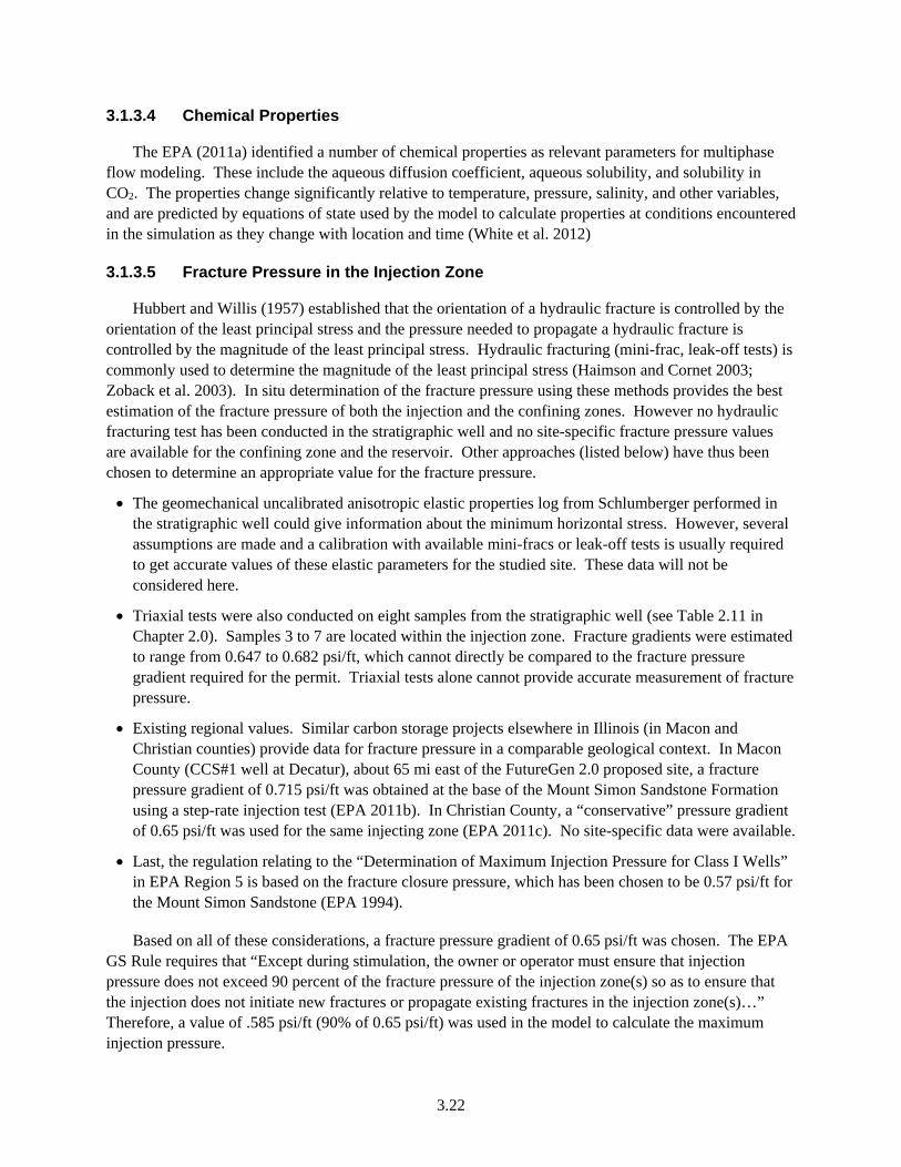
3.1.4 Numerical Model Implementation
As described above, the model domain for the Morgan County CO2 storage site consists of the injection zone (Mount Simon and Elmhurst), the primary confining zone (Lombard and Proviso), the Ironton-Galesville, and the secondary confining zone (Davis-Ironton and the Franconia). Preliminary simulations were conducted to determine the extent of the model domain so that lateral boundaries were distant enough from the injection location so as not to influence the model results. The three-dimensional, boundary-fitted numerical model grid was designed to have constant grid spacing with higher resolution in the area influenced by the CO2 injection (3- by 3-mi area), with increasingly larger grid spacing moving out in all lateral directions toward the domain boundary.
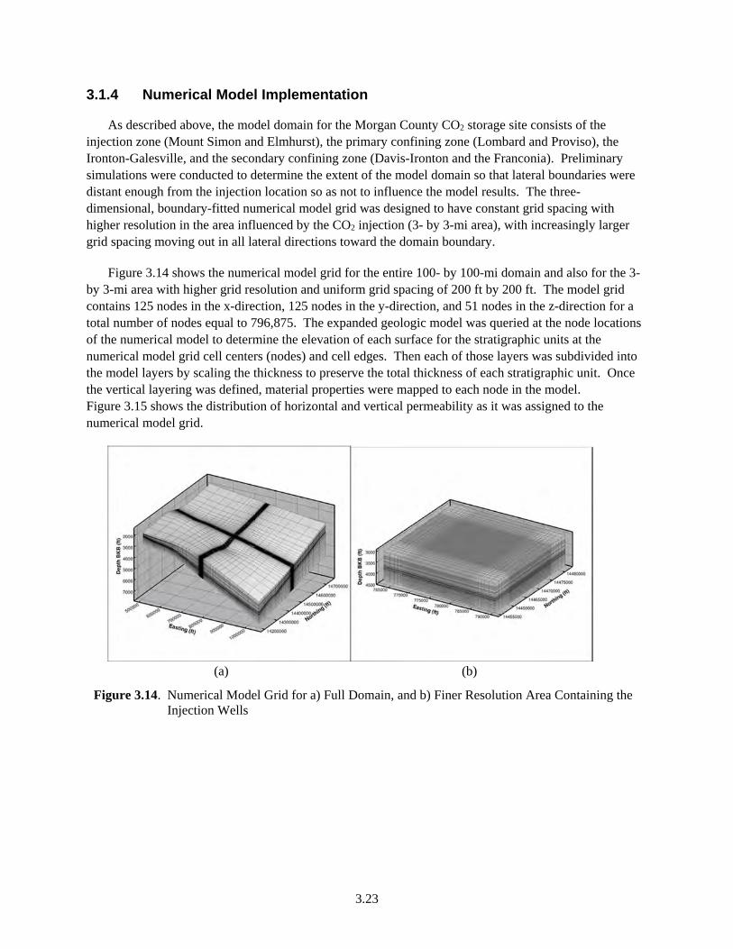
Figure 3.14 shows the numerical model grid for the entire 100- by 100-mi domain and also for the 3- by 3-mi area with higher grid resolution and uniform grid spacing of 200 ft by 200 ft. The model grid contains 125 nodes in the x-direction, 125 nodes in the y-direction, and 51 nodes in the z-direction for a total number of nodes equal to 796,875. The expanded geologic model was queried at the node locations of the numerical model to determine the elevation of each surface for the stratigraphic units at the numerical model grid cell centers (nodes) and cell edges. Then each of those layers was subdivided into the model layers by scaling the thickness to preserve the total thickness of each stratigraphic unit. Once the vertical layering was defined, material properties were mapped to each node in the model. Figure 3.15 shows the distribution of horizontal and vertical permeability as it was assigned to the numerical model grid.
(a) (b)
Figure 3.14. Numerical Model Grid for a) Full Domain, and b) Finer Resolution Area Containing the Injection Wells
3.24
(a) (b)
Figure 3.15. Permeability Assigned to Numerical Model a) Horizontal Permeability; b) Vertical Permeability
3.1.4.1 Initial Conditions
The reservoir is assumed to be under hydrostatic conditions with no regional or local flow conditions. Therefore the hydrologic flow system is assumed to be at steady state until the start of injection. To achieve this with the STOMP-CO2 simulator one can either run an initial simulation (executed for a very long time period until steady-state conditions are achieved) to generate the initial distribution of pressure, temperature, and salinity conditions in the model from an initial guess, or one can specify the initial conditions at a reference depth using the hydrostatic option, allowing the simulator to calculate and assign the initial conditions to all the model nodes. Site-specific data were available for pressure, temperature, and salinity, and therefore the hydrostatic option was used to assign initial conditions. A temperature gradient was specified based on the geothermal gradient, but the initial salinity was considered to be constant for the entire domain. A summary of the initial conditions is presented in Table 3.10.
Table 3.10. Summary of Initial Conditions
Parameter Reference
Depth (bkb) Value
Reservoir Pressure 4,048 ft 1,790.2 psi Aqueous Saturation 1.0 Reservoir Temperature 3,918 ft 96.6 °F Temperature Gradient 0.00672 °F/ft Salinity 47,500 ppm
3.1.4.2 Boundary Conditions
Boundary conditions were established with the assumption that the reservoir is continuous throughout the region and that the underlying Precambrian unit is impermeable. Therefore, the bottom boundary was set as a no-flow boundary for aqueous fluids and for the CO2-rich phase. The lateral and top boundary conditions were set to hydrostatic pressure using the initial condition with the assumption that each of these boundaries is distant enough from the injection zone to have minimal to no effect on the CO2 plume migration and pressure distribution.
3.25
3.1.4.3 Simulation Time Period
The EPA GS Rule requires that owners or operators must “Predict, using existing site characterization, monitoring and operational data, and computational modeling, the projected lateral and vertical migration of the CO2 plume and formation fluids in the subsurface from the commencement of injection activities until the plume movement ceases, until pressure differentials sufficient to cause the movement of injected fluids or formation fluids into a USDW are no longer present, or until the end of a fixed time period as determined by the Director.” Simulations were conducted to determine the total simulation time needed to satisfy the required conditions, and those results are presented in this section.
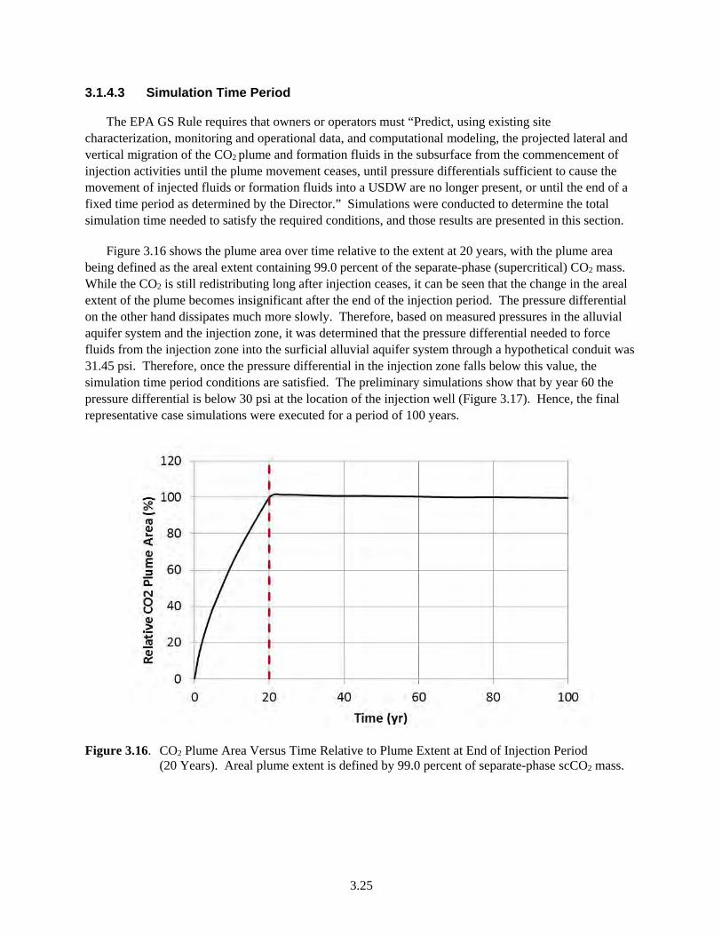
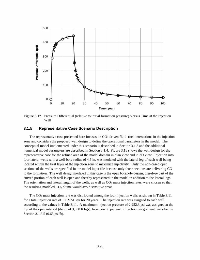
Figure 3.16 shows the plume area over time relative to the extent at 20 years, with the plume area being defined as the areal extent containing 99.0 percent of the separate-phase (supercritical) CO2 mass. While the CO2 is still redistributing long after injection ceases, it can be seen that the change in the areal extent of the plume becomes insignificant after the end of the injection period. The pressure differential on the other hand dissipates much more slowly. Therefore, based on measured pressures in the alluvial aquifer system and the injection zone, it was determined that the pressure differential needed to force fluids from the injection zone into the surficial alluvial aquifer system through a hypothetical conduit was 31.45 psi. Therefore, once the pressure differential in the injection zone falls below this value, the simulation time period conditions are satisfied. The preliminary simulations show that by year 60 the pressure differential is below 30 psi at the location of the injection well (Figure 3.17). Hence, the final representative case simulations were executed for a period of 100 years.
Figure 3.16. CO2 Plume Area Versus Time Relative to Plume Extent at End of Injection Period (20 Years). Areal plume extent is defined by 99.0 percent of separate-phase scCO2 mass.
3.26
Figure 3.17. Pressure Differential (relative to initial formation pressure) Versus Time at the Injection Well
3.1.5 Representative Case Scenario Description
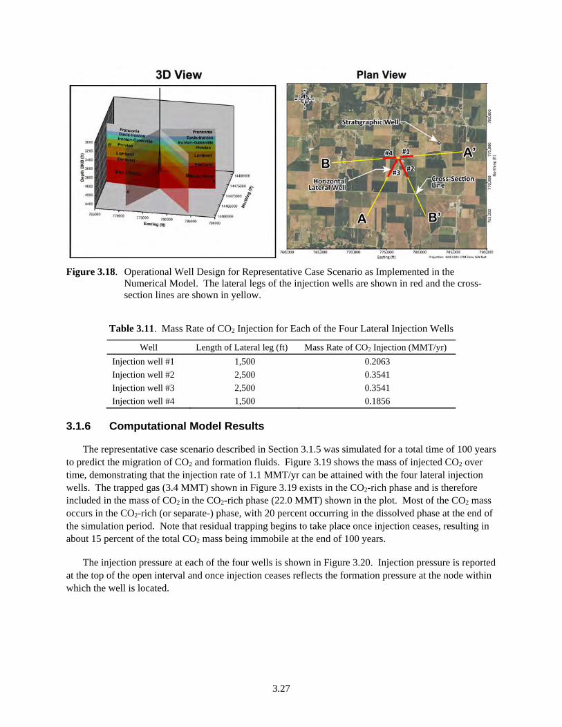
The representative case presented here focuses on CO2-driven fluid–rock interactions in the injection zone and considers the proposed well design to define the operational parameters in the model. The conceptual model implemented under this scenario is described in Section 3.1.3 and the additional numerical model parameters are described in Section 3.1.4. Figure 3.18 shows the well design for the representative case for the refined area of the model domain in plan view and in 3D view. Injection into four lateral wells with a well-bore radius of 4.5 in. was modeled with the lateral leg of each well being located within the best layer of the injection zone to maximize injectivity. Only the non-cased open sections of the wells are specified in the model input file because only those sections are delivering CO2 to the formation. The well design modeled in this case is the open borehole design, therefore part of the curved portion of each well is open and thereby represented in the model in addition to the lateral legs. The orientation and lateral length of the wells, as well as CO2 mass injection rates, were chosen so that the resulting modeled CO2 plume would avoid sensitive areas.
The CO2 mass injection rate was distributed among the four injection wells as shown in Table 3.11 for a total injection rate of 1.1 MMT/yr for 20 years. The injection rate was assigned to each well according to the values in Table 3.11. A maximum injection pressure of 2,252.3 psi was assigned at the top of the open interval (depth of 3,850 ft bgs), based on 90 percent of the fracture gradient described in Section 3.1.3.5 (0.65 psi/ft).
3.27
Figure 3.18. Operational Well Design for Representative Case Scenario as Implemented in the Numerical Model. The lateral legs of the injection wells are shown in red and the cross-section lines are shown in yellow.
Table 3.11. Mass Rate of CO2 Injection for Each of the Four Lateral Injection Wells
Well Length of Lateral leg (ft) Mass Rate of CO2 Injection (MMT/yr)
Injection well #1 1,500 0.2063
Injection well #2 2,500 0.3541
Injection well #3 2,500 0.3541
Injection well #4 1,500 0.1856
3.1.6 Computational Model Results
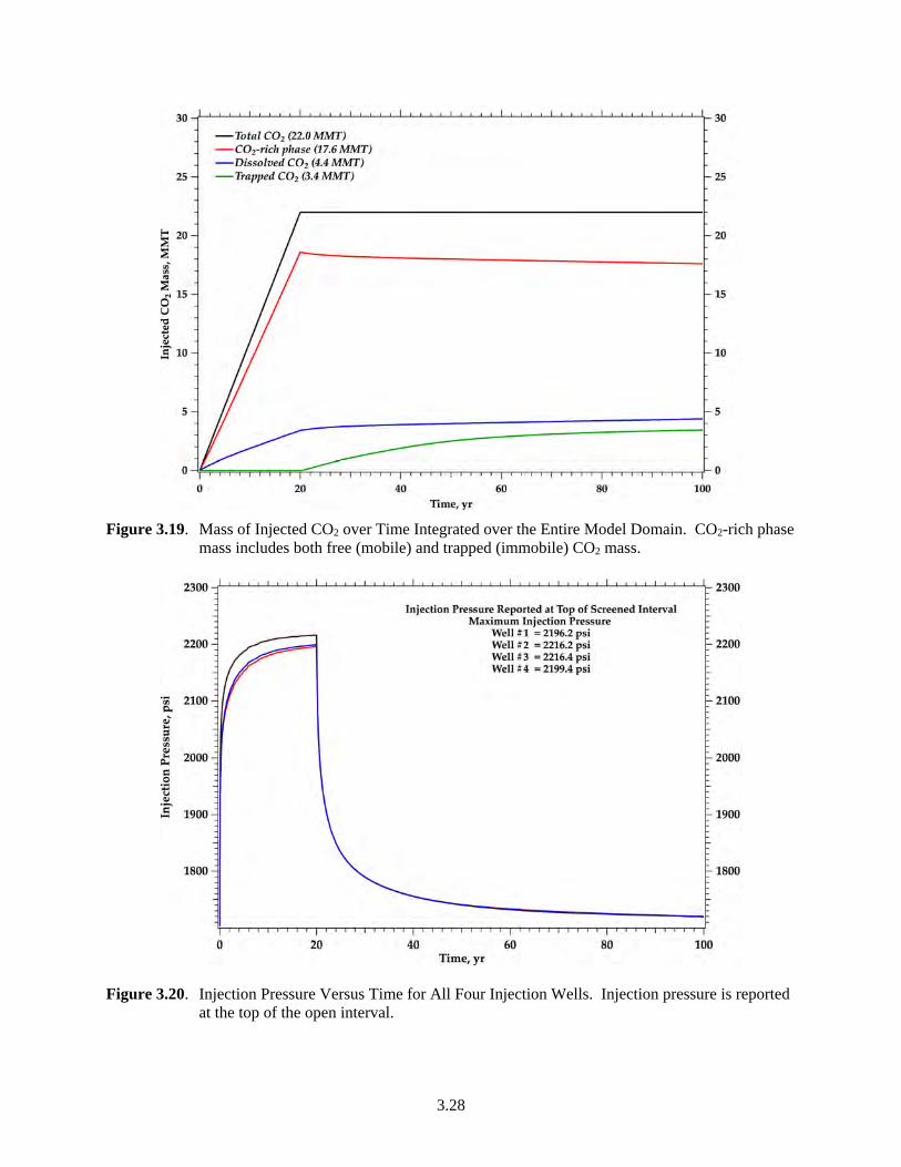
The representative case scenario described in Section 3.1.5 was simulated for a total time of 100 years to predict the migration of CO2 and formation fluids. Figure 3.19 shows the mass of injected CO2 over time, demonstrating that the injection rate of 1.1 MMT/yr can be attained with the four lateral injection wells. The trapped gas (3.4 MMT) shown in Figure 3.19 exists in the CO2-rich phase and is therefore included in the mass of CO2 in the CO2-rich phase (22.0 MMT) shown in the plot. Most of the CO2 mass occurs in the CO2-rich (or separate-) phase, with 20 percent occurring in the dissolved phase at the end of the simulation period. Note that residual trapping begins to take place once injection ceases, resulting in about 15 percent of the total CO2 mass being immobile at the end of 100 years.
The injection pressure at each of the four wells is shown in Figure 3.20. Injection pressure is reported at the top of the open interval and once injection ceases reflects the formation pressure at the node within which the well is located.
3.28
Figure 3.19. Mass of Injected CO2 over Time Integrated over the Entire Model Domain. CO2-rich phase mass includes both free (mobile) and trapped (immobile) CO2 mass.
Figure 3.20. Injection Pressure Versus Time for All Four Injection Wells. Injection pressure is reported at the top of the open interval.

3.29
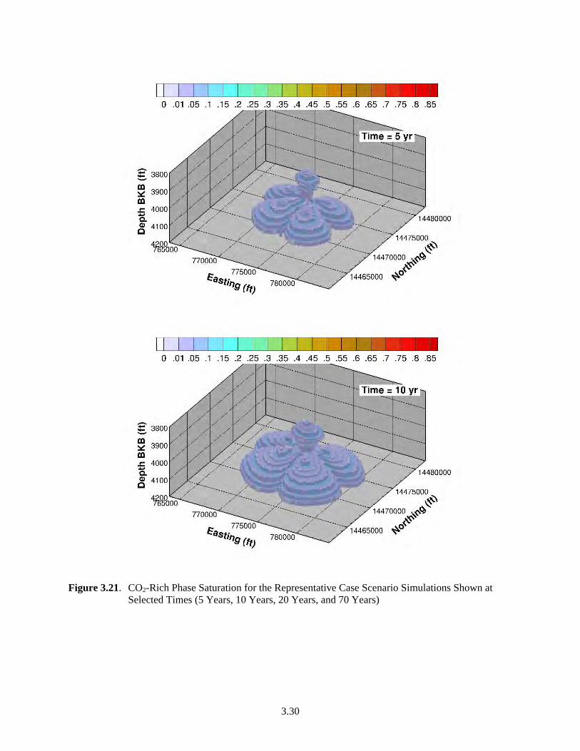
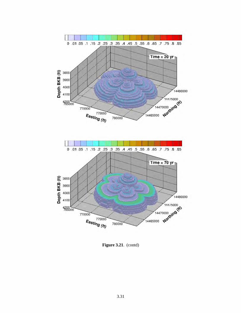
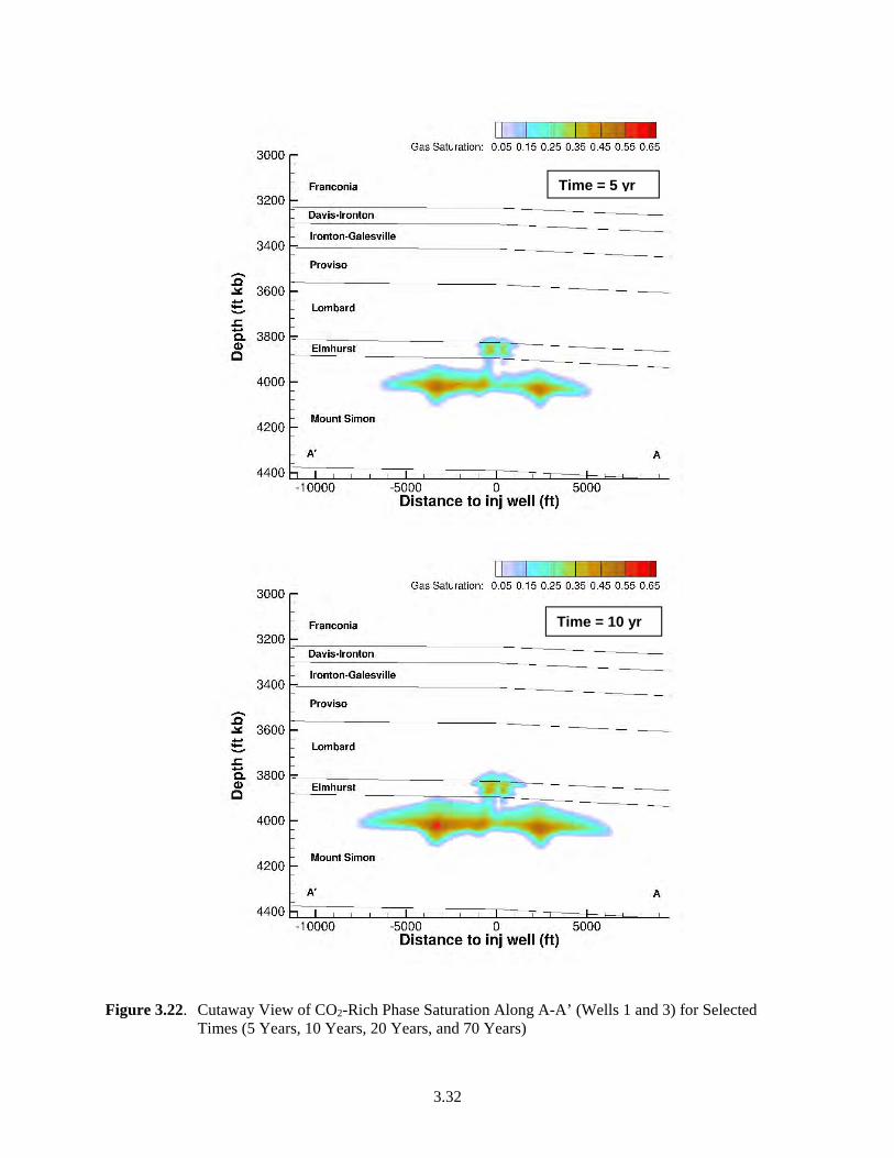
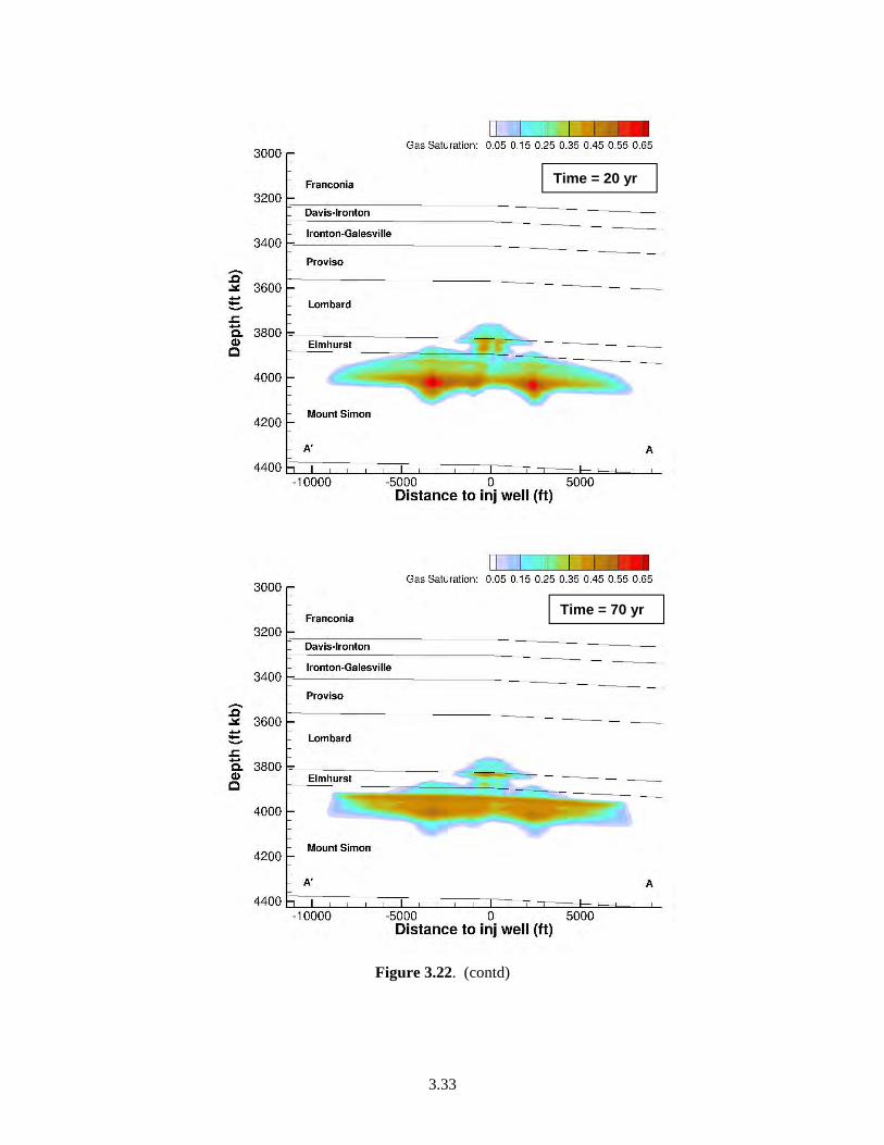
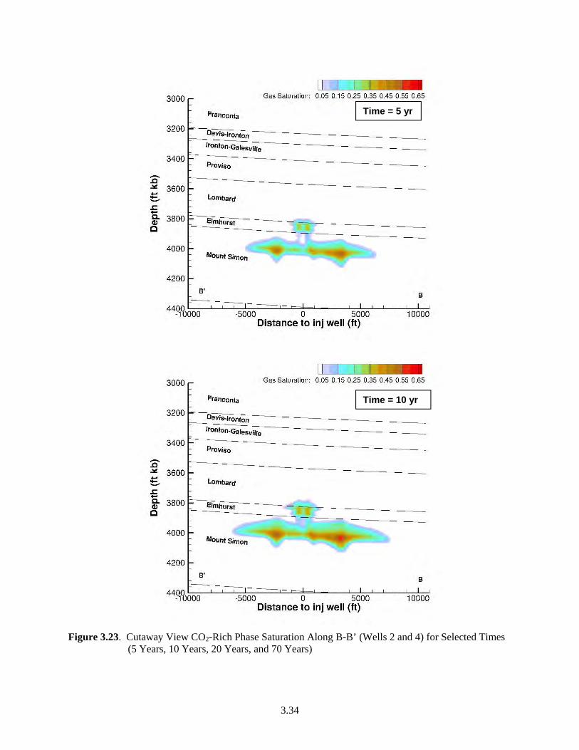
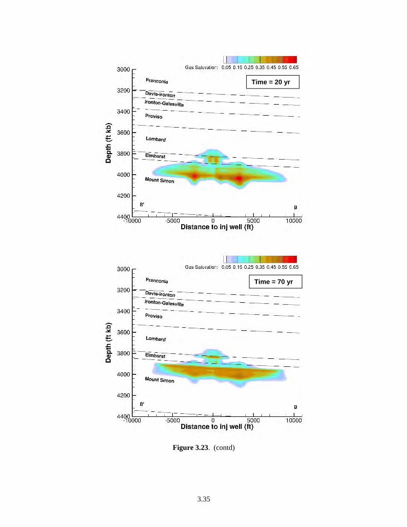
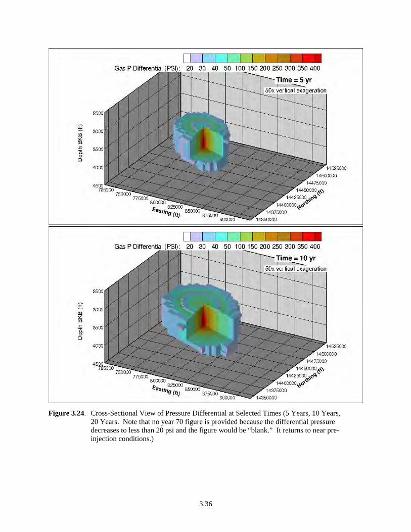
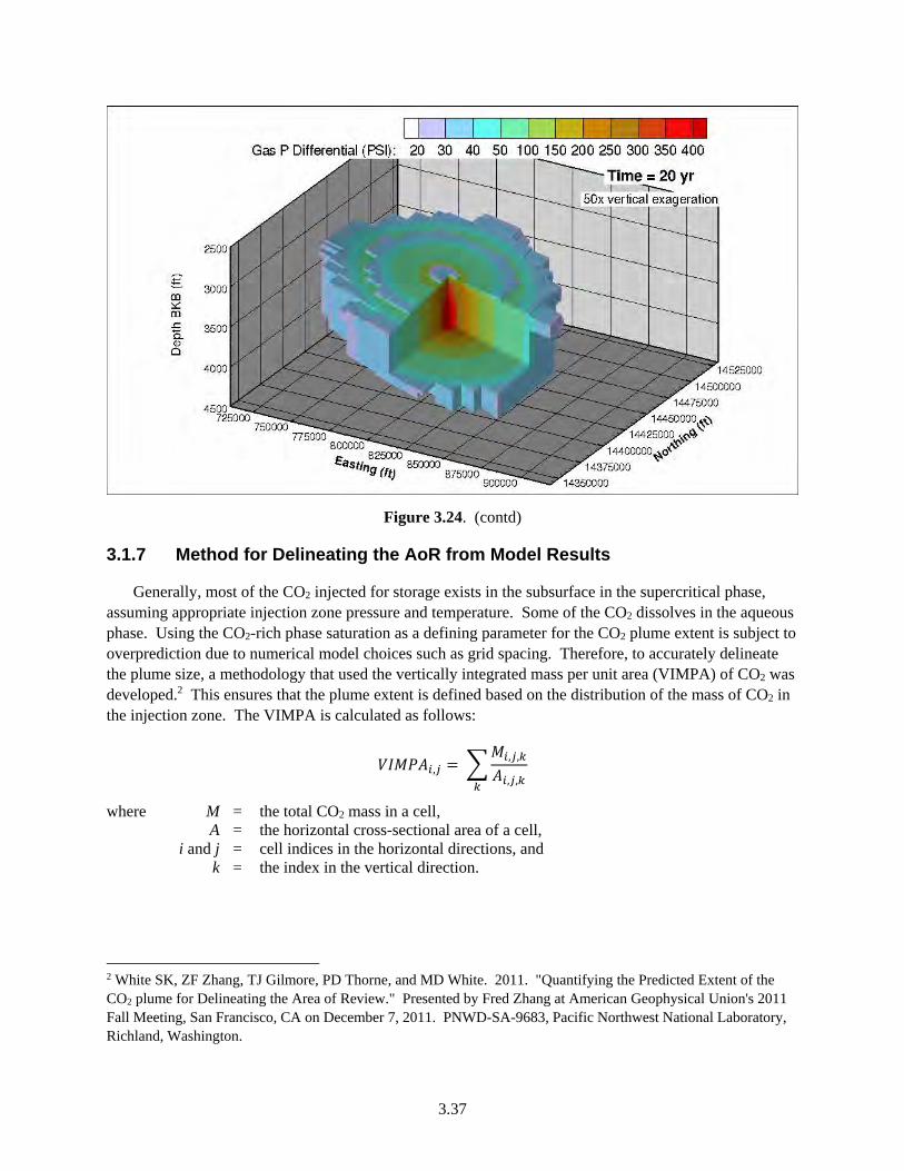
Reservoir conditions are such that the CO2 remains in the supercritical state throughout the domain and for the entire simulation period. The CO2-rich (or separate-) phase saturation is presented for selected time planes in Figure 3.21. The CO2 plume forms a cloverleaf pattern as a result of the four lateral-injection-well design. A cross-sectional view of the CO2 plume is presented as slices through the well centers and along the well trace (see Figure 3.18 for location of cross sections). Figure 3.22 and Figure 3.23 show the CO2-rich (or separate) phase saturation for selected times for slices A-A’ and B-B’, respectively. The pressure differential across the model domain for selected times is shown in Figure 3.24. The pressure differential at 70 years is not shown because the maximum pressure differential at that time is below 30 psi. The plume grows both laterally and vertically as injection continues. Most of the CO2 resides in the Mount Simon Sandstone. A small amount of CO2 enters into the Elmhurst and the lower part of the primary confining zone (Lombard). When injection ceases at 20 years, the lateral growth becomes negligible but the plume continues to move slowly primarily upward. Once CO2 reaches the low-permeability zone in the upper Mount Simon it begins to move laterally. There is no additional CO2 entering the confining zone from the injection zone after injection ceases.
3.30
Figure 3.21. CO2-Rich Phase Saturation for the Representative Case Scenario Simulations Shown at Selected Times (5 Years, 10 Years, 20 Years, and 70 Years)
3.31
Figure 3.21. (contd)
3.32
Figure 3.22. Cutaway View of CO2-Rich Phase Saturation Along A-A’ (Wells 1 and 3) for Selected Times (5 Years, 10 Years, 20 Years, and 70 Years)
Time = 5 yr
Time = 10 yr
3.33
Figure 3.22. (contd)
Time = 20 yr
Time = 70 yr
3.34
Figure 3.23. Cutaway View CO2-Rich Phase Saturation Along B-B’ (Wells 2 and 4) for Selected Times (5 Years, 10 Years, 20 Years, and 70 Years)
Time = 5 yr
Time = 10 yr
3.35
Figure 3.23. (contd)
Time = 20 yr
Time = 70 yr
3.36
Figure 3.24. Cross-Sectional View of Pressure Differential at Selected Times (5 Years, 10 Years, 20 Years. Note that no year 70 figure is provided because the differential pressure decreases to less than 20 psi and the figure would be “blank.” It returns to near pre-injection conditions.)
3.37
Figure 3.24. (contd)
3.1.7 Method for Delineating the AoR from Model Results
Generally, most of the CO2 injected for storage exists in the subsurface in the supercritical phase, assuming appropriate injection zone pressure and temperature. Some of the CO2 dissolves in the aqueous phase. Using the CO2-rich phase saturation as a defining parameter for the CO2 plume extent is subject to overprediction due to numerical model choices such as grid spacing. Therefore, to accurately delineate the plume size, a methodology that used the vertically integrated mass per unit area (VIMPA) of CO2 was developed.2 This ensures that the plume extent is defined based on the distribution of the mass of CO2 in the injection zone. The VIMPA is calculated as follows:
, , ,
, ,
where M = the total CO2 mass in a cell, A = the horizontal cross-sectional area of a cell, i and j = cell indices in the horizontal directions, and k = the index in the vertical direction.
2 White SK, ZF Zhang, TJ Gilmore, PD Thorne, and MD White. 2011. "Quantifying the Predicted Extent of the CO2 plume for Delineating the Area of Review." Presented by Fred Zhang at American Geophysical Union's 2011 Fall Meeting, San Francisco, CA on December 7, 2011. PNWD-SA-9683, Pacific Northwest National Laboratory, Richland, Washington.
3.38
The VIMPA may be calculated for the CO2-rich phase or the dissolved CO2, or the total CO2 for the entire vertical depth or for a specific layer or layers (e.g., the injection zone). The VIMPA distributes non-uniformly in the horizontal plane. Generally, the VIMPA is larger near the injection well and decreases gradually away from the well. For certain geologic conditions, the plume size defined by the area that contains all of the CO2 mass can be very large, while in fact, most of the mass may reside in a subregion of that area. For the purposes of AoR determination, the extent of the plume is defined as the contour line of VIMPA, within which 99.0 percent of the CO2-rich phase (separate-phase) mass is contained. The acreage (areal extent in acres) of the plume is calculated by integrating all cells within the plume extent. Therefore, the CO2 plume referred to in this document is defined as the area containing 99.0 percent of the separate phase CO2 mass.
3.1.8 Delineation of the AoR
The AoR for the Morgan County site is based on the predicted areal extent encompassing 99.0 percent of the separate phase CO2 mass after 20 years of injection and 2 years of shut-in (being temporarily sealed) (see Section 3.1). A larger, 25-mi2 area that represents an expanded search area used to identify the existence of any confining zone penetrations (see Section 3.2.1) is also identified. As described in Section 3.1, the site conditions result in an infinite AoR when using the EPA-suggested methodology for calculating a pressure front based on the lowermost USDW. Planned control measures will be implemented by the Monitoring, Verification, and Accounting Program to ensure that the FutureGen 2.0 Project is protective of USDWs and in addition natural geologic features will help mitigate impacts on USDWs in the event that an unforeseen injection zone containment loss were to occur. These control measures and natural geologic features that protect the USDW include the following:
planned early detection monitoring within the interval immediately above the primary confining zone (Ironton Sandstone)
planned development of an environmental release model, which will encompass the overburden materials between the injection zone and ground surface and will be used to predict vertical CO2 and/or brine migration under various containment-loss scenarios, and to assess the potential for impacts on shallow USDWs.
the disparity in the calculated hydraulic head measurements (together with the significant formation fluid salinity differences), which suggests that groundwaters within the St. Peter and Mount Simon bedrock aquifers are naturally and physically isolated from one another, providing indication that there are no significant conduits (open well bores or fracturing) between these two formations and that the Eau Claire forms an effective confining layer
the presence of secondary confining zones and the relatively high-permeability Potosi dolomite interval, which would both act to limit vertical migration to USDWs if primary containment were lost
After 20 years of injection and 2 years of shut-in, the areal extent of the separate-phase CO2 plume no longer increases significantly. Therefore, the AoR, shown in Figure 3.25, is delineated based on the predicted areal extent of the separate-phase CO2 plume at 22 years.
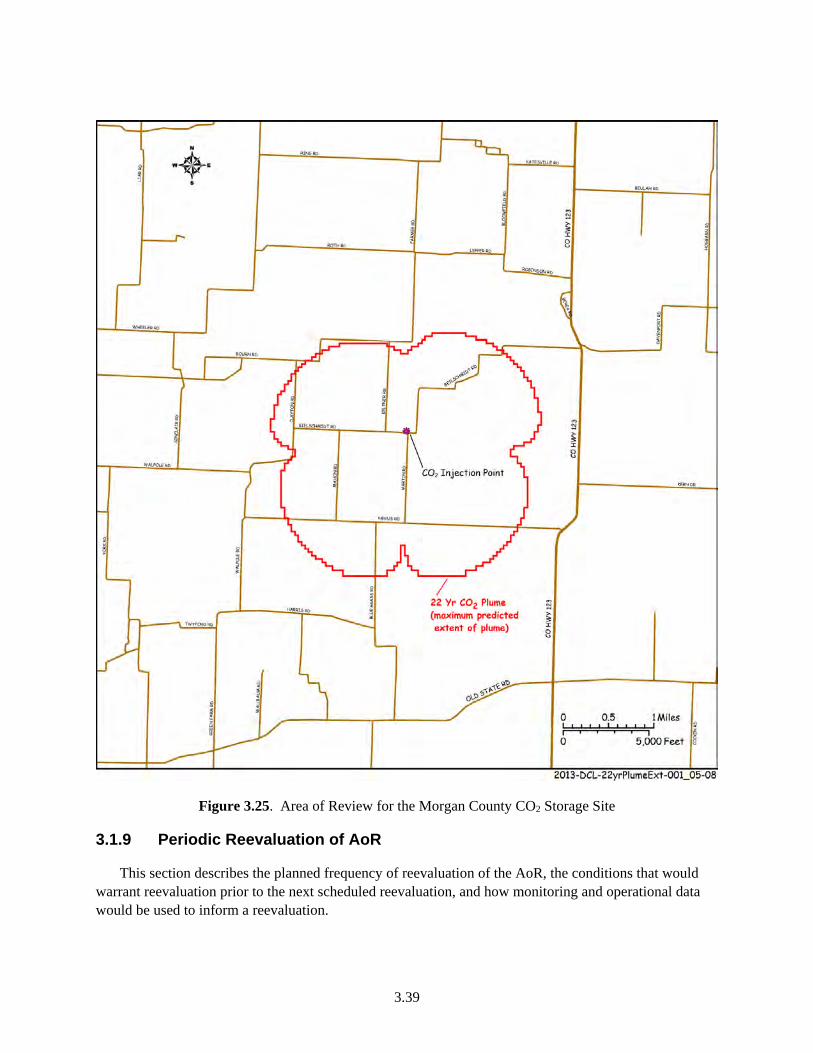
3.39
Figure 3.25. Area of Review for the Morgan County CO2 Storage Site
3.1.9 Periodic Reevaluation of AoR
This section describes the planned frequency of reevaluation of the AoR, the conditions that would warrant reevaluation prior to the next scheduled reevaluation, and how monitoring and operational data would be used to inform a reevaluation.

3.40
3.1.9.1 Minimum Frequency
The Alliance will reevaluate the AoR, at a minimum, every 5 years after issuance of a UIC Class VI permit and initiation of injection operations, as required by 40 CFR 146.84(b)(2)(i). The reevaluation will be based on site-specific information as described in the following sections. Although the Alliance will reevaluate the AoR every 5 years, some conditions would warrant reevaluation prior to the next scheduled reevaluation. These conditions include 1) a significant change in operations such as a prolonged increase or decrease in the CO2 injection rates at the injections wells, 2) a significant difference between simulated and observed pressure and CO2 arrival response at site monitoring wells, or 3) newly collected characterization data that have a significant effect on the site computational model. If any of these conditions occurs, the Alliance will reevaluate the AoR as described below.
3.1.9.2 Operational and Monitoring Data and Model Calibration
As discussed in the Chapter 5.0 (Testing and Monitoring Plan), the monitoring program will adopt 1) both direct and indirect monitoring methodologies for assessing CO2 fate and transport within the injection zone, 2) direct monitoring of the lowermost USDW, and 3) other near-surface-monitoring technologies (as needed to meet project or regulatory requirements), including soil-gas, atmospheric, and ecological monitoring.
Ongoing direct and indirect monitoring data, which provide relevant information for understanding the development and evolution of the CO2 plume, will be used to support reevaluation of the AoR. These data include 1) the chemical and physical characteristics of the CO2 injection stream based on sampling and analysis; 2) continuous monitoring of injection mass flow rate, pressure, temperature, and fluid volume; 3) measurements of pressure response at all site monitoring wells; and 4) CO2 arrival and transport response at all site monitoring wells based on direct aqueous measurements and selected indirect monitoring method(s). The Alliance will compare these observational data with predicted responses from the computational model and if significant discrepancies between the observed and predicted responses exist, the monitoring data will be used to recalibrate the model (Figure 3.26). In cases where the observed monitoring data agree with model predictions, an AoR reevaluation will consist of a demonstration that monitoring data are consistent with modeled predictions.
As additional characterization data are collected, the site conceptual model will be revised and the modeling steps described above will be repeated to incorporate new knowledge about the site.
3.1.9.3 Report of the AoR Reevaluation
The Alliance will submit a report notifying the UIC Program Director of the results of this reevaluation. At that time, the Alliance will either 1) submit the monitoring data and modeling results to demonstrate that no adjustment to the AoR is required, or 2) modify its Corrective Action, Emergency and Remedial Response and other plans to account for the revised AoR. All modeling inputs and data used to support AoR reevaluations will be retained by the Alliance for 10 years.
To the extent that the reevaluated AoR is different from the one identified in this supporting documentation, the Alliance will identify all active and abandoned wells and underground mines that penetrate the confining zone (the Eau Claire Formation) in the reevaluated AoR and will perform corrective actions on those wells in the manner described in Section 3.2.2. As needed, the Alliance will revise all other plans, such as the Emergency and Remedial Response Plan, to take into account the reevaluated AoR and will submit those plans to the UIC Program Director for review and approval.
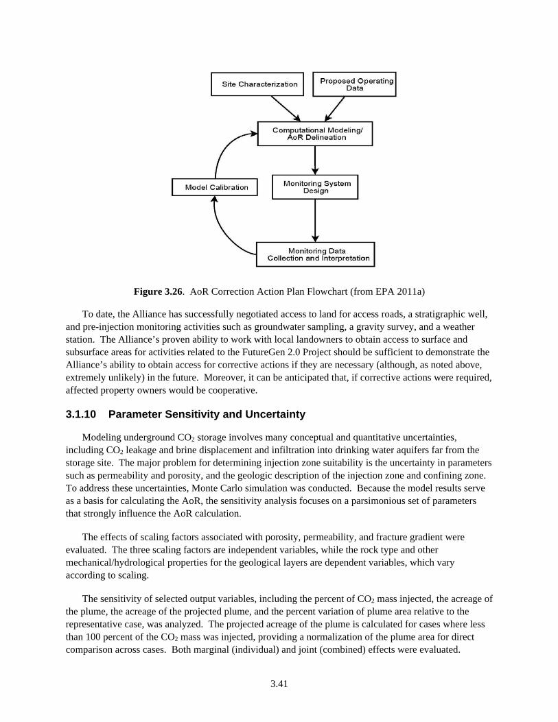
3.41
Figure 3.26. AoR Correction Action Plan Flowchart (from EPA 2011a)
To date, the Alliance has successfully negotiated access to land for access roads, a stratigraphic well, and pre-injection monitoring activities such as groundwater sampling, a gravity survey, and a weather station. The Alliance’s proven ability to work with local landowners to obtain access to surface and subsurface areas for activities related to the FutureGen 2.0 Project should be sufficient to demonstrate the Alliance’s ability to obtain access for corrective actions if they are necessary (although, as noted above, extremely unlikely) in the future. Moreover, it can be anticipated that, if corrective actions were required, affected property owners would be cooperative.
3.1.10 Parameter Sensitivity and Uncertainty
Modeling underground CO2 storage involves many conceptual and quantitative uncertainties, including CO2 leakage and brine displacement and infiltration into drinking water aquifers far from the storage site. The major problem for determining injection zone suitability is the uncertainty in parameters such as permeability and porosity, and the geologic description of the injection zone and confining zone. To address these uncertainties, Monte Carlo simulation was conducted. Because the model results serve as a basis for calculating the AoR, the sensitivity analysis focuses on a parsimonious set of parameters that strongly influence the AoR calculation.
The effects of scaling factors associated with porosity, permeability, and fracture gradient were evaluated. The three scaling factors are independent variables, while the rock type and other mechanical/hydrological properties for the geological layers are dependent variables, which vary according to scaling.
The sensitivity of selected output variables, including the percent of CO2 mass injected, the acreage of the plume, the acreage of the projected plume, and the percent variation of plume area relative to the representative case, was analyzed. The projected acreage of the plume is calculated for cases where less than 100 percent of the CO2 mass was injected, providing a normalization of the plume area for direct comparison across cases. Both marginal (individual) and joint (combined) effects were evaluated.
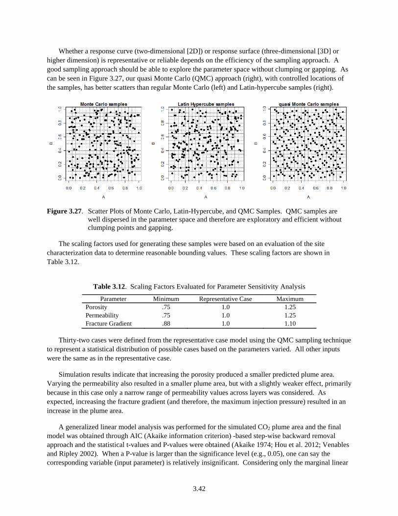
3.42
Whether a response curve (two-dimensional [2D]) or response surface (three-dimensional [3D] or higher dimension) is representative or reliable depends on the efficiency of the sampling approach. A good sampling approach should be able to explore the parameter space without clumping or gapping. As can be seen in Figure 3.27, our quasi Monte Carlo (QMC) approach (right), with controlled locations of the samples, has better scatters than regular Monte Carlo (left) and Latin-hypercube samples (right).
Figure 3.27. Scatter Plots of Monte Carlo, Latin-Hypercube, and QMC Samples. QMC samples are well dispersed in the parameter space and therefore are exploratory and efficient without clumping points and gapping.
The scaling factors used for generating these samples were based on an evaluation of the site characterization data to determine reasonable bounding values. These scaling factors are shown in Table 3.12.
Table 3.12. Scaling Factors Evaluated for Parameter Sensitivity Analysis
Parameter Minimum Representative Case Maximum Porosity .75 1.0 1.25 Permeability .75 1.0 1.25 Fracture Gradient .88 1.0 1.10
Thirty-two cases were defined from the representative case model using the QMC sampling technique to represent a statistical distribution of possible cases based on the parameters varied. All other inputs were the same as in the representative case.
Simulation results indicate that increasing the porosity produced a smaller predicted plume area. Varying the permeability also resulted in a smaller plume area, but with a slightly weaker effect, primarily because in this case only a narrow range of permeability values across layers was considered. As expected, increasing the fracture gradient (and therefore, the maximum injection pressure) resulted in an increase in the plume area.
A generalized linear model analysis was performed for the simulated CO2 plume area and the final model was obtained through AIC (Akaike information criterion) -based step-wise backward removal approach and the statistical t-values and P-values were obtained (Akaike 1974; Hou et al. 2012; Venables and Ripley 2002). When a P-value is larger than the significance level (e.g., 0.05), one can say the corresponding variable (input parameter) is relatively insignificant. Considering only the marginal linear
3.43
effects, the fracture gradient and porosity are the most significant parameters for determining plume size. However, when the interactions are included, the combination of permeability and fracture gradient becomes significant.
The injectivity varied from the representative base case by about 50 percent for cases either with low permeability, low fracture gradient, or a combination of both. Because the injection rate was specified as a maximum rate, it was not possible to determine if, in some cases, more than 100 percent of the mass could be injected and if so, how much more. The predicted plume area varied from the representative case by about 80 to 120 percent, which is approximately the same as the variation in permeability and porosity.
3.2 Corrective Action Plan
With the AoR identified using computational modeling, EPA Class VI regulations require the identification of all confining zone penetrations within the AoR that may become a preferential pathway for leakage of CO2 and/or formation brine fluids out of the injection zone, and if necessary, performance of corrective actions to prevent leakage that could potentially cause endangerment to a USDW. The following sections discuss the findings of an evaluation that was performed to 1) identify existing penetrations within a 25-mi2 region that extends beyond the AoR (see Figure 3.28); 2) determine if any penetrations extend below the primary confining zone, thereby presenting a risk of leakage that may require corrective actions; and 3) identify corrective actions and define the approach that will be taken to prevent leakage that could endanger a USDW.
3.2.1 Identification of Primary Confining Zone Penetrations
The potential for the presence of natural primary confining zone penetrations (i.e., faults and fracture zones) was evaluated by reviewing existing maps and publications to identify any available information about local geologic structures, faults, and seismicity. Additional site-specific information was obtained from 2D seismic lines acquired within the project AoR and from preliminary borehole geophysical log data acquired from the FutureGen 2.0 stratigraphic well. Artificial penetrations (i.e., wells) were initially identified using data available online from the ISGS interactive map tools (ISGS 2012a, 2011), followed by a detailed review of historical well log records obtained from the ISGS Geologic Records Unit (ISGS 2012b).
Based on the information evaluated during this review and with the exception of the stratigraphic well, no natural or artificial penetrations have been identified within the AoR that penetrate the primary confining zone or the injection zone. The closest wells identified that penetrate the primary confining zone are approximately 16 mi south-southwest of the proposed Morgan County storage site (Figure 3.28). Although these wells are well outside the AoR, they are within the region where increased pressures in the injection zone are expected and were therefore considered for additional review. The well records obtained during this review suggest that all primary confining zone penetrations found have been properly constructed, plugged, and/or are currently in use, and do not present a risk for direct leakage and migration of fluids out of the injection zone, and will therefore not be considered for corrective action.
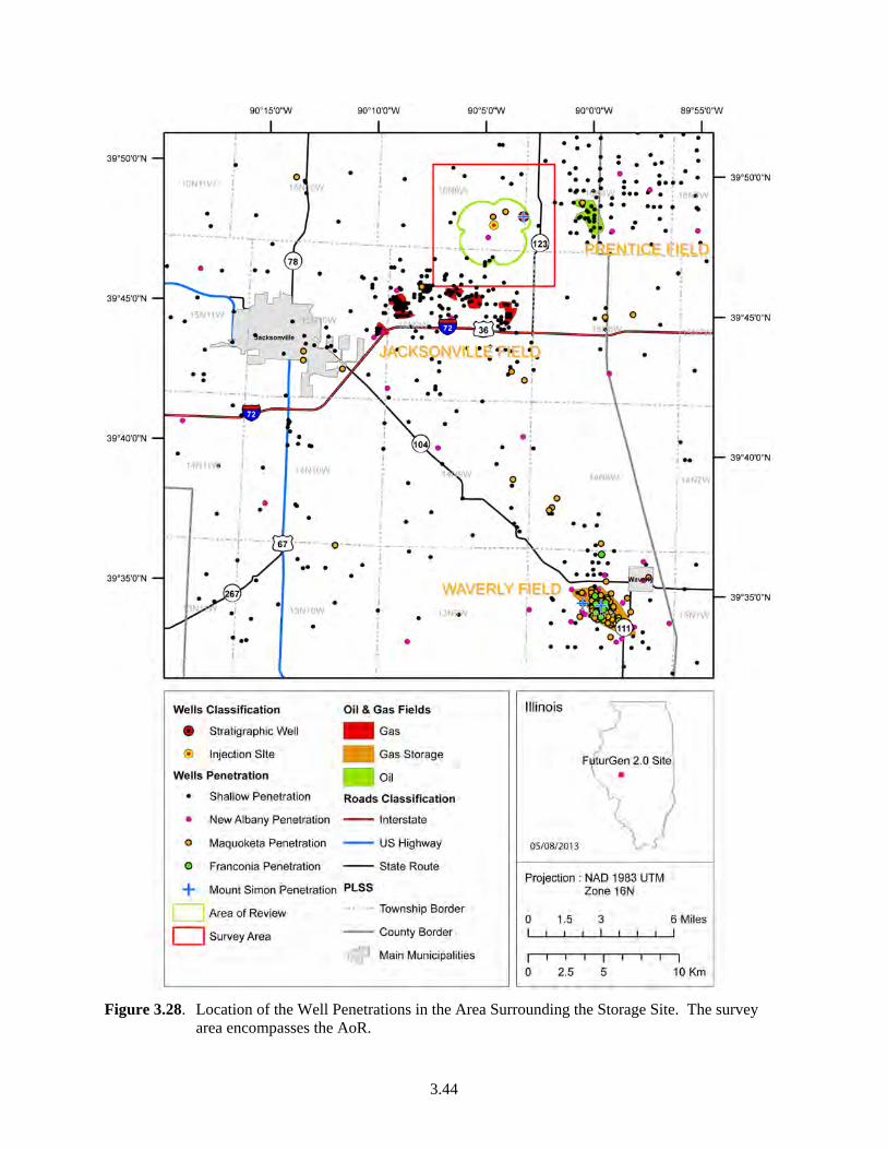
3.44
Figure 3.28. Location of the Well Penetrations in the Area Surrounding the Storage Site. The survey area encompasses the AoR.
3.45
A more detailed discussion of the geologic features of the confining zones and local geologic structures, faulting, seismicity, and available geomechanical information is presented in Chapter 2.0.
With the exception of the stratigraphic well, the nearest wells that have penetrated through the primary confining zone (Eau Claire Formation) and into the injection zone (Mount Simon Sandstone) are more than 16 mi away in the Waverly Storage Field (Figure 3.28), south-southwest of the proposed storage site, and are not in the AoR. The two boreholes, the Criswell #1-16 (API number 121370034900) and Whitlock #7-15 (API number 121370034601), are part of the Waverly Storage Field, which is an active natural-gas storage facility that is currently operated by Panhandle Eastern Pipeline Company. The primary storage reservoir used at the Waverly Storage Field is the St. Peter Sandstone. However, several wells were drilled into the underlying Ironton-Galesville Sandstone and two test wells were drilled into the Mount Simon Sandstone. The Ironton-Galesville Sandstone was selected as a second storage reservoir and received natural-gas exchange beginning in 1968 (Buschbach and Bond 1974).
Well construction details obtained from available records for the Criswell #1-16 and Whitlock #7-15 wells are presented in Figure 3.29 and Figure 3.30, respectively. The Criswell #1-16 well was drilled approximately 133 ft into the Mount Simon Sandstone to a total depth of 4,253 ft. A cement plug was placed in the bottom of the well and the casing was perforated within the Ironton/Galesville Sandstone, presumably for natural-gas storage. In 1978, the well was reconfigured as an observation well by isolating the original perforations with a bridge plug, and recompleting the well with additional perforations above the primary storage reservoir (St. Peter Sandstone) within the Joachim “B” horizon.
Records available for the Whitlock #7-15 well indicate that it was drilled to a total depth of 4,250 ft in 1965 and completed as a saltwater disposal well in 1966. However, the depth interval or reservoir used for saltwater disposal was not determined from available records. In 1997, the well was reconfigured as an observation well and completed below the primary (St. Peter Sandstone) storage reservoir with perforations across the Oneota Dolomite and Potosi Dolomite.
Both wells are believed to have been sufficiently plugged and recompleted, and are not considered to represent a risk of providing a preferential pathway for leakage of formation brine to surface or near-surface environments. Subsequently, no direct monitoring and/or corrective action will be performed.
3.2.2 Corrective Actions
Based on information obtained for the FutureGen 2.0 UIC permit application, no wells have been identified within the AoR that require corrective action. If corrective actions are warranted after reevaluation of the AoR (see Section 3.1.9, the UIC Program Director will be officially notified and the Alliance will take the following actions:
Identify all wells within the AoR that may require corrective action (e.g., plugging).
Perform an investigation to establish the condition of the well(s).
Identify the appropriate level of corrective action for the well(s).
Prioritize corrective actions to be performed.
Conduct corrective actions in an expedient manner to minimize risk of CO2 leakage to a USDW.
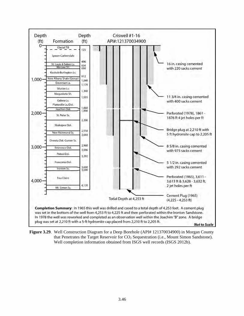
3.46
Figure 3.29. Well Construction Diagram for a Deep Borehole (API# 121370034900) in Morgan County that Penetrates the Target Reservoir for CO2 Sequestration (i.e., Mount Simon Sandstone). Well completion information obtained from ISGS well records (ISGS 2012b).
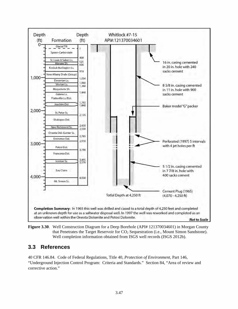
3.47
Figure 3.30. Well Construction Diagram for a Deep Borehole (API# 121370034601) in Morgan County that Penetrates the Target Reservoir for CO2 Sequestration (i.e., Mount Simon Sandstone). Well completion information obtained from ISGS well records (ISGS 2012b).
3.3 References
40 CFR 146.84. Code of Federal Regulations, Title 40, Protection of Environment, Part 146, “Underground Injection Control Program: Criteria and Standards.” Section 84, “Area of review and corrective action.”

3.48
75 FR 77230. December 10, 2010. “Federal Requirements Under the Underground Injection Control (UIC) Program for Carbon Dioxide (CO2) Geologic Sequestration (GS) Wells.” Federal Register. Environmental Protection Agency.
Akaike H. 1974. “A New Look at Statistical-Model Identification.” IEEE Automat. Contr. Ac19(6):716-723.
Birkholzer JT, J Apps, L Zhenge, Y Zhang, T Xu and C Tzang. 2008. Research Project on CO2
Geological Storage and Groundwater Resources: Large-Scale Hydrological Evaluation and Modeling of the Impact on Groundwater Systems Annual Report: October 1, 2007, to September 30, 2008. Lawrence Berkeley National Laboratory, Berkeley, California.
Buschbach TC and DC Bond. 1974. Underground Storage of Natural Gas in Illinois − 1973. Illinois Petroleum 101, Illinois State Geological Survey, Champaign, Illinois.
Davies PB. 1991. Evaluation of the Role of Threshold Pressure in Controlling Flow of Waste-Generated Gas into Bedded Salt at the Waste Isolation Pilot Plant (WIPP). SAND 90-3246, Sandia National Laboratory, Albuquerque, New Mexico.
EPA (U.S. Environmental Protection Agency). 2011a. Draft Underground Injection Control (UIC) Program Class VI Well Area of Review Evaluation and Corrective Action Guidance for Owners and Operators. EPA 816-D-10-007, EPA Office of Water, Washington, D.C.
EPA (U.S. Environmental Protection Agency). 2011b. “Underground Injection Control Permit Application IL-ICCS Project.” Administrative Record for Underground Injection Control Permit Application from Archer Daniels Midland Company, EPA Region 5, Chicago Illinois.
EPA (U.S. Environmental Protection Agency). 2011c. “Underground Injection Control Permit Application IL-ICCS Project.” Administrative Record for Underground Injection Control Permit Application from Christian County Generation, LLC of Taylorville, EPA Region 5, Chicago Illinois.
EPA (U.S. Environmental Protection Agency). 1994. “Determination of Maximum Injection Pressure for Class I Wells.” Underground Injection Control Section Regional Guidance #7. EPA Region 5, Chicago, Illinois.
Haimson BC and FH Cornet. 2003. "ISRM Suggested Methods for rock stress estimation—Part 3: hydraulic fracturing (HF) and/or hydraulic testing of pre-existing fractures (HTPF)." International Journal of Rock Mechanics and Mining Sciences 40(7–8):1011-1020.
Hornung J and T Aigner. 1999. "Reservoir and aquifer characterization of fluvial architectural elements: Stubensandstein, Upper Triassic, southwest Germany." Sedimentary Geology 129(3–4):215-280.
Hou Z, ML Rockhold, and CJ Murray. 2012. “Evaluating the impact of caprock and reservoir properties on potential risk of CO2 leakage after injection.” Environmental Earth Sciences 66(8):2403-2415, doi:10.1007/s12665-011-1465-2.
Hubbert MK and DG Willis. 1957. “Mechanics of hydraulic fracturing.” Petroleum Transactions, AIME, 210:153-168.
3.49
ISGS (Illinois State Geological Survey). 2012a. ILWATER Interactive Mapping Web Interface. Last accessed on January 4, 2012 at http://www.isgs.illinois.edu/maps-data-pub/wwdb/launchims.shtml.
ISGS (Illinois State Geological Survey). 2012b. Geologic Records Unit (GRU) Website. Last accessed on February 16, 2012 at http://www.isgs.uiuc.edu/sections/oil-gas/launchims.shtml.
ISGS (Illinois State Geological Survey). 2011. Illinois Oil and Gas Resources (ILOIL) Internet Map Service. Last accessed on October 8, 2011 at http://moulin.isgs.uiuc.edu/ILOIL/webapp/ILOIL.html
Kerr DR, L Ye, A Bahar, BM Kelkar, and S Montgomery. 1999. “Glenn Pool Field, Oklahoma: A Case of Improved Production from a Mature Reservoir.” American Association of Petroleum Geologists Bulletin 83(1):1-18.
Meyer R and FF Krause. 2006. "Permeability Anisotropy and Heterogeneity of a Sandstone Reservoir Analogue: An Estuarine to Shoreface Depositional System in the Virgelle Member, Milk River Formation, Writing-On-Stone Provincial Park, Southern Alberta." Bulletin of Canadian Petroleum Geology 54(4):301-318.
Pruess K, J Garcia, T Kovscek, C Oldenburg, J Rutqvist, C Steefel, and T Xu. 2002. Intercomparison of Numerical Simulation Codes for Geologic Disposal of CO2. LBNL-51813, Lawrence Berkeley National Laboratory, Berkeley, California.
Ringrose P, K Nordahl, and RJ Wen. 2005. "Vertical permeability estimation in heterolithic tidal deltaic sandstones." Petroleum Geoscience 11(1):29-36.
Saller AH, J Schwab, S Walden, S Robertson, R Nims, H Hagiwara, and S Mizohata. 2004. “Three-dimensional seismic imaging and reservoir modeling of an upper Paleozoic “reefal” buildup, Reinecke Field, west Texas, United States.” Pp. 107-125 in GP Eberli, JL Masaferro, and JF Sarg (eds.), Seismic Imaging of Carbonate Reservoirs and Systems, Volume 81, American Association of Petroleum Geologists, Tulsa, Oklahoma.
Span R and W Wagner. 1996. “A New Equation of State for Carbon Dioxide Covering the Fluid Region from the Triple-Point Temperature to 1100 K at Pressures Up to 800 MPa.” J Phys Chem Ref Data 25:1509-1596.
Spycher N and K Pruess. 2010. “A Phase-Partitioning Model for CO2-Brine Mixtures at Elevated Temperatures and Pressures: Application to CO2-Enhanced Geothermal Systems.” Transport in Porous Media 82:173-196. doi:10.1007/s11242-009-9425-y.
Spycher N, K Pruess, and J Ennis-King. 2003. “CO2-H2O mixtures in geological sequestration of CO2. I. Assessment and calculation of mutual solubilities from 12 to 100°C and up to 600 bar.” Geochimica et Cosmoschimica Acta 67(16):3015-3031. doi:10.1016/s0016-7037(03)00273-4.
Suekane T, NH Thanh, T Matsumoto, M Matsuda, M Kiyota, and A Ousaka. 2009. “Direct measurement of trapped gas bubbles by capillarity on the pore scale.” Energy Procedia 1(1):3189-3196, doi:10.1016/j.egypro.2009.02.102.

3.50
Venables WN and BD Ripley. 2002. Modern applied statistics with S. Springer Science+Business Media, NewYork, New York.
White MD, DH Bacon, BP McGrail, DJ Watson, SK White, and ZF Zhang. 2012. STOMP Subsurface Transport Over Multiple Phases: STOMP-CO2 and STOMP-CO2e Guide, Version 1.0. PNNL-21268, Pacific Northwest National Laboratory, Richland, Washington.
White MD and M Oostrom. 2006. STOMP Subsurface Transport Over Multiple Phases, Version 4: User's Guide. PNNL-15782, Pacific Northwest National Laboratory, Richland, Washington.
White MD and M Oostrom. 2000. STOMP Subsurface Transport Over Multiple Phases: Theory Guide. PNNL-12030, Pacific Northwest National Laboratory, Richland, Washington.
Zhou Q, JT Birkholzer, E Mehnert, Y-F Lin, and K Zhang. 2010. “Modeling basin- and plume-scale processes of CO2 storage for full-scale deployment.” Ground Water 48(4):494–514.
Zoback MD, CA Barton, M Brudy, DA Castillo, T Finkbeiner, BR Grollimund, DB Moos, P Peska, CD Ward, and DJ Wiprut. 2003. "Determination of stress orientation and magnitude in deep wells." International Journal of Rock Mechanics and Mining Sciences 40(7–8):1049-1076.