3.0 Sampling Plan Development Within VSP · 3.0 Sampling Plan Development Within VSP ... toward a complete set of sampling design ... according to some characteristic or feature of

3.0 Sampling Plan Development Within VSP

3.1 Sampling Plan Type Selection

Sampling plan components consist of where to take samples, how many samples to take, what kind of samples (e.g., surface soil, air), and how to take samples and analyze them. We identified the general areas of where to take samples in Section 2.3, Sample Areas in VSP. In this section, we discuss where within the Sampling Area to locate the samples. We also discuss how many samples to take. The kind of samples to take—i.e., soil vs. groundwater, wet vs. dry, surface vs. core,—is determined during Step 3 of the DQO process (Define Inputs) and is not addressed directly in VSP. The Measurement Quality Objectives module in VSP (Section 5.4) deals with how the method selected for analytically measuring the sample relates to other components of the sampling plan.

3.1.1 Defining the Purpose/Goal of Sampling

VSP follows the DQO planning process in directing users in the selection of the components of the sampling plan. The first thing you must do is to select the type of problem for which the current data collection effort will be used to resolve. In VSP, we call this the Sampling Goal. The following types of problems are addressed currently in VSP. Future versions will expand on this list:

Sampling Goal Description Compare Average to Fixed Threshold Calculates number of samples needed to compare a sample mean or

median against a predetermined threshold and places them on the map. This is called a one-sample problem

Compare Average to Reference Average Calculates number of samples needed to compare a sample mean or median against a reference mean or median and places them on the map. This is typically used when a reference area has been selected (i.e., a background area) and the problem is to see if the study area is equal to, or greater than, the reference area. This is called a two-sample problem because the data from two sites are compared to each other

Estimate the Mean Calculates number of samples needed to estimate the population mean and places them on the map

Construct Confidence Interval on Mean Calculates number of samples needed to find a confidence interval on a mean and places them on the map

Compare Proportion to Fixed Threshold Calculates number of samples needed to compare a proportion to a given proportion and places them on the map

Compare Proportion to Reference Proportion Calculates number of samples needed to compare two proportions and places them on the map

Estimate the Proportion Calculates number of samples needed to estimate the population proportion and places them on the map.

Locating a Hot Spot Use systematic grid sampling to locate a Hot Spot (i.e., small pockets of contamination).

Find UXO Target Areas Traverse and detect an elliptical target zone using swath sampling. Calculates spacing for swaths. Evaluates post-survey target detection.

Assess Degree of Confidence in UXO Presence Assess degree of confidence in UXO presence. Non-statistical sampling approach Allows samples to be added to the map without the guidance of

statistical methods. Establish boundary of Contamination Determine whether contamination has migrated across the boundary. Sampling within a Building Allows sampling within rooms, zones, floors, etc., for various

contamination release scenarios and end goals.

July 2005 Visual Sample Plan Version 4.0 3.1

This list of sampling goals available now in VSP reflects the targeted interests and specific problems of our current VSP sponsors. Therefore, the available sampling designs within VSP are not an exhaustive list of designs you might find in a commercial statistical sampling package. Future versions will work toward a complete set of sampling design offerings.

VSP lists “Non-statistical sampling approach” under Sampling Goals, but this is not really a goal. Under this category, VSP allows the user to specify a predetermined sample size and locate the samples judgmentally. Because VSP has no way of knowing how the sample size and sample locations were chosen, the sampling approach is considered to be “non-statistical” (i.e., no confidence can be assigned to the conclusions drawn from judgment samples).

To give you an idea of how VSP threads from Sampling Goal to selection of a sampling design, Figure 3.1 shows the sequence of pull-down menus for one of the goals, Compare Average to a Fixed Threshold. All endpoints from the Sampling Goal main menu result in a dialog box where the user provides inputs for the specific design selected. VSP allows only certain options and designs (e.g., simple random, systematic) under each goal. This is because VSP contains the algorithms for calculating sample number and locating samples for only certain goal-assumptions-statistical test or method sequences. Future versions of VSP will expand on the number and type of algorithms offered.

Figure 3.1. Menu Options in VSP for Compare Average to Fixed Threshold

Visual Sample Plan Version 4.0 July 2005 3.2

3.1.2 Selecting a Sampling Design

The current release of VSP offers several versions of the software (see Figure 2.1). Each version has a unique set of sampling designs available to the user – except General (all inclusive) VSP which contains all the designs. Some of the designs available under each of the Sampling Goal menu items are unique to that goal, other designs are available under multiple goals. Thus, the Sampling Goal you select determines which sampling design(s) will be available to you.

If a user is new to VSP, and is not looking for a specific sample design but rather has a general definition of the problem to be resolved with sample data, a good discussion of how to select a sampling design is in EPA’s Guide for Choosing a Sampling Design for Environmental Data Collection (EPA 2001) http://www.epa.gov/quality/qa_docs.html. See Table 3-1 on pages 23-24 in that source for examples of problem types that one may encounter and suggestions for sampling designs that are relevant for these problem types in particular situations. Another guidance document, Multi-Agency Radiation Survey and Site Investigation Manual (MARSSIM) (EPA 1997) http://www.epa.gov/radiation/marssim/, also provides insight into how to select a sample design.

One of the valuable ways to use VSP is to run through the various Goals and see what changes from one Goal to another, what sampling designs are available for each Goal, how designs perform, and what assumptions are required for each design. This trial and error approach is probably the best way to select a design that best fits your regulatory environment, unique site conditions, and goals.

An important point to keep in mind is the linkage between 1) the minimum number of samples that must be collected and where they are located, and 2) how you will analyze the sampling results to calculate summary values (on which you will base your decisions). The user must understand this linkage in order to select the appropriate design. Once the samples are collected and analyzed, the statistical tests and methods assumed in the sample size formulas and design must be used in the analysis phase, Data Quality Assessment (DQA).

Many of the designs in VSP contain a Data Analysis tab and require sample results to be input into VSP so tests can be executed and conclusions drawn based on the results. See Section 5.6 for a discussion of Data Analysis within VSP.

We cannot discuss all the technical background behind the designs here, but the technical documentation for VSP gives sample size formulas used in VSP and provides references. The VSP web site lists the technical documentation available, and allows download of the documents http://dqo.pnl.gov/VSP/documentation. The online help in VSP also provides technical help and references. Finally, the reports that are available within VSP are a good source for definitions, assumptions, sample size formulas, and technical justification for the design selected.

VSP allows both probability-based designs and judgmental sampling:

Probability-based sampling designs apply sampling theory and involve random selection. An essential feature of a probability-based sample is that each member of the population from which the sample was selected has a known probability of selection. When a probability based design is used, statistical inferences may be made about the sampled population from the data obtained


http://www.epa.gov/quality/qa_docs.html

http://www.epa.gov/radiation/marssim/

http://dqo.pnl.gov/VSP/documentation

from the sampled units. Judgmental designs involve the selection of sampling units on the basis of expert knowledge or professional judgment (EPA 2001, pp. 9-10).

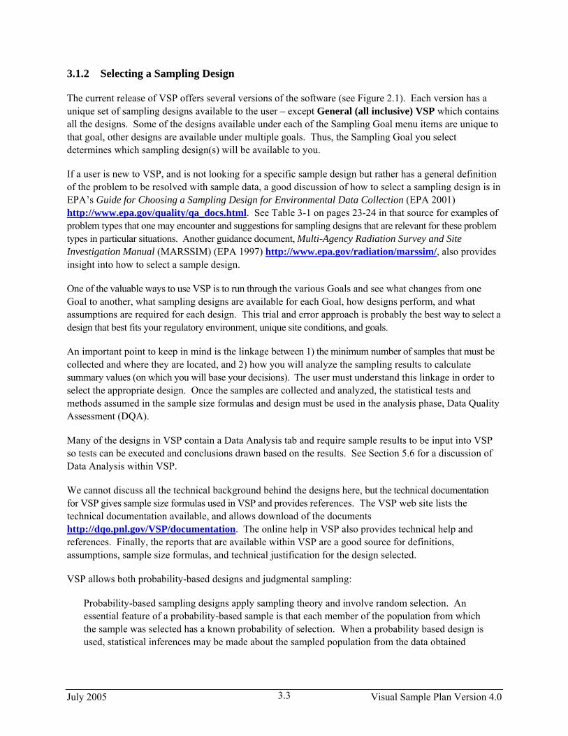
The design recommended by VSP depends on the sampling goal selected, assumptions made, and in the case of Ordinary Sampling, user input provided under the Sample Placement tab. VSP contains the following two- and three-dimensional designs. With exception to judgment sampling, these are probability-based designs.

• Ordinary sampling – two Sample Placement options are available:

1. simple random sampling where sampling locations are selected based on random numbers, which are then mapped to the spatial locations, and

2. systematic grid sampling where sampling locations are selected on a regular pattern (e.g., on a square grid, on a triangular grid, along a line) with the starting location randomly selected. Sampling is done only at the node points of the grid. The grid pattern is selected under Grid Type. Figure 3.2 shows the dialog box for making input selections. You can see an example of the grid pattern selected in red to the right of the Grid Type options. You may specify Random Start or a fixed start for the initial grid point using the check box next to Random Start. Choosing Random Start will generate a new random starting location for the first grid location each time the Apply button is pushed. Once all selections have been made, press Apply.

Figure 3.2. Sample Placement Tab for Ordinary Sampling for Selecting Sample Placement Method and Type


• stratified sampling – Strata or partitions of an area are made based on a set of criteria, such as homogeneity of contamination. Samples are drawn from each stratum according to a formula that accords more samples to more heterogeneous strata.

• adaptive cluster sampling – An initial n samples are selected randomly. Additional samples are taken at locations surrounding the initial samples where the measurements exceed some threshold value. Several rounds of sampling may be required. Selection probabilities are used to calculate unbiased estimates to compensate for oversampling in some areas.

• sequential sampling - Sequential designs are by their nature iterative, requiring the user to take a few samples (randomly placed) and enter the results into the program before determining whether further sampling is necessary to meet the sampling objectives.

• collaborative sampling - The Collaborative Sampling (CS) design , also called “double sampling”, uses two measurement techniques to obtain an estimate of the mean – one technique is the regular analysis method (usually more expensive), the other is inexpensive but less accurate. CS is not a type of sampling design but rather method for selecting which samples are analyzed by which measurement method.

• ranked set sampling – In this two-phased approach, sets of population units are selected and ranked according to some characteristic or feature of the units that is a good indicator of the relative amount of the variable or contaminant of interest that is present. Only the mth ranked unit is chosen from this set and measured. Another set is chosen, and the m-1th ranked unit is chosen and measured. This is repeated until the set with the unit ranked first is chosen and measured. The entire process is repeated for r cycles. Only the m X r samples are used to estimate an overall mean.

• sampling along a swath or transect – Continuous sampling is done along straight lines (swaths) of a certain width using geophysical sensors capable of continuous detection. Swath patterns can be parallel, square, or rectangular. The goal is to find circular or elliptical targets. This design contains the two elements of traversing the target and detecting the target. VSP application is for unexploded ordnance (UXO).

• sampling along a boundary - This design places samples along a boundary in segments, combines the samples for a segment, and analyzes each segment to see if contamination has spread beyond the boundary. If contamination has spread, VSP keeps extending the boundary until the sampling goals have been met.

• judgment sampling – You simply point and click anywhere in a sampling area. These sampling locations are based on the judgment of the user.

Because judgment sampling is not probability-based, users can bias the sampling results using this method. There is no basis in statistical theory for making confidence statements about conclusions drawn when samples are selected by judgment. However, some problem definitions might call for judgment sampling, such as looking in the most likely spot for evidence of contamination or taking samples at predefined locations. Figure 3.3 shows judgment sampling selected in VSP and six sampling locations selected manually.


(b)

(a)

Figure 3.3. Judgment Sampling in VSP

3.2 DQO Inputs and Sample Size

The inputs needed for VSP’s sample-size calculations are decided upon during the DQO process. If you have not gone through the DQO process prior to entering this information, you can enter “best guess” values for each of the inputs and observe the resulting computed sample size. New inputs can be tried until a sample size that is feasible and/or within budget is obtained. This iterative method for using VSP is a valuable “what if” tool with which you can see the effect on sample size (and hence costs) of changing DQO inputs. However, be cautioned that all the DQO elements interact and have special meaning within the context of the problem. To be able to defend the sample size that VSP calculates, you must have a defensible basis for each of the inputs. There is no quick way to generate this defense other than going through Steps 1 through 6 of the DQO process.

The core set of DQO inputs that affect sample size for most of the designs are as follows:

• Null Hypothesis Formulation – The null hypothesis is the working hypothesis or baseline condition of the environment. There must be convincing evidence in the data to declare the baseline condition to be false. VSP uses a default of “Site is Dirty” as the working hypothesis that must be disproved with convincing evidence from the data.


• Type I Error Rate (Alpha) – This is called the false rejection rate in EPA’s DQO guidance (EPA 2000a). This is the probability of rejecting a true null hypothesis. For the typical hypothesis test in which we assume the survey unit is dirty (above the action level), alpha is the chance a dirty site with a true mean equal to or greater than the Action Level will be released as clean to the public. In general, alpha is the maximum chance, assuming the DQO inputs are true, that a dirty site will be released as clean.

• Type II Error Rate (Beta) – This is called the false acceptance rate in EPA’s DQO guidance. This is the probability of not rejecting (accepting) a false null hypothesis. For the typical hypothesis test in which we assume the survey unit is dirty, beta is the chance a specific clean site will be condemned as dirty. Specifically, beta is the chance that a clean site with a true mean equal to or less than the lower bound of the gray region will be condemned as dirty. In general, beta is the maximum chance, outside the gray region, that a clean site will be condemned as dirty.

• Width of Gray Region (Delta) – This is the distance from the Action Level to the outer bound of the gray region. For the typical hypothesis test in which we assume the survey unit is dirty, the gray region can be thought of as a range of true means where we are willing to decide that clean sites are dirty with high probability. Typically, these probabilities are 20% to 95%, i.e., from beta to 1 - alpha. If this region is reduced to a very small range, the sample size grows to be extremely large. Determining a reasonable value for the size of the gray region calls for professional judgment and cost/benefit evaluation.

• Estimated Sampling Standard Deviation – This is an estimate of the standard deviation expected between the multiple samples. This estimate could be obtained from previous studies, previous experience with similar sites and contaminants, or expert opinion. Note that this is the square root of the variance. In one form or another, all the designs require some type of user-input as to the variability of contamination expected in the study area. After all, if the area to be sampled was totally homogeneous, only one sample would be required to completely characterize the area.

Other inputs are required by some of the designs, and other inputs are required for design parameters other than sample size. For example, the stratified designs require the user to specify the desired number of strata and estimates of proportions or standard deviations for each of the stratum. The UXO (unexploded ordinance) modules use Bayesian methods and require the user to input their belief that the study area contains UXO. When simulations are used, as in the post-survey UXO target detection, the user must input assumptions about distribution of scrap or shrapnel in the target areas. In the discussions of the designs, we try to give an explanation of each input required of the user. If you are lost, use the VSP Help functions (See Section 2.7).

Note: The Help Topics function in VSP provides a description of each of the designs and its related inputs. You can also select the Help button on the toolbar, put the cursor on any of the designs on the menu and a description of the design and its inputs will appear in a Help window. In addition, pressing the Help button at the bottom of each design dialog will bring up a Help window that contains a complete explanation of the design. Finally, on each screen where input is required, highlight an item and press the F1 key for a description of that input item.

The next section contains a discussion of the inputs required by most of the designs available in the current release of VSP. The designs are organized by the Sampling Goal under which they fall. Not all options



for all designs are discussed. Common design features (such as Costs, Historical Samples, MQO) that are found in multiple designs will not be discussed individually in this section but can be found in Section 5.0, Extended Features of VSP.

3.2.1 Compare Average to a Fixed Threshold

Comparing the average to a fixed threshold is the most common problem confronted by environmental remediation engineers. We present different forms the problem might take and discuss how VSP can be used to address each problem formulation.

We can continue where we left off in Section 2.3.3 with the Millsite.dxf map loaded. We selected a single Sample Area from the site. The Action Level for the contaminant of interest is 6 pCi/g in the top 6 in. of soil. Previous investigations indicate an estimated standard deviation of 2 pCi/g for the contaminant of interest. The null hypothesis for this problem is “Assume Site is Dirty” or HO: True mean ≥ A.L.

We desire an alpha error rate of 1% and a beta error rate of 1%. According to EPA (2000a, pp. 6-10), 1% for both alpha and beta are the most stringent limits on decision errors typically encountered for environmental data. We tentatively decide to set the lower bound of the gray region at 5 pCi/g and decide a systematic grid is preferable.

We will use VSP to determine the final width of the gray region and the number of samples required. Assume the fixed cost of planning and validation is $1,000, the field collection cost per sample is $100, and the laboratory analytical cost per sample is $400. We are told to plan on a maximum sampling budget of $20,000.

Case 1: We assume that the population from which we are sampling is approximately normal or that it is well-behaved enough that the Central Limit Theorem of statistics applies. In other words, the distribution of sample means drawn from the population is approximately normally distributed. We also decided that a systematic pattern for sample locations is better than a random pattern because we want complete coverage of the site.

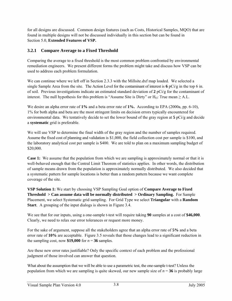
VSP Solution 1: We start by choosing VSP Sampling Goal option of Compare Average to Fixed Threshold > Can assume data will be normally distributed > Ordinary Sampling. For Sample Placement, we select Systematic grid sampling. For Grid Type we select Triangular with a Random Start. A grouping of the input dialogs is shown in Figure 3.4.

We see that for our inputs, using a one-sample t-test will require taking 90 samples at a cost of $46,000. Clearly, we need to relax our error tolerances or request more money.

For the sake of argument, suppose all the stakeholders agree that an alpha error rate of 5% and a beta error rate of 10% are acceptable. Figure 3.5 reveals that those changes lead to a significant reduction in the sampling cost, now $19,000 for n = 36 samples.

Are these new error rates justifiable? Only the specific context of each problem and the professional judgment of those involved can answer that question.

What about the assumption that we will be able to use a parametric test, the one-sample t-test? Unless the population from which we are sampling is quite skewed, our new sample size of n = 36 is probably large

(c)

(a) (b)

Figure 3.4. Input Boxes for Case 1 with Original Error Rates

July 2005 3.9

Visual Sam

ple Plan Version 4.0

Figure 3.5. Input Boxes for Case 1 with Increased Error Rates

enough to justify using a parametric test. Of course, once we take the data, we will need to justify our assumptions as pointed out in Guidance for Data Quality Assessment Practical Methods for Data Analysis (EPA 2000b, pp. 3-5).

Case 2: We now decide that we want to look at designs that may offer us cost savings over the systematic design just presented. We have methods available for collecting and analyzing samples in the field making quick turnaround possible. We want to be efficient and cost-effective and take only enough samples to confidently say whether our site is clean or dirty. After all, if our first several samples exhibit


levels of contamination so high that there is no possible scenario for the average to be less than a threshold, why continue to take more samples? We can make a decision right now that the site needs to be remediated. Sequential designs, and the tests associated with them, take previous sampling results into account and provide rules specifying when sampling can stop and a decision can be made.

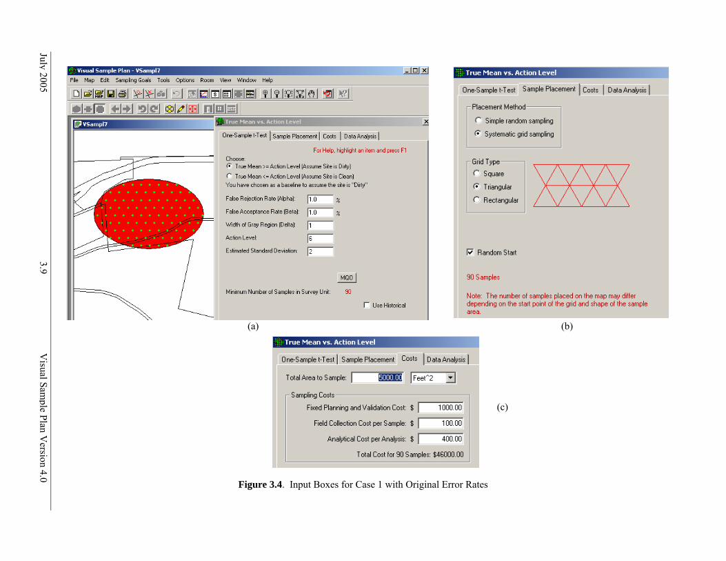
VSP Solution 2a: From VSP’s main menu, select Sampling Goal of Compare Average to a Fixed Threshold > Can assume data will be normally distributed > Sequential Sampling (Known Standard Deviation). The dialog box in Figure 3.6 appears. We begin by entering the DQO parameters for Alpha, Beta, Action Level, etc. Next, enter the Number of Samples Per Round, shown here as 3. This parameter indicates how many samples you want to take each time you mobilize into the field. Each time you press the Apply button, VSP places a pattern of this many sampling locations on the map.

When you close this design dialog, this pattern of sampling locations is locked or “frozen.” In Figure 3.6, we see the results of pressing Apply, and three locations are placed on the Map labeled “Seq-1, Seq-2, Seq 3”.

You must now exit this dialog (close the display by clicking the X in the upper right-hand corner of the display), go out and take the samples, and analyze them. Once the sample results are available, re-open the

Figure 3.6. Dialog for Sequential Sampling (Standard Deviation Known) and Three Locations Placed on the Map


Sequential Probability Ratio Test (SPRT) design dialog box. The easiest way to re-open a sampling design, is to use the menu item: Sampling Goals > Last Design or click the Last Design button on the main toolbar.

Note: This is the case with all VSP modules where the user must input sampling results – you must exit the dialog box, enter the results, and re-enter the dialog box.

You now see the Number of Samples Collected as 3. Press the Input Values button and enter the measurement values for those three samples into the grid on the data input dialog. We enter these values as 6.5, 8, and 5. Press the OK button and VSP returns to the original SPRT dialog box. We now see that

VSP calculated a mean of 6.5 and a standard deviation of 1.5 for the values we entered. VSP cannot accept or reject the null hypothesis within the error limits we specified based on these values and suggests that 9 additional samples are needed to make a decision.

Figure 3.7. Data Input Dialog for Sequential Probability Ratio Test and Results from First Round of Sampling. Map View is shown in background.


Switching over to the Graph View in Figure 3.8, we can see that in order to accept the null hypothesis that the site is dirty by taking just three samples, we need a sample mean of approximately 9 (i.e., cross-hair set at 3 on the x-axis, intersects the lower boundary of the red area at 9 on the y-axis). If we move the cursor to the green area, the cross-hair intersects the upper boundary of the green area at approximately 2.5. In other words, we need a sample mean of 2.5 in order to reject the null hypothesis and declare the site clean with only three values. Remember, we told VSP that we knew the standard deviation to be 2, so that is what the program is using to make the projection of additional samples needed. If we are wrong, the VSP output will be misleading.

Figure 3.8. Graph View of Sequential Sampling

The two open circles in Figure 3.8 show the sample mean after the first two samples are collected. The closed circle shows the mean at the end of the third sample. We take the next set of three samples and get values 10, 5, and 12. VSP now tells us that we can Accept the Null Hypothesis and conclude the site is dirty.


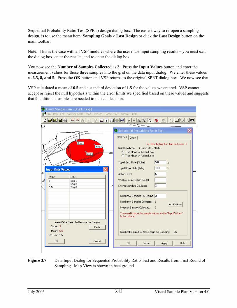
VSP Solution 2b: We now observe what happens when we do not know the true standard deviation of units in the population and select Sampling Goal of Compare Average to a Fixed Threshold > Can assume data will be normally distributed > Sequential Sampling (Unknown Standard Deviation). The dialog box that appears is for a different test, Barnard’s Sequential Test, shown in Figure 3.9. We enter the same DQO inputs of Alpha, Beta, Action Level, etc. We also say we will take 3 Samples Per Round. Using Barnard’s test, VSP tells us that we need to take at least 10 samples in order to make a decision. VSP places these 10 samples on the map.

Figure 3.9. Dialog Box for Sequential Sampling (Unknown Standard Deviation)

VSP Solution 2c. We have one other option for more cost-efficient sampling – reduce the analytic laboratory costs by taking advantage of measurement equipment that may be less accurate, but is less


expensive. If we can still meet our DQOs (error levels, width of grey region) taking advantage of the less expensive equipment, we will save money.

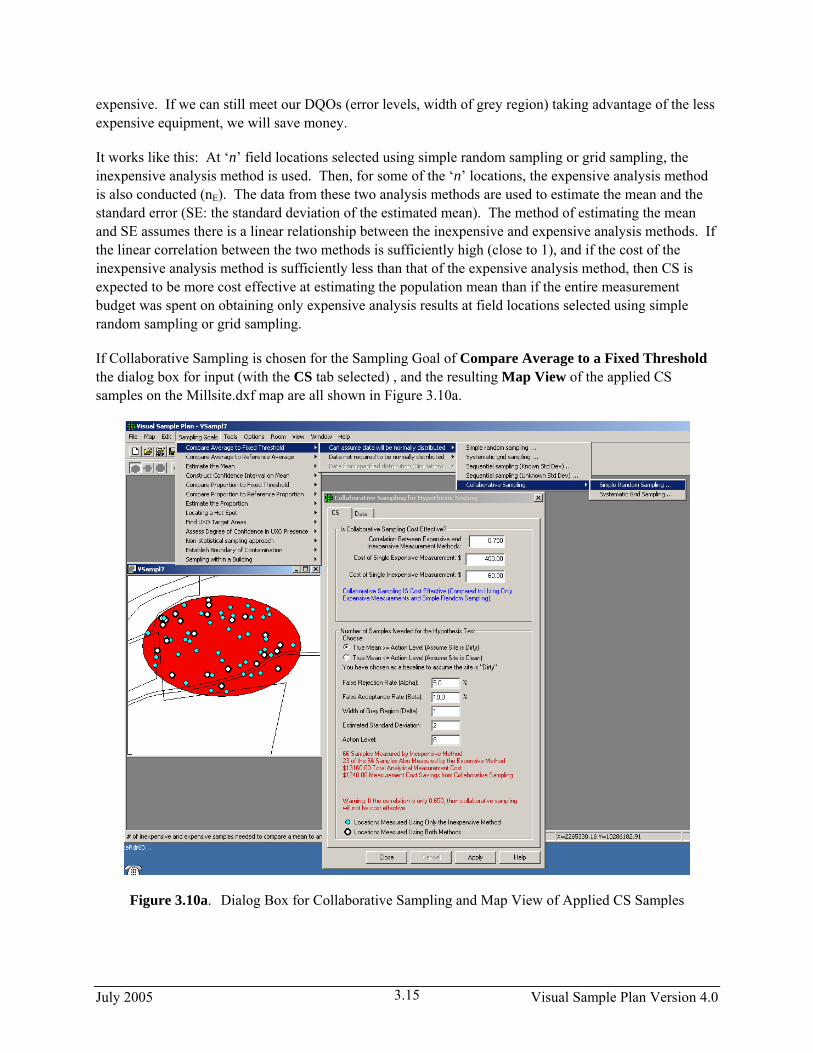
It works like this: At ‘n’ field locations selected using simple random sampling or grid sampling, the inexpensive analysis method is used. Then, for some of the ‘n’ locations, the expensive analysis method is also conducted (nE). The data from these two analysis methods are used to estimate the mean and the standard error (SE: the standard deviation of the estimated mean). The method of estimating the mean and SE assumes there is a linear relationship between the inexpensive and expensive analysis methods. If the linear correlation between the two methods is sufficiently high (close to 1), and if the cost of the inexpensive analysis method is sufficiently less than that of the expensive analysis method, then CS is expected to be more cost effective at estimating the population mean than if the entire measurement budget was spent on obtaining only expensive analysis results at field locations selected using simple random sampling or grid sampling.

If Collaborative Sampling is chosen for the Sampling Goal of Compare Average to a Fixed Threshold the dialog box for input (with the CS tab selected) , and the resulting Map View of the applied CS samples on the Millsite.dxf map are all shown in Figure 3.10a.

Figure 3.10a. Dialog Box for Collaborative Sampling and Map View of Applied CS Samples


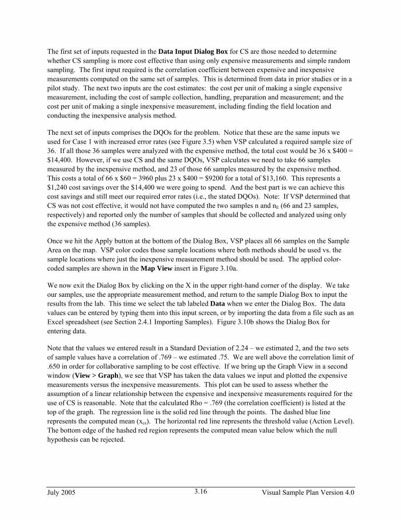
The first set of inputs requested in the Data Input Dialog Box for CS are those needed to determine whether CS sampling is more cost effective than using only expensive measurements and simple random sampling. The first input required is the correlation coefficient between expensive and inexpensive measurements computed on the same set of samples. This is determined from data in prior studies or in a pilot study. The next two inputs are the cost estimates: the cost per unit of making a single expensive measurement, including the cost of sample collection, handling, preparation and measurement; and the cost per unit of making a single inexpensive measurement, including finding the field location and conducting the inexpensive analysis method.

The next set of inputs comprises the DQOs for the problem. Notice that these are the same inputs we used for Case 1 with increased error rates (see Figure 3.5) when VSP calculated a required sample size of 36. If all those 36 samples were analyzed with the expensive method, the total cost would be 36 x $400 = $14,400. However, if we use CS and the same DQOs, VSP calculates we need to take 66 samples measured by the inexpensive method, and 23 of those 66 samples measured by the expensive method. This costs a total of 66 x $60 = 3960 plus 23 x $400 = $9200 for a total of $13,160. This represents a $1,240 cost savings over the $14,400 we were going to spend. And the best part is we can achieve this cost savings and still meet our required error rates (i.e., the stated DQOs). Note: If VSP determined that CS was not cost effective, it would not have computed the two samples n and nE (66 and 23 samples, respectively) and reported only the number of samples that should be collected and analyzed using only the expensive method (36 samples).

Once we hit the Apply button at the bottom of the Dialog Box, VSP places all 66 samples on the Sample Area on the map. VSP color codes those sample locations where both methods should be used vs. the sample locations where just the inexpensive measurement method should be used. The applied color-coded samples are shown in the Map View insert in Figure 3.10a.

We now exit the Dialog Box by clicking on the X in the upper right-hand corner of the display. We take our samples, use the appropriate measurement method, and return to the sample Dialog Box to input the results from the lab. This time we select the tab labeled Data when we enter the Dialog Box. The data values can be entered by typing them into this input screen, or by importing the data from a file such as an Excel spreadsheet (see Section 2.4.1 Importing Samples). Figure 3.10b shows the Dialog Box for entering data.

Note that the values we entered result in a Standard Deviation of 2.24 – we estimated 2, and the two sets of sample values have a correlation of .769 – we estimated .75. We are well above the correlation limit of .650 in order for collaborative sampling to be cost effective. If we bring up the Graph View in a second window (View > Graph), we see that VSP has taken the data values we input and plotted the expensive measurements versus the inexpensive measurements. This plot can be used to assess whether the assumption of a linear relationship between the expensive and inexpensive measurements required for the use of CS is reasonable. Note that the calculated Rho = .769 (the correlation coefficient) is listed at the top of the graph. The regression line is the solid red line through the points. The dashed blue line represents the computed mean (xcs). The horizontal red line represents the threshold value (Action Level). The bottom edge of the hashed red region represents the computed mean value below which the null hypothesis can be rejected.


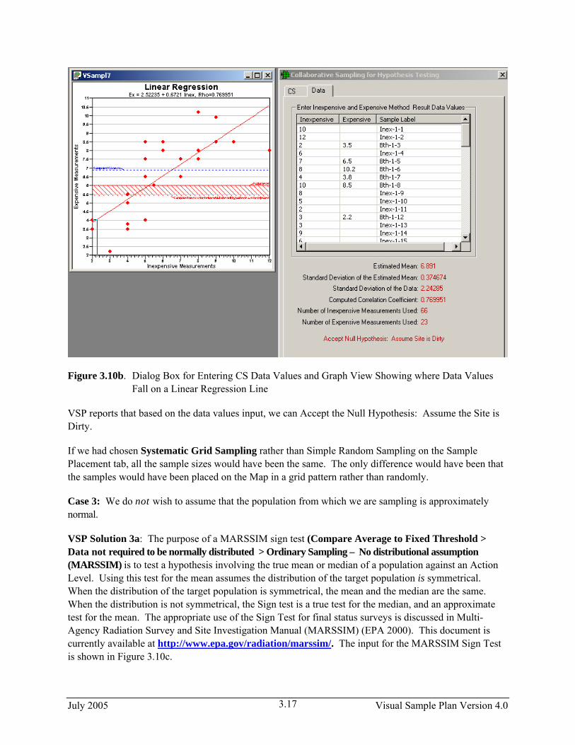
Figure 3.10b. Dialog Box for Entering CS Data Values and Graph View Showing where Data Values Fall on a Linear Regression Line

VSP reports that based on the data values input, we can Accept the Null Hypothesis: Assume the Site is Dirty.

If we had chosen Systematic Grid Sampling rather than Simple Random Sampling on the Sample Placement tab, all the sample sizes would have been the same. The only difference would have been that the samples would have been placed on the Map in a grid pattern rather than randomly.

Case 3: We do not wish to assume that the population from which we are sampling is approximately normal.

VSP Solution 3a: The purpose of a MARSSIM sign test (Compare Average to Fixed Threshold > Data not required to be normally distributed > Ordinary Sampling – No distributional assumption (MARSSIM) is to test a hypothesis involving the true mean or median of a population against an Action Level. Using this test for the mean assumes the distribution of the target population is symmetrical. When the distribution of the target population is symmetrical, the mean and the median are the same. When the distribution is not symmetrical, the Sign test is a true test for the median, and an approximate test for the mean. The appropriate use of the Sign Test for final status surveys is discussed in Multi-Agency Radiation Survey and Site Investigation Manual (MARSSIM) (EPA 2000). This document is currently available at http://www.epa.gov/radiation/marssim/. The input for the MARSSIM Sign Test is shown in Figure 3.10c.



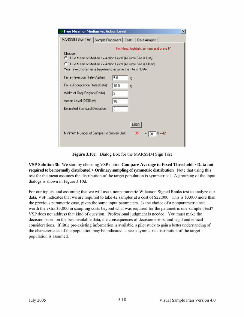
Figure 3.10c. Dialog Box for the MARSSIM Sign Test

VSP Solution 3b: We start by choosing VSP option Compare Average to Fixed Threshold > Data not required to be normally distributed > Ordinary sampling of symmetric distribution. Note that using this test for the mean assumes the distribution of the target population is symmetrical. A grouping of the input dialogs is shown in Figure 3.10d.

For our inputs, and assuming that we will use a nonparametric Wilcoxon Signed Ranks test to analyze our data, VSP indicates that we are required to take 42 samples at a cost of $22,000. This is $3,000 more than the previous parametric case, given the same input parameters. Is the choice of a nonparametric test worth the extra $3,000 in sampling costs beyond what was required for the parametric one-sample t-test? VSP does not address that kind of question. Professional judgment is needed. You must make the decision based on the best available data, the consequences of decision errors, and legal and ethical considerations. If little pre-existing information is available, a pilot study to gain a better understanding of the characteristics of the population may be indicated, since a symmetric distribution of the target population is assumed.


Figure 3.10d. Input Dialog for Wilcoxon Signed Rank Test

3.2.2 Compare Average to Reference Average

We again start with the Millsite.dxf map from Section 2.3.3 with a single Sample Area defined. The Action Level for the contaminant of interest is 5 pCi/g above background in the top 6 in. of soil. Background is found by sampling an appropriate reference area. Previous investigations indicate an estimated standard deviation of 2 pCi/g for the contaminant of interest. The null hypothesis for this problem is “Assume Site is Dirty” or HO: Difference of True Means ≥ Action Level. In other words, the parameter of interest for this test is the difference of means, not an individual mean as was the case in the one-sample t-test.


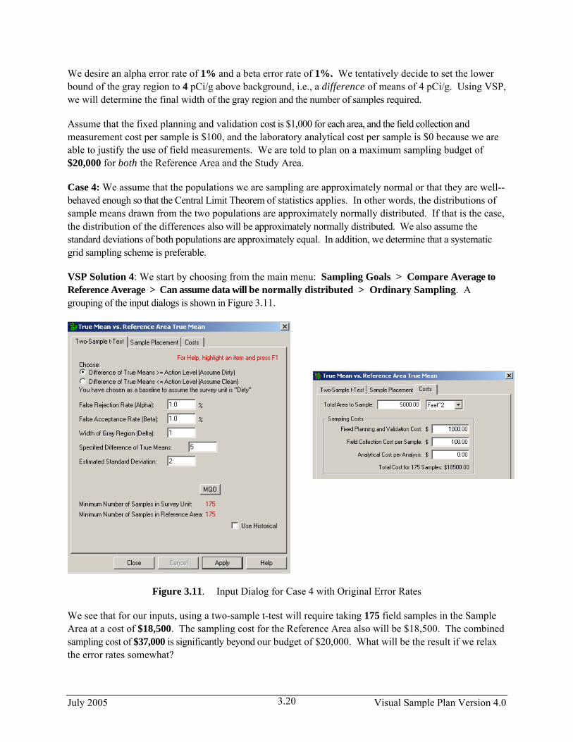
We desire an alpha error rate of 1% and a beta error rate of 1%. We tentatively decide to set the lower bound of the gray region to 4 pCi/g above background, i.e., a difference of means of 4 pCi/g. Using VSP, we will determine the final width of the gray region and the number of samples required.

Assume that the fixed planning and validation cost is $1,000 for each area, and the field collection and measurement cost per sample is $100, and the laboratory analytical cost per sample is $0 because we are able to justify the use of field measurements. We are told to plan on a maximum sampling budget of $20,000 for both the Reference Area and the Study Area.

Case 4: We assume that the populations we are sampling are approximately normal or that they are well--behaved enough so that the Central Limit Theorem of statistics applies. In other words, the distributions of sample means drawn from the two populations are approximately normally distributed. If that is the case, the distribution of the differences also will be approximately normally distributed. We also assume the standard deviations of both populations are approximately equal. In addition, we determine that a systematic grid sampling scheme is preferable.

VSP Solution 4: We start by choosing from the main menu: Sampling Goals > Compare Average to Reference Average > Can assume data will be normally distributed > Ordinary Sampling. A grouping of the input dialogs is shown in Figure 3.11.

Figure 3.11. Input Dialog for Case 4 with Original Error Rates

We see that for our inputs, using a two-sample t-test will require taking 175 field samples in the Sample Area at a cost of $18,500. The sampling cost for the Reference Area also will be $18,500. The combined sampling cost of $37,000 is significantly beyond our budget of $20,000. What will be the result if we relax the error rates somewhat?


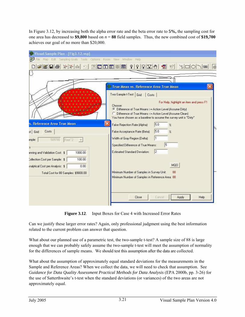
In Figure 3.12, by increasing both the alpha error rate and the beta error rate to 5%, the sampling cost for one area has decreased to $9,800 based on n = 88 field samples. Thus, the new combined cost of $19,700 achieves our goal of no more than $20,000.

Figure 3.12. Input Boxes for Case 4 with Increased Error Rates

Can we justify these larger error rates? Again, only professional judgment using the best information related to the current problem can answer that question.

What about our planned use of a parametric test, the two-sample t-test? A sample size of 88 is large enough that we can probably safely assume the two-sample t-test will meet the assumption of normality for the differences of sample means. We should test this assumption after the data are collected.

What about the assumption of approximately equal standard deviations for the measurements in the Sample and Reference Areas? When we collect the data, we will need to check that assumption. See Guidance for Data Quality Assessment Practical Methods for Data Analysis (EPA 2000b, pp. 3-26) for the use of Satterthwaite’s t-test when the standard deviations (or variances) of the two areas are not approximately equal.


Case 5: We now look at the case in which the nonparametric Wilcoxon Rank Sum (WRS) Test is planned for the data analysis phase of the project. VSP offers two versions of the WRS Test: the MARSSIM WRS test and the Wilcoxon Rank Sum Test. If the Sample and Reference population distributions are not symmetric, both WRS methods test the differences in the medians. If one wants to make a statement about the differences between means using the WRS tests, it is required that the two distributions be symmetric so that the mean equals the median. The verification testing done on VSP shows that the Wilcoxon rank sum test requires slightly higher sample sizes than the MARSSIM WRS test for the same set of inputs, assuming all the appropriate assumptions for each test are met.

The Wilcoxon rank sum test is discussed in Guidance for Data Quality Assessment (EPA 2000b, pp. 3-31 – 3-34). The document can be downloaded from the EPA at: http://www.epa.gov/quality/qa_docs.html. It tests a shift in the distributions of two populations. The two distributions are assumed to have the same shape and dispersion, so that one distribution differs by some fixed amount from the other distribution. The user can structure the null and alternative hypothesis to reflect the amount of shift of concern and the direction of the shift.

VSP Solution 5: We start by choosing from VSP’s main menu Sampling Goals > Compare Average to Reference Average > Data not required to be normally distributed > Ordinary sampling – no distributional assumption. A grouping of the input dialogs is shown in Figure 3.13.

Figure 3.13. Input Boxes for Case 5 Using Nonparametric Wilcoxon Rank Sum Test


http://www.epa.gov/quality/qa_docs.html

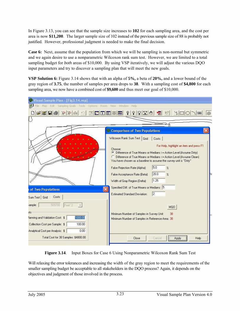
In Figure 3.13, you can see that the sample size increases to 102 for each sampling area, and the cost per area is now $11,200. The larger sample size of 102 instead of the previous sample size of 88 is probably not justified. However, professional judgment is needed to make the final decision.

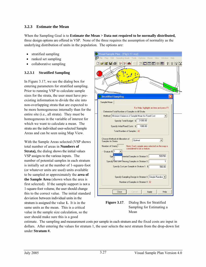
Case 6: Next, assume that the population from which we will be sampling is non-normal but symmetric and we again desire to use a nonparametric Wilcoxon rank sum test. However, we are limited to a total sampling budget for both areas of $10,000. By using VSP iteratively, we will adjust the various DQO input parameters and try to discover a sampling plan that will meet the new goals.

VSP Solution 6: Figure 3.14 shows that with an alpha of 5%, a beta of 20%, and a lower bound of the gray region of 3.75, the number of samples per area drops to 38. With a sampling cost of $4,800 for each sampling area, we now have a combined cost of $9,600 and thus meet our goal of $10,000.


Will relaxing the error tolerances and increasing the width of the gray region to meet the requirements of the smaller sampling budget be acceptable to all stakeholders in the DQO process? Again, it depends on the objectives and judgment of those involved in the process.


Case 7: Suppose our combined sampling budget is reduced to $5,000. Can VSP provide a sampling design that meets that goal?

VSP Solution 7: Figure 3.15 shows a design with just 14 samples per sampling area that meets the new sparse budget. We reduced the combined sampling cost, now $4,800, by increasing the width of the gray region to 2.1 pCi/g (lower bound of the gray region is 2.9 pCi/g).


There are definite consequences of reducing sampling requirements to fit a budget. The consequences could include a greater chance of concluding that a dirty site is clean or a clean site is dirty. There is also a larger area of the gray region where you say you will not control (i.e., limit) the false acceptance error rate.

Is it justifiable to keep reducing the sampling budget in the above manner? Again, the answer depends on the specific problem. VSP, like most software, suffers from GIGO - Garbage In, Garbage Out. However, a responsible DQO process can provide valid information to VSP that overcomes GIGO and lets VSP help solve the current problem in an efficient manner.


Case 8: Now we assume we have seriously underestimated the standard deviation. Suppose that instead of 2 pCi/g, it is really 4 pCi/g. Now how many samples should we be taking?

VSP Solution 8: Figure 3.16a shows the new sample size has jumped to 53, almost a four-fold increase over the 14 samples used in VSP Solution 7. For many sample-size equations, the number of required samples is proportional to the square of the standard deviation, i.e., the variance. Thus, an underestimate of the standard deviation can lead to a serious underestimate of the required sample size.

If we seriously underestimate the standard deviation of the measurements, what will be the practical implications of taking too few samples? Remember that we have as a null hypothesis “Site is Dirty.” If the site is really clean, taking too few measurements means we may have little chance of rejecting the null hypothesis of a dirty site. This is because we simply do not collect enough evidence to “make the case,” statistically speaking.

Case 9: The MARSSIM WRS (Wilcoxon Rank Sum) test is a two-sample test that compares the distribution of a set of measurements in a Survey Unit (i.e., Sample Area) to that of a set of measurements in a Reference Area (i.e., background area). From the main menu, select Sampling Goals > Compare Average to Reference Average > Data not required to be normally distributed > Ordinary sampling – no distributional assumption (MARSSIM). The MARSSIM WRS test is used when the contaminant of

Figure 3.16a. Input Boxes for Case 8 with Larger Standard Deviation


concern in the Survey Unit is also present in the Reference Area, and the contamination is uniformly present throughout the Survey Unit. The MARSSIM WRS test is used to test whether the true median in a Survey Unit population is greater than the true median in a Reference Area population. The test compares medians of the two populations because the WRS is based on ranks rather than the measurements themselves. Note that if both the Survey Unit and Reference Area populations are symmetric, then the median and mean of each distribution are identical. In that special case the MARSSIM WRS test is comparing means. The assumption of symmetry and the appropriate use of the WRS test for final status surveys is discussed in Multi-Agency Radiation Survey and Site Investigation Manual (MARSSIM) (EPA 2000). This document is currently available at: http://www.epa.gov/radiation/marssim/.

Shown in Figure 3.16b, the input dialog for the MARSSIM WRS test allows the user to supply a percent overage to apply to the sample size calculation. MARSSIM suggests that the number of samples should be increased by at least 20% to account for missing or unusable data and for uncertainty in the calculated values of Sample Size, (MARSSIM, p. 5-29). With the extra 20%, the sample size now becomes 53 samples required in both the Sample Area (i.e., Survey Unit or Study Area) and Reference Area.

Figure 3.16b. Input Box for Case 9 Using the MARSSIM WRS Test



3.2.3 Estimate the Mean

When the Sampling Goal is to Estimate the Mean > Data not required to be normally distributed, three design options are offered in VSP. None of the three requires the assumption of normality as the underlying distribution of units in the population. The options are:

• stratified sampling • ranked set sampling • collaborative sampling

3.2.3.1 Stratified Sampling

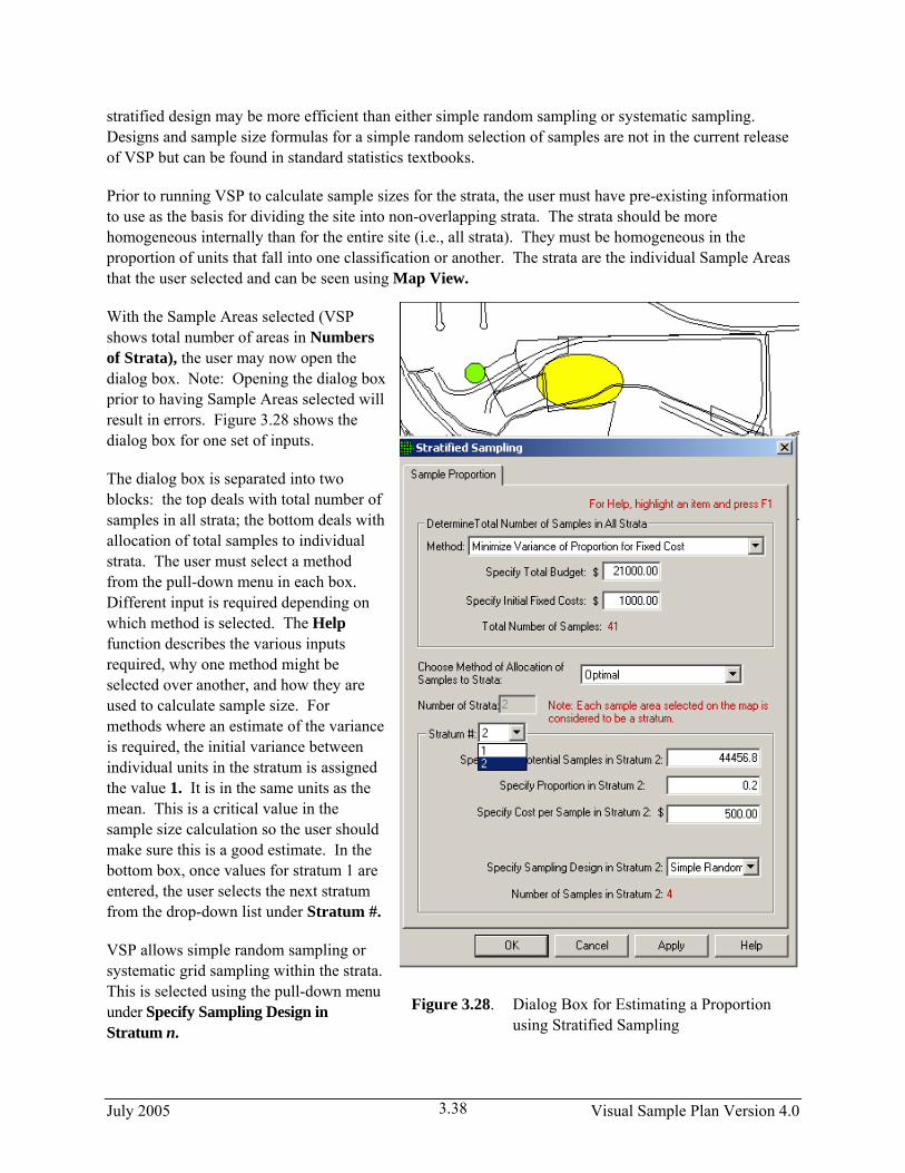
In Figure 3.17, we see the dialog box for entering parameters for stratified sampling. Prior to running VSP to calculate sample sizes for the strata, the user must have pre-existing information to divide the site into non-overlapping strata that are expected to be more homogeneous internally than for the entire site (i.e., all strata). They must be homogeneous in the variable of interest for which we want to calculate a mean. The strata are the individual user-selected Sample Areas and can be seen using Map View.

With the Sample Areas selected (VSP shows total number of areas in Numbers of Strata), the dialog shows the initial values VSP assigns to the various inputs. The number of potential samples in each stratum is initially set at the number of 1-square-foot (or whatever units are used) units available to be sampled or approximately the area of the Sample Area (shown when the area is first selected). If the sample support is not a 1-square-foot volume, the user should change this to the correct value. The initial standard deviation between individual units in the stratum is assigned the value 1. It is in the same units as the mean. This is a critical value in the sample size calculation, so the user should make sure this is a good estimate. The sampling and measurement costs per sample in each stratum and the fixed costs are input in dollars. After entering the values for stratum 1, the user selects the next stratum from the drop-down list under Stratum #.

Figure 3.17. Dialog Box for Stratified Sampling for Estimating a

Mean


VSP allows simple random sampling or systematic within the strata. This is selected using the pull-down menu under Specify Sampling Design in Stratum n.

The other inputs required by VSP pertain to the method the user wants to use for determining 1) the total number or samples in all strata and 2) the allocation of samples to strata. Methods are selected from the drop-down lists. VSP Help offers some insight into why one method might be selected over another, but the user should use the DQO process to flush out the site-specific conditions and project goals that will determine these inputs. Different inputs are required depending on which method is selected for determining the total number of samples. After you press Apply, the dialog shows in red the total number of samples and the number of samples in each stratum (use the pull-down Stratum # to switch between strata). You can see the placement of samples within strata by going to Map View.

3.2.3.2 Ranked Set Sampling

Ranked set sampling (RSS) is the second option for the Sampling Goal: Estimate the Mean > Data not required to be normally distributed. The number of inputs required for RSS is the most of any of the designs available in VSP. However, RSS may offer significant cost savings, making the effort to evaluate the design worthwhile. The VSP Help, the VSP technical report (Gilbert et al. 2002), and EPA (2001, pp. 79–111) are good resources for understanding what is required and how VSP uses the input to create a sampling design.

A simple example given here will explain the various input options. The user should have gone through the DQO process prior to encountering this screen because it provides a basis for inputs.

Under the tab Ranked Set Sampling, the first set of inputs deals with whether this design has any cost advantages over simple random sampling or systematic sampling where every unit that is sampled is measured and analyzed.

We select Symmetric for the distribution of lab data, thus telling VSP we think the lab data is distributed normally so VSP should use a balanced design. A balanced design has the same number of field locations, say r = 4, sampled for each of the say m = 3 ranks. That is, a sample is collected at each of the four locations expected to have a relatively small value of the variable of interest, as well as at the four locations expected to have a mid-range value, and at four locations expected to have a relatively large value. An unbalanced design has more samples collected at locations expected to have large values. EPA says that a balanced design should be used if the underlying distribution of the population is symmetric (EPA 2001, p. 86).

We select Professional Judgment as the ranking method. This selection requires us to say whether we think there is Minimal or Substantial error in our ranking ability. We select Minimal. Note: if we had chosen to use some type of Field Screening device to do the ranking, we would need to provide an estimate of the correlation between the field screening measurements and accurate analytical lab measurements. We choose a set size of 3 from the pull-down menu. The set size we select is based on practical constraints on either our judgment or the field screening equipment available.

Note: VSP uses set size to calculate the factor by which the cost of ranking field locations must be less than lab measurement costs in order to make RSS cost-effective. For our example, VSP tells us this factor must be at least 3 times.


The next set of inputs required for RSS is information required to calculate the number of samples needed for simple random sampling. This value, along with cost information, is used to calculate the number of cycles, r. We say we want a one-sided confidence interval (we want a tight upper bound on the mean and are not concerned about both over- and underestimates of the sample mean), we want that interval to contain 95% of the possible estimates we might make of the sample mean, we want that interval width to be no greater than 1 (in units of how the sample mean is measured), and we estimate the standard deviation between individual units in the population to be 3 (in units of how the sample mean is measured). VSP tells us that if we have these specifications, we would need 26 samples if we were to take them randomly and measure each one in an analytical lab.

The box in the lower right corner of this dialog gives us VSP’s recommendations for our RSS design: we need to rank a total of 45 locations. However, we need to send only 15 of those off to a lab for accurate measurement. This is quite a savings over the 26 required for simple random sampling. There will be r = 5 cycles required.

Note: If we had chosen an unbalanced design, VSP would tell us how many times the top ranked location needed to be sampled per cycle. Also, the inputs for the confidence interval would change slightly for the unbalanced design.

All costs (fixed, field collection per sample, analytical cost for sending a sample to the lab, and ranking cost per location) are entered on the dialog box that appears when the Cost tab is selected. In Figure 3.18, we see the two dialog boxes for RSS.

Once we press Apply, the RSS toolbar appears on our screen. The RSS toolbar lets us explore the locations to be ranked and the locations to be sampled and measured under Map View. VSP produces sample markers on the map that have different shapes and colors. The color of the marker indicates its cycle. The cycle colors start at red and go through the spectrum to violet. Selecting one of the cycles on the pull-down menu displays only the field locations for that cycle. In Figure 3.19, all the green field locations for Cycle 3 are shown. The shape of the marker indicates its set. Field sample locations for the first set are

Figure 3.18. Dialog Boxes for Ranked Set Sampling Design


Figure 3.19. Map of RSS Field Sample Locations for All Sets in Cycle 3, Along with RSS Toolbar

marked with squares, locations for the second set are marked with triangles, and so on. We show All Sets in Figure 3.19. For unbalanced designs, the top set is sampled several times, so a number accompanies those markers. Our example is for a balanced design so we do not see numbers.

Ranked set field sampling locations are generated with a label having the following format: RSS-c-s-i

where c = the cycle number s = the set number (the unbalanced design for this number is also incremented for each iteration of

the top set) I = a unique identifier within the set.

Use View > Labels > Labels on the main menu or the AB button on the mtoolbar (button also on the RSS toolbato show or hide the labels for the field sample locations. Figure 3.20 shows thelabels on the map for field sample locations associated with Cycle 3, All Sets.

ain r)

3.2.3.3 Collaborative Sampling for Estimating the Mean

The third design we discuss for a cost-effective option for estimating the mean when normality cannot be assumed is Collaborative Sampling (CS) – sometimes called Double Sampling. This design is applicable where two or more techniques are available for measuring the amount of pollutant in an environmental sample, for

Figure 3.20. Map of RSS Field Sampling Locations Along with Their Labels


example a field method (inexpensive, less accurate) and a fixed lab method (expensive, more accurate). The approach is to use both techniques on a small number of samples, and supplement this information with a larger of number of samples measured only by the more expensive method. This approach will be cost-effective if the linear correlation between measurements obtained by both techniques on the same samples is sufficiently near 1 and if the less accurate method is substantially less costly than the more accurate method

Collaborative Sampling works like this: At n field locations selected using simple random sampling or grid sampling, the inexpensive analysis method is used. Then, for each of nE of the n locations, the expensive analysis method is also conducted. The data from these two analysis methods are used to estimate the mean and the standard error (SE: the standard deviation of the estimated mean). The method of estimating the mean and SE assumes there is a linear relationship between the inexpensive and expensive analysis methods.

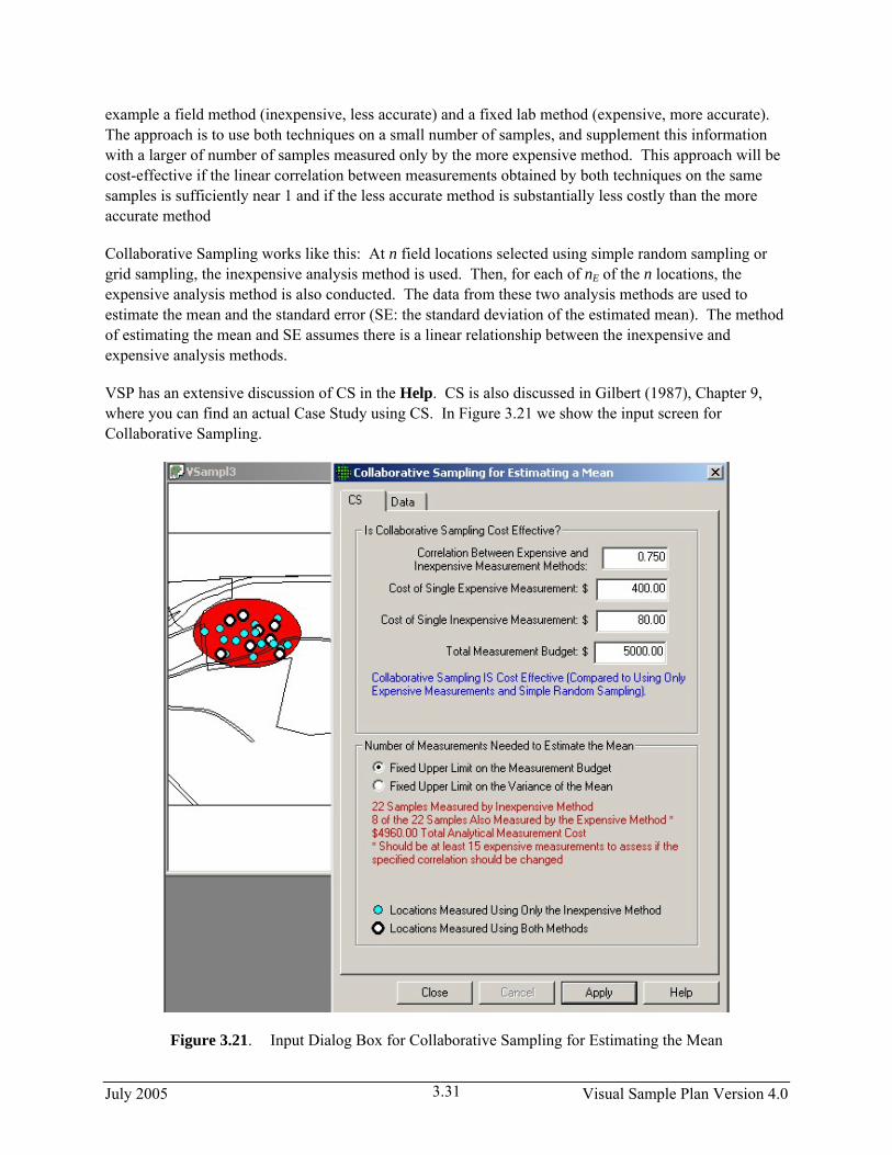
VSP has an extensive discussion of CS in the Help. CS is also discussed in Gilbert (1987), Chapter 9, where you can find an actual Case Study using CS. In Figure 3.21 we show the input screen for Collaborative Sampling.

Figure 3.21. Input Dialog Box for Collaborative Sampling for Estimating the Mean


For this example, we applied CS samples to an area on the Millsite map. After inputting the costs of each measurement technique, the total budget, and an estimate of the correlation between the two methods, VSP informs you whether or not CS is cost effective. For the vales we input, we see that it is cost effective. Then VSP uses the formulas discussed in the On-Line Help and the Report view to calculate two sample sizes, n (22), and nE (8). There are two options for optimizing the values of n and nE that the VSP user must select from:

• estimate the mean with the lowest possible standard error (SE: the standard deviation of the estimated mean) under the restriction that there is a limit on the total budget, or

• estimate the mean under the restriction that the variance of the estimated mean (square of the SE) does not exceed the variance of the mean that would be achieved if the entire budget were devoted to doing only expensive analyses.

We select the first option. VSP calculates that we need to take 22 samples and measure them with the inexpensive method, 8 of which are also measured using the more expensive methods. However, we get a warning message that we should be taking at least 15 measurements where we use both methods in order for VSP to assess whether our initial estimate of a 0.75 linear correlation coefficient is correct. Note that after we hit the Apply button, we see the sampling locations placed on the Sample Area we selected (Millsite.dxf used for this example).

As with Collaborative Sampling for Hypothesis Testing discussed in Section 3.2.1, VSP requires us to input the results of the sampling to verify that the computed correlation coefficient is close to the estimated correlation coefficient used to calculate the sample sizes. Data Results are input in the dialog box that appears after selecting the Data tab (see Figure 3.10b). VSP calculates the estimated mean and standard deviation of the estimated mean once the data values are input.

3.2.3.4 Adaptive Cluster Sampling

Adaptive cluster sampling is appropriate if we can assume the target population is normally distributed: Sampling Goal > Estimate the Mean > Can assume data will be normally distributed > Adaptive Cluster Sampling. Because adaptive designs change as the results of previous sampling become available, adaptive cluster sampling is one of the two VSP designs that require the user to enter sample values while planning a sampling plan. (The other design that requires entering results of previous sampling is sequential sampling; see Section 3.2.1). The VSP Help, the VSP technical report (Gilbert et al. 2002), and the EPA (2001, pp. 105-112) are good resources for understanding what is required and how VSP uses the input to create a sampling design. A simple example here will explain the various input options. The user should have gone through the DQO process prior to encountering this screen because it provides a basis for inputs.

The screen for entering values in the dialog box is displayed by selecting the tab Number of Initial Samples. Adaptive cluster sampling begins by using a probability-based design such as simple random sampling to select an initial set of field units (locations) to sample. To determine this initial sample number, either a one-sided or two-sided confidence interval is selected. We select One-sided Confidence Interval and enter that we want a 95% confidence that the true value of the mean is within this interval. We want an interval width of at least 1 and we estimate the standard deviation between individual units in


the population to be 2 (units of measure for interval width and standard deviation is same as that of individual sample values). VSP returns a value of 13 as the minimum number of initial samples we must take in the Sample Area.

In Figure 3.22, we can see the 13 initial samples as yellow squares on the map.

Figure 3.22. Map of Sample Area with Initial Samples for Adaptive Cluster Sampling Shown as Yellow Squares, Along with Dialog Box

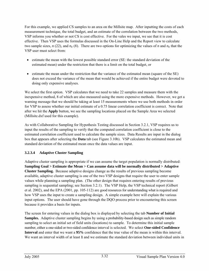
The user now enters the analytical measurement results for the initial 13 sampling units. (Adaptive cluster sampling is most useful when quick turnaround of analytical results is possible, e.g., use of field measurement technology.) Place the mouse directly over each sample and right-click. An input box appears as shown in Figure 3.23. Enter a measurement value (shown here as 8) and, if desired, a label (shown here as AC1-25-62). Press OK. Enter another sample value and continue until all 13 sample values have been entered.

Select tab Grid Size & Follow-Up Samples on the Adaptive Cluster for Estimating a Mean dialog box. Enter the desired Grid Size for Samples, shown here as 20 ft, and an upper threshold measurement value that, if exceeded, triggers additional sampling. We chose 10 as the threshold. We have a choice of how to expand sampling once the threshold is exceeded: 4 nearest neighbors or 8 nearest neighbors. We choose 4. The dialog box is shown as the insert in Figure 3.24a. The grid units can be orientated at different angles by selecting Edit > Sample Areas > Set Grid Angle and Edit > Sample Areas > Reset Grid Angle from the main menu.


Figure 3.23. Dialog Input Box for Entering Sample Measurement Values and Labels for Initial Samples in Adaptive Cluster Sampling

Figure 3.24a. Dialog Input Box for Entering Grid Size and Follow-up Samples


Once Measurement values have been entered, the yellow squares turn to either green, indicating the sample did not exceed the threshold, or red, indicating the sample exceeded the threshold. The red samples are surrounded with additional yellow squares that now must be sampled. This process continues until there are no more yellow grid cells. In Figure 3.24b, we see examples of green, single yellow, red surrounded by yellow, and red surrounded by green. Sampling and measurement continues until all the initial samples are green or red and all the added samples are green or red.

Figure 3.24b. Examples of Combinations of Initial and Follow-up Samples from Adaptive Cluster Sampling

Costs are entered using the Cost tab on the dialog box. The Report for adaptive cluster sampling shows the total cost for all the initial samples plus follow-up samples and provides an (unbiased) estimate of the mean and its standard error. Refer to VSP’s Help for a complete discussion of adaptive cluster sampling.

3.2.4 Construct Confidence Interval on Mean

If the VSP wants a confidence interval on the true value of the mean, not just a point estimate of the mean as calculated in Section 3.2.3, the user selects Sampling Goal > Construct Confidence Interval on the Mean. Currently VSP has algorithms for only the case where the data can assumed to be normally distributed. Within that category, the user can choose Ordinary Sampling or Collaborative Sampling.

For Ordinary Sampling, four DQO inputs are required:

• whether a one- or two-sided interval is desired, • the confidence you want to have that the interval does indeed contain the true value of the mean,


• the maximum acceptable half-width of confidence interval, and • an estimate of the standard deviation between individual units of the population.

The two-sided confidence interval, smaller interval width sizes, and larger variation generally require more samples. In Figure 3.25, we see an example of the design dialog for the Confidence Interval on the Mean sampling goal for Ordinary Sampling, along with the recommended sample size of 38 that VSP calculated.

Figure 3.25. Dialog Input Box for Calculating a Confidence Interval on the Mean using Ordinary Sampling

If the user has more than one type of sample measurement method available, Collaborative Sampling should be explored to see if cost savings are available. Though not shown here, the inputs for Collaborative Sampling for Confidence Interval are similar to those in Figure 3.25, with the added cost inputs required to determine if Collaborative Sampling is cost effective (see discussion of Collaborative Sampling in Section 3.2.3.3). Note that under the sampling goal of Construct Confidence Interval on the Mean, Collaborative Sampling is put under the assumption of “normality”, while for the sampling goal of Estimate the Mean, Collaborative Sampling is put under the assumption of “Data not required to be normally distributed.” This is because for Estimating the Mean, the calculation of sample size n is based on restrictions on the budget or restrictions on the variance which make no distributional assumptions; while for Construct Confidence Interval on the Mean, the calculation of n is based on percentiles of the standard normal distribution.

3.2.5 Compare Proportion to Fixed Threshold

For comparing a proportion to a threshold (i.e., a given proportion), the designs available in VSP do not require the normality assumption. A one-sample proportion test is the basis for calculating sample size. The inputs required to calculate sample size are shown in the design dialog in Figure 3.26. The DQO inputs are similar to those for comparing an average to a fixed threshold, but since the variable of interest is a proportion (percentage of values that meet a certain criterion or fall into a certain class) rather a measurement, the action level is stated as a value from 0.01 to 0.99. Based on the inputs shown in Figure 3.26, VSP calculates that a sample size of 23 is required.


3.2.6 Compare Proportion to Reference Proportion

3.37

Figure 3.26. Design Dialog for Comparing a Proportion to a Fixed Threshold

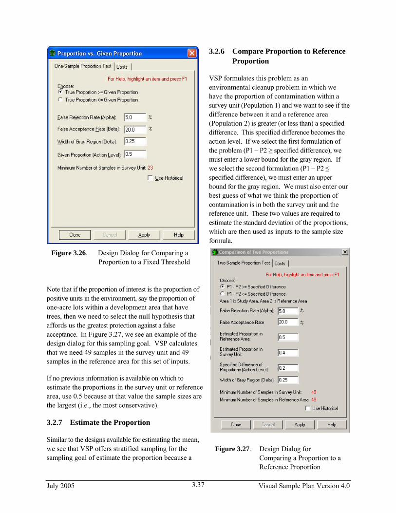
VSP formulates this problem as an environmental cleanup problem in which we have the proportion of contamination within a survey unit (Population 1) and we want to see if tdifference between it and a reference area (Population 2) is greater (or less than) a specified difference. This specified difference becomes the action level. If we select the first formulation of the problem (P1 – P2 ≥ specified difference), we must enter a lower bound for the gray region. If we select the second formulation (P1 – P2 ≤ specified difference), we must enter an upper bound for the gray region. We must also enter our best guess of what we think the proportion of contamination is in both the survey unit and the reference unit. These two values are required to estimate the standard deviation of the proportions, which are then used as inputs to the sample size formula.

he

Note that if the proportion of interest is the proportion of positive units in the environment, say the proportion of one-acre lots within a development area that have trees, then we need to select the null hypothesis that affords us the greatest protection against a false acceptance. In Figure 3.27, we see an example of the design dialog for this sampling goal. VSP calculates that we need 49 samples in the survey unit and 49 samples in the reference area for this set of inputs.

If no previous information is available on which to estimate the proportions in the survey unit or reference area, use 0.5 because at that value the sample sizes are the largest (i.e., the most conservative).

3.2.7 Estimate the Proportion

Similar to the designs available for estimating the mean, we see that VSP offers stratified sampling for the sampling goal of estimate the proportion because a

Figure 3.27. Design Dialog for Comparing a Proportion to a

Reference Proportion

July 2005 Visual Sample Plan Version 4.0

stratified design may be more efficient than either simple random sampling or systematic sampling. Designs and sample size formulas for a simple random selection of samples are not in the current release of VSP but can be found in standard statistics textbooks.

Prior to running VSP to calculate sample sizes for the strata, the user must have pre-existing information to use as the basis for dividing the site into non-overlapping strata. The strata should be more homogeneous internally than for the entire site (i.e., all strata). They must be homogeneous in the proportion of units that fall into one classification or another. The strata are the individual Sample Areas that the user selected and can be seen using Map View.

Figure 3.28. Dialog Box for Estimating a Proportion using Stratified Sampling

With the Sample Areas selected (VSP shows total number of areas in Numbers of Strata), the user may now open the dialog box. Note: Opening the dialog box prior to having Sample Areas selected will result in errors. Figure 3.28 shows the dialog box for one set of inputs.

The dialog box is separated into two blocks: the top deals with total number of samples in all strata; the bottom deals with allocation of total samples to individual strata. The user must select a method from the pull-down menu in each box. Different input is required depending on which method is selected. The Help function describes the various inputs required, why one method might be selected over another, and how they are used to calculate sample size. For methods where an estimate of the variance is required, the initial variance between individual units in the stratum is assigned the value 1. It is in the same units as the mean. This is a critical value in the sample size calculation so the user should make sure this is a good estimate. In the bottom box, once values for stratum 1 are entered, the user selects the next stratum from the drop-down list under Stratum #.

VSP allows simple random sampling or systematic grid sampling within the strata. This is selected using the pull-down menu under Specify Sampling Design in Stratum n.


After supplying the required input, press Apply and the dialog shows in red the total number of samples and the number of samples required in each stratum (use the pull-down Stratum # to switch between strata). You can see the placement of samples within strata by going to Map View.

3.2.8 Locating a Hot Spot

There will be occasions when it is necessary to determine with a specified high probability that no hot spots of a specified size and shape exist in the study area. A hot spot is a local contiguous area that has concentrations that exceed a threshold value. Initially, the conceptual site model should be developed and used to hypothesize where hot spots are most likely to be present. If no hot spots are found by sampling at the most likely locations, then VSP can be used to set up a systematic square, rectangular or triangular sampling grid to search for hot spots. Samples or measurements are made at the nodes of the systematic grid. The VSP user specifies the size and shape of the hot spot of concern, the available funds for collecting and measuring samples, and the desired probability of finding a hot spot of critical size and shape. Either circular or elliptical hot spots can be specified.

The VSP user can direct VSP to compute one or more of the following outputs:

• The number and spacing of samples on the systematic sampling grid that are required to achieve a specified high probability that at least one of the samples will fall on a circular or elliptical hotspot of the specified size.

• The probability that at least one of the samples collected at the nodes of the specified systematic sampling grid will fall on a circular or elliptical hot spot of specified size.

• The probability that at least one of the samples will fall on a hot spot of the specified size given that the spacing between nodes of the systematic sampling grid is the minimum that can be achieved with project funding.

• The smallest size circular or elliptical hot spot that will be detected with specified high probability by sampling at the nodes of the systematic sampling grid.

The basic structure for these problems is that there are four variables (grid spacing, size of hot spot, probability of hitting a hot spot, and cost). You can fix any three of them and solve for the remaining variable.

The other unique feature of the hot spot problem is that there is only one type of error—the false negative or alpha error. VSP asks for only one probability for some formulations of the problem—the limit you want to place on missing a hot spot if it does indeed exist. The other error, saying a hot spot exists when it doesn’t, cannot occur because we assume that if we do get a “hit” at one of the nodes, it is unambiguous (we hit a hot spot). We define hot spots as having a certain fixed size and shape, i.e., no amorphous, contouring hot spots are allowed. The hot spot problem is not a test of a hypothesis. Rather, it is a geometry problem of how likely it is that you could have a hot spot of a certain size and shape fitted within a grid, and none of the nodes fall upon the hot spot.

All the input dialog boxes for of the Hot Spot problem will not be shown in this user’s manual. VPS’s Help, and the textbook Statistical Methods for Environmental Pollution Monitoring (Gilbert 1997) are


good resources for a complete discussion of the Hot Spot problem. We demonstrate a common formulation of the problem—find the minimum number of samples to find a hot spot of a certain size, with specified confidence of hitting the hot spot.

Problem Statement: A site has one Sample Area of one acre (43,560 square feet). We wish to determine the triangular grid spacing necessary to locate a potential circular pocket of contamination with a radius of 15 feet. We desire the probability of detecting such a hot spot, if it exists, to be at least 95%. The fixed planning and validation cost is $1,000. The field collection cost per sample is $50, and the laboratory analytical cost per sample is $100. Assume that the budget will be provided to support the sampling design determined from these requirements.

Case 9: We assume that the assumptions listed in Gilbert (1987, p. 119) are valid for our problem. We specify a hit probability of 95%, a shape of 1.0 (circular), and a radius (Length of Semi-Major Axis) of 15 feet. We will let VSP calculate the length of the side of the equilateral triangular grid needed for these inputs.

VSP Solution 9: First, open the file OneAcre.vsp using VSP Main Menu option File > Open Project. This is a VSP-formatted project file and it contains a previously defined Sample Area of the entire acre. Next, from the VSP Main Menu select Sampling Goals > Locating a Hot Spot > Systematic Grid. A grouping of the input dialogs for the four tabs: Locating Hot Spot, Grid, Hot Spot, and Costs are shown in Figure 3.29.

Figure 3.29. Input Boxes for Case 9 for Locating a Hot Spot


Figure 3.29. (contd)

The recommended length of grid side is shown in the dialog box for Locating a Hot Spot, Solve for Grid Spacing. It is about 28.98 feet or, rounding up, a 30-foot triangular grid.

Note: For this set of inputs, VSP will always give the length of the triangular grid as 28.98 feet. The Calculated total number of samples in the Report View is always 60 for this set of inputs. However, the Number of samples on the map changes as you repeatedly press the Apply button. This occurs whenever the Random Start check box in the dialog box tabbed Find Grid is checked. Because the starting point of the grid is random, the way in which the grid will fit inside the Study Area can change with each new random-start location. More or fewer sampling locations will occur with the same grid size, depending on how the sampling locations fall with respect to the Sample Area’s outside edges.

The input dialog boxes and report for the hot spot problem have some unique features:

• Placing the cursor in the Length of Semi-Major Axis on the Hot Spot tab and right-clicking displays a black line on the picture of the circle for the radius.

• Shape controls how “circular” the hot spot is. Smaller values (0.2) result in a more elliptical shape; 1.0 is a perfect circle.

• The user can specify the Area of the hot spot or the Length of the Semi-Major Axis. Both fields have pull-down menus for selecting the unit of measurement.

• The Report provides additional information on the design such as the number of samples (both “on the map” and “calculated”) and grid area.


The Hot Spot Sampling Goal takes into account the Total Area to Sample (see this field on the Cost tab) when calculating total number of samples. Many of the other designs use the standard deviation to control sample size.

3.2.9 Find UXO Target Areas

The next two Sampling Goals originated from specific unexploded ordinance (UXO) problems faced by the Department of Defense. The sampling designs the VSP developers came up with to address these problems are somewhat specialized. A separate User’s Manual is available for the UXO Modules (Version 2.0 Visual Sample Plan: UXO Module Code Description and Verification, PNNL -14267, Gilbert et al., 2003) which can be downloaded from the VSP web site: http://dqo.pnl.gov/VSP. We present in this User’s Manual a brief summary of the UXO designs.

At military ranges used for target practice, UXO could be expected to lie within a circular or elliptical “target area” of debris where ordnance missed the exact target and explosions scattered debris objects. The goal is to find these “target areas” by conducting geophysical surveys along transects (swaths) and detecting areas where metallic or explosive debris objects are more densely located than is expected in the (non target area) background. The swath width is the width of the geophysical sensor or sensor arrays; the spacing between swaths is calculated to achieve a specified level of confidence of finding circular or elliptical target areas. The problem separates into three distinct Sampling Goals:

• Find a swath spacing design that will locate elliptical or circular target areas

• In a post-survey situation, find the probability that a given set of transects will indeed transect and detect a target area of a specified size and shape

• Find areas of elevated anomaly densities in a set of pre-loaded swaths with anomalies placed on top of the swaths

Again, we point the user to the extensive VSP On-Line Help for these Sampling Goals, and the PNNL report referenced above for details not included in the brief discussion below.

3.2.9.1 Find Swath Spacing

The VSP menu selection Sampling Goals > Find UXO Target Areas > Parallel or Grid Sampling… brings up the dialog box shown in Figure 3.30. There are two parts to the problem: not only must the geophysical detector traverse (pass over) the target area (this is similar to the Hot Spot problem), it must also detect that a target area has been traversed (this is a simple false negative detection problem). Inputs for addressing these two parts to the problem are shown in the top and bottom boxes in Figure 3.30. In the top box, the desired probability of traversing the target, the swath pattern desired, and swath width of the detector are specified. VSP calculates the swath spacing required to detect the target defined under the Target Zone tab. In this example, VSP calculates a swath spacing of 23.33 ft is required, assuming a circular target of 10 ft radius, and a 10 ft swath width—making the swath spacing 23.33 + 10 = 33.33 ft on centers.

In the bottom part of the dialog box, labeled Target Detection, the user inputs information about the density of objects or UXO expected within the target area and the false negative detection rate of the


http://dqo.pnl.gov/VSP

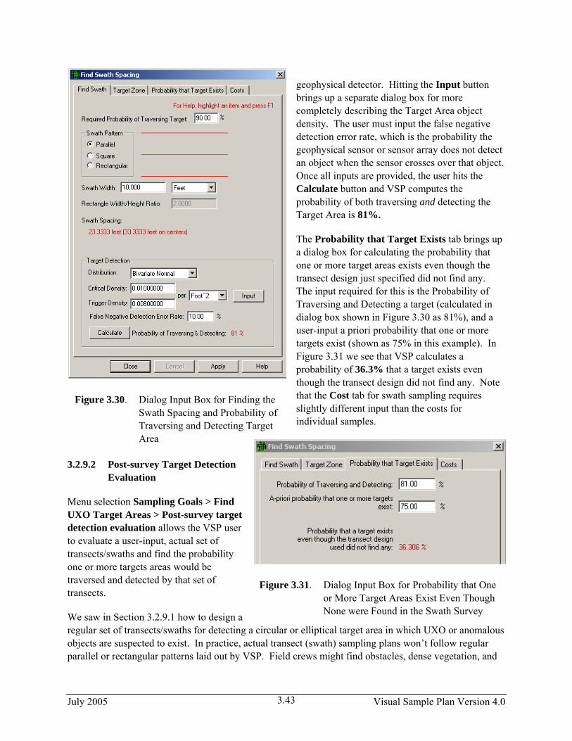
geophysical detector. Hitting the Input button brings up a separate dialog box for more completely describing the Target Area object density. The user must input the false negative detection error rate, which is the probability the geophysical sensor or sensor array does not detect an object when the sensor crosses over that object. Once all inputs are provided, the user hits the Calculate button and VSP computes the probability of both traversing and detecting the Target Area is 81%.

The Probability that Target Exists tab brings up a dialog box for calculating the probability that one or more target areas exists even though the transect design just specified did not find any. The input required for this is the Probability of Traversing and Detecting a target (calculated in dialog box shown in Figure 3.30 as 81%), and a user-input a priori probability that one or more targets exist (shown as 75% in this example). In Figure 3.31 we see that VSP calculates a probability of 36.3% that a target exists even though the transect design did not find any. Note that the Cost tab for swath sampling requires slightly different input than the costs for individual samples.

3.2.9.2 Post-survey Target Detection Evaluation

Menu selection Sampling Goals > Find UXO Target Areas > Post-survey target detection evaluation allows the VSP user to evaluate a user-input, actual set of transects/swaths and find the probability one or more targets areas would be traversed and detected by that set of transects.

We saw in Section 3.2.9.1 how to design a regular set of transects/swaths for detecting a circular or elliptical target area in which UXO or anomalous objects are suspected to exist. In practice, actual transect (swath) sampling plans won’t follow regular parallel or rectangular patterns laid out by VSP. Field crews might find obstacles, dense vegetation, and

Figure 3.30. Dialog Input Box for Finding the Swath Spacing and Probability of Traversing and Detecting Target Area

Figure 3.31. Dialog Input Box for Probability that One or More Target Areas Exist Even Though None were Found in the Swath Survey


other factors making it impossible to follow straight lines. To address this, VSP allows the user to input a set of “meandering swaths” (Map > Meandering Swaths), and then through simulation, calculates the probability of traversing, and traversing and detecting a user-specified Target Zone/Area. Figure 3.32a shows a Map View of a user-input meandering swath. Figure 3.32b shows a meandering swath with width reflecting the width of the detection equipment as it traverses the ground. The Help function describes this feature in more detail. Meandering swaths are loaded only if they fall inside a Selected Sample Area.

Figure 3.32a. Imported Meandering S(series of connected lines)

wath Figure 3.32b. Imported Meandering Swath with width (series of connected rectangles)

Menu selection Sampling Goals > Find UXO Target Areas > Post-survey target detection evaluation brings up the dialog box for inputting the information VSP needs to perform a simulation of the performance of a given set of transects/swaths. The dialog box is shown in Figure 3.33. Swath must be imported or created within a Sample Area before running the simulations.

The Detection Simulation tab has inputs required for the two simulations: Target Traversal, and Target Detection. The user selects the number of trials for the simulation, shown here as 10,000. When the Target Transversal “Simulate” button is pushed, VSP throws down the 10,000 trial target areas and counts the number that touch one of the swath segments. A “hit” occurs when a trial target area touches a swath segment. The Probability of Traversing is computed as the number of hits divided by the number of trial targets, computed as 89% for this example.

The inputs for the Target Detection are similar to those required for Find Swath Spacing (Section 3.2.9.1). When the Target Detection “Simulate” button is pushed, VSP throws down the number of trial target areas and determines the probability that each target area will be traversed and detected, making use of the critical density of anomalies in the target area, the trigger density at which the user is concerned about finding, and the false negative error rate of the sensor for actually detecting anomalies. For the inputs shown, this probability is 49%.


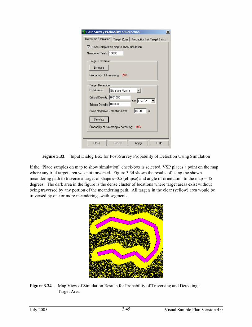
Figure 3.33. Input Dialog Box for Post-Survey Probability of Detection Using Simulation

If the “Place samples on map to show simulation” check-box is selected, VSP places a point on the map where any trial target area was not traversed. Figure 3.34 shows the results of using the shown meandering path to traverse a target of shape s=0.5 (ellipse) and angle of orientation to the map = 45 degrees. The dark area in the figure is the dense cluster of locations where target areas exist without being traversed by any portion of the meandering path. All targets in the clear (yellow) area would be traversed by one or more meandering swath segments.

Figure 3.34. Map View of Simulation Results for Probability of Traversing and Detecting a Target Area


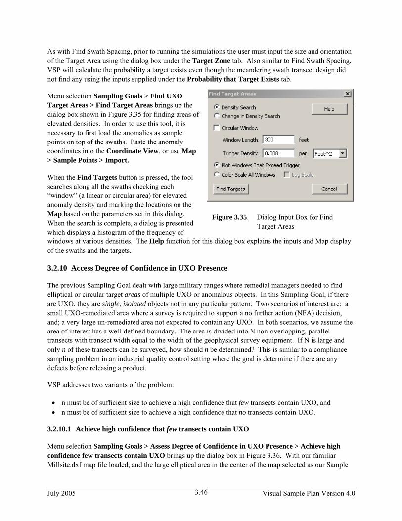
As with Find Swath Spacing, prior to running the simulations the user must input the size and orientation of the Target Area using the dialog box under the Target Zone tab. Also similar to Find Swath Spacing, VSP will calculate the probability a target exists even though the meandering swath transect design did not find any using the inputs supplied under the Probability that Target Exists tab.

Menu selection Sampling Goals > Find UXO Target Areas > Find Target Areas brings up the dialog box shown in Figure 3.35 for finding areas of elevated densities. In order to use this tool, it is necessary to first load the anomalies as sample points on top of the swaths. Paste the anomaly coordinates into the Coordinate View, or use Map > Sample Points > Import.

Figure 3.35. Dialog Input Box for Find Target Areas

When the Find Targets button is pressed, the tool searches along all the swaths checking each “window” (a linear or circular area) for elevated anomaly density and marking the locations on the Map based on the parameters set in this dialog. When the search is complete, a dialog is presented which displays a histogram of the frequency of windows at various densities. The Help function for this dialog box explains the inputs and Map display of the swaths and the targets.

3.2.10 Access Degree of Confidence in UXO Presence

The previous Sampling Goal dealt with large military ranges where remedial managers needed to find elliptical or circular target areas of multiple UXO or anomalous objects. In this Sampling Goal, if there are UXO, they are single, isolated objects not in any particular pattern. Two scenarios of interest are: a small UXO-remediated area where a survey is required to support a no further action (NFA) decision, and; a very large un-remediated area not expected to contain any UXO. In both scenarios, we assume the area of interest has a well-defined boundary. The area is divided into N non-overlapping, parallel transects with transect width equal to the width of the geophysical survey equipment. If N is large and only n of these transects can be surveyed, how should n be determined? This is similar to a compliance sampling problem in an industrial quality control setting where the goal is determine if there are any defects before releasing a product.

VSP addresses two variants of the problem:

• n must be of sufficient size to achieve a high confidence that few transects contain UXO, and • n must be of sufficient size to achieve a high confidence that no transects contain UXO.

3.2.10.1 Achieve high confidence that few transects contain UXO

Menu selection Sampling Goals > Assess Degree of Confidence in UXO Presence > Achieve high confidence few transects contain UXO brings up the dialog box in Figure 3.36. With our familiar Millsite.dxf map file loaded, and the large elliptical area in the center of the map selected as our Sample


Area, we input a transect width of 10 ft. VSP informs us that there are N= 64 total non-overlapping transects within this Sample Area. The 64 transects are shown in yellow in Figure 3.36. The VSP user inputs 10% as an upper limit on the maximum allowed percent of transects that could contain one or more UXO (DQO input), and 90% as the confidence that this maximum percent is not exceeded.

VSP calculates that 20 of the 64 transects must be selected, using simple random sampling, and none of these transects can contain UXO in order to be “90% confident that less than 10% of all possible transects contain UXO”. The n=20 randomly selected transects that VSP placed on the Map when the Apply button is pushed are shown in pink in Figure 3.36. The algorithm for calculating sample size n programmed into VSP for this problem is a method developed by E.G. Schilling called “compliance sampling”. For extensive discussion of this problem and compliance sampling methods consult VSP’s Help and Gilbert, et al (The Schilling and Wright/Grieve Methods for Assessing Compliance with USO Requirements, 2003), or Gilbert, et al. (Version 2.0 Visual Sample Plan (VSP): UXO Module Code Description and Verification, PNNL-14267, 2003; Chapter 6).

Figure 3.36. Dialog Input Box for Compliance Sampling for UXO and Map of Sample Area with Transects Selected


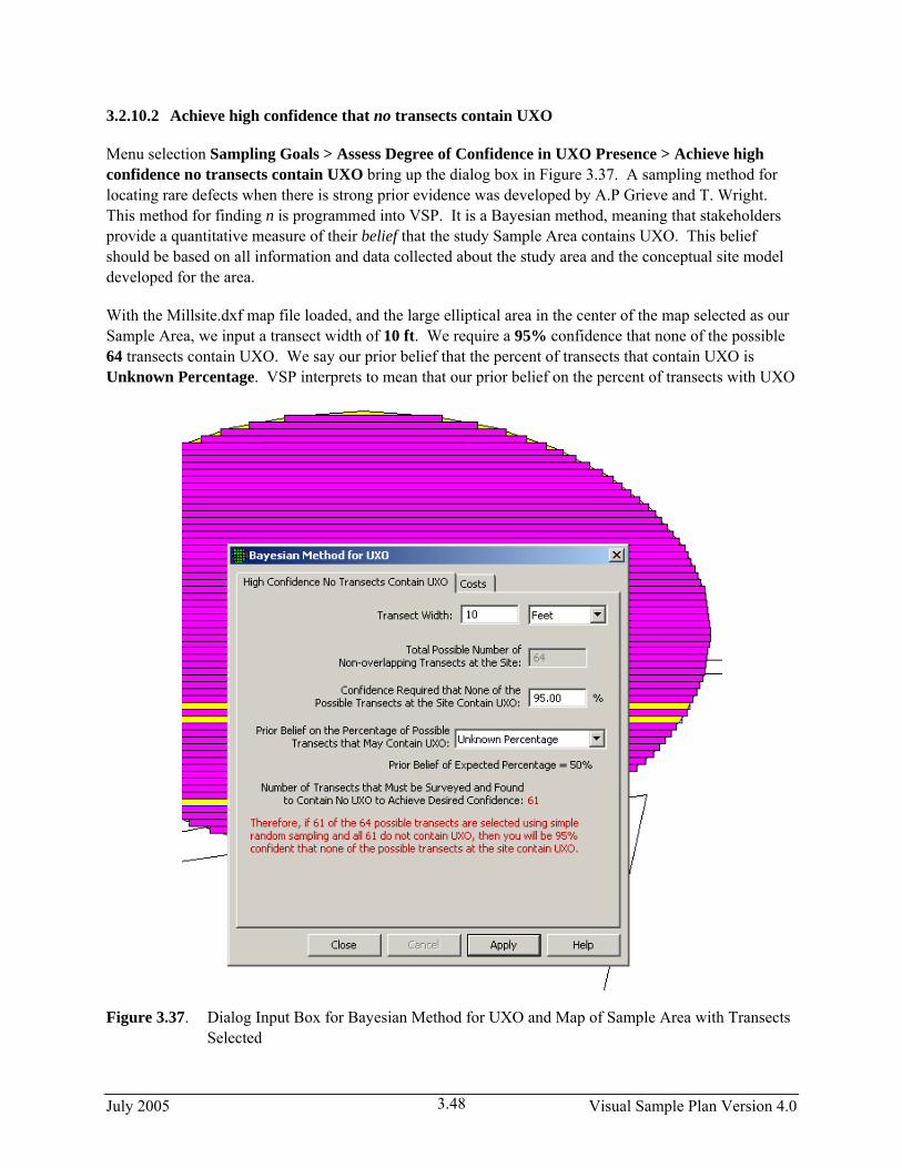
3.2.10.2 Achieve high confidence that no transects contain UXO

Menu selection Sampling Goals > Assess Degree of Confidence in UXO Presence > Achieve high confidence no transects contain UXO bring up the dialog box in Figure 3.37. A sampling method for locating rare defects when there is strong prior evidence was developed by A.P Grieve and T. Wright. This method for finding n is programmed into VSP. It is a Bayesian method, meaning that stakeholders provide a quantitative measure of their belief that the study Sample Area contains UXO. This belief should be based on all information and data collected about the study area and the conceptual site model developed for the area.

With the Millsite.dxf map file loaded, and the large elliptical area in the center of the map selected as our Sample Area, we input a transect width of 10 ft. We require a 95% confidence that none of the possible 64 transects contain UXO. We say our prior belief that the percent of transects that contain UXO is Unknown Percentage. VSP interprets to mean that our prior belief on the percent of transects with UXO

Figure 3.37. Dialog Input Box for Bayesian Method for UXO and Map of Sample Area with Transects Selected


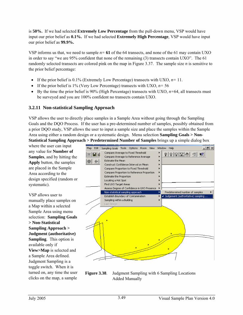
is 50%. If we had selected Extremely Low Percentage from the pull-down menu, VSP would have input our prior belief as 0.1%. If we had selected Extremely High Percentage, VSP would have input our prior belief as 99.9%.

VSP informs us that, we need to sample n= 61 of the 64 transects, and none of the 61 may contain UXO in order to say “we are 95% confident that none of the remaining (3) transects contain UXO”. The 61 randomly selected transects are colored pink on the map in Figure 3.37. The sample size n is sensitive to the prior belief percentage:

• If the prior belief is 0.1% (Extremely Low Percentage) transects with UXO, n= 11. • If the prior belief is 1% (Very Low Percentage) transects with UXO, n= 56 • By the time the prior belief is 90% (High Percentage) transects with UXO, n=64, all transects must

be surveyed and you are 100% confident no transects contain UXO.

3.2.11 Non-statistical Sampling Approach

VSP allows the user to directly place samples in a Sample Area without going through the Sampling Goals and the DQO Process. If the user has a pre-determined number of samples, possibly obtained from a prior DQO study, VSP allows the user to input a sample size and place the samples within the Sample Area using either a random design or a systematic design. Menu selection Sampling Goals > Non-Statistical Sampling Approach > Predetermined Number of Samples brings up a simple dialog box where the user can input any value for Number of Samples, and by hitting the Apply button, the samples are placed in the Sample Area according to the design specified (random or systematic).

Figure 3.38. Judgment Sampling with 6 Sampling Locations Added Manually

VSP allows user to manually place samples on a Map within a selected Sample Area using menu selection: Sampling Goals > Non-Statistical Sampling Approach > Judgment (authoritative) Sampling. This option is available only if View>Map is selected and a Sample Area defined. Judgment Sampling is a toggle switch. When it is turned on, any time the user clicks on the map, a sample


marker is placed at that location. Judgment samples can be added to a blank Map or to an existing design. The Type is “Manual” (see View > Coordinates). Manual samples may also be added by typing the coordinates (x, y) on the keyboard.

In Figure 3.39, 6 samples have manually been added using Judgment Sampling.

3.2.12 Establish Boundary of Contamination

Finding the boundary of contamination is a problem faced by Department of Defense remediation managers. Training ranges or aother contaminants of concern) may have boundaries that completely or partially enclose the contaminated area. Sampling is required to determine whether contamination has breached a known boundary line and if so, determine the correct boundary line. VSP has a special module for this samplinproblem. The problem and the VSP solution are described in Visual Sample Plan User’s Guide for Establishing the Boundary of Contamination, R.O. Gilbert, et al, PNWD-3580, 2005, which can be downloaded from the VSP web site

reas

g

Figure 3.39. Judgment Sampling with Six Sampling Locations Added Manually

where the soil is known to contain explosive residues (or

http://dqo.pnl.gov/VSP. In this User’s Guide wsummary description of the VSP boundary module.

e will provide a

The VSP sampling design for this problem involves taking a representative sample (called a multiple

In Sections 2.3.1.1 and 2.3.1.2 we described how to define enclosing and partial boundaries in VSP using

ced

r-

VSP provides two versions of the design: one for enclosing boundaries and one for partial (open-type)

type

increment or MI) for each segment along the known, user-input boundary. If the one or more samplesshow contamination, extend or “bump out” the boundary, and take more samples. The boundary continues to be bumped out until all samples taken along the new boundary line are “clean”.

Edit >Sample Areas > Define New Sample Area, and Edit > Sample Areas > Define New Open-Type Sample Area, respectively. VSP determines the number of segments using the length of the boundary and the specified width of a contaminant plume (hot spot) that would be of concern if it is present at the boundary or extends beyond the boundary line. VSP calculates the optimum segment length (OSL) alongthe current boundary, where all segments have the same length. One or two MI samples are collected per segment. VSP assumes that each MI sample collected in a segment consists of 25 small soil samples (increments) that have been collected in sets of 5 small samples clustered around each of 5 equally spaPrimary Sampling Locations along the segment. The spacing of the five segments depends on the specified width of the hot spot of concern at the boundary. The OLS is calculated as 5 times the usespecified width of the contamination plume (hot spot) of concern.

boundaries. Partial boundaries represent a dividing line, with contamination on one side and no contamination on the other side. VSP provides special tools for creating and manipulating open-sample areas.



3.2.12.1 Enclosing Boundary

Menu selection Sampling Goals > Establish Boundary of Contamination > Enclosing Boundary brings up the dialog box in Figure 3.40 for tab Enclosed Boundary Sampling. The first input required is the confidence needed that the mean calculated from limited sample data is indeed less than the action limit. For this example, that confidence level is 95%. The diameter of the area of contamination (i.e., the hot spot) that the user wants to be sure is detected at the boundary is input as 45 ft. The next box, labeled Duplicate Requirements, has to do with how many of the segments need duplicate MI samples to be collected. VSP requires that: at least 5 segments; or at least 10% of the segments, need duplicates. The user may select which requirement is used. While 10% is the minimum, the user may input any percentage for duplicates.

Figure 3.40. Dialog Box for Entering Design Inputs for Sampling an Enclosing Boundary Note: The purpose of duplicate MI

samples is to estimate the relative standard deviation of the data so that an Upper Confidence Limit (UCL) test can be conducted for each segment. See VSP Help for more information.

If the boundary of the site is very irregular, e.g., has various indentations, the VSP user can specify in the dialogue box that VSP should change the boundary to a convex hull. This has the effect of smoothing

out the boundary irregularities, but it also enlarges the area enclosed by the initial boundary. In practice, the VSP user can try this option and view the resulting initial boundary to see if the new boundary is acceptable. In Figure 3.40 we leave this box unchecked.

The user now must input the contaminates of concern and the threshold (action level) at which we want VSP to trigger extending the contamination boundary line. The dialog box for tab Analytes is shown in Figure 3.41. VSP provides a default list of contaminants of concern (TNT, RDX, and HMX) and a default list of upper limit values (Action Limit) for each (16ppm, 4.4ppm, and 3100ppm). To

Figure 3.41. List of Default Contaminants of Concern and their Action Levels


remove a contaminant from the list, erase the name and the limit. To add a contaminant, enter its name and threshold value in the blank lint below the last contaminant.

For the Millsite.dxf map file selected, and the central ellipse in the center of the map selected as the Sample Area with an enclosing boundary, we see in Figure 3.42 that after clicking the Apply button in the previous screen, VSP divides the boundary into 12 segments. Shown are the 5 equally-spaced Primary Sampling Locations in each of the segments. The segments for which the Primary Sample Locations are in bold type will have duplicate samples taken at each location. Different symbols are assigned to each segment to differentiate the segments visually. For each segment, VSP assumes the user will form the MI sample for that segment by mixing 5 small soil samples collected from each of the 5 Primary Sampling Locations. Hence, each MI sample is formed from the 25 small soil samples.

Figure 3.42. An Enclosing Boundary Showing the Five Primary Sampling Locations for Each of the 17 Segments

The user now collects the samples, mixes the samples to form a representative MI sample for each segment, and measures each MI sample. The results are input into VSP using the Sample Information box that appears when the cursor is placed over one of the Primary Sample Locations, and right-click the mouse. Use the keyboard to enter the measurement value into the appropriate row in the column labeled “Value” in the Segment Sample Results sub-box. Use the down arrow button on the keyboard to move between rows within the sub-box. Figure 3.43 shows the Sample Information Box.

We happened to click on a segment for which two MI samples are required. Thus, we will need to input two sets of measurements, one for each of the 3 analytes, making 6 input values required. Click the OK button on the dialog box to close the Sample Information box for that segment. Repeat the above process for each of the segments to enter all the measurement values. The Segment Sample Results box has a column headed “UCL”. VSP will fill in this box with the Upper Confidence Limit on the mean once all the measurement values for the segment are input. The UCL is used to test whether the mean exceeds the action level for that segment.

Sample results can be entered into VSP using software such as a spreadsheet. Consult VSP’s Help for instructions on this process.


Figure 3.43. Sample Information Box for Entering Data into VSP, Duplicate Samples Required

VSP now tests whether each boundary segment should be enlarged (bumped out). This is described in an Appendix to the report PNWD-3580 referenced above. In Figure 3.44 we see an example of two expanded boundaries. Note the red colored Primary Location Segments indicate that segment did not pass the UCL test and hence had to be “bumped out”.

Figure 3.44. Enclosed Boundary with Two Bumped-Out Segments


3.2.12.2 Partial Boundaries

The input screens, the dialog boxes, and the maps for Partial Boundaries problems are similar to those for the Enclosed Boundaries and will not be shown here. For a discussion of the Partial Boundaries problem consult the VSP Help function.

3.2.13 Sampling Within Buildings

While many of the sampling designs presented in earlier sections could be applied to 3-dimensional sample areas such as building and rooms (-- as opposed to 2-dimensional sample areas such as land areas), the sampling designs provided under Sampling within a Building are uniquely suited for problems where contamination is released into an enclosed structure and contamination can be on walls and ceilings, windows and doors, as well as on floors. Many of the VSP features added for this module were requested by the Department of Homeland Security (DHS), Combating Terrorism Technology Support Office. DHS wanted ways to sample walls, floors, ceilings, and other surfaces to determine if contamination is present, its magnitude and extent throughout the building, and after decontamination to see if the decon was effective. The sub-goals within this section work through various scenarios when a chemical, biological or radionuclide release has occurred within a building, and contamination may be: isolated; microscopic; pose a health risk at very low levels of contamination; selectively adheres to surfaces and crevices; capable of being spread throughout the building; and generally from an unknown source and released in an unknown location within the building. The unique nature of these contamination scenarios requires unique sampling methods and unique analysis methods.

Figure 3.45 is a schematic of the menu options available under the sampling goal of Sampling within a Building.

In the case of a terrorist bio/chem/rad event, the parameters of interest will most likely be the mean, maximum, or a percentile of the distribution of all possible measurements. So the first major branch in the menu tree is whether a decision on contamination will be made based on the mean/average, on

Unknown distribution ...

No sample exceedancespermitted ...

Collaborative sampling ...

Ordinary sampling - No distributional assumption (MARSSIM) ...

Upper tolerance limit

Acceptance sampling

Can assume data will be normally distributed

Data not required to be normally distributed

Detect hotspots ...

Ensure no contamination ...

Compare average to threshold

Compare measurements to threshold

Combined Average and Individual Measurement Criteria ...

Sampling within a Building Ensure most of area is uncontaminated

Ordinary sampling of symmetric distribution ...

Ordinary sampling ...

Sequential sampling (Known Std Dev) ...

Sequential sampling (Unknown Std Dev) ...

Normally distributed ...

Some sample exceedancespermitted ...

Unknown distribution ...

No sample exceedancespermitted ...

Collaborative sampling ...

Ordinary sampling - No distributional assumption (MARSSIM) ...

Upper tolerance limit

Acceptance sampling

Can assume data will be normally distributed

Data not required to be normally distributed

Detect hotspots ...

Ensure no contamination ...

Compare average to threshold

Compare measurements to threshold

Combined Average and Individual Measurement Criteria ...

Sampling within a Building Ensure most of area is uncontaminated

Ordinary sampling of symmetric distribution ...

Ordinary sampling ...

Sequential sampling (Known Std Dev) ...

Sequential sampling (Unknown Std Dev) ...

Normally distributed ...

Some sample exceedancespermitted ...

Figure 3.45. Menu Structure of Options Under Sampling Goal of Sampling Within a Building


individual measurements, or on a combination of both. Depending on which branch is selected, very different menu options will be offered, very different sampling designs will be suggested, and very different comparisons and analyses will be performed.

In the sections below, we will provide a brief discussion of each of the end points (i.e., VSP-recommended sampling designs) for the menu tree in Figure 3.45. Some of the designs in the tree have been recommended for other sampling goals in VSP and have been discussed in earlier sections of this manual. Consequently, in this part of the manual we will focus the discussion on the designs that are unique to Sampling within a Building. For selected designs (Figs 3.46b and 3.48b), we show the samples located within simple rooms that we drew in VSP so the user can see how VSP places samples (both point samples and grid samples) on the floor, ceiling, walls, windows and doors of a room.

Several papers and presentations have been published on the designs and analyses associated with Sampling within a Building. In addition to the technical discussions found in the VSP online Help for each design, consult the VSP web page (http://dqo.pnl.gov/VSP) for papers and presentations on the theory behind the designs and data analyses. A complete technical discussion and verification of all tests, sample size calculations, and algorithms used in Sampling within Buildings can be found in Technical Documentation and Verification for the Buildings Module in the Visual Sample Plan (VSP) Software, Gilbert et al., PNNL-15202, available for download on the VSP web page.

3.2.13.1 Compare Average to a Threshold

A threat analysis team would be interested in average contamination within a building or room if there were multiple releases and subsequent spread of contamination, and the primary exposure scenario concerned an accumulated dose, or a long-term exposure of individuals randomly moving about within the room/building. The sampling goal would be to take samples and compare the average contamination in a room, or a group of rooms, to a health risk-based threshold.

A number of statistical sampling designs could be applicable depending on the assumptions, constraints, and sampling technologies. These designs include simple random sampling, grid sampling, sequential sampling, and collaborative sampling. Similarly, a number of tests could be conducted on the data to decide if the mean is greater than a threshold. These tests include the one-sample t test, a sign test, or a ranked sum test. All the designs within this sampling goal have been discussed earlier in the manual under the sampling goal of Compare Average to Fixed Threshold (Section 3.2.1).

3.2.13.2 Compare Individual Measurements to a Threshold

Most biological, chemical, or radiological threats involve a risk to an individual if any exposure to the contaminant is encountered. As such, there is an interest in individual (rather than average) measurements. If the entire area/decision unit cannot be surveyed, the goal may be to take limited samples and based on those samples, make statements (with the associated confidence level) about unsampled areas. Another goal might be to make a confidence statement about the percent of the total population that is contaminated, based on sample data. For each goal, one of the VSP outputs is a statement that can be made based on sample results. For example, for the sampling goal Sampling within a building > Compare measurements to threshold > Ensure most of the area uncontaminated > Acceptance Sampling > No sample exceedances permitted, after providing the



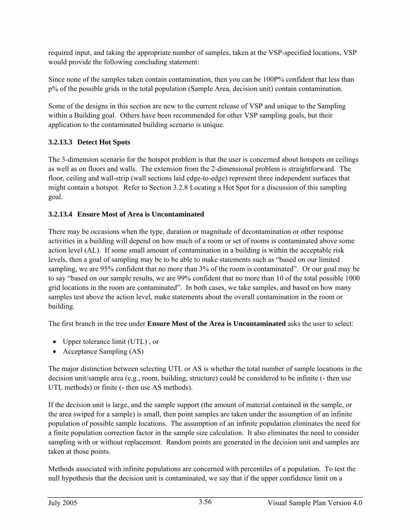
required input, and taking the appropriate number of samples, taken at the VSP-specified locations, VSP would provide the following concluding statement:

Since none of the samples taken contain contamination, then you can be 100P% confident that less than p% of the possible grids in the total population (Sample Area, decision unit) contain contamination.

Some of the designs in this section are new to the current release of VSP and unique to the Sampling within a Building goal. Others have been recommended for other VSP sampling goals, but their application to the contaminated building scenario is unique.

3.2.13.3 Detect Hot Spots

The 3-dimension scenario for the hotspot problem is that the user is concerned about hotspots on ceilings as well as on floors and walls. The extension from the 2-dimensional problem is straightforward. The floor, ceiling and wall-strip (wall sections laid edge-to-edge) represent three independent surfaces that might contain a hotspot. Refer to Section 3.2.8 Locating a Hot Spot for a discussion of this sampling goal.

3.2.13.4 Ensure Most of Area is Uncontaminated

There may be occasions when the type, duration or magnitude of decontamination or other response activities in a building will depend on how much of a room or set of rooms is contaminated above some action level (AL). If some small amount of contamination in a building is within the acceptable risk levels, then a goal of sampling may be to be able to make statements such as “based on our limited sampling, we are 95% confident that no more than 3% of the room is contaminated”. Or our goal may be to say “based on our sample results, we are 99% confident that no more than 10 of the total possible 1000 grid locations in the room are contaminated”. In both cases, we take samples, and based on how many samples test above the action level, make statements about the overall contamination in the room or building.

The first branch in the tree under Ensure Most of the Area is Uncontaminated asks the user to select:

• Upper tolerance limit (UTL) , or • Acceptance Sampling (AS)

The major distinction between selecting UTL or AS is whether the total number of sample locations in the decision unit/sample area (e.g., room, building, structure) could be considered to be infinite (- then use UTL methods) or finite (- then use AS methods).

If the decision unit is large, and the sample support (the amount of material contained in the sample, or the area swiped for a sample) is small, then point samples are taken under the assumption of an infinite population of possible sample locations. The assumption of an infinite population eliminates the need for a finite population correction factor in the sample size calculation. It also eliminates the need to consider sampling with or without replacement. Random points are generated in the decision unit and samples are taken at those points.

Methods associated with infinite populations are concerned with percentiles of a population. To test the null hypothesis that the decision unit is contaminated, we say that if the upper confidence limit on a


percentile of the population is less than the limit, then we can reject the null hypothesis and conclude the decision unit is uncontaminated. A confidence interval on a percentile of a population is called a tolerance interval. The tests in this group calculate an Upper tolerance limit (UTL) for the population and compare it to a limit. The UTL is calculated from sample results. The methods of Upper tolerance limit are used for infinite populations.

If the decision unit (i.e., a room) is small relative to the sample support, and the sample support is well-defined (say the sample will consist of a 4 inch square swab), then samples are taken under the assumption of a finite population of all possible sample locations. We would partition the room into individual, non-over-lapping “grid” locations, specify the total number of grids in the room, specify the number of grids to be sampled, then use a random selection of size n (calculated by VSP) grids to be included in the sample.

Methods associated with finite populations use the concept of “lots”, i.e., a discrete group of units extracted from a total production run. This has application to a decision unit that can be gridded, with each grid unit having a discrete identity within the larger population. The methods of Acceptance sampling (taken from industrial quality control) are used for finite populations. The tests in this group of methods count the number of grids in the sample that exceed an action level (are defective) and as long as that number is less than or equal to an “Acceptance Number”, we say the level of contamination is within the tolerable (i.e., acceptable) limits.

Ensure most of the area is uncontaminated > Upper tolerance

limit > Normally distributed

If the distribution of measurements of contamination at all possible point sample locations in the decision unit can be considered to be normally distributed (i.e., the standard bell-shaped curve), we can use the formula that calculates the UTL of a percentile of the normal distribution in the test of the null hypothesis. This UTL will be compared to the Action Level to determine whether we accept or reject the null hypothesis. The UTL formula will also be used in the calculation of the sample size, n. Figure 3.46a shows the dialog box for this sampling goal.

The null hypothesis being tested is that the true Pth percentile of the population exceeds a fixed Action Level (i.e., the

Figure 3.46a. Dialog Input Box for Comparing Percentile of Normal Distribution to Action Level


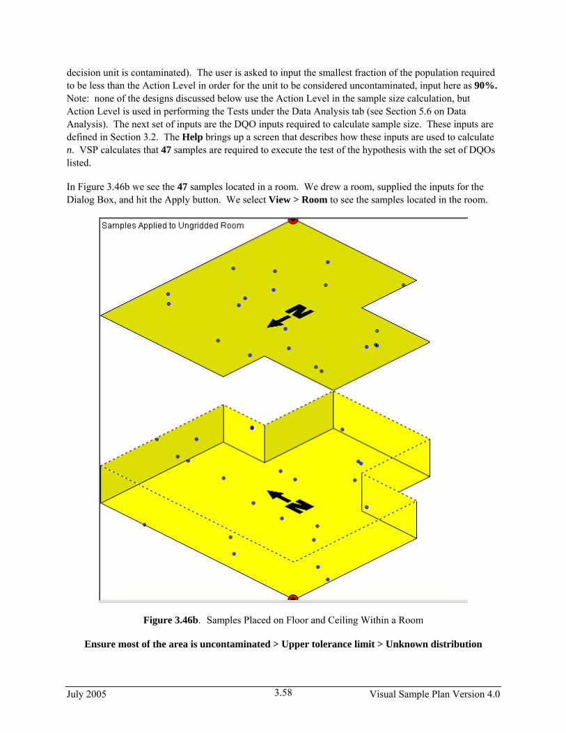
decision unit is contaminated). The user is asked to input the smallest fraction of the population required to be less than the Action Level in order for the unit to be considered uncontaminated, input here as 90%. Note: none of the designs discussed below use the Action Level in the sample size calculation, but Action Level is used in performing the Tests under the Data Analysis tab (see Section 5.6 on Data Analysis). The next set of inputs are the DQO inputs required to calculate sample size. These inputs are defined in Section 3.2. The Help brings up a screen that describes how these inputs are used to calculate n. VSP calculates that 47 samples are required to execute the test of the hypothesis with the set of DQOs listed.

In Figure 3.46b we see the 47 samples located in a room. We drew a room, supplied the inputs for the Dialog Box, and hit the Apply button. We select View > Room to see the samples located in the room.

Figure 3.46b. Samples Placed on Floor and Ceiling Within a Room

Ensure most of the area is uncontaminated > Upper tolerance limit > Unknown distribution


If the distribution of measurements is unknown, we must calculate a non-parametric UTL for use in the test of the hypothesis that the true Pth percentile of the population exceeds a fixed Action Level. The non-parametric UTL happens to be the largest measurement of the n samples taken, where n is calculated using the DQO inputs in Figure 3.47 and the sample size formula discussed in the VSP Help for this input screen.

VSP calculates that we need to take 29 samples in order to make a 95% confidence statement about the 90th percentile of non-parametric distribution. The exact wording of the conclusion that can be drawn is one of the outputs of VSP. An example conclusion is shown in red in Figure 3.47.

Ensure most of the area is uncontaminated > Acceptance

sampling > No sample exceedances permitted

Figure 3.47. Dialog Input Box for Comparing Percentile of Unknown Distribution to Action Level

If the VSP user’s goal is to specify a proportion defective (called Pd in the Help) which is the maximum tolerable proportion of defective (contaminated above the Action Level) grid units allowed in the population, and wants a high confidence in recognizing when that proportion is exceeded, then this sampling goal is selected. The tab for this sampling goal states that the user wants a “high confidence that few grids contain contamination”. Again taken from quality control literature, the method VSP uses to calculate sample size is called “Compliance Sampling” or “Acceptance Sampling for C = 0”. For this design, the Acceptance Number, C, which is the number of measured grid units in the sample that can exceed the Action Level (i.e., allowed to be defective) is zero. As shown in the Dialog Box in Figure 3.48a, for the user inputs of Action Level = 10, total number of possible grids in the decision unit or room(s) = 1,000, the maximum allowed % of grids in the decision unit that can contain contamination = 10%, and the confidence required that the maximum % is not exceeded = 90%. VSP calculates a sample size of n=24. VSP sets the Total Possible Number of Grids in Selected Rooms to 1000 when no Sample Area/Rooms have been selected. Users can input values of their own choosing for Total Number of Grids when designing sampling plans for items.

A scenario when Compliance Sampling may be applicable is that it is initially assumed that no contamination exists and the goal is to have a high confidence of detecting whether a specified Pd percent of the units in the decision unit are actually contamination.


Shown in red in the Dialog Box, VSP reminds the user that for this design, none of the 24 grids may exceed the Action Level in order to be 90% confident that less than 10% of the population of all grids at the site contain contamination (i.e., above the action level).

Once a room or rooms have been drawn and selected, VSP shows the Length of Grid Side in the Dialog Box and calculates a Total Possible Number of Grids for the Sample Area/Rooms based on that grid size. Note: VSP initially calculates a default value for the Length of Grid Size. The user replaces the default value with a grid length that is appropriate for the type of sample that will be taken, e.g., a 1ft x 1ft square swath, a 4cm x 4cm swab. Hitting the Apply button on the Dialog Box places grids on the selected rooms, and calculates a new Total Possible Number of Grids based on this new grid size.

Figure 3.48a. Dialog Input Box for Compliance Sampling In Figure 3.48b we see an example of a 1ft

x 1ft grid applied to a room that has two closed windows (so samples can be placed on them) and an open door (so samples cannot be placed on it). VSP calculates that 7,284 possible grids of 1ft x 1ft could be placed in the selected room, 24 of which will have samples collected from them. Refer to Section 6.3 on types of objects that can be placed within rooms for an explanation of windows and doors within rooms.

Ensure most of area is uncontaminated > Acceptance sampling > Some sample exceedances permitted

For this sampling goal, the user specifies two proportions: Po, the maximum acceptable proportion of units in the population that are allowed to be contaminated above the Action Level; and Pa, the unacceptable proportion of units in the population that are contaminated above the Action Level. If the number of grid units in the sample that have contamination greater than the Action Level exceeds the Acceptance Number, C (which VSP calculates), then the user concludes the maximum acceptable % of grids contamination has been exceeded and the real proportion defective is equal to or greater than Pa. The method used for this design is called “Acceptance Sampling for C > 0”, or just “Acceptance Sampling”. Note that this method is slightly different from the previously discussed method of Compliance Sampling. Compliance Sampling made a confidence statement about the proportion defective, Pd. Acceptance Sampling is a test of hypothesis between two different statements about the


Figure 3.48b. Room with Samples Placed on Floor, Ceiling, Walls, and Windows

number of defective units in the population, Do and Da (Da > Do). Therefore, Acceptance Sampling for C > 0, requires both an Alpha and a Beta (see Section 3.2). Refer to the Help for a more complete discussion of the method.

A scenario when Acceptance Sampling for C > 0 may be applicable is that you know some level of contamination may exist (naturally occurring, or the level of contamination is at the detection level of the monitoring equipment) to give a lower bound Po. There is an upper bound Pa where a health risk may occur and you want to be have a high confidence of detecting contaminating greater than Pa percent.

The Dialog Input Box for this sampling goal is shown in Figure 3.49. We are asked to input the total number of grid units in the population, shown here as 1,000. Next we input the Action Level and the DQO inputs needed to calculate sample size and the Acceptance Number, C. The acceptable % of grids


Hathaway, John (J)

I don’t see the grid on figure 3.48b.

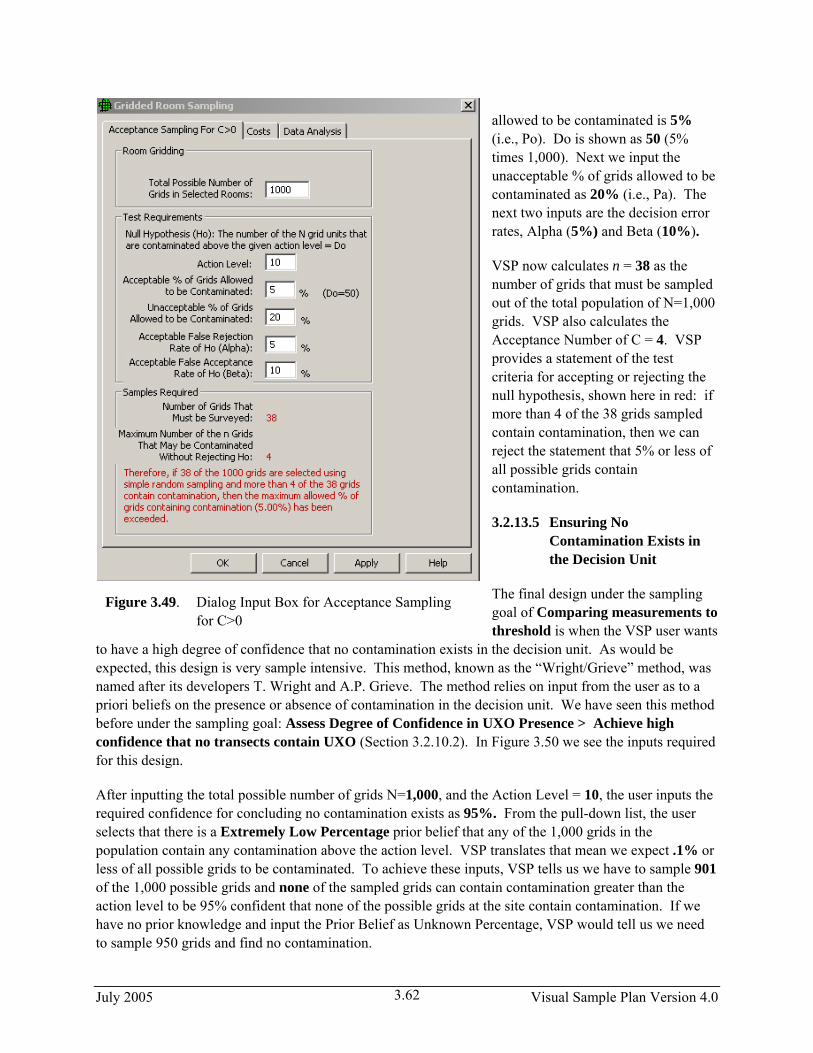
allowed to be contaminated is 5% (i.e., Po). Do is shown as 50 (5% times 1,000). Next we input the unacceptable % of grids allowed to be contaminated as 20% (i.e., Pa). The next two inputs are the decision error rates, Alpha (5%) and Beta (10%).

VSP now calculates n = 38 as the number of grids that must be sampled out of the total population of N=1,000 grids. VSP also calculates the Acceptance Number of C = 4. VSP provides a statement of the test criteria for accepting or rejecting the null hypothesis, shown here in red: if more than 4 of the 38 grids sampled contain contamination, then we can reject the statement that 5% or less of all possible grids contain contamination.

3.2.13.5 Ensuring No Contamination Exists in the Decision Unit

Figure 3.49. Dialog Input Box for Acceptance Sampling for C>0

The final design under the sampling goal of Comparing measurements to threshold is when the VSP user wants

to have a high degree of confidence that no contamination exists in the decision unit. As would be expected, this design is very sample intensive. This method, known as the “Wright/Grieve” method, was named after its developers T. Wright and A.P. Grieve. The method relies on input from the user as to a priori beliefs on the presence or absence of contamination in the decision unit. We have seen this method before under the sampling goal: Assess Degree of Confidence in UXO Presence > Achieve high confidence that no transects contain UXO (Section 3.2.10.2). In Figure 3.50 we see the inputs required for this design.

After inputting the total possible number of grids N=1,000, and the Action Level = 10, the user inputs the required confidence for concluding no contamination exists as 95%. From the pull-down list, the user selects that there is a Extremely Low Percentage prior belief that any of the 1,000 grids in the population contain any contamination above the action level. VSP translates that mean we expect .1% or less of all possible grids to be contaminated. To achieve these inputs, VSP tells us we have to sample 901 of the 1,000 possible grids and none of the sampled grids can contain contamination greater than the action level to be 95% confident that none of the possible grids at the site contain contamination. If we have no prior knowledge and input the Prior Belief as Unknown Percentage, VSP would tell us we need to sample 950 grids and find no contamination.


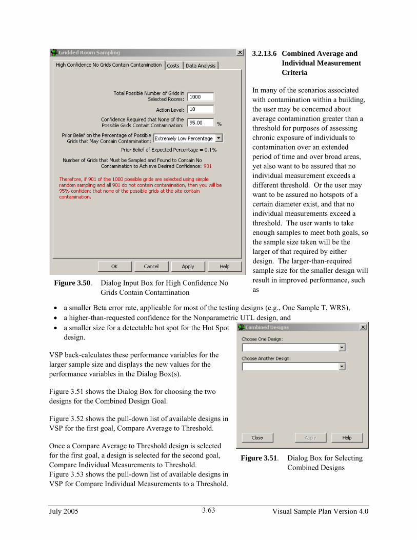
3.2.13.6 Combined Average and Individual Measurement Criteria

In many of the scenarios associated with contamination within a building, the user may be concerned about average contamination greater than a threshold for purposes of assessing chronic exposure of individuals to contamination over an extended period of time and over broad areas, yet also want to be assured that no individual measurement exceeds a different threshold. Or the user may want to be assured no hotspots of a certain diameter exist, and that no individual measurements exceed a threshold. The user wants to take enough samples to meet both goals, so the sample size taken will be the larger of that required by either design. The larger-than-required sample size for the smaller design will result in improved performance, such as

Figure 3.50. Dialog Input Box for High Confidence No Grids Contain Contamination

• a smaller Beta error rate, applicable for most of the testing designs (e.g., One Sample T, WRS), • a higher-than-requested confidence for the Nonparametric UTL design, and • a smaller size for a detectable hot spot for the Hot Spot

design.

VSP back-calculates these performance variables for the larger sample size and displays the new values for the performance variables in the Dialog Box(s).

Figure 3.51 shows the Dialog Box for choosing the two designs for the Combined Design Goal.

Figure 3.52 shows the pull-down list of available designs in VSP for the first goal, Compare Average to Threshold.

Once a Compare Average to Threshold design is selected for the first goal, a design is selected for the second goal, Compare Individual Measurements to Threshold. Figure 3.53 shows the pull-down list of available designs in VSP for Compare Individual Measurements to a Threshold.

Figure 3.51. Dialog Box for Selecting Combined Designs


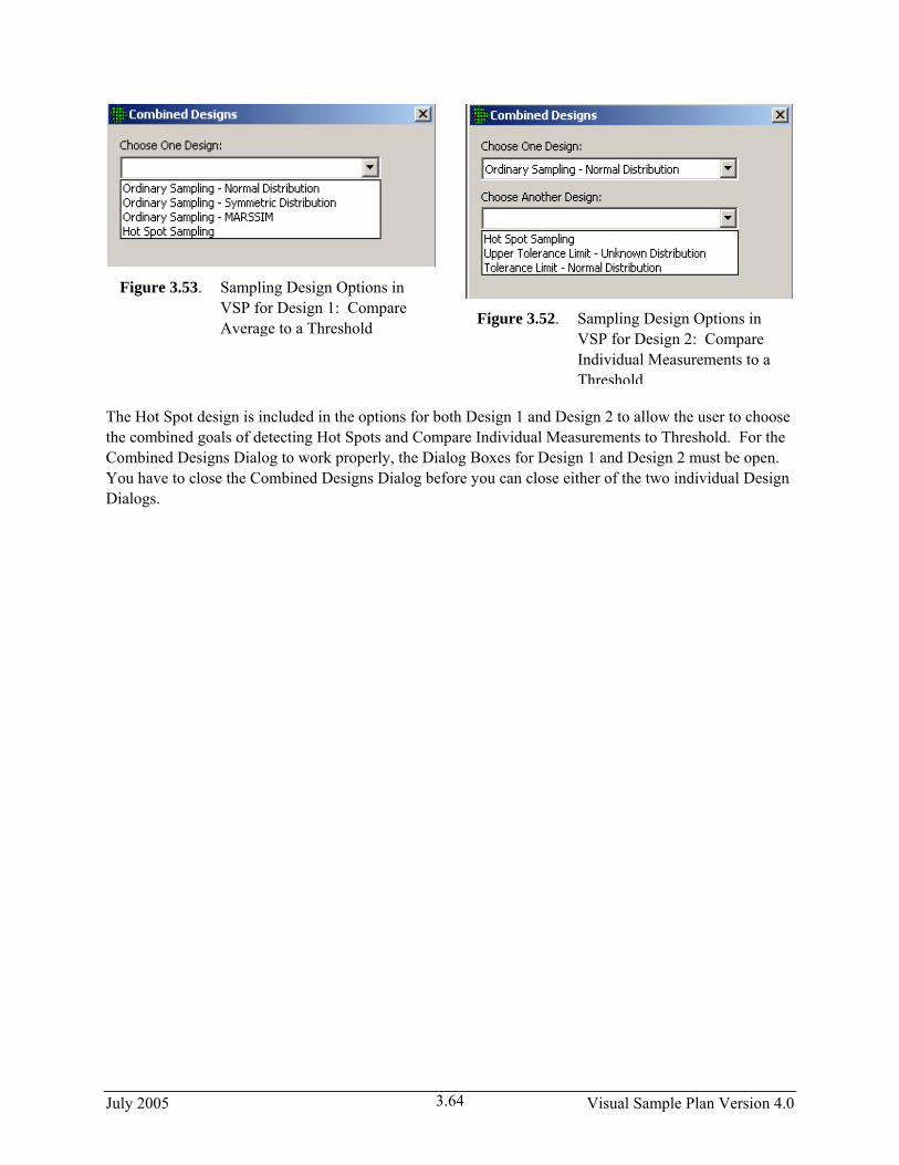
Figure 3.52. Sampling Design Options in VSP for Design 2: Compare Individual Measurements to a Threshold

Figure 3.53. Sampling Design Options in VSP for Design 1: Compare Average to a Threshold

The Hot Spot design is included in the options for both Design 1 and Design 2 to allow the user to choose the combined goals of detecting Hot Spots and Compare Individual Measurements to Threshold. For the Combined Designs Dialog to work properly, the Dialog Boxes for Design 1 and Design 2 must be open. You have to close the Combined Designs Dialog before you can close either of the two individual Design Dialogs.


Documents

3.0 Sampling Plan Development Within VSP · 3.0 Sampling Plan Development Within VSP ... toward a complete set of sampling design ... according to some characteristic or feature of