Embed Size (px)
Citation preview
BS and MI
Xiao-Li Meng
Bootstrap
Replications
MultipleImputation
BayesJustification
Non-BayesianJustification
Self-efficiency
Characterizationsof Self-efficiency
ThreeScenarios
History
30 Years of Bootstrap and Multiple Imputation:Joint Replications vs Conditional Replications
Xiao-Li Meng
Department of Statistics, Harvard University
Thanks to Zhan Li and Xianchao Xie
Supplementing Efron (1994, JASA) & Discussion by Rubin
“Missing Data, Imputation, and the Bootstrap.”
Continuing Meng (1994, Statistical Science)
“Multiple-imputation Inferences With Uncongenial Sources ofInput”

BS and MI
Xiao-Li Meng
Bootstrap
Replications
MultipleImputation
BayesJustification
Non-BayesianJustification
Self-efficiency
Characterizationsof Self-efficiency
ThreeScenarios
History
Celebrating 30+ Years of Bootstrap (Efron, 1977,1979)
IEEE SIGNAL PROCESSING MAGAZINE [10] JULY 2007 1053-5888/07/$25.00©2007IEEE
[A tutorial for the signal processing practitioner]
This year marks the pearl anniversary of the bootstrap. It has been 30 years sinceBradley Efron’s 1977 Reitz lecture, published two years later in [1]. Today, bootstraptechniques are available as standard tools in several statistical software packages andare used to solve problems in a wide range of applications. There have also been sev-eral monographs written on the topic, such as [2], and several tutorial papers writ-
ten for a nonstatistical readership, including two for signal processing practitioners publishedin this magazine [4], [5].
Given the wealth of literature on the topic supported by solutions to practical problems, wewould expect the bootstrap to be an off-the-shelf tool for signal processing problems as are max-imum likelihood and least-squares methods. This is not the case, and we wonder why a signalprocessing practitioner would not resort to the bootstrap for inferential problems.
We may attribute the situation to some confusion when the engineer attempts to discoverthe bootstrap paradigm in an overwhelming body of statistical literature. To give an exampleand ignoring the two basic approaches of the bootstrap, i.e., the parametric and the nonpara-metric bootstrap [2], there is not only one bootstrap. Many variants of it exist, such as the smallbootstrap [6], the wild bootstrap [7], the naïve bootstrap (a name often given to the standardbootstrap resampling technique), the block (or moving block) bootstrap (see the chapter by Liuand Singh in [8]) and its extended circular block bootstrap version (see the chapter by Politisand Romano in [8]), and the iterated bootstrap [9]. Then there are derivatives such as theweighted bootstrap or the threshold bootstrap and some more recently introduced methodssuch as bootstrap bagging and bumping. Clearly, this wide spectrum of bootstrap variants maybe a hurdle for newcomers to this area.
[Abdelhak M. Zoubir and D. Robert Iskander]
BootstrapMethods and Applications
PROF. DR. KARL HEINRICH HOFMANN
BS and MI
Xiao-Li Meng
Bootstrap
Replications
MultipleImputation
BayesJustification
Non-BayesianJustification
Self-efficiency
Characterizationsof Self-efficiency
ThreeScenarios
History
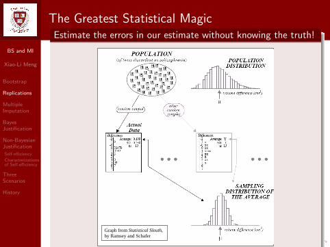
The Greatest Statistical Magic
Estimate the errors in our estimate without knowing the truth!
Graph from Statistical Sleuth, by Ramsey and Schafer
BS and MI
Xiao-Li Meng
Bootstrap
Replications
MultipleImputation
BayesJustification
Non-BayesianJustification
Self-efficiency
Characterizationsof Self-efficiency
ThreeScenarios
History
The Greatest Statistical MagicEstimate the errors in our estimate without knowing the truth!
Graph from Statistical Sleuth, by Ramsey and Schafer
BS and MI
Xiao-Li Meng
Bootstrap
Replications
MultipleImputation
BayesJustification
Non-BayesianJustification
Self-efficiency
Characterizationsof Self-efficiency
ThreeScenarios
History
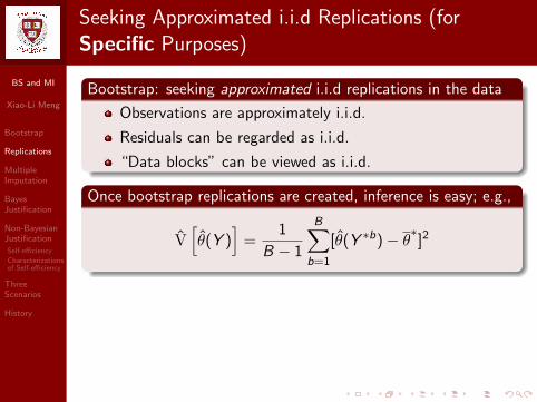
Seeking Approximated i.i.d Replications (forSpecific Purposes)
Bootstrap: seeking approximated i.i.d replications in the data
Observations are approximately i.i.d.
Residuals can be regarded as i.i.d.
“Data blocks” can be viewed as i.i.d.
Once bootstrap replications are created, inference is easy; e.g.,
V[θ(Y )
]=
1
B − 1
B∑b=1
[θ(Y ∗b)− θ∗]2
Multiple Imputation (MI): seeking i.i.d replications of themissing data conditioning on the observed data
MIs are created from posterior predictive sampling:
Y(1)mis , . . . ,Y
(m)mis
i.i.d.∼ PM(Ymis |Yobs)
BS and MI
Xiao-Li Meng
Bootstrap
Replications
MultipleImputation
BayesJustification
Non-BayesianJustification
Self-efficiency
Characterizationsof Self-efficiency
ThreeScenarios
History
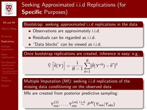
Seeking Approximated i.i.d Replications (forSpecific Purposes)
Bootstrap: seeking approximated i.i.d replications in the data
Observations are approximately i.i.d.
Residuals can be regarded as i.i.d.
“Data blocks” can be viewed as i.i.d.
Once bootstrap replications are created, inference is easy; e.g.,
V[θ(Y )
]=
1
B − 1
B∑b=1
[θ(Y ∗b)− θ∗]2
Multiple Imputation (MI): seeking i.i.d replications of themissing data conditioning on the observed data
MIs are created from posterior predictive sampling:
Y(1)mis , . . . ,Y
(m)mis
i.i.d.∼ PM(Ymis |Yobs)
BS and MI
Xiao-Li Meng
Bootstrap
Replications
MultipleImputation
BayesJustification
Non-BayesianJustification
Self-efficiency
Characterizationsof Self-efficiency
ThreeScenarios
History
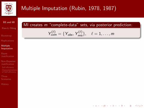
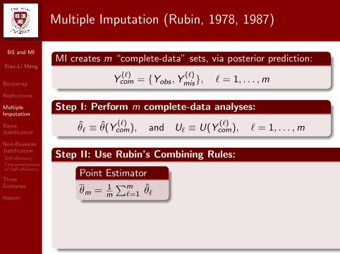
Multiple Imputation (Rubin, 1978, 1987)
MI creates m “complete-data” sets, via posterior prediction:
Y(`)com = {Yobs ,Y
(`)mis}, ` = 1, . . . ,m
Step I: Perform m complete-data analyses:
θ` ≡ θ(Y(`)com), and U` ≡ U(Y
(`)com), ` = 1, . . . ,m
Step II: Use Rubin’s Combining Rules:
Point Estimator
θm = 1m
∑m`=1 θ`
Variance Estimator
Tm = Um +(1 + 1
m
)Bm
Within-Imputation Var
Um = 1m
∑m`=1 U`
Between-Imputation Var
Bm = 1m−1
∑m`=1 (θ`−θm)(θ`−θm)>
BS and MI
Xiao-Li Meng
Bootstrap
Replications
MultipleImputation
BayesJustification
Non-BayesianJustification
Self-efficiency
Characterizationsof Self-efficiency
ThreeScenarios
History
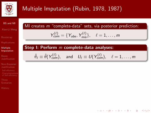
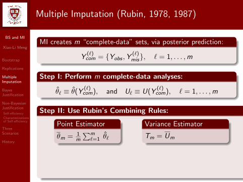
Multiple Imputation (Rubin, 1978, 1987)
MI creates m “complete-data” sets, via posterior prediction:
Y(`)com = {Yobs ,Y
(`)mis}, ` = 1, . . . ,m
Step I: Perform m complete-data analyses:
θ` ≡ θ(Y(`)com), and U` ≡ U(Y
(`)com), ` = 1, . . . ,m
Step II: Use Rubin’s Combining Rules:
Point Estimator
θm = 1m
∑m`=1 θ`
Variance Estimator
Tm = Um +(1 + 1
m
)Bm
Within-Imputation Var
Um = 1m
∑m`=1 U`
Between-Imputation Var
Bm = 1m−1
∑m`=1 (θ`−θm)(θ`−θm)>
BS and MI
Xiao-Li Meng
Bootstrap
Replications
MultipleImputation
BayesJustification
Non-BayesianJustification
Self-efficiency
Characterizationsof Self-efficiency
ThreeScenarios
History
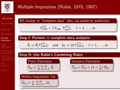
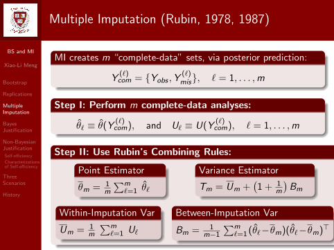
Multiple Imputation (Rubin, 1978, 1987)
MI creates m “complete-data” sets, via posterior prediction:
Y(`)com = {Yobs ,Y
(`)mis}, ` = 1, . . . ,m
Step I: Perform m complete-data analyses:
θ` ≡ θ(Y(`)com), and U` ≡ U(Y
(`)com), ` = 1, . . . ,m
Step II: Use Rubin’s Combining Rules:
Point Estimator
θm = 1m
∑m`=1 θ`
Variance Estimator
Tm = Um
+(1 + 1
m
)Bm
Within-Imputation Var
Um = 1m
∑m`=1 U`
Between-Imputation Var
Bm = 1m−1
∑m`=1 (θ`−θm)(θ`−θm)>

BS and MI
Xiao-Li Meng
Bootstrap
Replications
MultipleImputation
BayesJustification
Non-BayesianJustification
Self-efficiency
Characterizationsof Self-efficiency
ThreeScenarios
History
Multiple Imputation (Rubin, 1978, 1987)
MI creates m “complete-data” sets, via posterior prediction:
Y(`)com = {Yobs ,Y
(`)mis}, ` = 1, . . . ,m
Step I: Perform m complete-data analyses:
θ` ≡ θ(Y(`)com), and U` ≡ U(Y
(`)com), ` = 1, . . . ,m
Step II: Use Rubin’s Combining Rules:
Point Estimator
θm = 1m
∑m`=1 θ`
Variance Estimator
Tm = Um +(1 + 1
m
)Bm
Within-Imputation Var
Um = 1m
∑m`=1 U`
Between-Imputation Var
Bm = 1m−1
∑m`=1 (θ`−θm)(θ`−θm)>
BS and MI
Xiao-Li Meng
Bootstrap
Replications
MultipleImputation
BayesJustification
Non-BayesianJustification
Self-efficiency
Characterizationsof Self-efficiency
ThreeScenarios
History
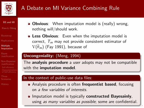
A Debate on MI Variance Combining Rule
Obvious: When imputation model is (really) wrong,nothing will/should work.
Less Obvious: Even when the imputation model iscorrect, Tm may not provide consistent estimator ofV(θm) (Fay 1991), because of
Uncongeniality: (Meng, 1994)
The analysis procedure a user adopts may not be compatiblewith the imputation model.
In the context of public-use data files:
Analysis procedure is often frequentist based, focusingon a few variables of interests.
Imputation model is typically constructed Bayesainly,using as many variables as possible; some are confidential.
BS and MI
Xiao-Li Meng
Bootstrap
Replications
MultipleImputation
BayesJustification
Non-BayesianJustification
Self-efficiency
Characterizationsof Self-efficiency
ThreeScenarios
History
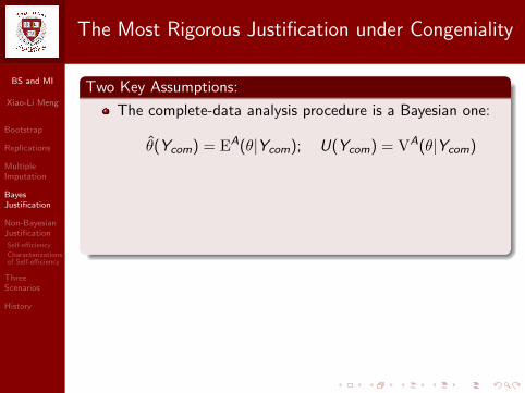
The Most Rigorous Justification under Congeniality
Two Key Assumptions:
The complete-data analysis procedure is a Bayesian one:
θ(Ycom) = EA(θ|Ycom); U(Ycom) = VA(θ|Ycom)
The imputer’s model and analysis model are congenial:
PM(Ymis |Yobs) = PA(Ymis |Yobs), ∀ Ymis
Then for θm as m→∞
θ∞ = EM[θ(Ycom)
∣∣Yobs
]= EM
[EA(θ|Ycom)
∣∣Yobs
]= EA
[EA(θ|Ycom)
∣∣Yobs
]= EA(θ|Yobs)

BS and MI
Xiao-Li Meng
Bootstrap
Replications
MultipleImputation
BayesJustification
Non-BayesianJustification
Self-efficiency
Characterizationsof Self-efficiency
ThreeScenarios
History
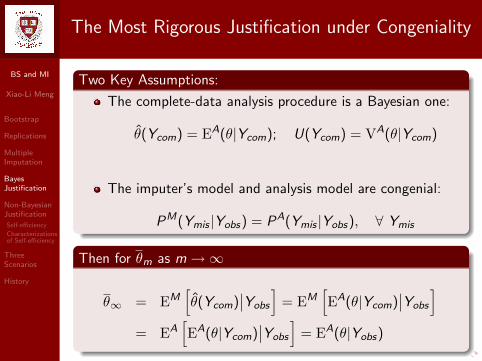
The Most Rigorous Justification under Congeniality
Two Key Assumptions:
The complete-data analysis procedure is a Bayesian one:
θ(Ycom) = EA(θ|Ycom); U(Ycom) = VA(θ|Ycom)
The imputer’s model and analysis model are congenial:
PM(Ymis |Yobs) = PA(Ymis |Yobs), ∀ Ymis
Then for θm as m→∞
θ∞ = EM[θ(Ycom)
∣∣Yobs
]= EM
[EA(θ|Ycom)
∣∣Yobs
]
= EA[EA(θ|Ycom)
∣∣Yobs
]= EA(θ|Yobs)
BS and MI
Xiao-Li Meng
Bootstrap
Replications
MultipleImputation
BayesJustification
Non-BayesianJustification
Self-efficiency
Characterizationsof Self-efficiency
ThreeScenarios
History
The Most Rigorous Justification under Congeniality
Two Key Assumptions:
The complete-data analysis procedure is a Bayesian one:
θ(Ycom) = EA(θ|Ycom); U(Ycom) = VA(θ|Ycom)
The imputer’s model and analysis model are congenial:
PM(Ymis |Yobs) = PA(Ymis |Yobs), ∀ Ymis
Then for θm as m→∞
θ∞ = EM[θ(Ycom)
∣∣Yobs
]= EM
[EA(θ|Ycom)
∣∣Yobs
]= EA
[EA(θ|Ycom)
∣∣Yobs
]= EA(θ|Yobs)

BS and MI
Xiao-Li Meng
Bootstrap
Replications
MultipleImputation
BayesJustification
Non-BayesianJustification
Self-efficiency
Characterizationsof Self-efficiency
ThreeScenarios
History
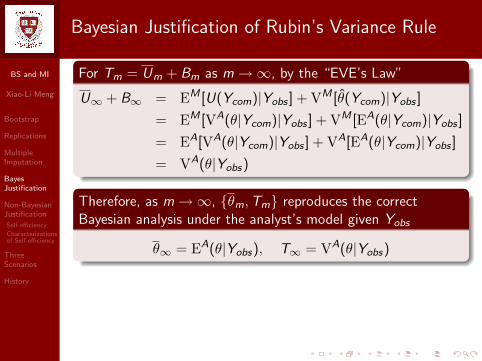
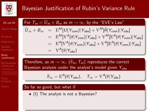
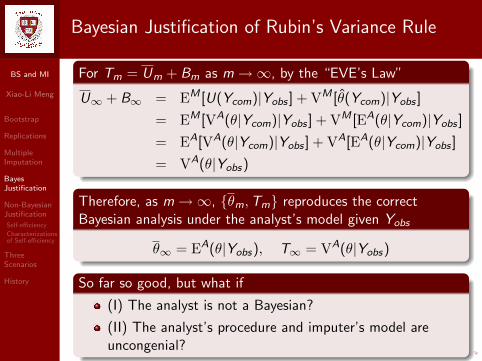
Bayesian Justification of Rubin’s Variance Rule
For Tm = Um + Bm as m→∞, by the “EVE’s Law”
U∞ + B∞ = EM [U(Ycom)|Yobs ] + VM [θ(Ycom)|Yobs ]
= EM [VA(θ|Ycom)|Yobs ] + VM [EA(θ|Ycom)|Yobs ]
= EA[VA(θ|Ycom)|Yobs ] + VA[EA(θ|Ycom)|Yobs ]
= VA(θ|Yobs)
Therefore, as m→∞, {θm,Tm} reproduces the correctBayesian analysis under the analyst’s model given Yobs
θ∞ = EA(θ|Yobs), T∞ = VA(θ|Yobs)
So far so good, but what if
(I) The analyst is not a Bayesian?
(II) The analyst’s procedure and imputer’s model areuncongenial?

BS and MI
Xiao-Li Meng
Bootstrap
Replications
MultipleImputation
BayesJustification
Non-BayesianJustification
Self-efficiency
Characterizationsof Self-efficiency
ThreeScenarios
History
Bayesian Justification of Rubin’s Variance Rule
For Tm = Um + Bm as m→∞, by the “EVE’s Law”
U∞ + B∞ = EM [U(Ycom)|Yobs ] + VM [θ(Ycom)|Yobs ]
= EM [VA(θ|Ycom)|Yobs ] + VM [EA(θ|Ycom)|Yobs ]
= EA[VA(θ|Ycom)|Yobs ] + VA[EA(θ|Ycom)|Yobs ]
= VA(θ|Yobs)
Therefore, as m→∞, {θm,Tm} reproduces the correctBayesian analysis under the analyst’s model given Yobs
θ∞ = EA(θ|Yobs), T∞ = VA(θ|Yobs)
So far so good, but what if
(I) The analyst is not a Bayesian?
(II) The analyst’s procedure and imputer’s model areuncongenial?
BS and MI
Xiao-Li Meng
Bootstrap
Replications
MultipleImputation
BayesJustification
Non-BayesianJustification
Self-efficiency
Characterizationsof Self-efficiency
ThreeScenarios
History
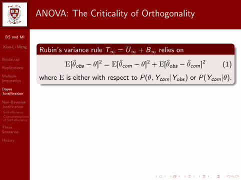
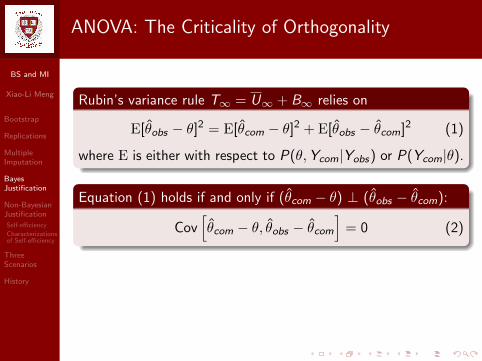
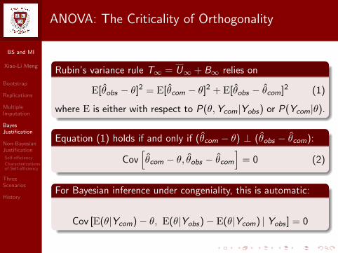
ANOVA: The Criticality of Orthogonality
Rubin’s variance rule T∞ = U∞ + B∞ relies on
E[θobs − θ]2 = E[θcom − θ]2 + E[θobs − θcom]2 (1)
where E is either with respect to P(θ,Ycom|Yobs) or P(Ycom|θ).
Equation (1) holds if and only if (θcom − θ) ⊥ (θobs − θcom):
Cov[θcom − θ, θobs − θcom
]= 0 (2)
For Bayesian inference under congeniality, this is automatic:
Cov [E(θ|Ycom)− θ, E(θ|Yobs)− E(θ|Ycom) | Yobs ] = 0
BS and MI
Xiao-Li Meng
Bootstrap
Replications
MultipleImputation
BayesJustification
Non-BayesianJustification
Self-efficiency
Characterizationsof Self-efficiency
ThreeScenarios
History
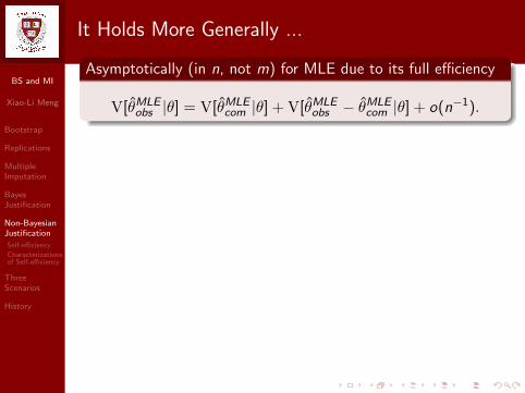
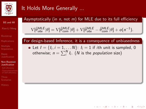
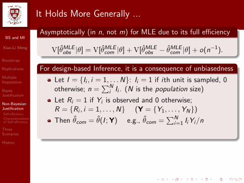
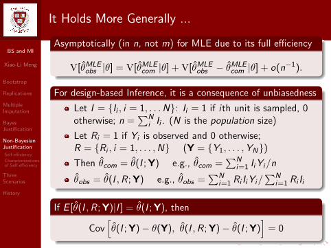
It Holds More Generally ...
Asymptotically (in n, not m) for MLE due to its full efficiency
V[θMLEobs |θ] = V[θMLE
com |θ] + V[θMLEobs − θMLE
com |θ] + o(n−1).
For design-based Inference, it is a consequence of unbiasedness
Let I = {Ii , i = 1, . . .N}: Ii = 1 if ith unit is sampled, 0otherwise; n =
∑Ni Ii . (N is the population size)
Let Ri = 1 if Yi is observed and 0 otherwise;R = {Ri , i = 1, . . . ,N} (Y = {Y1, . . . ,YN})Then θcom = θ(I ; Y) e.g., θcom =
∑Ni=1 IiYi/n
θobs = θ(I ,R; Y) e.g., θobs =∑N
i=1 Ri IiYi/∑N
i=1 Ri Ii
If E [θ(I ,R; Y)|I ] = θ(I ; Y), then
Cov[θ(I ; Y)− θ(Y), θ(I ,R; Y)− θ(I ; Y)
]= 0
BS and MI
Xiao-Li Meng
Bootstrap
Replications
MultipleImputation
BayesJustification
Non-BayesianJustification
Self-efficiency
Characterizationsof Self-efficiency
ThreeScenarios
History
It Holds More Generally ...
Asymptotically (in n, not m) for MLE due to its full efficiency
V[θMLEobs |θ] = V[θMLE
com |θ] + V[θMLEobs − θMLE
com |θ] + o(n−1).
For design-based Inference, it is a consequence of unbiasedness
Let I = {Ii , i = 1, . . .N}: Ii = 1 if ith unit is sampled, 0otherwise; n =
∑Ni Ii . (N is the population size)
Let Ri = 1 if Yi is observed and 0 otherwise;R = {Ri , i = 1, . . . ,N} (Y = {Y1, . . . ,YN})Then θcom = θ(I ; Y) e.g., θcom =
∑Ni=1 IiYi/n
θobs = θ(I ,R; Y) e.g., θobs =∑N
i=1 Ri IiYi/∑N
i=1 Ri Ii
If E [θ(I ,R; Y)|I ] = θ(I ; Y), then
Cov[θ(I ; Y)− θ(Y), θ(I ,R; Y)− θ(I ; Y)
]= 0

BS and MI
Xiao-Li Meng
Bootstrap
Replications
MultipleImputation
BayesJustification
Non-BayesianJustification
Self-efficiency
Characterizationsof Self-efficiency
ThreeScenarios
History
It Holds More Generally ...
Asymptotically (in n, not m) for MLE due to its full efficiency
V[θMLEobs |θ] = V[θMLE
com |θ] + V[θMLEobs − θMLE
com |θ] + o(n−1).
For design-based Inference, it is a consequence of unbiasedness
Let I = {Ii , i = 1, . . .N}: Ii = 1 if ith unit is sampled, 0otherwise; n =
∑Ni Ii . (N is the population size)
Let Ri = 1 if Yi is observed and 0 otherwise;R = {Ri , i = 1, . . . ,N} (Y = {Y1, . . . ,YN})
Then θcom = θ(I ; Y) e.g., θcom =∑N
i=1 IiYi/n
θobs = θ(I ,R; Y) e.g., θobs =∑N
i=1 Ri IiYi/∑N
i=1 Ri Ii
If E [θ(I ,R; Y)|I ] = θ(I ; Y), then
Cov[θ(I ; Y)− θ(Y), θ(I ,R; Y)− θ(I ; Y)
]= 0
BS and MI
Xiao-Li Meng
Bootstrap
Replications
MultipleImputation
BayesJustification
Non-BayesianJustification
Self-efficiency
Characterizationsof Self-efficiency
ThreeScenarios
History
It Holds More Generally ...
Asymptotically (in n, not m) for MLE due to its full efficiency
V[θMLEobs |θ] = V[θMLE
com |θ] + V[θMLEobs − θMLE
com |θ] + o(n−1).
For design-based Inference, it is a consequence of unbiasedness
Let I = {Ii , i = 1, . . .N}: Ii = 1 if ith unit is sampled, 0otherwise; n =
∑Ni Ii . (N is the population size)
Let Ri = 1 if Yi is observed and 0 otherwise;R = {Ri , i = 1, . . . ,N} (Y = {Y1, . . . ,YN})Then θcom = θ(I ; Y) e.g., θcom =
∑Ni=1 IiYi/n
θobs = θ(I ,R; Y) e.g., θobs =∑N
i=1 Ri IiYi/∑N
i=1 Ri Ii
If E [θ(I ,R; Y)|I ] = θ(I ; Y), then
Cov[θ(I ; Y)− θ(Y), θ(I ,R; Y)− θ(I ; Y)
]= 0

BS and MI
Xiao-Li Meng
Bootstrap
Replications
MultipleImputation
BayesJustification
Non-BayesianJustification
Self-efficiency
Characterizationsof Self-efficiency
ThreeScenarios
History
It Holds More Generally ...
Asymptotically (in n, not m) for MLE due to its full efficiency
V[θMLEobs |θ] = V[θMLE
com |θ] + V[θMLEobs − θMLE
com |θ] + o(n−1).
For design-based Inference, it is a consequence of unbiasedness
Let I = {Ii , i = 1, . . .N}: Ii = 1 if ith unit is sampled, 0otherwise; n =
∑Ni Ii . (N is the population size)
Let Ri = 1 if Yi is observed and 0 otherwise;R = {Ri , i = 1, . . . ,N} (Y = {Y1, . . . ,YN})Then θcom = θ(I ; Y) e.g., θcom =
∑Ni=1 IiYi/n
θobs = θ(I ,R; Y) e.g., θobs =∑N
i=1 Ri IiYi/∑N
i=1 Ri Ii
If E [θ(I ,R; Y)|I ] = θ(I ; Y), then
Cov[θ(I ; Y)− θ(Y), θ(I ,R; Y)− θ(I ; Y)
]= 0
BS and MI
Xiao-Li Meng
Bootstrap
Replications
MultipleImputation
BayesJustification
Non-BayesianJustification
Self-efficiency
Characterizationsof Self-efficiency
ThreeScenarios
History
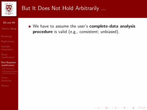
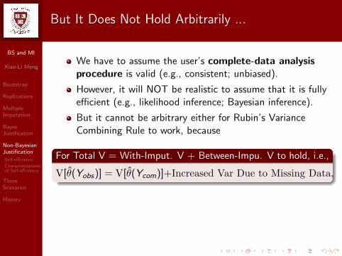
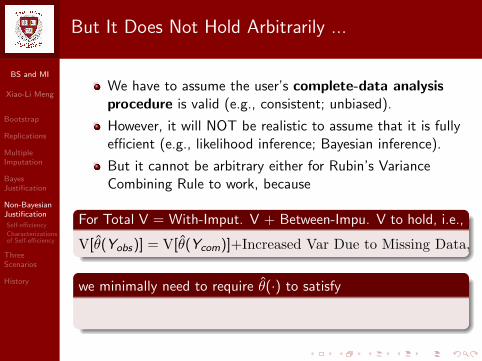
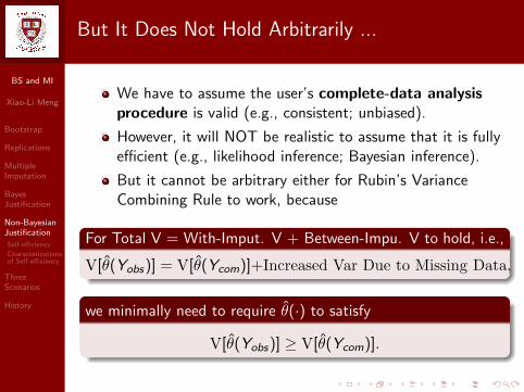
But It Does Not Hold Arbitrarily ...
We have to assume the user’s complete-data analysisprocedure is valid (e.g., consistent; unbiased).
However, it will NOT be realistic to assume that it is fullyefficient (e.g., likelihood inference; Bayesian inference).
But it cannot be arbitrary either for Rubin’s VarianceCombining Rule to work, because
For Total V = With-Imput. V + Between-Impu. V to hold, i.e.,
V[θ(Yobs)] = V[θ(Ycom)]+Increased Var Due to Missing Data,
we minimally need to require θ(·) to satisfy
V[θ(Yobs)] ≥ V[θ(Ycom)].
Wait! Is this Obvious???

BS and MI
Xiao-Li Meng
Bootstrap
Replications
MultipleImputation
BayesJustification
Non-BayesianJustification
Self-efficiency
Characterizationsof Self-efficiency
ThreeScenarios
History
But It Does Not Hold Arbitrarily ...
We have to assume the user’s complete-data analysisprocedure is valid (e.g., consistent; unbiased).
However, it will NOT be realistic to assume that it is fullyefficient (e.g., likelihood inference; Bayesian inference).
But it cannot be arbitrary either for Rubin’s VarianceCombining Rule to work, because
For Total V = With-Imput. V + Between-Impu. V to hold, i.e.,
V[θ(Yobs)] = V[θ(Ycom)]+Increased Var Due to Missing Data,
we minimally need to require θ(·) to satisfy
V[θ(Yobs)] ≥ V[θ(Ycom)].
Wait! Is this Obvious???
BS and MI
Xiao-Li Meng
Bootstrap
Replications
MultipleImputation
BayesJustification
Non-BayesianJustification
Self-efficiency
Characterizationsof Self-efficiency
ThreeScenarios
History
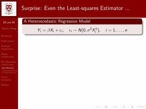
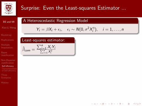
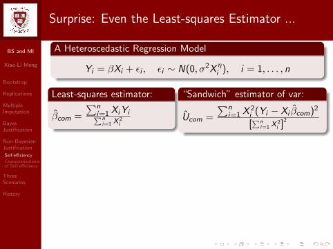
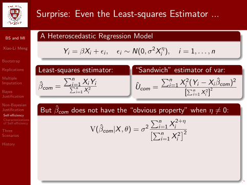
Surprise: Even the Least-squares Estimator ...
A Heteroscedastic Regression Model
Yi = βXi + εi , εi ∼ N(0, σ2X ηi ), i = 1, . . . , n
Least-squares estimator:
βcom =
∑ni=1 XiYi∑n
i=1 X 2i
“Sandwich” estimator of var:
Ucom =
∑ni=1 X 2
i (Yi − Xi βcom)2
[∑n
i=1 X 2i ]
2
But βcom does not have the “obvious property” when η 6= 0:
V(βcom|X , θ) = σ2
∑ni=1 X 2+η
i[∑ni=1 X 2
i
]2Compare, when η = 0:
V(βcom|X , θ) = σ2 1∑ni=1 X 2
i
BS and MI
Xiao-Li Meng
Bootstrap
Replications
MultipleImputation
BayesJustification
Non-BayesianJustification
Self-efficiency
Characterizationsof Self-efficiency
ThreeScenarios
History
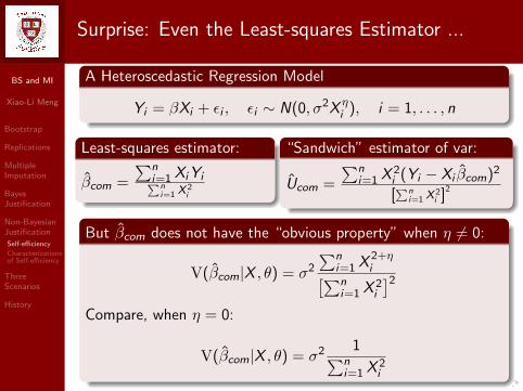
Surprise: Even the Least-squares Estimator ...
A Heteroscedastic Regression Model
Yi = βXi + εi , εi ∼ N(0, σ2X ηi ), i = 1, . . . , n
Least-squares estimator:
βcom =
∑ni=1 XiYi∑n
i=1 X 2i
“Sandwich” estimator of var:
Ucom =
∑ni=1 X 2
i (Yi − Xi βcom)2
[∑n
i=1 X 2i ]
2
But βcom does not have the “obvious property” when η 6= 0:
V(βcom|X , θ) = σ2
∑ni=1 X 2+η
i[∑ni=1 X 2
i
]2
Compare, when η = 0:
V(βcom|X , θ) = σ2 1∑ni=1 X 2
i
BS and MI
Xiao-Li Meng
Bootstrap
Replications
MultipleImputation
BayesJustification
Non-BayesianJustification
Self-efficiency
Characterizationsof Self-efficiency
ThreeScenarios
History
Surprise: Even the Least-squares Estimator ...
A Heteroscedastic Regression Model
Yi = βXi + εi , εi ∼ N(0, σ2X ηi ), i = 1, . . . , n
Least-squares estimator:
βcom =
∑ni=1 XiYi∑n
i=1 X 2i
“Sandwich” estimator of var:
Ucom =
∑ni=1 X 2
i (Yi − Xi βcom)2
[∑n
i=1 X 2i ]
2
But βcom does not have the “obvious property” when η 6= 0:
V(βcom|X , θ) = σ2
∑ni=1 X 2+η
i[∑ni=1 X 2
i
]2Compare, when η = 0:
V(βcom|X , θ) = σ2 1∑ni=1 X 2
i
BS and MI
Xiao-Li Meng
Bootstrap
Replications
MultipleImputation
BayesJustification
Non-BayesianJustification
Self-efficiency
Characterizationsof Self-efficiency
ThreeScenarios
History
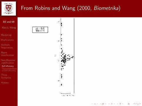
From Robins and Wang (2000, Biometrika)
BS and MI
Xiao-Li Meng
Bootstrap
Replications
MultipleImputation
BayesJustification
Non-BayesianJustification
Self-efficiency
Characterizationsof Self-efficiency
ThreeScenarios
History
Please Throw Away Some Data ...
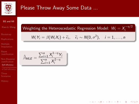
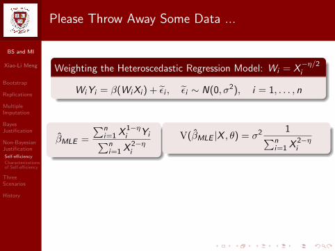
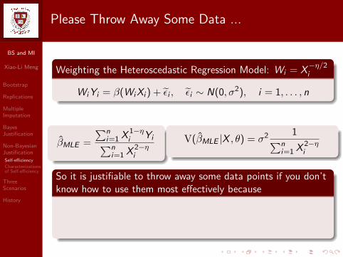
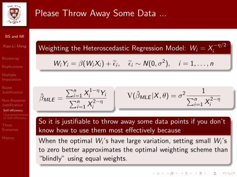
Weighting the Heteroscedastic Regression Model: Wi = X−η/2i
WiYi = β(WiXi ) + εi , εi ∼ N(0, σ2), i = 1, . . . , n
βMLE =
∑ni=1 X 1−η
i Yi∑ni=1 X 2−η
i
V(βMLE |X , θ) = σ2 1∑ni=1 X 2−η
i
So it is justifiable to throw away some data points if you don’tknow how to use them most effectively because
When the optimal Wi ’s have large variation, setting small Wi ’sto zero better approximates the optimal weighting scheme than“blindly” using equal weights.
BS and MI
Xiao-Li Meng
Bootstrap
Replications
MultipleImputation
BayesJustification
Non-BayesianJustification
Self-efficiency
Characterizationsof Self-efficiency
ThreeScenarios
History
Please Throw Away Some Data ...
Weighting the Heteroscedastic Regression Model: Wi = X−η/2i
WiYi = β(WiXi ) + εi , εi ∼ N(0, σ2), i = 1, . . . , n
βMLE =
∑ni=1 X 1−η
i Yi∑ni=1 X 2−η
i
V(βMLE |X , θ) = σ2 1∑ni=1 X 2−η
i
So it is justifiable to throw away some data points if you don’tknow how to use them most effectively because
When the optimal Wi ’s have large variation, setting small Wi ’sto zero better approximates the optimal weighting scheme than“blindly” using equal weights.
BS and MI
Xiao-Li Meng
Bootstrap
Replications
MultipleImputation
BayesJustification
Non-BayesianJustification
Self-efficiency
Characterizationsof Self-efficiency
ThreeScenarios
History
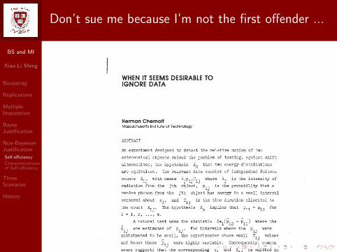
Don’t sue me because I’m not the first offender ...
BS and MI
Xiao-Li Meng
Bootstrap
Replications
MultipleImputation
BayesJustification
Non-BayesianJustification
Self-efficiency
Characterizationsof Self-efficiency
ThreeScenarios
History
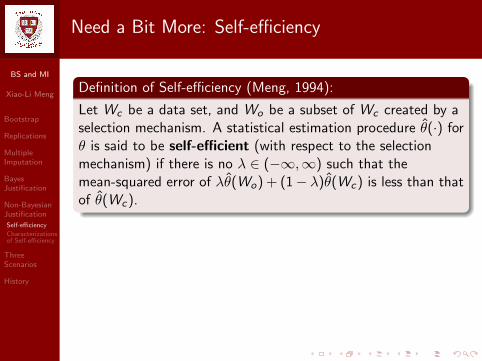
Need a Bit More: Self-efficiency
Definition of Self-efficiency (Meng, 1994):
Let Wc be a data set, and Wo be a subset of Wc created by aselection mechanism. A statistical estimation procedure θ(·) forθ is said to be self-efficient (with respect to the selectionmechanism) if there is no λ ∈ (−∞,∞) such that themean-squared error of λθ(Wo) + (1− λ)θ(Wc) is less than thatof θ(Wc).
Self-efficiency is a weaker requirement than full-efficiency(e.g., MLE, Bayesian procedures), but can be violated incommon practice. (Had I known that back in 1994 ...)
Under the assumption of Congeniality, self-efficiency is asufficient and necessary condition for Rubin’s variance ruleto hold (Meng, 1994).
BS and MI
Xiao-Li Meng
Bootstrap
Replications
MultipleImputation
BayesJustification
Non-BayesianJustification
Self-efficiency
Characterizationsof Self-efficiency
ThreeScenarios
History
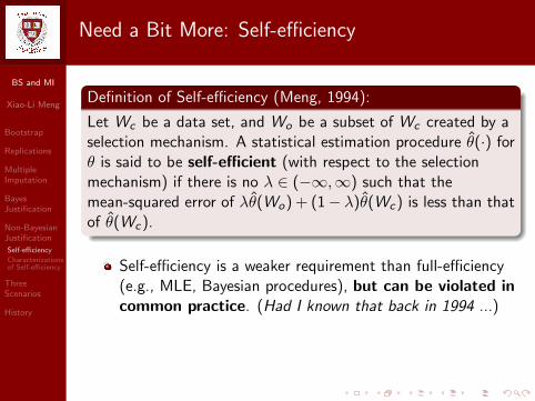
Need a Bit More: Self-efficiency
Definition of Self-efficiency (Meng, 1994):
Let Wc be a data set, and Wo be a subset of Wc created by aselection mechanism. A statistical estimation procedure θ(·) forθ is said to be self-efficient (with respect to the selectionmechanism) if there is no λ ∈ (−∞,∞) such that themean-squared error of λθ(Wo) + (1− λ)θ(Wc) is less than thatof θ(Wc).
Self-efficiency is a weaker requirement than full-efficiency(e.g., MLE, Bayesian procedures), but can be violated incommon practice. (Had I known that back in 1994 ...)
Under the assumption of Congeniality, self-efficiency is asufficient and necessary condition for Rubin’s variance ruleto hold (Meng, 1994).
BS and MI
Xiao-Li Meng
Bootstrap
Replications
MultipleImputation
BayesJustification
Non-BayesianJustification
Self-efficiency
Characterizationsof Self-efficiency
ThreeScenarios
History
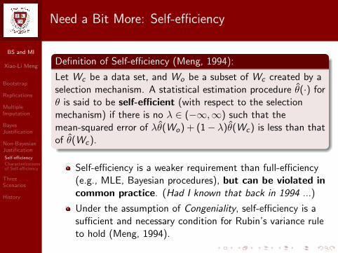
Need a Bit More: Self-efficiency
Definition of Self-efficiency (Meng, 1994):
Let Wc be a data set, and Wo be a subset of Wc created by aselection mechanism. A statistical estimation procedure θ(·) forθ is said to be self-efficient (with respect to the selectionmechanism) if there is no λ ∈ (−∞,∞) such that themean-squared error of λθ(Wo) + (1− λ)θ(Wc) is less than thatof θ(Wc).
Self-efficiency is a weaker requirement than full-efficiency(e.g., MLE, Bayesian procedures), but can be violated incommon practice. (Had I known that back in 1994 ...)
Under the assumption of Congeniality, self-efficiency is asufficient and necessary condition for Rubin’s variance ruleto hold (Meng, 1994).
BS and MI
Xiao-Li Meng
Bootstrap
Replications
MultipleImputation
BayesJustification
Non-BayesianJustification
Self-efficiency
Characterizationsof Self-efficiency
ThreeScenarios
History
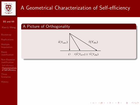
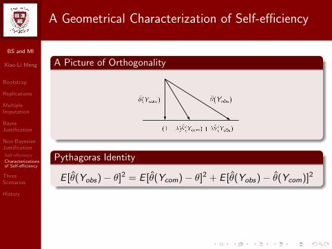
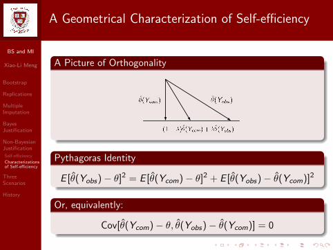
A Geometrical Characterization of Self-efficiency
A Picture of Orthogonality
Pythagoras Identity
E [θ(Yobs)− θ]2 = E [θ(Ycom)− θ]2 + E [θ(Yobs)− θ(Ycom)]2
Or, equivalently:
Cov[θ(Ycom)− θ, θ(Yobs)− θ(Ycom)] = 0
BS and MI
Xiao-Li Meng
Bootstrap
Replications
MultipleImputation
BayesJustification
Non-BayesianJustification
Self-efficiency
Characterizationsof Self-efficiency
ThreeScenarios
History
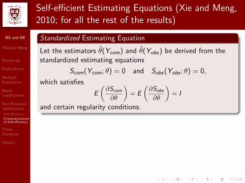
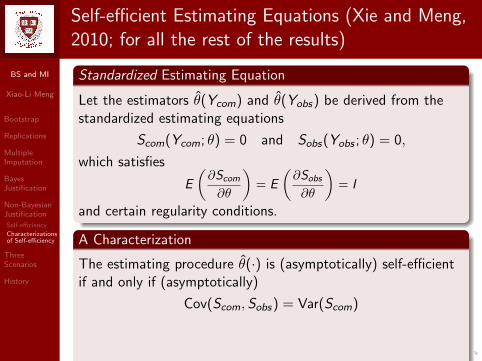
Self-efficient Estimating Equations (Xie and Meng,2010; for all the rest of the results)
Standardized Estimating Equation
Let the estimators θ(Ycom) and θ(Yobs) be derived from thestandardized estimating equations
Scom(Ycom; θ) = 0 and Sobs(Yobs ; θ) = 0,
which satisfies
E
(∂Scom
∂θ
)= E
(∂Sobs
∂θ
)= I
and certain regularity conditions.
A Characterization
The estimating procedure θ(·) is (asymptotically) self-efficientif and only if (asymptotically)
Cov(Scom,Sobs) = Var(Scom)
or, equivalently, “the regression coefficient”
B = Var(Scom)−1Cov(Scom,Sobs) = I .
BS and MI
Xiao-Li Meng
Bootstrap
Replications
MultipleImputation
BayesJustification
Non-BayesianJustification
Self-efficiency
Characterizationsof Self-efficiency
ThreeScenarios
History
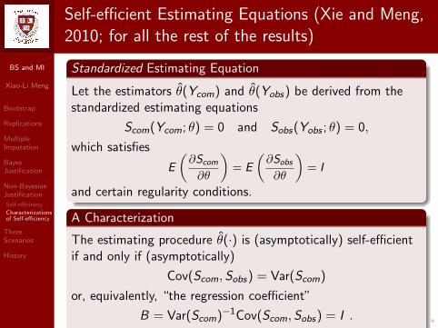
Self-efficient Estimating Equations (Xie and Meng,2010; for all the rest of the results)
Standardized Estimating Equation
Let the estimators θ(Ycom) and θ(Yobs) be derived from thestandardized estimating equations
Scom(Ycom; θ) = 0 and Sobs(Yobs ; θ) = 0,
which satisfies
E
(∂Scom
∂θ
)= E
(∂Sobs
∂θ
)= I
and certain regularity conditions.
A Characterization
The estimating procedure θ(·) is (asymptotically) self-efficientif and only if (asymptotically)
Cov(Scom, Sobs) = Var(Scom)
or, equivalently, “the regression coefficient”
B = Var(Scom)−1Cov(Scom,Sobs) = I .
BS and MI
Xiao-Li Meng
Bootstrap
Replications
MultipleImputation
BayesJustification
Non-BayesianJustification
Self-efficiency
Characterizationsof Self-efficiency
ThreeScenarios
History
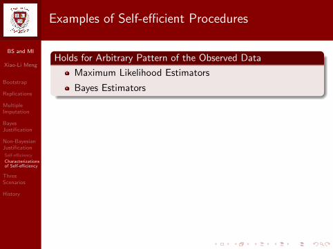
Examples of Self-efficient Procedures
Holds for Arbitrary Pattern of the Observed Data
Maximum Likelihood Estimators
Bayes Estimators
Holds for “Regular Pattern” of the Observed Data
Let the complete data Ycom be an i.i.d. sequence and Yobs bea regular subset of it, i.e.,
Ycom = (Y1, · · · ,Yn)
Yobs = (Yi1 , · · · ,Yim) .
Then any estimating equation having the form
S(Ycom; θ) =n∑
i=1
g(Yi ; θ)
is self-efficient.
BS and MI
Xiao-Li Meng
Bootstrap
Replications
MultipleImputation
BayesJustification
Non-BayesianJustification
Self-efficiency
Characterizationsof Self-efficiency
ThreeScenarios
History
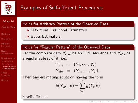
Examples of Self-efficient Procedures
Holds for Arbitrary Pattern of the Observed Data
Maximum Likelihood Estimators
Bayes Estimators
Holds for “Regular Pattern” of the Observed Data
Let the complete data Ycom be an i.i.d. sequence and Yobs bea regular subset of it, i.e.,
Ycom = (Y1, · · · ,Yn)
Yobs = (Yi1 , · · · ,Yim) .
Then any estimating equation having the form
S(Ycom; θ) =n∑
i=1
g(Yi ; θ)
is self-efficient.
BS and MI
Xiao-Li Meng
Bootstrap
Replications
MultipleImputation
BayesJustification
Non-BayesianJustification
Self-efficiency
Characterizationsof Self-efficiency
ThreeScenarios
History
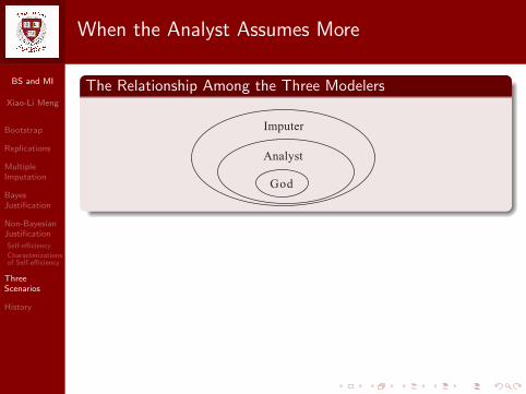
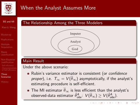
When the Analyst Assumes More
The Relationship Among the Three Modelers
����
�����
�����
Main Result
Under the above scenario:
Rubin’s variance estimator is consistent (or confidenceproper), i.e. T∞ = V (θ∞) asymptotically, if the analyst’sestimating procedure is self-efficient.
The MI estimator θ∞ is less efficient than the analyst’sobserved-data estimator θA
obs : V (θ∞) ≥ V (θAobs).

BS and MI
Xiao-Li Meng
Bootstrap
Replications
MultipleImputation
BayesJustification
Non-BayesianJustification
Self-efficiency
Characterizationsof Self-efficiency
ThreeScenarios
History
When the Analyst Assumes More
The Relationship Among the Three Modelers
����
�����
�����
Main Result
Under the above scenario:
Rubin’s variance estimator is consistent (or confidenceproper), i.e. T∞ = V (θ∞) asymptotically, if the analyst’sestimating procedure is self-efficient.
The MI estimator θ∞ is less efficient than the analyst’sobserved-data estimator θA
obs : V (θ∞) ≥ V (θAobs).

BS and MI
Xiao-Li Meng
Bootstrap
Replications
MultipleImputation
BayesJustification
Non-BayesianJustification
Self-efficiency
Characterizationsof Self-efficiency
ThreeScenarios
History
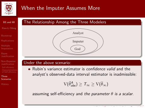
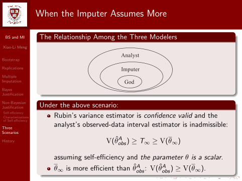
When the Imputer Assumes More
The Relationship Among the Three Modelers
����
�����
�����
Under the above scenario:
Rubin’s variance estimator is confidence valid and theanalyst’s observed-data interval estimator is inadmissible:
V(θAobs) ≥ T∞ ≥ V(θ∞)
assuming self-efficiency and the parameter θ is a scalar.
θ∞ is more efficient than θAobs : V(θA
obs) ≥ V(θ∞).
BS and MI
Xiao-Li Meng
Bootstrap
Replications
MultipleImputation
BayesJustification
Non-BayesianJustification
Self-efficiency
Characterizationsof Self-efficiency
ThreeScenarios
History
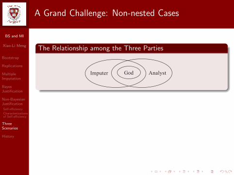
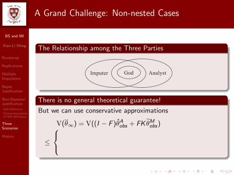
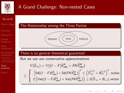
A Grand Challenge: Non-nested Cases
The Relationship among the Three Parties
��������� �����
There is no general theoretical guarantee!
But we can use conservative approximations
V(θ∞) = V((I − F )θAobs + FK θM
obs)
≤
[Sd((I − F )θA
obs) + Sd(FK θMobs)]2
≤(
U1/2
∞ + B1/2∞
)2
, scalar;
2(
Var((I − F )θAobs) + Var(FK θM
obs))≤ 2(U∞ + B∞), vector.
BS and MI
Xiao-Li Meng
Bootstrap
Replications
MultipleImputation
BayesJustification
Non-BayesianJustification
Self-efficiency
Characterizationsof Self-efficiency
ThreeScenarios
History
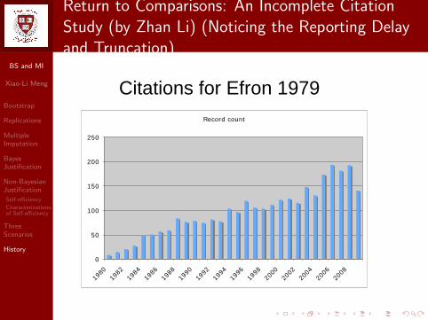
Return to Comparisons: An Incomplete CitationStudy (by Zhan Li) (Noticing the Reporting Delayand Truncation)
Citations for Efron 1979Record count
0
50
100
150
200
250
1980
1982
1984
1986
1988
1990
1992
1994
1996
1998
2000
2002
2004
2006
2008
BS and MI
Xiao-Li Meng
Bootstrap
Replications
MultipleImputation
BayesJustification
Non-BayesianJustification
Self-efficiency
Characterizationsof Self-efficiency
ThreeScenarios
History
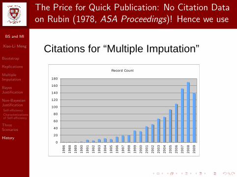
The Price for Quick Publication: No Citation Dataon Rubin (1978, ASA Proceedings)! Hence we use
Citations for “Multiple Imputation”
Record Count
0
20
40
60
80
100
120
140
160
180
1986
1988
1989
1990
1991
1992
1993
1994
1995
1996
1997
1998
1999
2000
2001
2002
2003
2004
2005
2006
2007
2008
2009
BS and MI
Xiao-Li Meng
Bootstrap
Replications
MultipleImputation
BayesJustification
Non-BayesianJustification
Self-efficiency
Characterizationsof Self-efficiency
ThreeScenarios
History
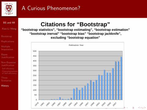
A Curious Phenomenon?
Citations for “Bootstrap” “bootstrap statistics”, “bootstrap estimating”, “bootstrap estimation”
“bootstrap inerval” “bootstrap bias” “bootstrap jackknife”, excluding “bootstrap equation”
Publication Year
0
50
100
150
200
250
300
350
400
450
500
1979
1981
1983
1985
1987
1989
1991
1993
1995
1997
1999
2001
2003
2005
2007

BS and MI
Xiao-Li Meng
Bootstrap
Replications
MultipleImputation
BayesJustification
Non-BayesianJustification
Self-efficiency
Characterizationsof Self-efficiency
ThreeScenarios
History
A Concluding Wisdom for Anyone Younger ThanMe
Be patient
Because there is a 12-year waiting period before fame ...

BS and MI
Xiao-Li Meng
Bootstrap
Replications
MultipleImputation
BayesJustification
Non-BayesianJustification
Self-efficiency
Characterizationsof Self-efficiency
ThreeScenarios
History
A Concluding Wisdom for Anyone Younger ThanMe
Be patient
Because there is a 12-year waiting period before fame ...


![arXiv:1602.07933v3 [stat.ME] 5 Dec 2016 modern estimators require bootstrapping to calculate con- ... [stat.ME] 5 Dec 2016. 2 In ... BOOTSTRAP INFERENCE WHEN USING MULTIPLE IMPUTATION](https://img.pdfslide.net/doc/110x75/5ae0f3187f8b9a8f298ed987/arxiv160207933v3-statme-5-dec-2016-modern-estimators-require-bootstrapping.jpg)