CHAPTER

31

ELECTROMAGNETIC OSCILLATIONS AND ALTERNATING CURRENT

31-1 What is Physics?

We have explored the basic physics of electric and magnetic fields and how energy can be stored in capacitors and inductors.

We next turn to the associated applied physics, in which the energy stored in one location can be transferred to another location

so that it can be put to use. For example, energy produced at a power plant can show up at your home to run a computer. The

total worth of this applied physics is now so high that its estimation is almost impossible. Indeed, modern civilization would be

impossible without this applied physics.

In most parts of the world, electrical energy is transferred not as a direct current but as a sinusoidally oscillating current

(alternating current, or ac). The challenge to both physicists and engineers is to design ac systems that transfer energy efficiently

and to build appliances that make use of that energy.

In our discussion of electrically oscillating systems in this chapter, our first step is to examine oscillations in a simple circuit

consisting of inductance L and capacitance C.

Copyright © 2011 John Wiley & Sons, Inc. All rights reserved.

31-2 LC Oscillations, Qualitatively

Of the three circuit elements resistance R, capacitance C, and inductance L, we have so far discussed the series combinations RC

(in Section 27-9) and RL (in Section 30-9). In these two kinds of circuit we found that the charge, current, and potential

difference grow and decay exponentially. The time scale of the growth or decay is given by a time constant τ, which is either

capacitive or inductive.

We now examine the remaining two-element circuit combination LC. You will see that in this case the charge, current, and

potential difference do not decay exponentially with time but vary sinusoidally (with period T and angular frequency ω). The

resulting oscillations of the capacitor's electric field and the inductor's magnetic field are said to be electromagnetic

oscillations. Such a circuit is said to oscillate.

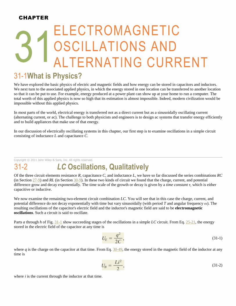
Parts a through h of Fig. 31-1 show succeeding stages of the oscillations in a simple LC circuit. From Eq. 25-21, the energy

stored in the electric field of the capacitor at any time is

(31-1)

where q is the charge on the capacitor at that time. From Eq. 30-49, the energy stored in the magnetic field of the inductor at any

time is

(31-2)

where i is the current through the inductor at that time.

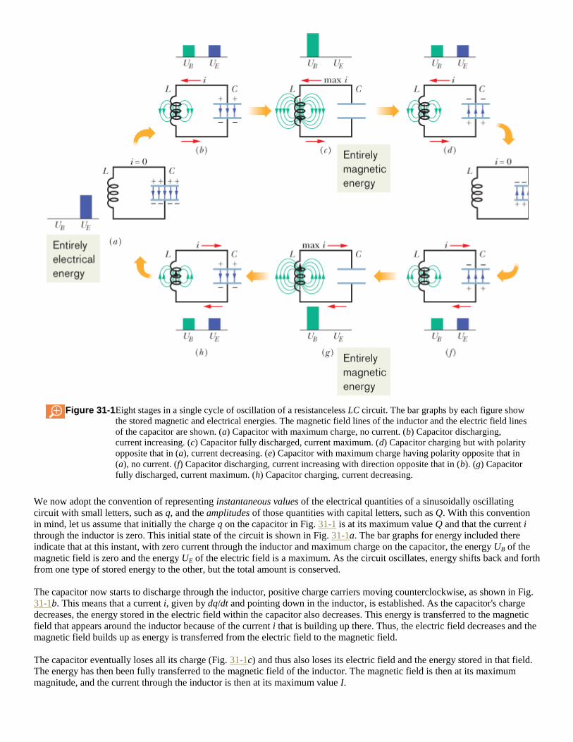
Figure 31-1 Eight stages in a single cycle of oscillation of a resistanceless LC circuit. The bar graphs by each figure show

the stored magnetic and electrical energies. The magnetic field lines of the inductor and the electric field lines

of the capacitor are shown. (a) Capacitor with maximum charge, no current. (b) Capacitor discharging,

current increasing. (c) Capacitor fully discharged, current maximum. (d) Capacitor charging but with polarity

opposite that in (a), current decreasing. (e) Capacitor with maximum charge having polarity opposite that in

(a), no current. (f) Capacitor discharging, current increasing with direction opposite that in (b). (g) Capacitor

fully discharged, current maximum. (h) Capacitor charging, current decreasing.

We now adopt the convention of representing instantaneous values of the electrical quantities of a sinusoidally oscillating

circuit with small letters, such as q, and the amplitudes of those quantities with capital letters, such as Q. With this convention

in mind, let us assume that initially the charge q on the capacitor in Fig. 31-1 is at its maximum value Q and that the current i

through the inductor is zero. This initial state of the circuit is shown in Fig. 31-1a. The bar graphs for energy included there

indicate that at this instant, with zero current through the inductor and maximum charge on the capacitor, the energy UB of the

magnetic field is zero and the energy UE of the electric field is a maximum. As the circuit oscillates, energy shifts back and forth

from one type of stored energy to the other, but the total amount is conserved.

The capacitor now starts to discharge through the inductor, positive charge carriers moving counterclockwise, as shown in Fig.

31-1b. This means that a current i, given by dq/dt and pointing down in the inductor, is established. As the capacitor's charge

decreases, the energy stored in the electric field within the capacitor also decreases. This energy is transferred to the magnetic

field that appears around the inductor because of the current i that is building up there. Thus, the electric field decreases and the

magnetic field builds up as energy is transferred from the electric field to the magnetic field.

The capacitor eventually loses all its charge (Fig. 31-1c) and thus also loses its electric field and the energy stored in that field.

The energy has then been fully transferred to the magnetic field of the inductor. The magnetic field is then at its maximum

magnitude, and the current through the inductor is then at its maximum value I.

Although the charge on the capacitor is now zero, the counterclockwise current must continue because the inductor does not

allow it to change suddenly to zero. The current continues to transfer positive charge from the top plate to the bottom plate

through the circuit (Fig. 31-1d). Energy now flows from the inductor back to the capacitor as the electric field within the

capacitor builds up again. The current gradually decreases during this energy transfer. When, eventually, the energy has been

transferred completely back to the capacitor (Fig. 31-1e), the current has decreased to zero (momentarily). The situation of Fig.

31-1e is like the initial situation, except that the capacitor is now charged oppositely.

The capacitor then starts to discharge again but now with a clockwise current (Fig. 31-1f). Reasoning as before, we see that the

clockwise current builds to a maximum (Fig. 31-1g) and then decreases (Fig. 31-1h), until the circuit eventually returns to its

initial situation (Fig. 31-1a). The process then repeats at some frequency f and thus at an angular frequency ω = 2πf. In the ideal

LC circuit with no resistance, there are no energy transfers other than that between the electric field of the capacitor and the

magnetic field of the inductor. Because of the conservation of energy, the oscillations continue indefinitely. The oscillations

need not begin with the energy all in the electric field; the initial situation could be any other stage of the oscillation.

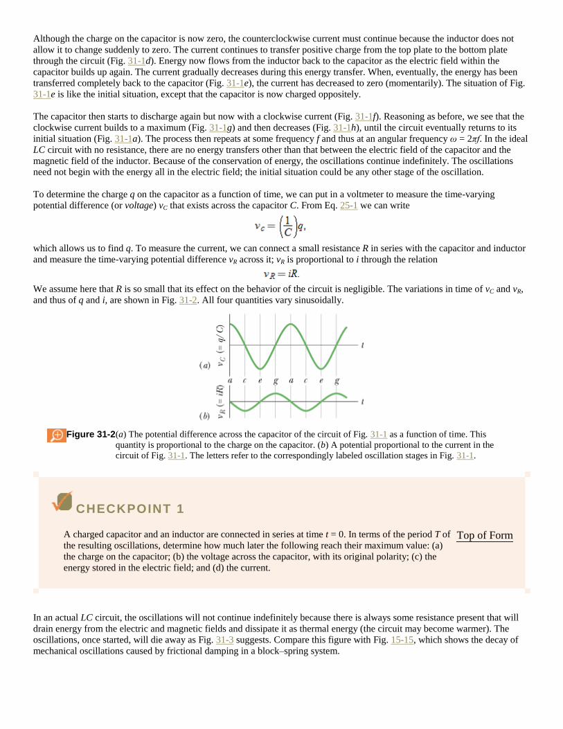
To determine the charge q on the capacitor as a function of time, we can put in a voltmeter to measure the time-varying

potential difference (or voltage) vC that exists across the capacitor C. From Eq. 25-1 we can write

which allows us to find q. To measure the current, we can connect a small resistance R in series with the capacitor and inductor

and measure the time-varying potential difference vR across it; vR is proportional to i through the relation

We assume here that R is so small that its effect on the behavior of the circuit is negligible. The variations in time of vC and vR,

and thus of q and i, are shown in Fig. 31-2. All four quantities vary sinusoidally.

Figure 31-2 (a) The potential difference across the capacitor of the circuit of Fig. 31-1 as a function of time. This

quantity is proportional to the charge on the capacitor. (b) A potential proportional to the current in the

circuit of Fig. 31-1. The letters refer to the correspondingly labeled oscillation stages in Fig. 31-1.

CHECKPOINT 1

A charged capacitor and an inductor are connected in series at time t = 0. In terms of the period T of

the resulting oscillations, determine how much later the following reach their maximum value: (a)

the charge on the capacitor; (b) the voltage across the capacitor, with its original polarity; (c) the

energy stored in the electric field; and (d) the current.

Top of Form

In an actual LC circuit, the oscillations will not continue indefinitely because there is always some resistance present that will

drain energy from the electric and magnetic fields and dissipate it as thermal energy (the circuit may become warmer). The oscillations, once started, will die away as Fig. 31-3 suggests. Compare this figure with Fig. 15-15, which shows the decay of

mechanical oscillations caused by frictional damping in a block–spring system.

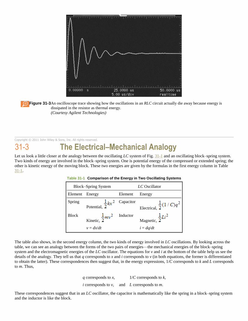
Figure 31-3 An oscilloscope trace showing how the oscillations in an RLC circuit actually die away because energy is

dissipated in the resistor as thermal energy.

(Courtesy Agilent Technologies)

Copyright © 2011 John Wiley & Sons, Inc. All rights reserved.

31-3 The Electrical–Mechanical Analogy

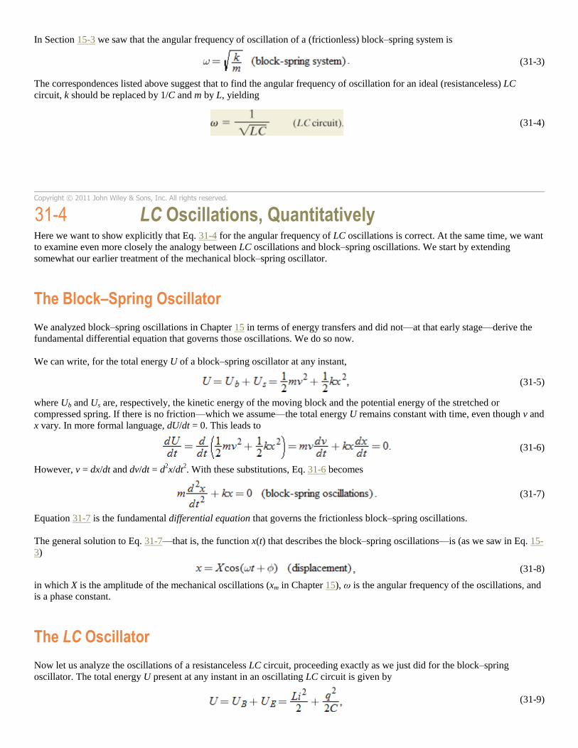
Let us look a little closer at the analogy between the oscillating LC system of Fig. 31-1 and an oscillating block–spring system.

Two kinds of energy are involved in the block–spring system. One is potential energy of the compressed or extended spring; the

other is kinetic energy of the moving block. These two energies are given by the formulas in the first energy column in Table

31-1.

Table 31-1 Comparison of the Energy in Two Oscillating Systems

Block–Spring System LC Oscillator

Element Energy Element Energy

Spring

Potential,

Capacitor

Electrical,

Block

Kinetic,

Inductor

Magnetic,

v = dx/dt i = dq/dt

The table also shows, in the second energy column, the two kinds of energy involved in LC oscillations. By looking across the

table, we can see an analogy between the forms of the two pairs of energies—the mechanical energies of the block–spring

system and the electromagnetic energies of the LC oscillator. The equations for v and i at the bottom of the table help us see the

details of the analogy. They tell us that q corresponds to x and i corresponds to v (in both equations, the former is differentiated

to obtain the latter). These correspondences then suggest that, in the energy expressions, 1/C corresponds to k and L corresponds

to m. Thus,

q corresponds to x, 1/C corresponds to k,

i corresponds to v, and L corresponds to m.

These correspondences suggest that in an LC oscillator, the capacitor is mathematically like the spring in a block–spring system

and the inductor is like the block.

In Section 15-3 we saw that the angular frequency of oscillation of a (frictionless) block–spring system is

(31-3)

The correspondences listed above suggest that to find the angular frequency of oscillation for an ideal (resistanceless) LC

circuit, k should be replaced by 1/C and m by L, yielding

(31-4)

Copyright © 2011 John Wiley & Sons, Inc. All rights reserved.

31-4 LC Oscillations, Quantitatively

Here we want to show explicitly that Eq. 31-4 for the angular frequency of LC oscillations is correct. At the same time, we want

to examine even more closely the analogy between LC oscillations and block–spring oscillations. We start by extending

somewhat our earlier treatment of the mechanical block–spring oscillator.

The Block–Spring Oscillator

We analyzed block–spring oscillations in Chapter 15 in terms of energy transfers and did not—at that early stage—derive the

fundamental differential equation that governs those oscillations. We do so now.

We can write, for the total energy U of a block–spring oscillator at any instant,

(31-5)

where Ub and Us are, respectively, the kinetic energy of the moving block and the potential energy of the stretched or

compressed spring. If there is no friction—which we assume—the total energy U remains constant with time, even though v and

x vary. In more formal language, dU/dt = 0. This leads to

(31-6)

However, v = dx/dt and dv/dt = d2x/dt

2. With these substitutions, Eq. 31-6 becomes

(31-7)

Equation 31-7 is the fundamental differential equation that governs the frictionless block–spring oscillations.

The general solution to Eq. 31-7—that is, the function x(t) that describes the block–spring oscillations—is (as we saw in Eq. 15-

3)

(31-8)

in which X is the amplitude of the mechanical oscillations (xm in Chapter 15), ω is the angular frequency of the oscillations, and

is a phase constant.

The LC Oscillator

Now let us analyze the oscillations of a resistanceless LC circuit, proceeding exactly as we just did for the block–spring

oscillator. The total energy U present at any instant in an oscillating LC circuit is given by

(31-9)

in which UB is the energy stored in the magnetic field of the inductor and UE is the energy stored in the electric field of the

capacitor. Since we have assumed the circuit resistance to be zero, no energy is transferred to thermal energy and U remains

constant with time. In more formal language, dU/dt must be zero. This leads to

(31-10)

However, i = dq/dt and di/dt = d2q/dt

2. With these substitutions, Eq. 31-10 becomes

(31-11)

This is the differential equation that describes the oscillations of a resistanceless LC circuit. Equations 31-11 and 31-7 are

exactly of the same mathematical form.

Charge and Current Oscillations

Since the differential equations are mathematically identical, their solutions must also be mathematically identical. Because q

corresponds to x, we can write the general solution of Eq. 31-11, by analogy to Eq. 31-8, as

(31-12)

where Q is the amplitude of the charge variations, ω is the angular frequency of the electromagnetic oscillations, and is the

phase constant.

Taking the first derivative of Eq. 31-12 with respect to time gives us the current of the LC oscillator:

(31-13)

The amplitude I of this sinusoidally varying current is

(31-14)

and so we can rewrite Eq. 31-13 as

(31-15)

Angular Frequencies

We can test whether Eq. 31-12 is a solution of Eq. 31-11 by substituting Eq. 31-12 and its second derivative with respect to time

into Eq. 31-11. The first derivative of Eq. 31-12 is Eq. 31-13. The second derivative is then

Substituting for q and d2q/dt

2 in Eq. 31-11, we obtain

Canceling Q cos(ωt + ) and rearranging lead to

Thus, Eq. 31-12 is indeed a solution of Eq. 31-11 if ω has the constant value . Note that this expression for ω is exactly

that given by Eq. 31-4, which we arrived at by examining correspondences.

The phase constant in Eq. 31-12 is determined by the conditions that exist at any certain time—say, t = 0. If the conditions yield

= 0 at t = 0, Eq. 31-12 requires that q = Q and Eq. 31-13 requires that i = 0; these are the initial conditions represented by Fig.

31-1a.

Electrical and Magnetic Energy Oscillations

The electrical energy stored in the LC circuit at time t is, from Eqs. 31-1 and 31-12,

(31-16)

The magnetic energy is, from Eqs. 31-2 and 31-13,

Substituting for ω from Eq. 31-4 then gives us

(31-17)

Figure 31-4 shows plots of UE(t) and UB(t) for the case of = 0. Note that

1. The maximum values of UE and UB are both Q2/2C.

2. At any instant the sum of UE and UB is equal to Q2/2C, a constant.

3. When UE is maximum, UB is zero, and conversely.

Figure 31-4 The stored magnetic energy and electrical energy in the circuit of Fig. 31-1 as a function of time. Note that

their sum remains constant. T is the period of oscillation.

CHECKPOINT 2

A capacitor in an LC oscillator has a maximum potential difference of 17 V and a maximum energy

of 160 μJ. When the capacitor has a potential difference of 5 V and an energy of 10 μJ, what are (a)

the emf across the inductor and (b) the energy stored in the magnetic field?

Top of Form

Sample Problem

LC oscillator: potential change, rate of current change

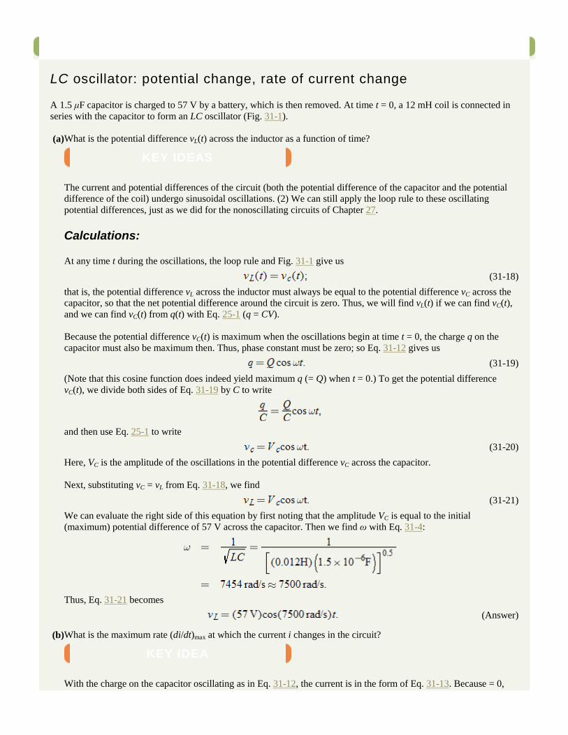
A 1.5 μF capacitor is charged to 57 V by a battery, which is then removed. At time t = 0, a 12 mH coil is connected in

series with the capacitor to form an LC oscillator (Fig. 31-1).

(a) What is the potential difference vL(t) across the inductor as a function of time?

KEY IDEAS

The current and potential differences of the circuit (both the potential difference of the capacitor and the potential

difference of the coil) undergo sinusoidal oscillations. (2) We can still apply the loop rule to these oscillating

potential differences, just as we did for the nonoscillating circuits of Chapter 27.

Calculations:

At any time t during the oscillations, the loop rule and Fig. 31-1 give us

(31-18)

that is, the potential difference vL across the inductor must always be equal to the potential difference vC across the

capacitor, so that the net potential difference around the circuit is zero. Thus, we will find vL(t) if we can find vC(t),

and we can find vC(t) from q(t) with Eq. 25-1 (q = CV).

Because the potential difference vC(t) is maximum when the oscillations begin at time t = 0, the charge q on the

capacitor must also be maximum then. Thus, phase constant must be zero; so Eq. 31-12 gives us

(31-19)

(Note that this cosine function does indeed yield maximum q (= Q) when t = 0.) To get the potential difference

vC(t), we divide both sides of Eq. 31-19 by C to write

and then use Eq. 25-1 to write

(31-20)

Here, VC is the amplitude of the oscillations in the potential difference vC across the capacitor.

Next, substituting vC = vL from Eq. 31-18, we find

(31-21)

We can evaluate the right side of this equation by first noting that the amplitude VC is equal to the initial

(maximum) potential difference of 57 V across the capacitor. Then we find ω with Eq. 31-4:

Thus, Eq. 31-21 becomes

(Answer)

(b) What is the maximum rate (di/dt)max at which the current i changes in the circuit?

KEY IDEA

With the charge on the capacitor oscillating as in Eq. 31-12, the current is in the form of Eq. 31-13. Because = 0,

that equation gives us

Calculations:

Taking the derivative, we have

We can simplify this equation by substituting CVC for Q (because we know C and VC but not Q) and for ω

according to Eq. 31-4. We get

This tells us that the current changes at a varying (sinusoidal) rate, with its maximum rate of change being

(Answer)

Copyright © 2011 John Wiley & Sons, Inc. All rights reserved.

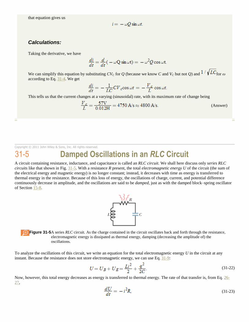
31-5 Damped Oscillations in an RLC Circuit

A circuit containing resistance, inductance, and capacitance is called an RLC circuit. We shall here discuss only series RLC

circuits like that shown in Fig. 31-5. With a resistance R present, the total electromagnetic energy U of the circuit (the sum of

the electrical energy and magnetic energy) is no longer constant; instead, it decreases with time as energy is transferred to

thermal energy in the resistance. Because of this loss of energy, the oscillations of charge, current, and potential difference

continuously decrease in amplitude, and the oscillations are said to be damped, just as with the damped block–spring oscillator

of Section 15-8.

Figure 31-5 A series RLC circuit. As the charge contained in the circuit oscillates back and forth through the resistance,

electromagnetic energy is dissipated as thermal energy, damping (decreasing the amplitude of) the

oscillations.

To analyze the oscillations of this circuit, we write an equation for the total electromagnetic energy U in the circuit at any

instant. Because the resistance does not store electromagnetic energy, we can use Eq. 31-9:

(31-22)

Now, however, this total energy decreases as energy is transferred to thermal energy. The rate of that transfer is, from Eq. 26-

27,

(31-23)

where the minus sign indicates that U decreases. By differentiating Eq. 31-22 with respect to time and then substituting the

result in Eq. 31-23, we obtain

Substituting dq/dt for i and d2q/dt

2 for di/dt, we obtain

(31-24)

which is the differential equation for damped oscillations in an RLC circuit.

The solution to Eq. 31-24 is

(31-25)

in which

(31-26)

where , as with an undamped oscillator. Equation 31-25 tells us how the charge on the capacitor oscillates in a

damped RLC circuit; that equation is the electromagnetic counterpart of Eq. 15-42, which gives the displacement of a damped

block–spring oscillator.

Equation 31-25 describes a sinusoidal oscillation (the cosine function) with an exponentially decaying amplitude Qe-Rt/2L

(the

factor that multiplies the cosine). The angular frequency ω′ of the damped oscillations is always less than the angular frequency

ω of the undamped oscillations; however, we shall here consider only situations in which R is small enough for us to replace ω′

with ω.

Let us next find an expression for the total electromagnetic energy U of the circuit as a function of time. One way to do so is to

monitor the energy of the electric field in the capacitor, which is given by Eq. 31-1 (UE = q2/2C). By substituting Eq. 31-25 into

Eq. 31-1, we obtain

(31-27)

Thus, the energy of the electric field oscillates according to a cosine-squared term, and the amplitude of that oscillation

decreases exponentially with time.

Sample Problem

Damped RLC circuit: charge amplitude

A series RLC circuit has inductance L = 12 mH, capacitance C = 1.6 μF, and resistance R = 1.5 Ω and begins to

oscillate at time t = 0.

(a) At what time t will the amplitude of the charge oscillations in the circuit be 50% of its initial value? (Note that we

do not know that initial value.)

KEY IDEA

The amplitude of the charge oscillations decreases exponentially with time t: According to Eq. 31-25, the charge

amplitude at any time t is Qe-Rt/2L

, in which Q is the amplitude at time t = 0.

Calculations:

We want the time when the charge amplitude has decreased to 0.50Q, that is, when

We can now cancel Q (which also means that we can answer the question without knowing the initial charge).

Taking the natural logarithms of both sides (to eliminate the exponential function), we have

Solving for t and then substituting given data yield

(Answer)

(b) How many oscillations are completed within this time?

KEY IDEA

The time for one complete oscillation is the period T = 2π/ω, where the angular frequency for LC oscillations is

given by Eq. 31-4 .

Calculation:

In the time interval Δt = 0.0111 s, the number of complete oscillations is

(Answer)

Thus, the amplitude decays by 50% in about 13 complete oscillations. This damping is less severe than that shown

in Fig. 31-3, where the amplitude decays by a little more than 50% in one oscillation.

Copyright © 2011 John Wiley & Sons, Inc. All rights reserved.

31-6 Alternating Current

The oscillations in an RLC circuit will not damp out if an external emf device supplies enough energy to make up for the energy

dissipated as thermal energy in the resistance R. Circuits in homes, offices, and factories, including countless RLC circuits,

receive such energy from local power companies. In most countries the energy is supplied via oscillating emfs and currents—

the current is said to be an alternating current, or ac for short. (The nonoscillating current from a battery is said to be a direct

current, or dc.) These oscillating emfs and currents vary sinusoidally with time, reversing direction (in North America) 120

times per second and thus having frequency f = 60 Hz.

At first sight this may seem to be a strange arrangement. We have seen that the drift speed of the conduction electrons in

household wiring may typically be 4 × 10-5 m/s

. If we now reverse their direction every , such electrons can move only

about 3 × 10-7

m in a half-cycle. At this rate, a typical electron can drift past no more than about 10 atoms in the wiring before it

is required to reverse its direction. How, you may wonder, can the electron ever get anywhere?

Although this question may be worrisome, it is a needless concern. The conduction electrons do not have to “get anywhere.”

When we say that the current in a wire is one ampere, we mean that charge passes through any plane cutting across that wire at

the rate of one coulomb per second. The speed at which the charge carriers cross that plane does not matter directly; one ampere

may correspond to many charge carriers moving very slowly or to a few moving very rapidly. Furthermore, the signal to the

electrons to reverse directions—which originates in the alternating emf provided by the power company's generator—is

propagated along the conductor at a speed close to that of light. All electrons, no matter where they are located, get their

reversal instructions at about the same instant. Finally, we note that for many devices, such as lightbulbs and toasters, the

direction of motion is unimportant as long as the electrons do move so as to transfer energy to the device via collisions with

atoms in the device.

The basic advantage of alternating current is this: As the current alternates, so does the magnetic field that surrounds the

conductor. This makes possible the use of Faraday's law of induction, which, among other things, means that we can step up

(increase) or step down (decrease) the magnitude of an alternating potential difference at will, using a device called a

transformer, as we shall discuss later. Moreover, alternating current is more readily adaptable to rotating machinery such as

generators and motors than is (nonalternating) direct current.

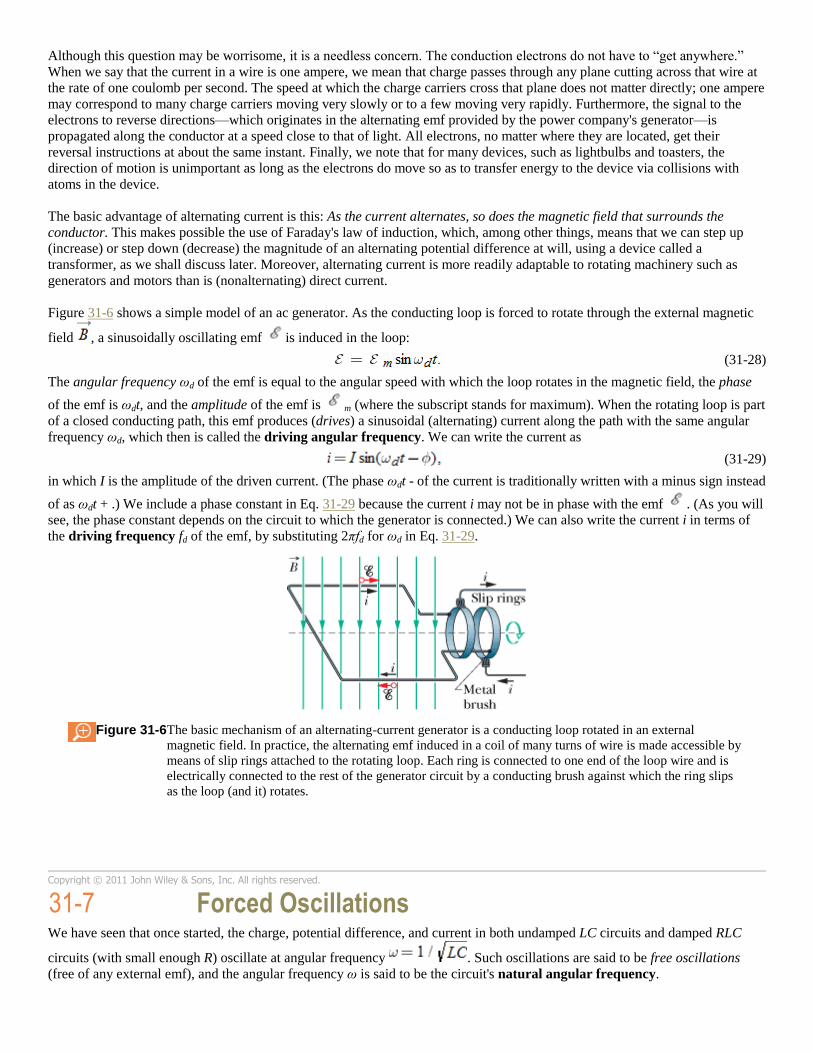
Figure 31-6 shows a simple model of an ac generator. As the conducting loop is forced to rotate through the external magnetic

field , a sinusoidally oscillating emf is induced in the loop:

(31-28)

The angular frequency ωd of the emf is equal to the angular speed with which the loop rotates in the magnetic field, the phase

of the emf is ωdt, and the amplitude of the emf is m (where the subscript stands for maximum). When the rotating loop is part

of a closed conducting path, this emf produces (drives) a sinusoidal (alternating) current along the path with the same angular

frequency ωd, which then is called the driving angular frequency. We can write the current as

(31-29)

in which I is the amplitude of the driven current. (The phase ωdt - of the current is traditionally written with a minus sign instead

of as ωdt + .) We include a phase constant in Eq. 31-29 because the current i may not be in phase with the emf . (As you will

see, the phase constant depends on the circuit to which the generator is connected.) We can also write the current i in terms of

the driving frequency fd of the emf, by substituting 2πfd for ωd in Eq. 31-29.

Figure 31-6 The basic mechanism of an alternating-current generator is a conducting loop rotated in an external

magnetic field. In practice, the alternating emf induced in a coil of many turns of wire is made accessible by

means of slip rings attached to the rotating loop. Each ring is connected to one end of the loop wire and is

electrically connected to the rest of the generator circuit by a conducting brush against which the ring slips

as the loop (and it) rotates.

Copyright © 2011 John Wiley & Sons, Inc. All rights reserved.

31-7 Forced Oscillations

We have seen that once started, the charge, potential difference, and current in both undamped LC circuits and damped RLC

circuits (with small enough R) oscillate at angular frequency . Such oscillations are said to be free oscillations

(free of any external emf), and the angular frequency ω is said to be the circuit's natural angular frequency.

When the external alternating emf of Eq. 31-28 is connected to an RLC circuit, the oscillations of charge, potential difference,

and current are said to be driven oscillations or forced oscillations. These oscillations always occur at the driving angular

frequency ωd:

Whatever the natural angular frequency ω of a circuit may be, forced oscillations of charge, current, and

potential difference in the circuit always occur at the driving angular frequency ωd.

However, as you will see in Section 31-9, the amplitudes of the oscillations very much depend on how close ωd is to ω. When

the two angular frequencies match—a condition known as resonance—the amplitude I of the current in the circuit is maximum.

Copyright © 2011 John Wiley & Sons, Inc. All rights reserved.

31-8 Three Simple Circuits

Later in this chapter, we shall connect an external alternating emf device to a series RLC circuit as in Fig. 31-7. We shall then

find expressions for the amplitude I and phase constant of the sinusoidally oscillating current in terms of the amplitude m and

angular frequency ωd of the external emf. First, let's consider three simpler circuits, each having an external emf and only one

other circuit element: R, C, or L. We start with a resistive element (a purely resistive load).

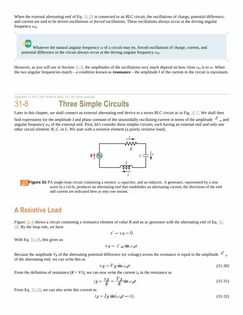
Figure 31-7 A single-loop circuit containing a resistor, a capacitor, and an inductor. A generator, represented by a sine

wave in a circle, produces an alternating emf that establishes an alternating current; the directions of the emf

and current are indicated here at only one instant.

A Resistive Load

Figure 31-8 shows a circuit containing a resistance element of value R and an ac generator with the alternating emf of Eq. 31-

28. By the loop rule, we have

With Eq. 31-28, this gives us

Because the amplitude VR of the alternating potential difference (or voltage) across the resistance is equal to the amplitude m

of the alternating emf, we can write this as

(31-30)

From the definition of resistance (R = V/i), we can now write the current iR in the resistance as

(31-31)

From Eq. 31-29, we can also write this current as

(31-32)

where IR is the amplitude of the current iR in the resistance. Comparing Eqs. 31-31 and 31-32, we see that for a purely resistive

load the phase constant = 0°. We also see that the voltage amplitude and current amplitude are related by

(31-33)

Although we found this relation for the circuit of Fig. 31-8, it applies to any resistance in any ac circuit.

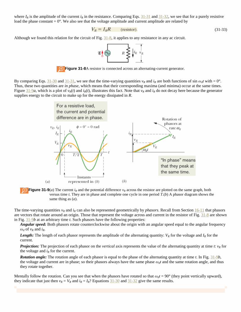
Figure 31-8 A resistor is connected across an alternating-current generator.

By comparing Eqs. 31-30 and 31-31, we see that the time-varying quantities vR and iR are both functions of sin ωdt with = 0°.

Thus, these two quantities are in phase, which means that their corresponding maxima (and minima) occur at the same times.

Figure 31-9a, which is a plot of vR(t) and iR(t), illustrates this fact. Note that vR and iR do not decay here because the generator

supplies energy to the circuit to make up for the energy dissipated in R.

Figure 31-9 (a) The current iR and the potential difference vR across the resistor are plotted on the same graph, both

versus time t. They are in phase and complete one cycle in one period T.(b) A phasor diagram shows the

same thing as (a).

The time-varying quantities vR and iR can also be represented geometrically by phasors. Recall from Section 16-11 that phasors

are vectors that rotate around an origin. Those that represent the voltage across and current in the resistor of Fig. 31-8 are shown

in Fig. 31-9b at an arbitrary time t. Such phasors have the following properties:

Angular speed: Both phasors rotate counterclockwise about the origin with an angular speed equal to the angular frequency

ωd of vR and iR.

Length: The length of each phasor represents the amplitude of the alternating quantity: VR for the voltage and IR for the

current.

Projection: The projection of each phasor on the vertical axis represents the value of the alternating quantity at time t: vR for

the voltage and iR for the current.

Rotation angle: The rotation angle of each phasor is equal to the phase of the alternating quantity at time t. In Fig. 31-9b,

the voltage and current are in phase; so their phasors always have the same phase ωdt and the same rotation angle, and thus

they rotate together.

Mentally follow the rotation. Can you see that when the phasors have rotated so that ωdt = 90° (they point vertically upward),

they indicate that just then vR = VR and iR = IR? Equations 31-30 and 31-32 give the same results.

CHECKPOINT 3

If we increase the driving frequency in a circuit with a purely resistive load, do (a) amplitude VR and

(b) amplitude IR increase, decrease, or remain the same? Top of Form

Sample Problem

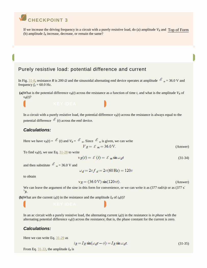
Purely resistive load: potential difference and current

In Fig. 31-8, resistance R is 200 Ω and the sinusoidal alternating emf device operates at amplitude m = 36.0 V and

frequency fd = 60.0 Hz.

(a) What is the potential difference vR(t) across the resistance as a function of time t, and what is the amplitude VR of

vR(t)?

KEY IDEA

In a circuit with a purely resistive load, the potential difference vR(t) across the resistance is always equal to the

potential difference (t) across the emf device.

Calculations:

Here we have vR(t) = (t) and VR = m. Since m is given, we can write

(Answer)

To find vR(t), we use Eq. 31-28 to write

(31-34)

and then substitute m = 36.0 V and

to obtain

(Answer)

We can leave the argument of the sine in this form for convenience, or we can write it as (377 rad/s)t or as (377 s-

1)t.

(b) What are the current iR(t) in the resistance and the amplitude IR of iR(t)?

KEY IDEA

In an ac circuit with a purely resistive load, the alternating current iR(t) in the resistance is in phase with the

alternating potential difference vR(t) across the resistance; that is, the phase constant for the current is zero.

Calculations:

Here we can write Eq. 31-29 as

(31-35)

From Eq. 31-33, the amplitude IR is

(Answer)

Substituting this and ωd = 2πfd = 120π into Eq. 31-35, we have

(Answer)

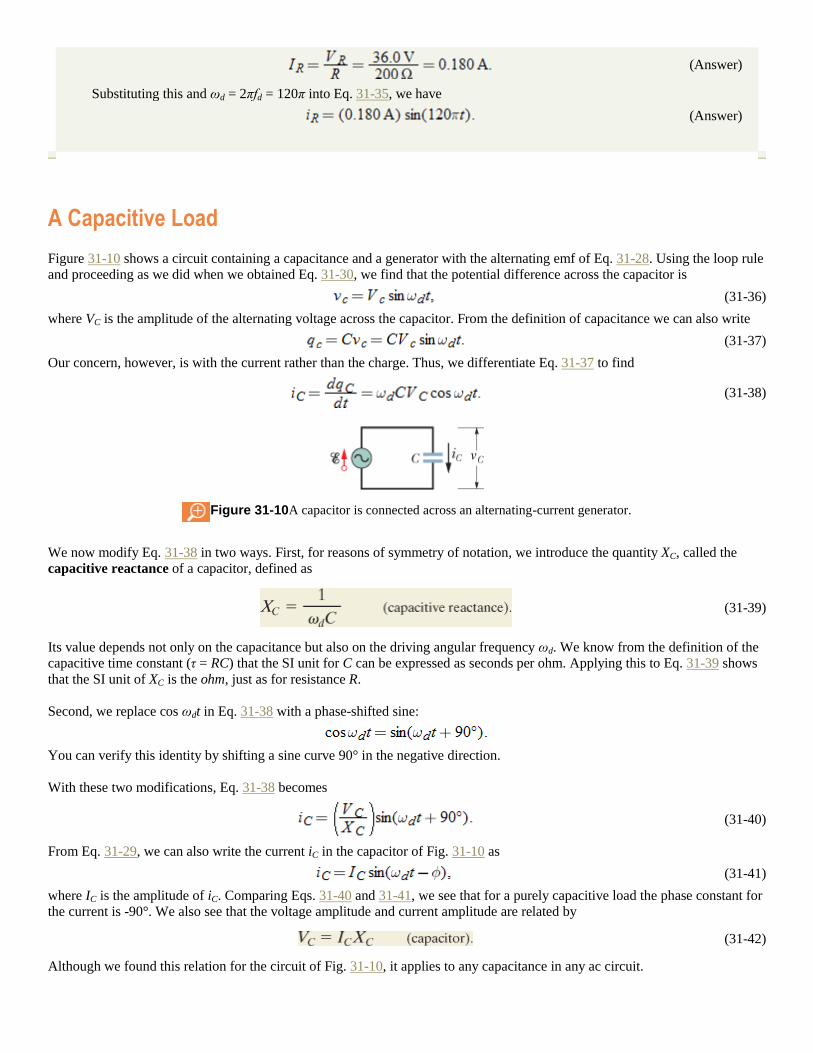
A Capacitive Load

Figure 31-10 shows a circuit containing a capacitance and a generator with the alternating emf of Eq. 31-28. Using the loop rule

and proceeding as we did when we obtained Eq. 31-30, we find that the potential difference across the capacitor is

(31-36)

where VC is the amplitude of the alternating voltage across the capacitor. From the definition of capacitance we can also write

(31-37)

Our concern, however, is with the current rather than the charge. Thus, we differentiate Eq. 31-37 to find

(31-38)

Figure 31-10 A capacitor is connected across an alternating-current generator.

We now modify Eq. 31-38 in two ways. First, for reasons of symmetry of notation, we introduce the quantity XC, called the

capacitive reactance of a capacitor, defined as

(31-39)

Its value depends not only on the capacitance but also on the driving angular frequency ωd. We know from the definition of the

capacitive time constant (τ = RC) that the SI unit for C can be expressed as seconds per ohm. Applying this to Eq. 31-39 shows

that the SI unit of XC is the ohm, just as for resistance R.

Second, we replace cos ωdt in Eq. 31-38 with a phase-shifted sine:

You can verify this identity by shifting a sine curve 90° in the negative direction.

With these two modifications, Eq. 31-38 becomes

(31-40)

From Eq. 31-29, we can also write the current iC in the capacitor of Fig. 31-10 as

(31-41)

where IC is the amplitude of iC. Comparing Eqs. 31-40 and 31-41, we see that for a purely capacitive load the phase constant for

the current is -90°. We also see that the voltage amplitude and current amplitude are related by

(31-42)

Although we found this relation for the circuit of Fig. 31-10, it applies to any capacitance in any ac circuit.

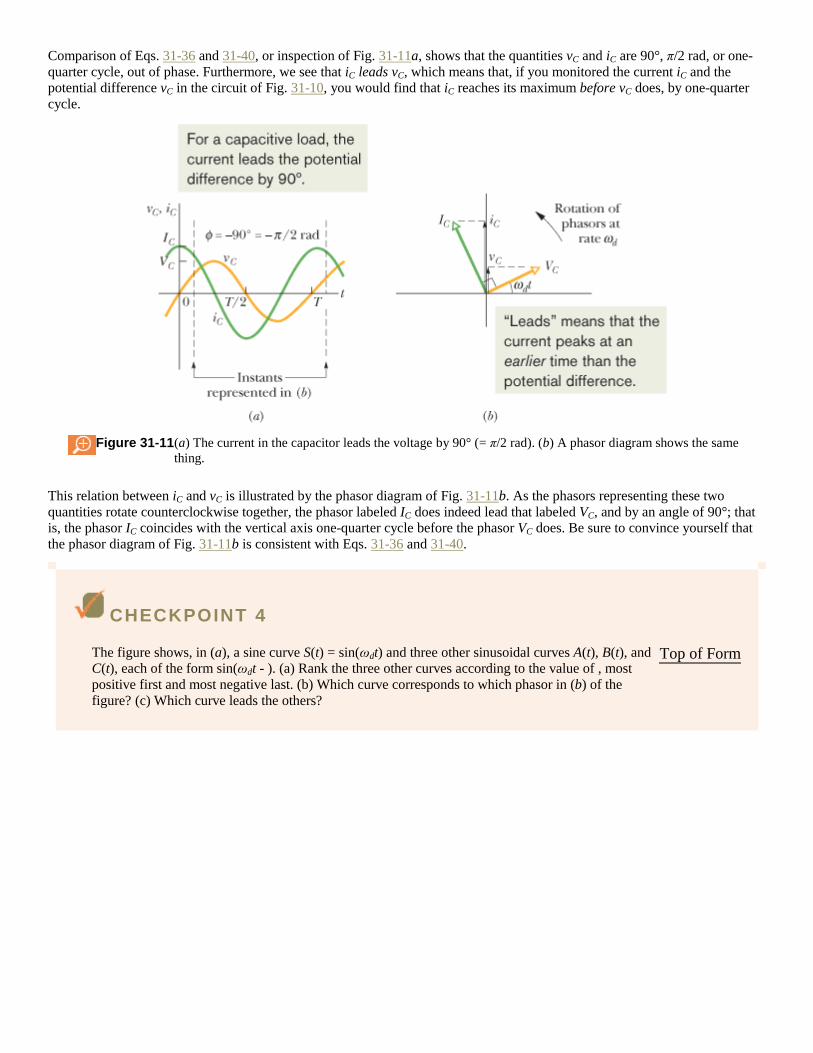
Comparison of Eqs. 31-36 and 31-40, or inspection of Fig. 31-11a, shows that the quantities vC and iC are 90°, π/2 rad, or one-

quarter cycle, out of phase. Furthermore, we see that iC leads vC, which means that, if you monitored the current iC and the

potential difference vC in the circuit of Fig. 31-10, you would find that iC reaches its maximum before vC does, by one-quarter

cycle.

Figure 31-11 (a) The current in the capacitor leads the voltage by 90° (= π/2 rad). (b) A phasor diagram shows the same

thing.

This relation between iC and vC is illustrated by the phasor diagram of Fig. 31-11b. As the phasors representing these two

quantities rotate counterclockwise together, the phasor labeled IC does indeed lead that labeled VC, and by an angle of 90°; that

is, the phasor IC coincides with the vertical axis one-quarter cycle before the phasor VC does. Be sure to convince yourself that

the phasor diagram of Fig. 31-11b is consistent with Eqs. 31-36 and 31-40.

CHECKPOINT 4

The figure shows, in (a), a sine curve S(t) = sin(ωdt) and three other sinusoidal curves A(t), B(t), and

C(t), each of the form sin(ωdt - ). (a) Rank the three other curves according to the value of , most

positive first and most negative last. (b) Which curve corresponds to which phasor in (b) of the

figure? (c) Which curve leads the others?

Top of Form

Sample Problem

Purely capacitive load: potential difference and current

In Fig. 31-10, capacitance C is 15.0 μF and the sinusoidal alternating emf device operates at amplitude m = 36.0 V

and frequency fd = 60.0 Hz.

(a) What are the potential difference vC(t) across the capacitance and the amplitude VC of vC(t)?

KEY IDEA

In a circuit with a purely capacitive load, the potential difference vC(t) across the capacitance is always equal to the

potential difference (t) across the emf device.

Calculations:

Here we have vC(t) = (t) and VC = m. Since m is given, we have

(Answer)

To find vC(t), we use Eq. 31-28 to write

(31-43)

Then, substituting m = 36.0 V and ωd = 2πfd = 120π into Eq. 31-43, we have

(Answer)

(b) What are the current iC(t) in the circuit as a function of time and the amplitude IC of iC(t)?

KEY IDEA

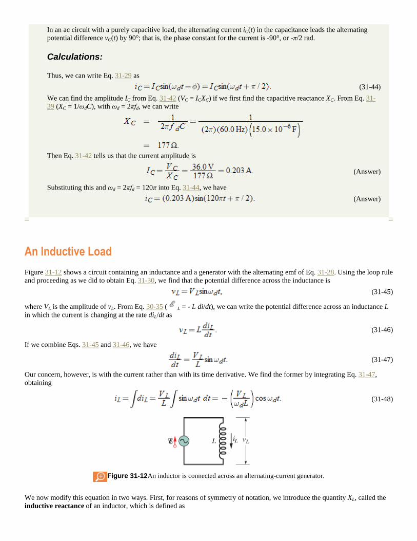
In an ac circuit with a purely capacitive load, the alternating current iC(t) in the capacitance leads the alternating

potential difference vC(t) by 90°; that is, the phase constant for the current is -90°, or -π/2 rad.

Calculations:

Thus, we can write Eq. 31-29 as

(31-44)

We can find the amplitude IC from Eq. 31-42 (VC = ICXC) if we first find the capacitive reactance XC. From Eq. 31-

39 (XC = 1/ωdC), with ωd = 2πfd, we can write

Then Eq. 31-42 tells us that the current amplitude is

(Answer)

Substituting this and ωd = 2πfd = 120π into Eq. 31-44, we have

(Answer)

An Inductive Load

Figure 31-12 shows a circuit containing an inductance and a generator with the alternating emf of Eq. 31-28. Using the loop rule

and proceeding as we did to obtain Eq. 31-30, we find that the potential difference across the inductance is

(31-45)

where VL is the amplitude of vL. From Eq. 30-35 ( L = - L di/dt), we can write the potential difference across an inductance L

in which the current is changing at the rate diL/dt as

(31-46)

If we combine Eqs. 31-45 and 31-46, we have

(31-47)

Our concern, however, is with the current rather than with its time derivative. We find the former by integrating Eq. 31-47,

obtaining

(31-48)

Figure 31-12 An inductor is connected across an alternating-current generator.

We now modify this equation in two ways. First, for reasons of symmetry of notation, we introduce the quantity XL, called the

inductive reactance of an inductor, which is defined as

(31-49)

The value of XL depends on the driving angular frequency ωd. The unit of the inductive time constant τL indicates that the SI unit

of XL is the ohm, just as it is for XC and for R.

Second, we replace -cos ωdt in Eq. 31-48 with a phase-shifted sine:

You can verify this identity by shifting a sine curve 90° in the positive direction.

With these two changes, Eq. 31-48 becomes

(31-50)

From Eq. 31-29, we can also write this current in the inductance as

(31-51)

where IL is the amplitude of the current iL. Comparing Eqs. 31-50 and 31-51, we see that for a purely inductive load the phase

constant for the current is +90°. We also see that the voltage amplitude and current amplitude are related by

(31-52)

Although we found this relation for the circuit of Fig. 31-12, it applies to any inductance in any ac circuit.

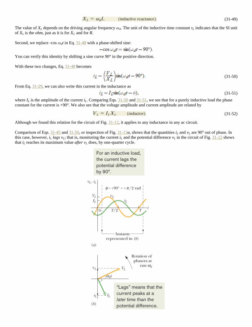
Comparison of Eqs. 31-45 and 31-50, or inspection of Fig. 31-13a, shows that the quantities iL and vL are 90° out of phase. In

this case, however, iL lags vL; that is, monitoring the current iL and the potential difference vL in the circuit of Fig. 31-12 shows

that iL reaches its maximum value after vL does, by one-quarter cycle.

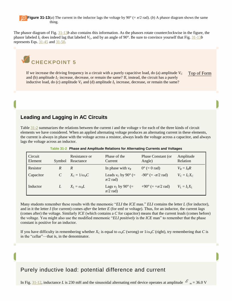
Figure 31-13 (a) The current in the inductor lags the voltage by 90° (= π/2 rad). (b) A phasor diagram shows the same

thing.

The phasor diagram of Fig. 31-13b also contains this information. As the phasors rotate counterclockwise in the figure, the

phasor labeled IL does indeed lag that labeled VL, and by an angle of 90°. Be sure to convince yourself that Fig. 31-13b

represents Eqs. 31-45 and 31-50.

CHECKPOINT 5

If we increase the driving frequency in a circuit with a purely capacitive load, do (a) amplitude VC

and (b) amplitude IC increase, decrease, or remain the same? If, instead, the circuit has a purely

inductive load, do (c) amplitude VL and (d) amplitude IL increase, decrease, or remain the same?

Top of Form

Problem-Solving Tactics

Leading and Lagging in AC Circuits

Table 31-2 summarizes the relations between the current i and the voltage v for each of the three kinds of circuit

elements we have considered. When an applied alternating voltage produces an alternating current in these elements,

the current is always in phase with the voltage across a resistor, always leads the voltage across a capacitor, and always

lags the voltage across an inductor.

Table 31-2 Phase and Amplitude Relations for Alternating Currents and Voltages

Circuit

Element Symbol

Resistance or

Reactance

Phase of the

Current

Phase Constant (or

Angle)

Amplitude

Relation

Resistor R R In phase with vR 0° (= 0 rad) VR = IRR

Capacitor C XC = 1/ωdC Leads vC by 90° (=

π/2 rad)

-90° (= -π/2 rad) VC = ICXC

Inductor L XL = ωdL Lags vL by 90° (=

π/2 rad)

+90° (= +π/2 rad) VL = ILXL

Many students remember these results with the mnemonic “ELI the ICE man.” ELI contains the letter L (for inductor),

and in it the letter I (for current) comes after the letter E (for emf or voltage). Thus, for an inductor, the current lags

(comes after) the voltage. Similarly ICE (which contains a C for capacitor) means that the current leads (comes before)

the voltage. You might also use the modified mnemonic “ELI positively is the ICE man” to remember that the phase

constant is positive for an inductor.

If you have difficulty in remembering whether XC is equal to ωdC (wrong) or 1/ωdC (right), try remembering that C is

in the “cellar”—that is, in the denominator.

Sample Problem

Purely inductive load: potential difference and current

In Fig. 31-12, inductance L is 230 mH and the sinusoidal alternating emf device operates at amplitude m = 36.0 V

and frequency fd = 60.0 Hz.

(a) What are the potential difference vL(t) across the inductance and the amplitude VL of vL(t)?

KEY IDEA

In a circuit with a purely inductive load, the potential difference vL(t) across the inductance is always equal to the

potential difference (t) across the emf device.

Calculations:

Here we have vL(t) = (t) and VL = m. Since m is given, we know that

(Answer)

To find vL(t), we use Eq. 31-28 to write

(31-53)

Then, substituting m = 36.0 V and ωd = 2πfd = 120π into Eq. 31-53, we have

(Answer)

(b) What are the current iL(t) in the circuit as a function of time and the amplitude IL of iL(t)?

KEY IDEA

In an ac circuit with a purely inductive load, the alternating current iL(t) in the inductance lags the alternating

potential difference vL(t) by 90°. (In the mnemonic of the problem-solving tactic, this circuit is “positively an ELI

circuit,” which tells us that the emf E leads the current I and that is positive.)

Calculations:

Because the phase constant for the current is +90°, or +π/2 rad, we can write Eq. 31-29 as

(31-54)

We can find the amplitude IL from Eq. 31-52 (VL = ILXL) if we first find the inductive reactance XL. From Eq. 31-49

(XL = ωdL), with ωd = 2πfd, we can write

Then Eq. 31-52 tells us that the current amplitude is

(Answer)

Substituting this and ωd = 2πfd = 120π into Eq. 31-54, we have

(Answer)

Copyright © 2011 John Wiley & Sons, Inc. All rights reserved.

31-9 The Series RLC Circuit

We are now ready to apply the alternating emf of Eq. 31-28,

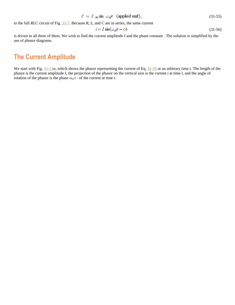
(31-55)

to the full RLC circuit of Fig. 31-7. Because R, L, and C are in series, the same current

(31-56)

is driven in all three of them. We wish to find the current amplitude I and the phase constant . The solution is simplified by the

use of phasor diagrams.

The Current Amplitude

We start with Fig. 31-14a, which shows the phasor representing the current of Eq. 31-56 at an arbitrary time t. The length of the

phasor is the current amplitude I, the projection of the phasor on the vertical axis is the current i at time t, and the angle of

rotation of the phasor is the phase ωd t - of the current at time t.

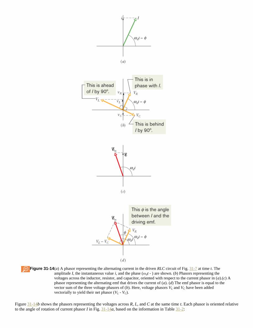
Figure 31-14 (a) A phasor representing the alternating current in the driven RLC circuit of Fig. 31-7 at time t. The

amplitude I, the instantaneous value i, and the phase (ωdt - ) are shown. (b) Phasors representing the

voltages across the inductor, resistor, and capacitor, oriented with respect to the current phasor in (a).(c) A

phasor representing the alternating emf that drives the current of (a). (d) The emf phasor is equal to the

vector sum of the three voltage phasors of (b). Here, voltage phasors VL and VC have been added

vectorially to yield their net phasor (VL - VC).

Figure 31-14b shows the phasors representing the voltages across R, L, and C at the same time t. Each phasor is oriented relative

to the angle of rotation of current phasor I in Fig. 31-14a, based on the information in Table 31-2:

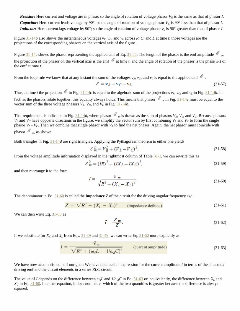
Resistor: Here current and voltage are in phase; so the angle of rotation of voltage phasor VR is the same as that of phasor I.

Capacitor: Here current leads voltage by 90°; so the angle of rotation of voltage phasor VC is 90° less than that of phasor I.

Inductor: Here current lags voltage by 90°; so the angle of rotation of voltage phasor vL is 90° greater than that of phasor I.

Figure 31-14b also shows the instantaneous voltages vR, vC, and vL across R, C, and L at time t; those voltages are the

projections of the corresponding phasors on the vertical axis of the figure.

Figure 31-14c shows the phasor representing the applied emf of Eq. 31-55. The length of the phasor is the emf amplitude m,

the projection of the phasor on the vertical axis is the emf at time t, and the angle of rotation of the phasor is the phase ωdt of

the emf at time t.

From the loop rule we know that at any instant the sum of the voltages vR, vC, and vL is equal to the applied emf :

(31-57)

Thus, at time t the projection in Fig. 31-14c is equal to the algebraic sum of the projections vR, vC, and vL in Fig. 31-14b. In

fact, as the phasors rotate together, this equality always holds. This means that phasor m in Fig. 31-14c must be equal to the

vector sum of the three voltage phasors VR, VC, and VL in Fig. 31-14b.

That requirement is indicated in Fig. 31-14d, where phasor m is drawn as the sum of phasors VR, VL, and VC. Because phasors

VL and VC have opposite directions in the figure, we simplify the vector sum by first combining VL and VC to form the single

phasor VL - VC. Then we combine that single phasor with VR to find the net phasor. Again, the net phasor must coincide with

phasor m, as shown.

Both triangles in Fig. 31-14d are right triangles. Applying the Pythagorean theorem to either one yields

(31-58)

From the voltage amplitude information displayed in the rightmost column of Table 31-2, we can rewrite this as

(31-59)

and then rearrange it to the form

(31-60)

The denominator in Eq. 31-60 is called the impedance Z of the circuit for the driving angular frequency ωd:

(31-61)

We can then write Eq. 31-60 as

(31-62)

If we substitute for XC and XL from Eqs. 31-39 and 31-49, we can write Eq. 31-60 more explicitly as

(31-63)

We have now accomplished half our goal: We have obtained an expression for the current amplitude I in terms of the sinusoidal

driving emf and the circuit elements in a series RLC circuit.

The value of I depends on the difference between ωdL and 1/ωdC in Eq. 31-63 or, equivalently, the difference between XL and

XC in Eq. 31-60. In either equation, it does not matter which of the two quantities is greater because the difference is always

squared.

The current that we have been describing in this section is the steady-state current that occurs after the alternating emf has been

applied for some time. When the emf is first applied to a circuit, a brief transient current occurs. Its duration (before settling

down into the steady-state current) is determined by the time constants τL = L/R and τC = RC as the inductive and capacitive

elements “turn on.” This transient current can, for example, destroy a motor on start-up if it is not properly taken into account in

the motor's circuit design.

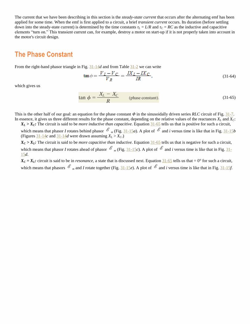
The Phase Constant

From the right-hand phasor triangle in Fig. 31-14d and from Table 31-2 we can write

(31-64)

which gives us

(31-65)

This is the other half of our goal: an equation for the phase constant Φ in the sinusoidally driven series RLC circuit of Fig. 31-7.

In essence, it gives us three different results for the phase constant, depending on the relative values of the reactances XL and XC:

XL > XC: The circuit is said to be more inductive than capacitive. Equation 31-65 tells us that is positive for such a circuit,

which means that phasor I rotates behind phasor m (Fig. 31-15a). A plot of and i versus time is like that in Fig. 31-15b

(Figures 31-14c and 31-14d were drawn assuming XL > XC.)

XC > XL: The circuit is said to be more capacitive than inductive. Equation 31-65 tells us that is negative for such a circuit,

which means that phasor I rotates ahead of phasor m (Fig. 31-15c). A plot of and i versus time is like that in Fig. 31-

15d.

XC = XL: circuit is said to be in resonance, a state that is discussed next. Equation 31-65 tells us that = 0° for such a circuit,

which means that phasors m and I rotate together (Fig. 31-15e). A plot of and i versus time is like that in Fig. 31-15f.

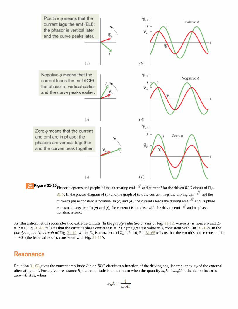
Figure 31-15 Phasor diagrams and graphs of the alternating emf and current i for the driven RLC circuit of Fig.

31-7. In the phasor diagram of (a) and the graph of (b), the current i lags the driving emf and the

current's phase constant is positive. In (c) and (d), the current i leads the driving emf and its phase

constant is negative. In (e) and (f), the current i is in phase with the driving emf and its phase

constant is zero.

As illustration, let us reconsider two extreme circuits: In the purely inductive circuit of Fig. 31-12, where XL is nonzero and XC

= R = 0, Eq. 31-65 tells us that the circuit's phase constant is = +90° (the greatest value of ), consistent with Fig. 31-13b. In the

purely capacitive circuit of Fig. 31-10, where XC is nonzero and XL = R = 0, Eq. 31-65 tells us that the circuit's phase constant is

= -90° (the least value of ), consistent with Fig. 31-11b.

Resonance

Equation 31-63 gives the current amplitude I in an RLC circuit as a function of the driving angular frequency ωd of the external

alternating emf. For a given resistance R, that amplitude is a maximum when the quantity ωdL - 1/ωdC in the denominator is

zero—that is, when

or

(31-66)

Because the natural angular frequency ω of the RLC circuit is also equal to , the maximum value of I occurs when the

driving angular frequency matches the natural angular frequency—that is, at resonance. Thus, in an RLC circuit, resonance and

maximum current amplitude I occur when

(31-67)

Figure 31-16 shows three resonance curves for sinusoidally driven oscillations in three series RLC circuits differing only in R.

Each curve peaks at its maximum current amplitude I when the ratio ωd/ω is 1.00, but the maximum value of I decreases with

increasing R. (The maximum I is always m/R; to see why, combine Eqs. 31-61 and 31-62.) In addition, the curves increase in

width (measured in Fig. 31-16 at half the maximum value of I) with increasing R.

Current Amplitude Versus Angular Frequencies

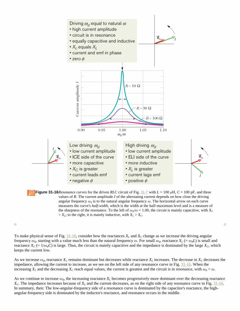
Figure 31-16 Resonance curves for the driven RLC circuit of Fig. 31-7 with L = 100 μH, C = 100 pF, and three

values of R. The current amplitude I of the alternating current depends on how close the driving

angular frequency ωd is to the natural angular frequency ω. The horizontal arrow on each curve

measures the curve's half-width, which is the width at the half-maximum level and is a measure of

the sharpness of the resonance. To the left of ωd/ω = 1.00, the circuit is mainly capacitive, with XC

> XL; to the right, it is mainly inductive, with XL > XC.

To make physical sense of Fig. 31-16, consider how the reactances XL and XC change as we increase the driving angular

frequency ωd, starting with a value much less than the natural frequency ω. For small ωd, reactance XL (= ωdL) is small and

reactance XC (= 1/ωdC) is large. Thus, the circuit is mainly capacitive and the impedance is dominated by the large XC, which

keeps the current low.

As we increase ωd, reactance XC remains dominant but decreases while reactance XL increases. The decrease in XC decreases the

impedance, allowing the current to increase, as we see on the left side of any resonance curve in Fig. 31-16. When the

increasing XL and the decreasing XC reach equal values, the current is greatest and the circuit is in resonance, with ωd = ω.

As we continue to increase ωd, the increasing reactance XL becomes progressively more dominant over the decreasing reactance

XC. The impedance increases because of XL and the current decreases, as on the right side of any resonance curve in Fig. 31-16.

In summary, then: The low-angular-frequency side of a resonance curve is dominated by the capacitor's reactance, the high-

angular-frequency side is dominated by the inductor's reactance, and resonance occurs in the middle.

CHECKPOINT 6

Here are the capacitive reactance and inductive reactance, respectively, for three sinusoidally driven

series RLC circuits: (1) 50 Ω, 100 Ω; (2) 100 Ω, 50 Ω; (3) 50 Ω, 50 Ω. (a) For each, does the current

lead or lag the applied emf, or are the two in phase? (b) Which circuit is in resonance?

Top of Form

Sample Problem

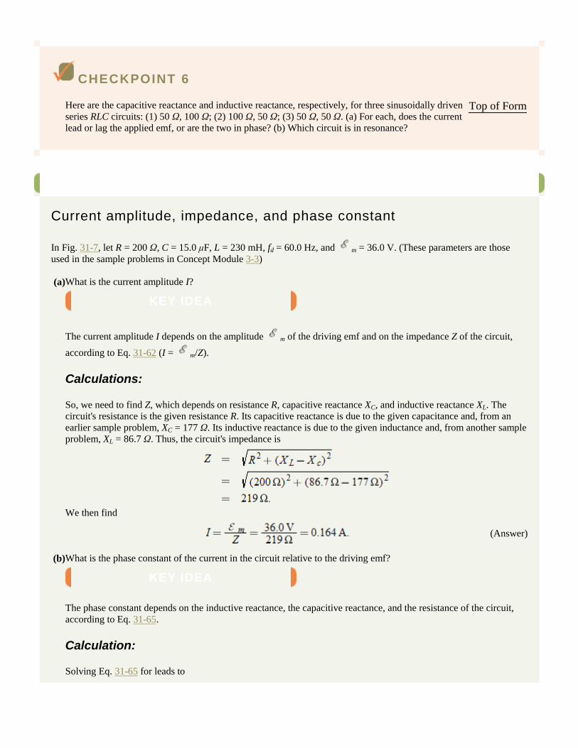
Current amplitude, impedance, and phase constant

In Fig. 31-7, let R = 200 Ω, C = 15.0 μF, L = 230 mH, fd = 60.0 Hz, and m = 36.0 V. (These parameters are those

used in the sample problems in Concept Module 3-3)

(a) What is the current amplitude I?

KEY IDEA

The current amplitude I depends on the amplitude m of the driving emf and on the impedance Z of the circuit,

according to Eq. 31-62 (I = m/Z).

Calculations:

So, we need to find Z, which depends on resistance R, capacitive reactance XC, and inductive reactance XL. The

circuit's resistance is the given resistance R. Its capacitive reactance is due to the given capacitance and, from an

earlier sample problem, XC = 177 Ω. Its inductive reactance is due to the given inductance and, from another sample

problem, XL = 86.7 Ω. Thus, the circuit's impedance is

We then find

(Answer)

(b) What is the phase constant of the current in the circuit relative to the driving emf?

KEY IDEA

The phase constant depends on the inductive reactance, the capacitive reactance, and the resistance of the circuit,

according to Eq. 31-65.

Calculation:

Solving Eq. 31-65 for leads to

(Answer)

The negative phase constant is consistent with the fact that the load is mainly capacitive; that is, XC > XL. In the

common mnemonic for driven series RLC circuits, this circuit is an ICE circuit—the current leads the driving emf.

Copyright © 2011 John Wiley & Sons, Inc. All rights reserved.

31-10 Power in Alternating-Current Circuits

In the RLC circuit of Fig. 31-7, the source of energy is the alternating-current generator. Some of the energy that it provides is

stored in the electric field in the capacitor, some is stored in the magnetic field in the inductor, and some is dissipated as thermal

energy in the resistor. In steady-state operation, the average stored energy remains constant. The net transfer of energy is thus

from the generator to the resistor, where energy is dissipated.

The instantaneous rate at which energy is dissipated in the resistor can be written, with the help of Eqs. 26-27 and 31-29, as

(31-68)

The average rate at which energy is dissipated in the resistor, however, is the average of Eq. 31-68 over time. Over one

complete cycle, the average value of sin θ, where θ is any variable, is zero (Fig. 31-17a) but the average value of sin2 θ is

(Fig. 31-17b). (Note in Fig. 31-17b how the shaded areas under the curve but above the horizontal line marked exactly fill

in the unshaded spaces below that line.) Thus, we can write, from Eq. 31-68,

(31-69)

The quantity is called the root-mean-square, or rms, value of the current i:

(31-70)

We can now rewrite Eq. 31-69 as

(31-71)

Equation 31-71 looks much like Eq. 26-27 (P = i2R); the message is that if we switch to the rms current, we can compute the

average rate of energy dissipation for alternating-current circuits just as for direct-current circuits.

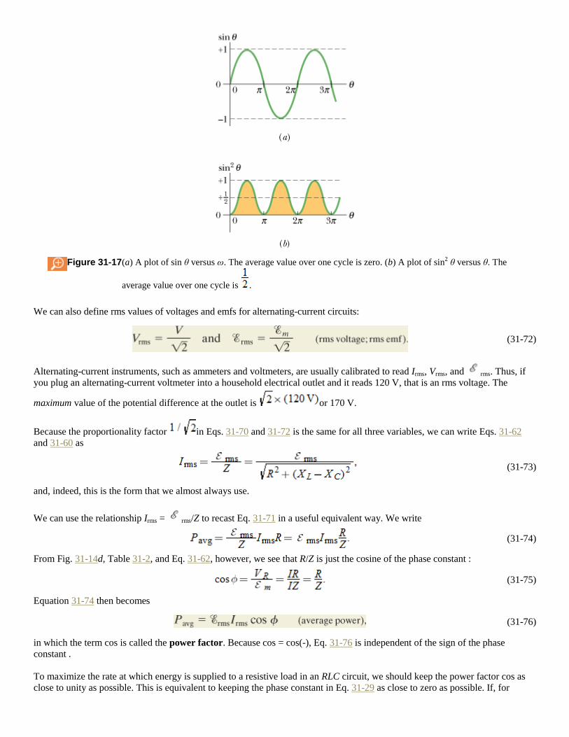
Figure 31-17 (a) A plot of sin θ versus ω. The average value over one cycle is zero. (b) A plot of sin2 θ versus θ. The

average value over one cycle is .

We can also define rms values of voltages and emfs for alternating-current circuits:

(31-72)

Alternating-current instruments, such as ammeters and voltmeters, are usually calibrated to read Irms, Vrms, and rms. Thus, if

you plug an alternating-current voltmeter into a household electrical outlet and it reads 120 V, that is an rms voltage. The

maximum value of the potential difference at the outlet is or 170 V.

Because the proportionality factor in Eqs. 31-70 and 31-72 is the same for all three variables, we can write Eqs. 31-62

and 31-60 as

(31-73)

and, indeed, this is the form that we almost always use.

We can use the relationship Irms = rms/Z to recast Eq. 31-71 in a useful equivalent way. We write

(31-74)

From Fig. 31-14d, Table 31-2, and Eq. 31-62, however, we see that R/Z is just the cosine of the phase constant :

(31-75)

Equation 31-74 then becomes

(31-76)

in which the term cos is called the power factor. Because cos = cos(-), Eq. 31-76 is independent of the sign of the phase

constant .

To maximize the rate at which energy is supplied to a resistive load in an RLC circuit, we should keep the power factor cos as

close to unity as possible. This is equivalent to keeping the phase constant in Eq. 31-29 as close to zero as possible. If, for

example, the circuit is highly inductive, it can be made less so by putting more capacitance in the circuit, connected in series.

(Recall that putting an additional capacitance into a series of capacitances decreases the equivalent capacitance Ceq of the

series.) Thus, the resulting decrease in Ceq in the circuit reduces the phase constant and increases the power factor in Eq. 31-76.

Power companies place series-connected capacitors throughout their transmission systems to get these results.

CHECKPOINT 7

(a) If the current in a sinusoidally driven series RLC circuit leads the emf, would we increase or

decrease the capacitance to increase the rate at which energy is supplied to the resistance? (b) Would

this change bring the resonant angular frequency of the circuit closer to the angular frequency of the

emf or put it farther away?

Top of Form

Sample Problem

Driven RLC circuit: power factor and average power

A series RLC circuit, driven with rms = 120 V at frequency fd = 60.0 Hz, contains a resistance R = 200 Ω, an

inductance with inductive reactance XL = 80.0 Ω, and a capacitance with capacitive reactance XC = 150 Ω.

(a) What are the power factor cos and phase constant of the circuit?

KEY IDEA

The power factor cos can be found from the resistance R and impedance Z via Eq. 31-75 (cos = R/Z).

Calculations:

To calculate Z, we use Eq. 31-61:

Equation 31-75 then gives us

(Answer)

Taking the inverse cosine then yields

Both +19.3° and -19.3° have a cosine of 0.944. To determine which sign is correct, we must consider whether the

current leads or lags the driving emf. Because XC > XL, this circuit is mainly capacitive, with the current leading the

emf. Thus, must be negative:

(Answer)

We could, instead, have found with Eq. 31-65. A calculator would then have given us the answer with the minus

sign.

(b) What is the average rate Pavg at which energy is dissipated in the resistance?

KEY IDEAS

There are two ways and two ideas to use: (1) Because the circuit is assumed to be in steady-state operation, the rate

at which energy is dissipated in the resistance is equal to the rate at which energy is supplied to the circuit, as given

by Eq. 31-76 (Pavg = rmsIrms cos ). (2) The rate at which energy is dissipated in a resistance R depends on the

square of the rms current Irms through it, according to Eq. 31-71 (Pavg = I2

rms R).

First way:

We are given the rms driving emf rms and we already know cos from part (a). The rms current Irms is determined

by the rms value of the driving emf and the circuit's impedance Z (which we know), according to Eq. 31-73:

Substituting this into Eq. 31-76 then leads to

(Answer)

Second way: Instead, we can write

(Answer)

(c) What new capacitance Cnew is needed to maximize Pavg if the other parameters of the circuit are not changed?

KEY IDEAS

(1) The average rate Pavg at which energy is supplied and dissipated is maximized if the circuit is brought into

resonance with the driving emf. (2) Resonance occurs when XC = XL.

Calculations:

From the given data, we have XC > XL. Thus, we must decrease XC to reach resonance. From Eq. 31-39 (XC =

1/ωdC), we see that this means we must increase C to the new value Cnew.

Using Eq. 31-39, we can write the resonance condition XC = XL as

Substituting 2πfd for ωd (because we are given fd and not ωd) and then solving for Cnew, we find

(Answer)

Following the procedure of part (b), you can show that with Cnew, the average power of energy dissipation Pavg

would then be at its maximum value of

Copyright © 2011 John Wiley & Sons, Inc. All rights reserved.

31-11 Transformers

Energy Transmission Requirements

When an ac circuit has only a resistive load, the power factor in Eq. 31-76 is cos 0° = 1 and the applied rms emf rms is equal

to the rms voltage Vrms across the load. Thus, with an rms current Irms in the load, energy is supplied and dissipated at the

average rate of

(31-77)

(In Eq. 31-77 and the rest of this section, we follow conventional practice and drop the subscripts identifying rms quantities.

Engineers and scientists assume that all time-varying currents and voltages are reported as rms values; that is what the meters

read.) Equation 31-77 tells us that, to satisfy a given power requirement, we have a range of choices for I and V, provided only

that the product IV is as required.

In electrical power distribution systems it is desirable for reasons of safety and for efficient equipment design to deal with

relatively low voltages at both the generating end (the electrical power plant) and the receiving end (the home or factory).

Nobody wants an electric toaster or a child's electric train to operate at, say, 10 kV. On the other hand, in the transmission of

electrical energy from the generating plant to the consumer, we want the lowest practical current (hence the largest practical

voltage) to minimize I2R losses (often called ohmic losses) in the transmission line.

As an example, consider the 735 kV line used to transmit electrical energy from the La Grande 2 hydroelectric plant in Quebec

to Montreal, 1000 km away. Suppose that the current is 500 A and the power factor is close to unity. Then from Eq. 31-77,

energy is supplied at the average rate

The resistance of the transmission line is about 0.220 Ω/km; thus, there is a total resistance of about 220 Ω for the 1000 km

stretch. Energy is dissipated due to that resistance at a rate of about

which is nearly 15% of the supply rate.

Imagine what would happen if we doubled the current and halved the voltage. Energy would be supplied by the plant at the

same average rate of 368 MW as previously, but now energy would be dissipated at the rate of about

which is almost 60% of the supply rate. Hence the general energy transmission rule: Transmit at the highest possible voltage

and the lowest possible current.

The Ideal Transformer

The transmission rule leads to a fundamental mismatch between the requirement for efficient high-voltage transmission and the

need for safe low-voltage generation and consumption. We need a device with which we can raise (for transmission) and lower

(for use) the ac voltage in a circuit, keeping the product current × voltage essentially constant. The transformer is such a

device. It has no moving parts, operates by Faraday's law of induction, and has no simple direct-current counterpart.

The ideal transformer in Fig. 31-18 consists of two coils, with different numbers of turns, wound around an iron core. (The

coils are insulated from the core.) In use, the primary winding, of Np turns, is connected to an alternating-current generator

whose emf at any time t is given by

(31-78)

The secondary winding, of Ns turns, is connected to load resistance R, but its circuit is an open circuit as long as switch S is

open (which we assume for the present). Thus, there can be no current through the secondary coil. We assume further for this

ideal transformer that the resistances of the primary and secondary windings are negligible. Well-designed, high-capacity

transformers can have energy losses as low as 1%; so our assumptions are reasonable.

Figure 31-18 An ideal transformer (two coils wound on an iron core) in a basic transformer circuit. An ac generator

produces current in the coil at the left (the primary). The coil at the right (the secondary) is connected to

the resistive load R when switch S is closed.

For the assumed conditions, the primary winding (or primary) is a pure inductance and the primary circuit is like that in Fig. 31-

12. Thus, the (very small) primary current, also called the magnetizing current Imag, lags the primary voltage Vp by 90°; the

primary's power factor (= cos in Eq. 31-76) is zero; so no power is delivered from the generator to the transformer.

However, the small sinusoidally changing primary current Imag produces a sinusoidally changing magnetic flux ΦB in the iron

core. The core acts to strengthen the flux and to bring it through the secondary winding (or secondary). Because ΦB varies, it

induces an emf turn (= dΦB/dt) in each turn of the secondary. In fact, this emf per turn turn is the same in the primary and

the secondary. Across the primary, the voltage Vp is the product of turn and the number of turns Np; that is, Vp = turnNp.

Similarly, across the secondary the voltage is Vs = turnNs. Thus, we can write

or

(31-79)

If Ns > Np, the device is a step-up transformer because it steps the primary's voltage Vp up to a higher voltage Vs. Similarly, if Ns

< Np, it is a step-down transformer.

With switch S open, no energy is transferred from the generator to the rest of the circuit, but when we close S to connect the

secondary to the resistive load R, energy is transferred. (In general, the load would also contain inductive and capacitive

elements, but here we consider just resistance R.) Here is the process:

1.

An alternating current Is appears in the secondary circuit, with corresponding energy dissipation rate in

the resistive load.

2. This current produces its own alternating magnetic flux in the iron core, and this flux induces an opposing emf in the

primary windings.

3. The voltage Vp of the primary, however, cannot change in response to this opposing emf because it must always be equal

to the emf that is provided by the generator; closing switch S cannot change this fact.

4. To maintain Vp, the generator now produces (in addition to Imag) an alternating current Ip in the primary circuit; the

magnitude and phase constant of Ip are just those required for the emf induced by Ip in the primary to exactly cancel the

emf induced there by Is. Because the phase constant of Ip is not 90° like that of Imag, this current Ip can transfer energy to

the primary.

We want to relate Is to Ip. However, rather than analyze the foregoing complex process in detail, let us just apply the principle of

conservation of energy. The rate at which the generator transfers energy to the primary is equal to IpVp. The rate at which the

primary then transfers energy to the secondary (via the alternating magnetic field linking the two coils) is IsVs. Because we

assume that no energy is lost along the way, conservation of energy requires that

Substituting for Vs from Eq. 31-79, we find that

(31-80)

This equation tells us that the current Is in the secondary can differ from the current Ip in the primary, depending on the turns ratio Np/Ns.

Current Ip appears in the primary circuit because of the resistive load R in the secondary circuit. To find Ip, we substitute Is =

Vs/R into Eq. 31-80 and then we substitute for Vs from Eq. 31-79. We find

(31-81)

This equation has the form Ip = Vp/Req, where equivalent resistance Req is

(31-82)

This Req is the value of the load resistance as “seen” by the generator; the generator produces the current Ip and voltage Vp as if

the generator were connected to a resistance Req.

Impedance Matching

Equation 31-82 suggests still another function for the transformer. For maximum transfer of energy from an emf device to a

resistive load, the resistance of the emf device must equal the resistance of the load. The same relation holds for ac circuits

except that the impedance (rather than just the resistance) of the generator must equal that of the load. Often this condition is not

met. For example, in a music-playing system, the amplifier has high impedance and the speaker set has low impedance. We can

match the impedances of the two devices by coupling them through a transformer that has a suitable turns ratio Np/Ns.

CHECKPOINT 8

An alternating-current emf device in a certain circuit has a smaller resistance than that of the

resistive load in the circuit; to increase the transfer of energy from the device to the load, a

transformer will be connected between the two. (a) Should Ns be greater than or less than Np? (b)

Will that make it a step-up or step-down transformer?

Top of Form

Sample Problem

Transformer: turns ratio, average power, rms currents

A transformer on a utility pole operates at Vp = 8.5 kV on the primary side and supplies electrical energy to a number of

nearby houses at Vs = 120 V, both quantities being rms values. Assume an ideal step-down transformer, a purely

resistive load, and a power factor of unity.

(a) What is the turns ratio Np/Ns of the transformer?

KEY IDEA

The turns ratio Np/Ns is related to the (given) rms primary and secondary voltages via Eq. 31-79 (Vs = VpNs/Np).

Calculation:

We can write Eq. 31-79 as

(31-83)

(Note that the right side of this equation is the inverse of the turns ratio.) Inverting both sides of Eq. 31-83 gives us

(Answer)

(b) The average rate of energy consumption (or dissipation) in the houses served by the transformer is 78 kW. What are

the rms currents in the primary and secondary of the transformer?

KEY IDEA

For a purely resistive load, the power factor cos is unity; thus, the average rate at which energy is supplied and

dissipated is given by Eq. 31-77 (Pavg = I = IV).

Calculations:

In the primary circuit, with Vp = 8.5 kV, Eq. 31-77 yields

(Answer)

Similarly, in the secondary circuit,

(Answer)

You can check that Is = Ip(Np/Ns) as required by Eq. 31-80.

(c) What is the resistive load Rs in the secondary circuit? What is the corresponding resistive load Rp in the primary

circuit?

One way:

We can use V = IR to relate the resistive load to the rms voltage and current. For the secondary circuit, we find

(Answer)

Similarly, for the primary circuit we find

(Answer)

Second way: We use the fact that Rp equals the equivalent resistive load “seen” from the primary side of the

transformer, which is a resistance modified by the turns ratio and given by Eq. 31-82 (Req = (Np/Ns)2R). If we

substitute Rp for Req and Rs for R, that equation yields

(Answer)

Copyright © 2011 John Wiley & Sons, Inc. All rights reserved.

REVIEW & SUMMARY

LC Energy Transfers In an oscillating LC circuit, energy is shuttled periodically between the electric field of the

capacitor and the magnetic field of the inductor; instantaneous values of the two forms of energy are

(31-1, 31-2)

where q is the instantaneous charge on the capacitor and i is the instantaneous current through the inductor. The total energy U

(= UE + UB) remains constant.

LC Charge and Current Oscillations The principle of conservation of energy leads to

(31-11)

as the differential equation of LC oscillations (with no resistance). The solution of Eq. 31-11 is

(31-12)

in which Q is the charge amplitude (maximum charge on the capacitor) and the angular frequency ω of the oscillations is

(31-4)

The phase constant in Eq. 31-12 is determined by the initial conditions (at t = 0) of the system.

The current i in the system at any time t is

(31-13)

in which ωQ is the current amplitude I.

Damped Oscillations Oscillations in an LC circuit are damped when a dissipative element R is also present in the circuit.

Then

(31-24)

The solution of this differential equation is

(31-25)

where

(31-26)

We consider only situations with small R and thus small damping; then ω′ ≈ ω.

Alternating Currents; Forced Oscillations A series RLC circuit may be set into forced oscillation at a driving

angular frequency ωd by an external alternating emf

(31-28)

The current driven in the circuit is

(31-29)

where is the phase constant of the current.

Resonance The current amplitude I in a series RLC circuit driven by a sinusoidal external emf is a maximum (I = m/R)

when the driving angular frequency ωd equals the natural angular frequency ω of the circuit (that is, at resonance). Then XC =

XL, = 0, and the current is in phase with the emf.

Single Circuit Elements The alternating potential difference across a resistor has amplitude VR = IR; the current is in

phase with the potential difference.

For a capacitor, VC = IXC, in which XC = 1/ωdC is the capacitive reactance; the current here leads the potential difference by

90° ( = -90° = -π/2 rad).

For an inductor, VL = IXL, in which XL = ωdL is the inductive reactance; the current here lags the potential difference by 90° ( =

+90° = +π/2 rad).

Series RLC Circuits For a series RLC circuit with an alternating external emf given by Eq. 31-28 and a resulting

alternating current given by Eq. 31-29,

(31-60, 31-63)

and

(31-65)

Defining the impedance Z of the circuit as

(31-61)

allows us to write Eq. 31-60 as I = m/Z.

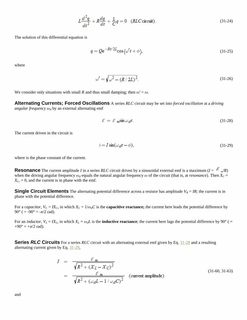
Power In a series RLC circuit, the average power Pavg of the generator is equal to the production rate of thermal energy in the

resistor:

(71, 76)

Here rms stands for root-mean-square; the rms quantities are related to the maximum quantities by ,

and . The term cos is called the power factor of the circuit.

Transformers A transformer (assumed to be ideal) is an iron core on which are wound a primary coil of Np turns and a

secondary coil of Ns turns. If the primary coil is connected across an alternating-current generator, the primary and secondary

voltages are related by

(31-79)

The currents through the coils are related by

(31-80)

and the equivalent resistance of the secondary circuit, as seen by the generator, is

(31-82)

where R is the resistive load in the secondary circuit. The ratio Np/Ns is called the transformer's turns ratio.

Copyright © 2011 John Wiley & Sons, Inc. All rights reserved.

QUESTIONS

1 Figure 31-19 shows three oscillating LC circuits with identical inductors and capacitors. Rank the circuits

according to the time taken to fully discharge the capacitors during the oscillations, greatest first.

Top of Form

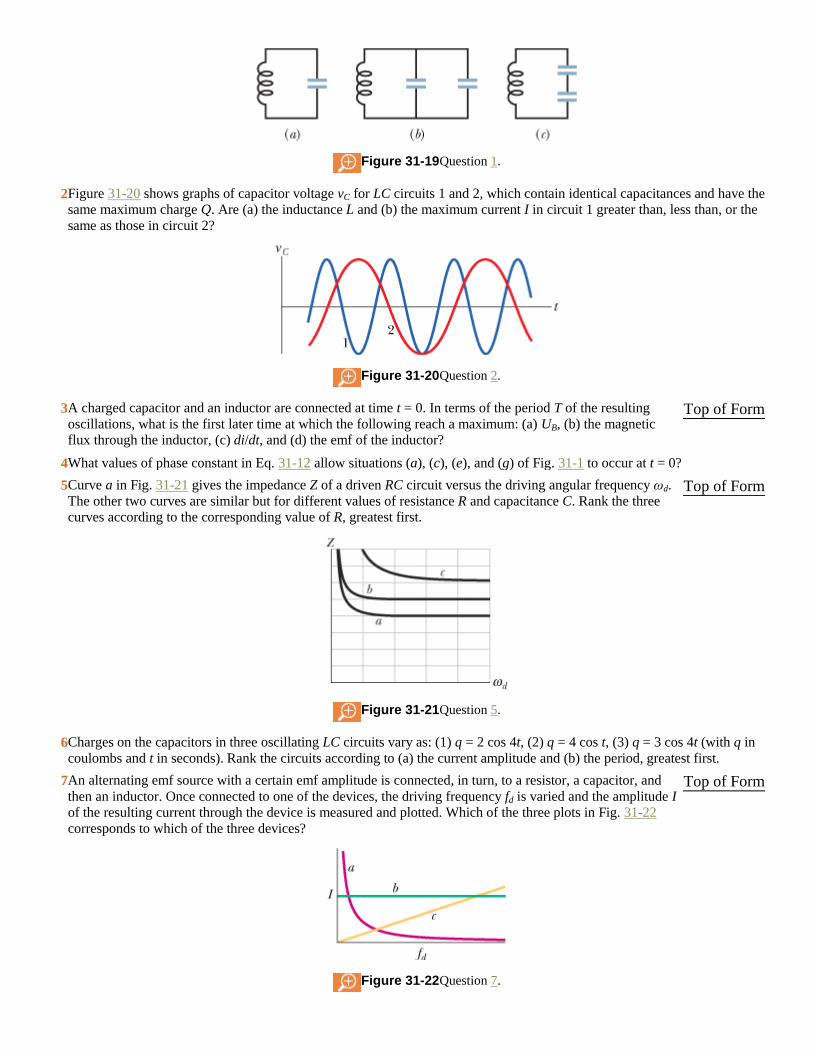
Figure 31-19 Question 1.

2 Figure 31-20 shows graphs of capacitor voltage vC for LC circuits 1 and 2, which contain identical capacitances and have the

same maximum charge Q. Are (a) the inductance L and (b) the maximum current I in circuit 1 greater than, less than, or the

same as those in circuit 2?

Figure 31-20 Question 2.

3 A charged capacitor and an inductor are connected at time t = 0. In terms of the period T of the resulting

oscillations, what is the first later time at which the following reach a maximum: (a) UB, (b) the magnetic

flux through the inductor, (c) di/dt, and (d) the emf of the inductor?

Top of Form

4 What values of phase constant in Eq. 31-12 allow situations (a), (c), (e), and (g) of Fig. 31-1 to occur at t = 0?

5 Curve a in Fig. 31-21 gives the impedance Z of a driven RC circuit versus the driving angular frequency ωd.

The other two curves are similar but for different values of resistance R and capacitance C. Rank the three

curves according to the corresponding value of R, greatest first.

Figure 31-21 Question 5.

Top of Form

6 Charges on the capacitors in three oscillating LC circuits vary as: (1) q = 2 cos 4t, (2) q = 4 cos t, (3) q = 3 cos 4t (with q in

coulombs and t in seconds). Rank the circuits according to (a) the current amplitude and (b) the period, greatest first.

7 An alternating emf source with a certain emf amplitude is connected, in turn, to a resistor, a capacitor, and

then an inductor. Once connected to one of the devices, the driving frequency fd is varied and the amplitude I of the resulting current through the device is measured and plotted. Which of the three plots in Fig. 31-22

corresponds to which of the three devices?

Figure 31-22 Question 7.

Top of Form

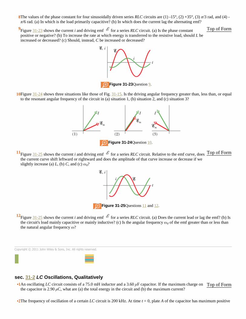
8 The values of the phase constant for four sinusoidally driven series RLC circuits are (1) -15°, (2) +35°, (3) π/3 rad, and (4) -

π/6 rad. (a) In which is the load primarily capacitive? (b) In which does the current lag the alternating emf?

9 Figure 31-23 shows the current i and driving emf for a series RLC circuit. (a) Is the phase constant

positive or negative? (b) To increase the rate at which energy is transferred to the resistive load, should L be

increased or decreased? (c) Should, instead, C be increased or decreased?

Figure 31-23 Question 9.

Top of Form

10 Figure 31-24 shows three situations like those of Fig. 31-15. Is the driving angular frequency greater than, less than, or equal

to the resonant angular frequency of the circuit in (a) situation 1, (b) situation 2, and (c) situation 3?

Figure 31-24 Question 10.

11 Figure 31-25 shows the current i and driving emf for a series RLC circuit. Relative to the emf curve, does

the current curve shift leftward or rightward and does the amplitude of that curve increase or decrease if we

slightly increase (a) L, (b) C, and (c) ωd?

Figure 31-25 Questions 11 and 12.

Top of Form

12 Figure 31-25 shows the current i and driving emf for a series RLC circuit. (a) Does the current lead or lag the emf? (b) Is

the circuit's load mainly capacitive or mainly inductive? (c) Is the angular frequency ωd of the emf greater than or less than

the natural angular frequency ω?

Copyright © 2011 John Wiley & Sons, Inc. All rights reserved.

PROBLEMS

sec. 31-2 LC Oscillations, Qualitatively

•1 An oscillating LC circuit consists of a 75.0 mH inductor and a 3.60 μF capacitor. If the maximum charge on

the capacitor is 2.90 μC, what are (a) the total energy in the circuit and (b) the maximum current? Top of Form

•2 The frequency of oscillation of a certain LC circuit is 200 kHz. At time t = 0, plate A of the capacitor has maximum positive

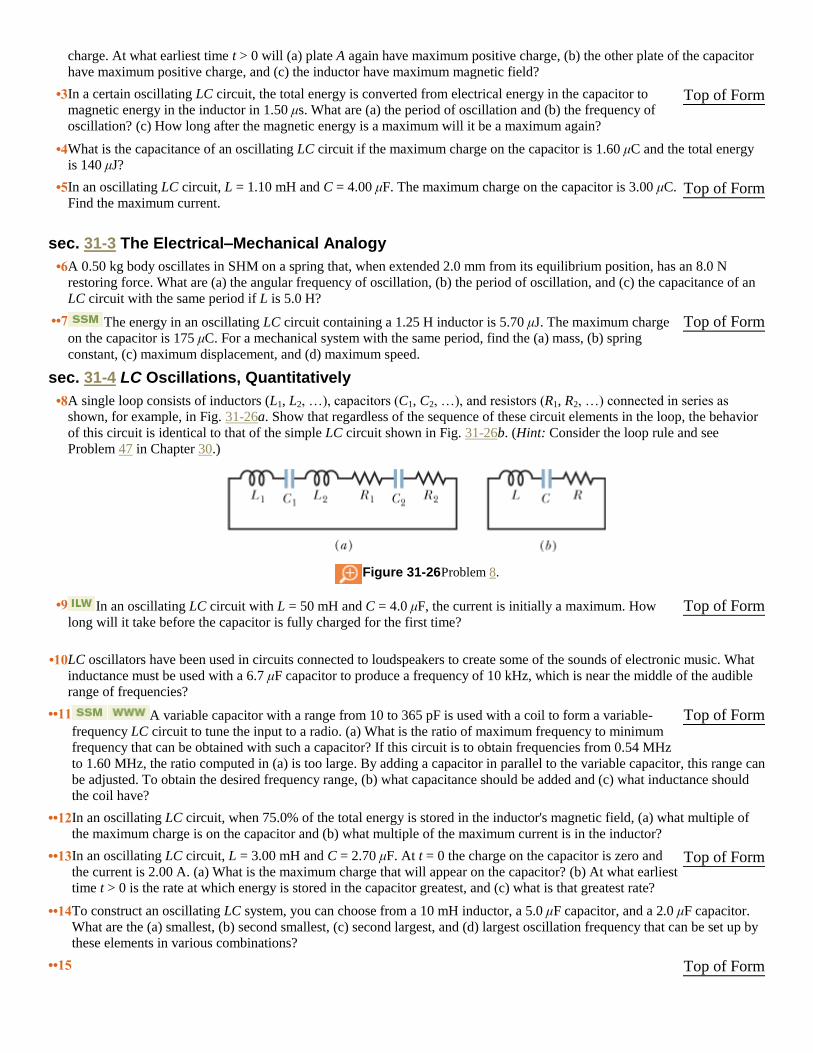
charge. At what earliest time t > 0 will (a) plate A again have maximum positive charge, (b) the other plate of the capacitor

have maximum positive charge, and (c) the inductor have maximum magnetic field?

•3 In a certain oscillating LC circuit, the total energy is converted from electrical energy in the capacitor to

magnetic energy in the inductor in 1.50 μs. What are (a) the period of oscillation and (b) the frequency of

oscillation? (c) How long after the magnetic energy is a maximum will it be a maximum again?

Top of Form

•4 What is the capacitance of an oscillating LC circuit if the maximum charge on the capacitor is 1.60 μC and the total energy

is 140 μJ?

•5 In an oscillating LC circuit, L = 1.10 mH and C = 4.00 μF. The maximum charge on the capacitor is 3.00 μC.

Find the maximum current. Top of Form

sec. 31-3 The Electrical–Mechanical Analogy

•6 A 0.50 kg body oscillates in SHM on a spring that, when extended 2.0 mm from its equilibrium position, has an 8.0 N

restoring force. What are (a) the angular frequency of oscillation, (b) the period of oscillation, and (c) the capacitance of an

LC circuit with the same period if L is 5.0 H?

••7 The energy in an oscillating LC circuit containing a 1.25 H inductor is 5.70 μJ. The maximum charge

on the capacitor is 175 μC. For a mechanical system with the same period, find the (a) mass, (b) spring

constant, (c) maximum displacement, and (d) maximum speed.

Top of Form

sec. 31-4 LC Oscillations, Quantitatively

•8 A single loop consists of inductors (L1, L2, …), capacitors (C1, C2, …), and resistors (R1, R2, …) connected in series as

shown, for example, in Fig. 31-26a. Show that regardless of the sequence of these circuit elements in the loop, the behavior

of this circuit is identical to that of the simple LC circuit shown in Fig. 31-26b. (Hint: Consider the loop rule and see

Problem 47 in Chapter 30.)

Figure 31-26 Problem 8.

•9 In an oscillating LC circuit with L = 50 mH and C = 4.0 μF, the current is initially a maximum. How

long will it take before the capacitor is fully charged for the first time? Top of Form

•10 LC oscillators have been used in circuits connected to loudspeakers to create some of the sounds of electronic music. What

inductance must be used with a 6.7 μF capacitor to produce a frequency of 10 kHz, which is near the middle of the audible

range of frequencies?

••11 A variable capacitor with a range from 10 to 365 pF is used with a coil to form a variable-

frequency LC circuit to tune the input to a radio. (a) What is the ratio of maximum frequency to minimum

frequency that can be obtained with such a capacitor? If this circuit is to obtain frequencies from 0.54 MHz

to 1.60 MHz, the ratio computed in (a) is too large. By adding a capacitor in parallel to the variable capacitor, this range can

be adjusted. To obtain the desired frequency range, (b) what capacitance should be added and (c) what inductance should

the coil have?

Top of Form

••12 In an oscillating LC circuit, when 75.0% of the total energy is stored in the inductor's magnetic field, (a) what multiple of

the maximum charge is on the capacitor and (b) what multiple of the maximum current is in the inductor?

••13 In an oscillating LC circuit, L = 3.00 mH and C = 2.70 μF. At t = 0 the charge on the capacitor is zero and

the current is 2.00 A. (a) What is the maximum charge that will appear on the capacitor? (b) At what earliest

time t > 0 is the rate at which energy is stored in the capacitor greatest, and (c) what is that greatest rate?

Top of Form

••14 To construct an oscillating LC system, you can choose from a 10 mH inductor, a 5.0 μF capacitor, and a 2.0 μF capacitor.

What are the (a) smallest, (b) second smallest, (c) second largest, and (d) largest oscillation frequency that can be set up by

these elements in various combinations?

••15 Top of Form

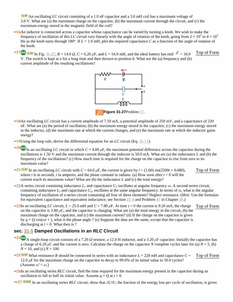
An oscillating LC circuit consisting of a 1.0 nF capacitor and a 3.0 mH coil has a maximum voltage of

3.0 V. What are (a) the maximum charge on the capacitor, (b) the maximum current through the circuit, and (c) the

maximum energy stored in the magnetic field of the coil?

••16 An inductor is connected across a capacitor whose capacitance can be varied by turning a knob. We wish to make the

frequency of oscillation of this LC circuit vary linearly with the angle of rotation of the knob, going from 2 × 105 to 4 × 10

5

Hz as the knob turns through 180°. If L = 1.0 mH, plot the required capacitance C as a function of the angle of rotation of

the knob.

••17 In Fig. 31-27, R = 14.0 Ω, C = 6.20 μF, and L = 54.0 mH, and the ideal battery has emf = 34.0

V. The switch is kept at a for a long time and then thrown to position b. What are the (a) frequency and (b)

current amplitude of the resulting oscillations?

Figure 31-27 Problem 17.

Top of Form

••18 An oscillating LC circuit has a current amplitude of 7.50 mA, a potential amplitude of 250 mV, and a capacitance of 220

nF. What are (a) the period of oscillation, (b) the maximum energy stored in the capacitor, (c) the maximum energy stored

in the inductor, (d) the maximum rate at which the current changes, and (e) the maximum rate at which the inductor gains

energy?

••19 Using the loop rule, derive the differential equation for an LC circuit (Eq. 31-11).

••20 In an oscillating LC circuit in which C = 4.00 μF, the maximum potential difference across the capacitor during the

oscillations is 1.50 V and the maximum current through the inductor is 50.0 mA. What are (a) the inductance L and (b) the

frequency of the oscillations? (c) How much time is required for the charge on the capacitor to rise from zero to its

maximum value?

••21 In an oscillating LC circuit with C = 64.0 μF, the current is given by i = (1.60) sin(2500t + 0.680),

where t is in seconds, i in amperes, and the phase constant in radians. (a) How soon after t = 0 will the

current reach its maximum value? What are (b) the inductance L and (c) the total energy?

Top of Form

••22 A series circuit containing inductance L1 and capacitance C1 oscillates at angular frequency ω. A second series circuit,

containing inductance L2 and capacitance C2, oscillates at the same angular frequency. In terms of ω, what is the angular

frequency of oscillation of a series circuit containing all four of these elements? Neglect resistance. (Hint: Use the formulas

for equivalent capacitance and equivalent inductance; see Section 25-4 and Problem 47 in Chapter 30.)

••23 In an oscillating LC circuit, L = 25.0 mH and C = 7.80 μF. At time t = 0 the current is 9.20 mA, the charge

on the capacitor is 3.80 μC, and the capacitor is charging. What are (a) the total energy in the circuit, (b) the

maximum charge on the capacitor, and (c) the maximum current? (d) If the charge on the capacitor is given

by q = Q cos(ωt + ), what is the phase angle ? (e) Suppose the data are the same, except that the capacitor is

discharging at t = 0. What then is ?

Top of Form

sec. 31-5 Damped Oscillations in an RLC Circuit

••24 A single-loop circuit consists of a 7.20 Ω resistor, a 12.0 H inductor, and a 3.20 μF capacitor. Initially the capacitor has

a charge of 6.20 μC and the current is zero. Calculate the charge on the capacitor N complete cycles later for (a) N = 5, (b)

N = 10, and (c) N = 100.

••25 What resistance R should be connected in series with an inductance L = 220 mH and capacitance C =

12.0 μF for the maximum charge on the capacitor to decay to 99.0% of its initial value in 50.0 cycles?

(Assume ω′ ≈ ω.)

Top of Form

••26 In an oscillating series RLC circuit, find the time required for the maximum energy present in the capacitor during an

oscillation to fall to half its initial value. Assume q = Q at t = 0.

•••27 In an oscillating series RLC circuit, show that ΔU/U, the fraction of the energy lost per cycle of oscillation, is given

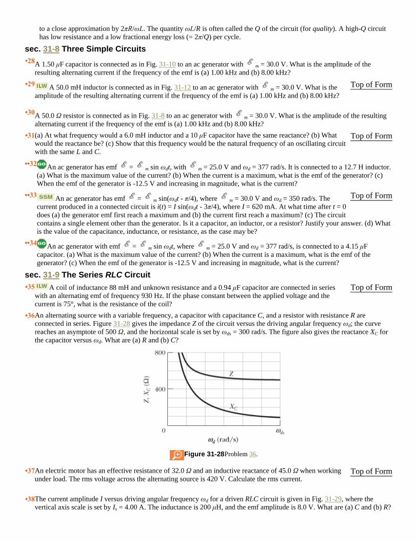
to a close approximation by 2πR/ωL. The quantity ωL/R is often called the Q of the circuit (for quality). A high-Q circuit

has low resistance and a low fractional energy loss (= 2π/Q) per cycle.

sec. 31-8 Three Simple Circuits

•28 A 1.50 μF capacitor is connected as in Fig. 31-10 to an ac generator with m = 30.0 V. What is the amplitude of the

resulting alternating current if the frequency of the emf is (a) 1.00 kHz and (b) 8.00 kHz?

•29 A 50.0 mH inductor is connected as in Fig. 31-12 to an ac generator with m = 30.0 V. What is the

amplitude of the resulting alternating current if the frequency of the emf is (a) 1.00 kHz and (b) 8.00 kHz?

Top of Form

•30 A 50.0 Ω resistor is connected as in Fig. 31-8 to an ac generator with m = 30.0 V. What is the amplitude of the resulting

alternating current if the frequency of the emf is (a) 1.00 kHz and (b) 8.00 kHz?

•31 (a) At what frequency would a 6.0 mH inductor and a 10 μF capacitor have the same reactance? (b) What

would the reactance be? (c) Show that this frequency would be the natural frequency of an oscillating circuit

with the same L and C.

Top of Form

••32 An ac generator has emf = m sin ωdt, with m = 25.0 V and ωd = 377 rad/s. It is connected to a 12.7 H inductor.

(a) What is the maximum value of the current? (b) When the current is a maximum, what is the emf of the generator? (c)

When the emf of the generator is -12.5 V and increasing in magnitude, what is the current?

••33 An ac generator has emf = m sin(ωdt - π/4), where m = 30.0 V and ωd = 350 rad/s. The

current produced in a connected circuit is i(t) = I sin(ωdt - 3π/4), where I = 620 mA. At what time after t = 0

does (a) the generator emf first reach a maximum and (b) the current first reach a maximum? (c) The circuit

contains a single element other than the generator. Is it a capacitor, an inductor, or a resistor? Justify your answer. (d) What

is the value of the capacitance, inductance, or resistance, as the case may be?

Top of Form

••34 An ac generator with emf = m sin ωdt, where m = 25.0 V and ωd = 377 rad/s, is connected to a 4.15 μF

capacitor. (a) What is the maximum value of the current? (b) When the current is a maximum, what is the emf of the

generator? (c) When the emf of the generator is -12.5 V and increasing in magnitude, what is the current?

sec. 31-9 The Series RLC Circuit

•35 A coil of inductance 88 mH and unknown resistance and a 0.94 μF capacitor are connected in series

with an alternating emf of frequency 930 Hz. If the phase constant between the applied voltage and the

current is 75°, what is the resistance of the coil?

Top of Form

•36 An alternating source with a variable frequency, a capacitor with capacitance C, and a resistor with resistance R are

connected in series. Figure 31-28 gives the impedance Z of the circuit versus the driving angular frequency ωd; the curve

reaches an asymptote of 500 Ω, and the horizontal scale is set by ωds = 300 rad/s. The figure also gives the reactance XC for

the capacitor versus ωd. What are (a) R and (b) C?

Figure 31-28 Problem 36.

•37 An electric motor has an effective resistance of 32.0 Ω and an inductive reactance of 45.0 Ω when working

under load. The rms voltage across the alternating source is 420 V. Calculate the rms current. Top of Form

•38 The current amplitude I versus driving angular frequency ωd for a driven RLC circuit is given in Fig. 31-29, where the

vertical axis scale is set by Is = 4.00 A. The inductance is 200 μH, and the emf amplitude is 8.0 V. What are (a) C and (b) R?

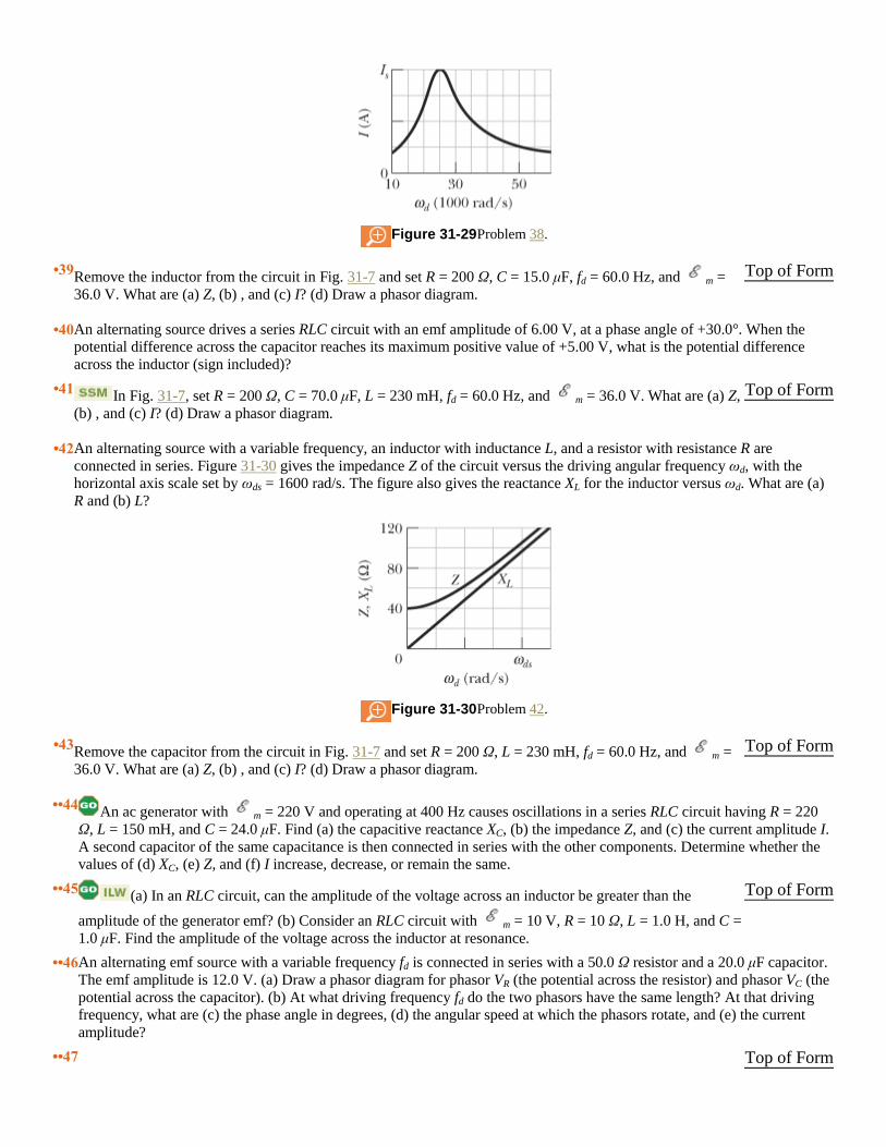
Figure 31-29 Problem 38.

•39 Remove the inductor from the circuit in Fig. 31-7 and set R = 200 Ω, C = 15.0 μF, fd = 60.0 Hz, and m =

36.0 V. What are (a) Z, (b) , and (c) I? (d) Draw a phasor diagram.

Top of Form

•40 An alternating source drives a series RLC circuit with an emf amplitude of 6.00 V, at a phase angle of +30.0°. When the

potential difference across the capacitor reaches its maximum positive value of +5.00 V, what is the potential difference

across the inductor (sign included)?

•41 In Fig. 31-7, set R = 200 Ω, C = 70.0 μF, L = 230 mH, fd = 60.0 Hz, and m = 36.0 V. What are (a) Z,

(b) , and (c) I? (d) Draw a phasor diagram.

Top of Form

•42 An alternating source with a variable frequency, an inductor with inductance L, and a resistor with resistance R are

connected in series. Figure 31-30 gives the impedance Z of the circuit versus the driving angular frequency ωd, with the

horizontal axis scale set by ωds = 1600 rad/s. The figure also gives the reactance XL for the inductor versus ωd. What are (a)

R and (b) L?

Figure 31-30 Problem 42.

•43 Remove the capacitor from the circuit in Fig. 31-7 and set R = 200 Ω, L = 230 mH, fd = 60.0 Hz, and m =

36.0 V. What are (a) Z, (b) , and (c) I? (d) Draw a phasor diagram.

Top of Form

••44 An ac generator with m = 220 V and operating at 400 Hz causes oscillations in a series RLC circuit having R = 220

Ω, L = 150 mH, and C = 24.0 μF. Find (a) the capacitive reactance XC, (b) the impedance Z, and (c) the current amplitude I.

A second capacitor of the same capacitance is then connected in series with the other components. Determine whether the

values of (d) XC, (e) Z, and (f) I increase, decrease, or remain the same.

••45 (a) In an RLC circuit, can the amplitude of the voltage across an inductor be greater than the

amplitude of the generator emf? (b) Consider an RLC circuit with m = 10 V, R = 10 Ω, L = 1.0 H, and C =

1.0 μF. Find the amplitude of the voltage across the inductor at resonance.

Top of Form

••46 An alternating emf source with a variable frequency fd is connected in series with a 50.0 Ω resistor and a 20.0 μF capacitor.

The emf amplitude is 12.0 V. (a) Draw a phasor diagram for phasor VR (the potential across the resistor) and phasor VC (the

potential across the capacitor). (b) At what driving frequency fd do the two phasors have the same length? At that driving

frequency, what are (c) the phase angle in degrees, (d) the angular speed at which the phasors rotate, and (e) the current

amplitude?

••47 Top of Form

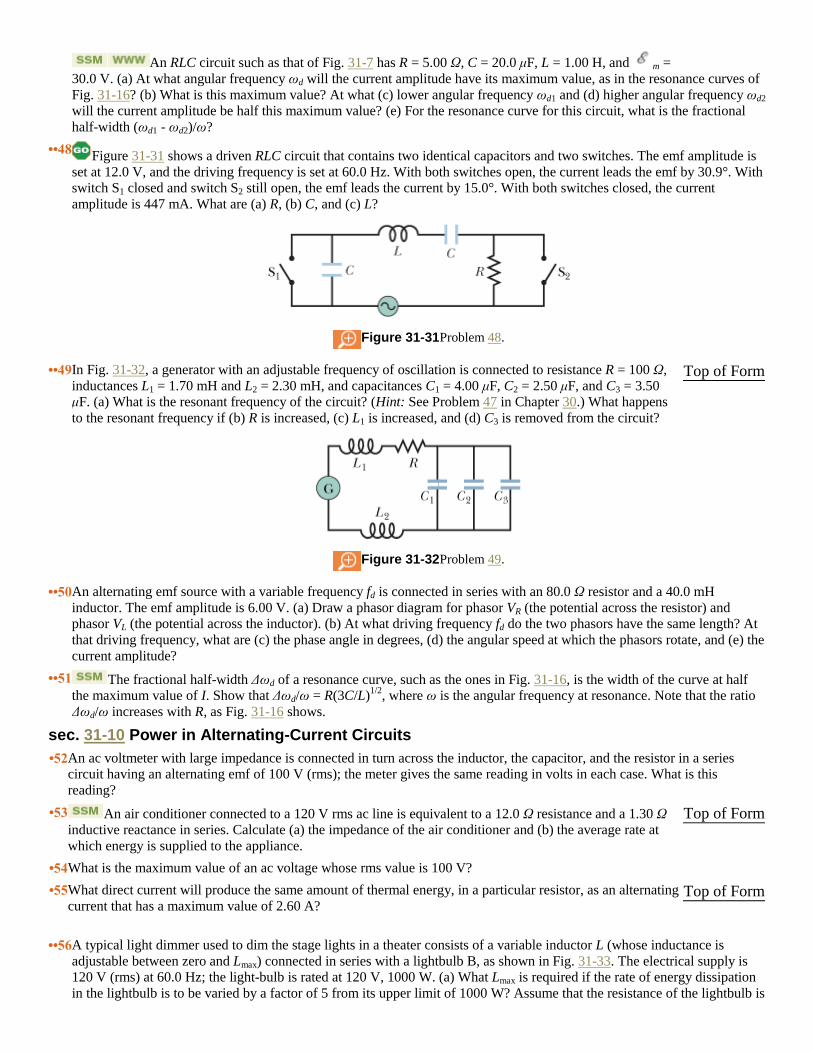
An RLC circuit such as that of Fig. 31-7 has R = 5.00 Ω, C = 20.0 μF, L = 1.00 H, and m =

30.0 V. (a) At what angular frequency ωd will the current amplitude have its maximum value, as in the resonance curves of

Fig. 31-16? (b) What is this maximum value? At what (c) lower angular frequency ωd1 and (d) higher angular frequency ωd2

will the current amplitude be half this maximum value? (e) For the resonance curve for this circuit, what is the fractional

half-width (ωd1 - ωd2)/ω?

••48 Figure 31-31 shows a driven RLC circuit that contains two identical capacitors and two switches. The emf amplitude is

set at 12.0 V, and the driving frequency is set at 60.0 Hz. With both switches open, the current leads the emf by 30.9°. With

switch S1 closed and switch S2 still open, the emf leads the current by 15.0°. With both switches closed, the current

amplitude is 447 mA. What are (a) R, (b) C, and (c) L?

Figure 31-31 Problem 48.

••49 In Fig. 31-32, a generator with an adjustable frequency of oscillation is connected to resistance R = 100 Ω,

inductances L1 = 1.70 mH and L2 = 2.30 mH, and capacitances C1 = 4.00 μF, C2 = 2.50 μF, and C3 = 3.50

μF. (a) What is the resonant frequency of the circuit? (Hint: See Problem 47 in Chapter 30.) What happens

to the resonant frequency if (b) R is increased, (c) L1 is increased, and (d) C3 is removed from the circuit?

Figure 31-32 Problem 49.

Top of Form

••50 An alternating emf source with a variable frequency fd is connected in series with an 80.0 Ω resistor and a 40.0 mH

inductor. The emf amplitude is 6.00 V. (a) Draw a phasor diagram for phasor VR (the potential across the resistor) and

phasor VL (the potential across the inductor). (b) At what driving frequency fd do the two phasors have the same length? At

that driving frequency, what are (c) the phase angle in degrees, (d) the angular speed at which the phasors rotate, and (e) the

current amplitude?

••51 The fractional half-width Δωd of a resonance curve, such as the ones in Fig. 31-16, is the width of the curve at half

the maximum value of I. Show that Δωd/ω = R(3C/L)1/2

, where ω is the angular frequency at resonance. Note that the ratio

Δωd/ω increases with R, as Fig. 31-16 shows.

sec. 31-10 Power in Alternating-Current Circuits

•52 An ac voltmeter with large impedance is connected in turn across the inductor, the capacitor, and the resistor in a series

circuit having an alternating emf of 100 V (rms); the meter gives the same reading in volts in each case. What is this

reading?

•53 An air conditioner connected to a 120 V rms ac line is equivalent to a 12.0 Ω resistance and a 1.30 Ω

inductive reactance in series. Calculate (a) the impedance of the air conditioner and (b) the average rate at

which energy is supplied to the appliance.

Top of Form

•54 What is the maximum value of an ac voltage whose rms value is 100 V?

•55 What direct current will produce the same amount of thermal energy, in a particular resistor, as an alternating

current that has a maximum value of 2.60 A? Top of Form

••56 A typical light dimmer used to dim the stage lights in a theater consists of a variable inductor L (whose inductance is

adjustable between zero and Lmax) connected in series with a lightbulb B, as shown in Fig. 31-33. The electrical supply is

120 V (rms) at 60.0 Hz; the light-bulb is rated at 120 V, 1000 W. (a) What Lmax is required if the rate of energy dissipation

in the lightbulb is to be varied by a factor of 5 from its upper limit of 1000 W? Assume that the resistance of the lightbulb is

independent of its temperature. (b) Could one use a variable resistor (adjustable between zero and Rmax) instead of an

inductor? (c) If so, what Rmax is required? (d) Why isn't this done?

Figure 31-33 Problem 56.

••57 In an RLC circuit such as that of Fig. 31-7 assume that R = 5.00 Ω, L = 60.0 mH, fd = 60.0 Hz, and m =

30.0 V. For what values of the capacitance would the average rate at which energy is dissipated in the

resistance be (a) a maximum and (b) a minimum? What are (c) the maximum dissipation rate and the

corresponding (d) phase angle and (e) power factor? What are (f) the minimum dissipation rate and the corresponding (g)

phase angle and (h) power factor?

Top of Form

••58 For Fig. 31-34, show that the average rate at which energy is dissipated in resistance R is a maximum when R is equal to the

internal resistance r of the ac generator. (In the text discussion we tacitly assumed that r = 0.)

Figure 31-34 Problems 58 and 66.

••59 In Fig. 31-7, R = 15.0 Ω, C = 4.70 μF, and L = 25.0 mH. The generator provides an emf with rms voltage

75.0 V and frequency 550 Hz. (a) What is the rms current? What is the rms voltage across (b) R, (c) C, (d) L,

(e) C and L together, and (f) R, C, and L together? At what average rate is energy dissipated by (g) R, (h) C,

and (i) L?

Top of Form

••60 In a series oscillating RLC circuit, R = 16.0 Ω, C = 31.2 μF, L = 9.20 mH, and m = m sin ωdt with m = 45.0 V

and ωd = 3000 rad/s. For time t = 0.442 ms find (a) the rate Pg at which energy is being supplied by the generator, (b) the

rate PC at which the energy in the capacitor is changing, (c) the rate PL at which the energy in the inductor is changing, and

(d) the rate PR at which energy is being dissipated in the resistor. (e) Is the sum of PC, PL, and PR greater than, less than, or

equal to Pg?

••61 Figure 31-35 shows an ac generator connected to a “black box” through a pair of terminals.

The box contains an RLC circuit, possibly even a multiloop circuit, whose elements and connections we do

not know. Measurements outside the box reveal that

and

(a) What is the power factor? (b) Does the current lead or lag the emf? (c) Is the circuit in the box largely inductive or

largely capacitive? (d) Is the circuit in the box in resonance? (e) Must there be a capacitor in the box? (f) An inductor? (g) A

resistor? (h) At what average rate is energy delivered to the box by the generator? (i) Why don't you need to know ωd to

answer all these questions?

Figure 31-35 Problem 61.

Top of Form

sec. 31-11 Transformers

•62 A generator supplies 100 V to a transformer's primary coil, which has 50 turns. If the secondary coil has 500 turns, what is

the secondary voltage?

•63 A transformer has 500 primary turns and 10 secondary turns. (a) If Vp is 120 V (rms), what is Vs

with an open circuit? If the secondary now has a resistive load of 15 Ω, what is the current in the (b) primary

and (c) secondary?

Top of Form

•64 Figure 31-36 shows an “autotransformer.” It consists of a single coil (with an iron core). Three taps Ti are provided.

Between taps T1 and T2 there are 200 turns, and between taps T2 and T3 there are 800 turns. Any two taps can be chosen as

the primary terminals, and any two taps can be chosen as the secondary terminals. For choices producing a step-up

transformer, what are the (a) smallest, (b) second smallest, and (c) largest values of the ratio Vs/Vp? For a step-down

transformer, what are the (d) smallest, (e) second smallest, and (f) largest values of Vs/Vp?

Figure 31-36 Problem 64.

••65 An ac generator provides emf to a resistive load in a remote factory over a two-cable transmission line. At

the factory a step-down transformer reduces the voltage from its (rms) transmission value Vt to a much lower

value that is safe and convenient for use in the factory. The transmission line resistance is 0.30 Ω/cable, and

the power of the generator is 250 kW. If Vt = 80 kV, what are (a) the voltage decrease ΔV along the

transmission line and (b) the rate Pd at which energy is dissipated in the line as thermal energy? If Vt = 8.0 kV, what are (c)

ΔV and (d) Pd? If Vt = 0.80 kV, what are (e) ΔV and (f) Pd?

Top of Form

Additional Problems

66 In Fig. 31-34, let the rectangular box on the left represent the (high-impedance) output of an audio amplifier, with r = 1000

Ω. Let R = 10 Ω represent the (low-impedance) coil of a loudspeaker. For maximum transfer of energy to the load R we

must have R = r, and that is not true in this case. However, a transformer can be used to “transform” resistances, making

them behave electrically as if they were larger or smaller than they actually are. (a) Sketch the primary and secondary coils

of a transformer that can be introduced between the amplifier and the speaker in Fig. 31-34 to match the impedances. (b)

What must be the turns ratio?

67 An ac generator produces emf = m sin(ωdt - π/4), where m = 30.0 V and ωd = 350 rad/s. The current

in the circuit attached to the generator is i(t) = I sin(ωdt + π/4), where I = 620 mA. (a) At what time after t = 0

does the generator emf first reach a maximum? (b) At what time after t = 0 does the current first reach a

maximum? (c) The circuit contains a single element other than the generator. Is it a capacitor, an inductor, or a resistor?

Justify your answer. (d) What is the value of the capacitance, inductance, or resistance, as the case may be?

Top of Form

68 A series RLC circuit is driven by a generator at a frequency of 2000 Hz and an emf amplitude of 170 V. The inductance is

60.0 mH, the capacitance is 0.400 μF, and the resistance is 200 Ω. (a) What is the phase constant in radians? (b) What is the

current amplitude?

69 A generator of frequency 3000 Hz drives a series RLC circuit with an emf amplitude of 120 V. The

resistance is 40.0 Ω, the capacitance is 1.60 μF, and the inductance is 850 μH. What are (a) the phase

constant in radians and (b) the current amplitude? (c) Is the circuit capacitive, inductive, or in resonance?

Top of Form

70 A 45.0 mH inductor has a reactance of 1.30 kΩ. (a) What is its operating frequency? (b) What is the capacitance of a capacitor with the same reactance at that frequency? If the frequency is doubled, what is the new reactance of (c) the

inductor and (d) the capacitor?

71 An RLC circuit is driven by a generator with an emf amplitude of 80.0 V and a current amplitude of 1.25 A.

The current leads the emf by 0.650 rad. What are the (a) impedance and (b) resistance of the circuit? (c) Is

the circuit inductive, capacitive, or in resonance?

Top of Form

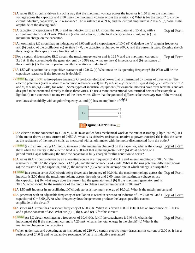
72 A series RLC circuit is driven in such a way that the maximum voltage across the inductor is 1.50 times the maximum

voltage across the capacitor and 2.00 times the maximum voltage across the resistor. (a) What is for the circuit? (b) Is the

circuit inductive, capacitive, or in resonance? The resistance is 49.9 Ω, and the current amplitude is 200 mA. (c) What is the

amplitude of the driving emf?

73 A capacitor of capacitance 158 μF and an inductor form an LC circuit that oscillates at 8.15 kHz, with a

current amplitude of 4.21 mA. What are (a) the inductance, (b) the total energy in the circuit, and (c) the

maximum charge on the capacitor?

Top of Form

74 An oscillating LC circuit has an inductance of 3.00 mH and a capacitance of 10.0 μF. Calculate the (a) angular frequency

and (b) period of the oscillation. (c) At time t = 0, the capacitor is charged to 200 μC and the current is zero. Roughly sketch

the charge on the capacitor as a function of time.

75 For a certain driven series RLC circuit, the maximum generator emf is 125 V and the maximum current is

3.20 A. If the current leads the generator emf by 0.982 rad, what are the (a) impedance and (b) resistance of

the circuit? (c) Is the circuit predominantly capacitive or inductive?

Top of Form

76 A 1.50 μF capacitor has a capacitive reactance of 12.0 Ω. (a) What must be its operating frequency? (b) What will be the

capacitive reactance if the frequency is doubled?

77 In Fig. 31-37, a three-phase generator G produces electrical power that is transmitted by means of three wires. The

electric potentials (each relative to a common reference level) are V1 = A sin ωdt for wire 1, V2 = A sin(ωdt - 120°) for wire 2,

and V3 = A sin(ωdt - 240°) for wire 3. Some types of industrial equipment (for example, motors) have three terminals and are

designed to be connected directly to these three wires. To use a more conventional two-terminal device (for example, a

lightbulb), one connects it to any two of the three wires. Show that the potential difference between any two of the wires (a)

oscillates sinusoidally with angular frequency ωd and (b) has an amplitude of .

Figure 31-37 Problem 77.

78 An electric motor connected to a 120 V, 60.0 Hz ac outlet does mechanical work at the rate of 0.100 hp (1 hp = 746 W). (a)

If the motor draws an rms current of 0.650 A, what is its effective resistance, relative to power transfer? (b) Is this the same

as the resistance of the motor's coils, as measured with an ohmmeter with the motor disconnected from the outlet?

79 (a) In an oscillating LC circuit, in terms of the maximum charge Q on the capacitor, what is the charge

there when the energy in the electric field is 50.0% of that in the magnetic field? (b) What fraction of a

period must elapse following the time the capacitor is fully charged for this condition to occur?

Top of Form

80 A series RLC circuit is driven by an alternating source at a frequency of 400 Hz and an emf amplitude of 90.0 V. The

resistance is 20.0 Ω, the capacitance is 12.1 μF, and the inductance is 24.2 mH. What is the rms potential difference across

(a) the resistor, (b) the capacitor, and (c) the inductor? (d) What is the average rate at which energy is dissipated?

81 In a certain series RLC circuit being driven at a frequency of 60.0 Hz, the maximum voltage across the

inductor is 2.00 times the maximum voltage across the resistor and 2.00 times the maximum voltage across

the capacitor. (a) By what angle does the current lag the generator emf? (b) If the maximum generator emf is

30.0 V, what should be the resistance of the circuit to obtain a maximum current of 300 mA?

Top of Form

82 A 1.50 mH inductor in an oscillating LC circuit stores a maximum energy of 10.0 μJ. What is the maximum current?

83 A generator with an adjustable frequency of oscillation is wired in series to an inductor of L = 2.50 mH and a

capacitor of C = 3.00 μF. At what frequency does the generator produce the largest possible current

amplitude in the circuit?

Top of Form

84 A series RLC circuit has a resonant frequency of 6.00 kHz. When it is driven at 8.00 kHz, it has an impedance of 1.00 kΩ

and a phase constant of 45°. What are (a) R, (b) L, and (c) C for this circuit?

85 An LC circuit oscillates at a frequency of 10.4 kHz. (a) If the capacitance is 340 μF, what is the

inductance? (b) If the maximum current is 7.20 mA, what is the total energy in the circuit? (c) What is the

maximum charge on the capacitor?

Top of Form

86 When under load and operating at an rms voltage of 220 V, a certain electric motor draws an rms current of 3.00 A. It has a

resistance of 24.0 Ω and no capacitive reactance. What is its inductive reactance?

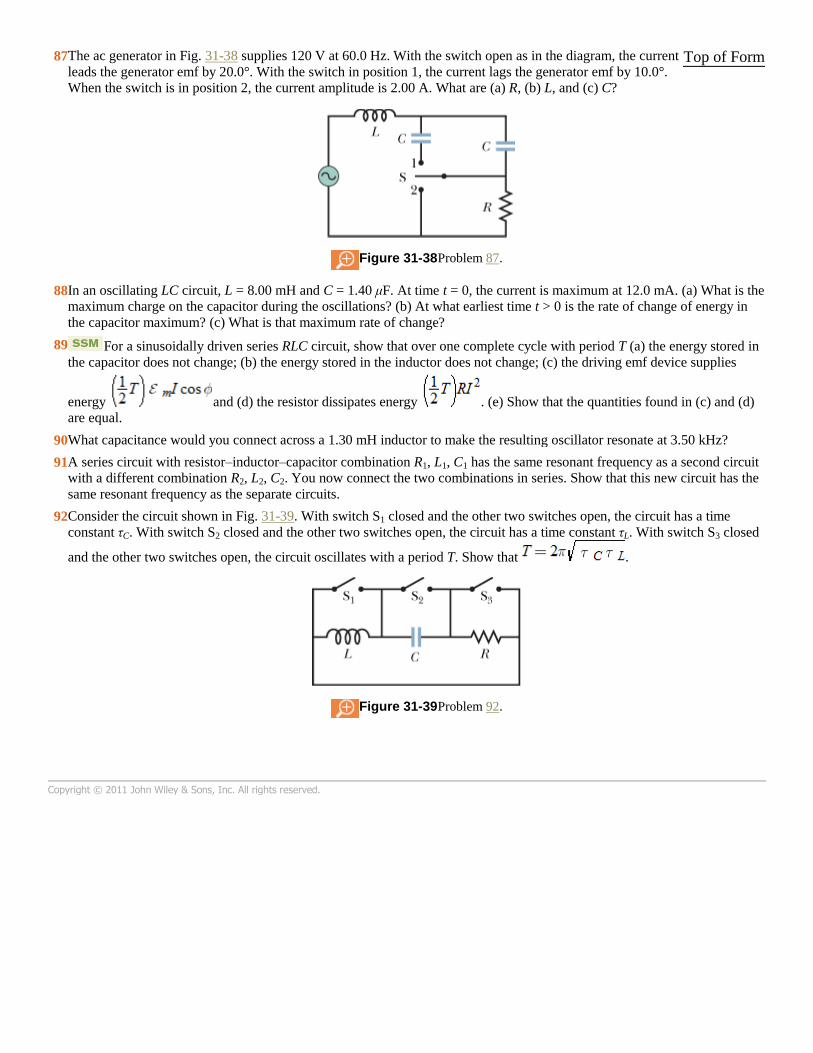
87 The ac generator in Fig. 31-38 supplies 120 V at 60.0 Hz. With the switch open as in the diagram, the current

leads the generator emf by 20.0°. With the switch in position 1, the current lags the generator emf by 10.0°.

When the switch is in position 2, the current amplitude is 2.00 A. What are (a) R, (b) L, and (c) C?

Figure 31-38 Problem 87.

Top of Form

88 In an oscillating LC circuit, L = 8.00 mH and C = 1.40 μF. At time t = 0, the current is maximum at 12.0 mA. (a) What is the

maximum charge on the capacitor during the oscillations? (b) At what earliest time t > 0 is the rate of change of energy in

the capacitor maximum? (c) What is that maximum rate of change?

89 For a sinusoidally driven series RLC circuit, show that over one complete cycle with period T (a) the energy stored in

the capacitor does not change; (b) the energy stored in the inductor does not change; (c) the driving emf device supplies

energy and (d) the resistor dissipates energy . (e) Show that the quantities found in (c) and (d)

are equal.

90 What capacitance would you connect across a 1.30 mH inductor to make the resulting oscillator resonate at 3.50 kHz?

91 A series circuit with resistor–inductor–capacitor combination R1, L1, C1 has the same resonant frequency as a second circuit

with a different combination R2, L2, C2. You now connect the two combinations in series. Show that this new circuit has the

same resonant frequency as the separate circuits.

92 Consider the circuit shown in Fig. 31-39. With switch S1 closed and the other two switches open, the circuit has a time

constant τC. With switch S2 closed and the other two switches open, the circuit has a time constant τL. With switch S3 closed

and the other two switches open, the circuit oscillates with a period T. Show that .

Figure 31-39 Problem 92.

Copyright © 2011 John Wiley & Sons, Inc. All rights reserved.