31 Oct. 2000 15-859B - Introduction to Scientific Computing 1

Initial Value Problems

Paul Heckbert

Computer Science Department

Carnegie Mellon University

31 Oct. 2000 15-859B - Introduction to Scientific Computing 2

Generic First Order ODE

given

y’=f(t,y)

y(t0)=y0

solve for y(t) for t>t0

31 Oct. 2000 15-859B - Introduction to Scientific Computing 3

First ODE:y’=y

• ODE is unstable• (solution is y(t)=cet )

• we show solutions with Euler’s method

31 Oct. 2000 15-859B - Introduction to Scientific Computing 4

y’=y

31 Oct. 2000 15-859B - Introduction to Scientific Computing 5

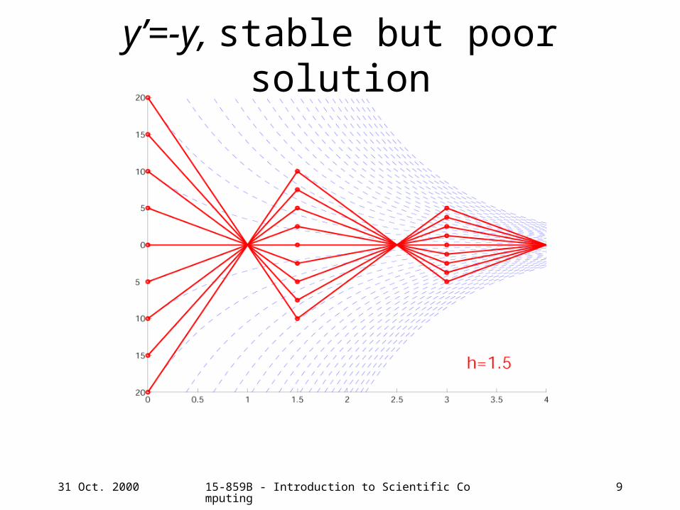
Second ODE:y’=-y

• ODE is stable• (solution is y(t)= ce-t )

• if h too large, numerical solution is unstable

• we show solutions with Euler’s method in red

31 Oct. 2000 15-859B - Introduction to Scientific Computing 6

y’=-y, stable but slow solution

31 Oct. 2000 15-859B - Introduction to Scientific Computing 7

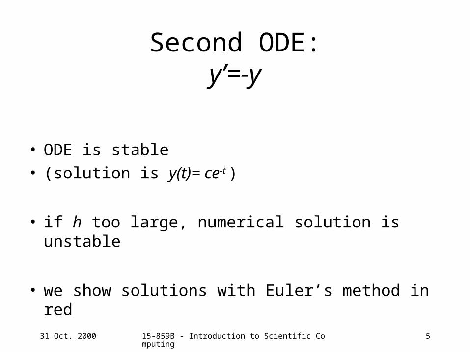
y’=-y, stable, a bit inaccurate soln.

31 Oct. 2000 15-859B - Introduction to Scientific Computing 8

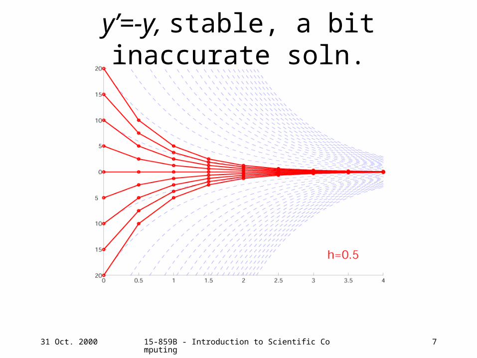
y’=-y, stable, rather inaccurate soln.

31 Oct. 2000 15-859B - Introduction to Scientific Computing 9

y’=-y, stable but poor solution

31 Oct. 2000 15-859B - Introduction to Scientific Computing 10

y’=-y, oscillating solution

31 Oct. 2000 15-859B - Introduction to Scientific Computing 11

y’=-y, unstable solution

31 Oct. 2000 15-859B - Introduction to Scientific Computing 12

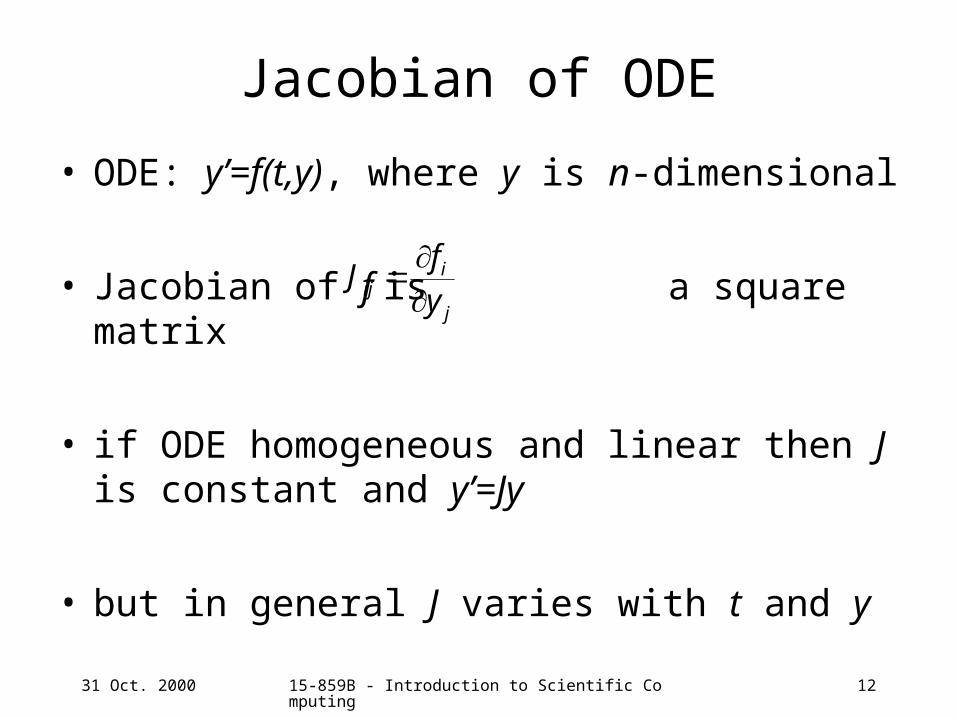
Jacobian of ODE

• ODE: y’=f(t,y), where y is n-dimensional

• Jacobian of f is a square matrix

• if ODE homogeneous and linear then J is constant and y’=Jy

• but in general J varies with t and y

j

iij y

fJ

31 Oct. 2000 15-859B - Introduction to Scientific Computing 13

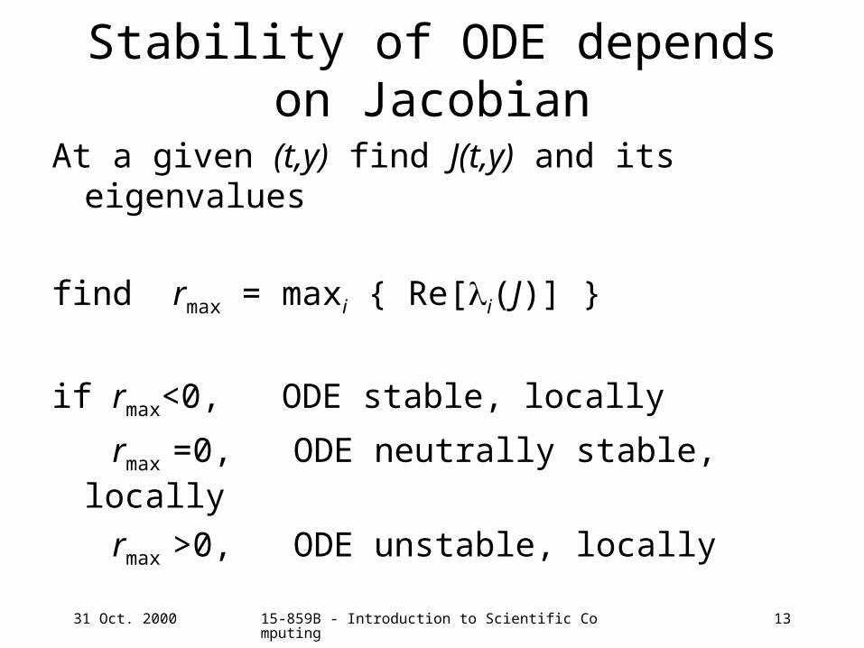
Stability of ODE depends on Jacobian

At a given (t,y) find J(t,y) and its eigenvalues

find rmax = maxi { Re[i(J)] }

if rmax<0, ODE stable, locally

rmax =0, ODE neutrally stable, locally

rmax >0, ODE unstable, locally

31 Oct. 2000 15-859B - Introduction to Scientific Computing 14

Stability of Numerical Solution

• Stability of numerical solution is related to, but not the same as stability of ODE!

• Amplification factor of a numerical solution is the factor by which global error grows or shrinks each iteration.

31 Oct. 2000 15-859B - Introduction to Scientific Computing 15

Stability of Euler’s Method

• Amplification factor of Euler’s method is I+hJ• Note that it depends on h and, in general, on t & y.• Stability of Euler’s method is determined by

eigenvalues of I+hJ

• spectral radius (I+hJ)= maxi | i(I+hJ) |

• if (I+hJ)<1 then Euler’s method stable– if all eigenvalues of hJ lie inside unit circle centered at –1,

E.M. is stable

– scalar case: 0<|hJ|<2 iff stable, so choose h < 2/|J|

• What if one eigenvalue of J is much larger than the others?

31 Oct. 2000 15-859B - Introduction to Scientific Computing 16

Stiff ODE

• An ODE is stiff if its eigenvalues have greatly differing magnitudes.

• With a stiff ODE, one eigenvalue can force use of small h when using Euler’s method

31 Oct. 2000 15-859B - Introduction to Scientific Computing 17

Implicit Methods

• use information from future time tk+1 to take a step from tk

• Euler method: yk+1 = yk+f(tk,yk)hk

• backward Euler method: yk+1 = yk+f(tk+1,yk+1)hk

• example:• y’=Ay f(t,y)=Ay

• yk+1 = yk+Ayk+1hk

• (I-hkA)yk+1=yk -- solve this system each iteration

31 Oct. 2000 15-859B - Introduction to Scientific Computing 18

Stability of Backward Euler’s Method

• Amplification factor of B.E.M. is (I-hJ)-1

• B.E.M. is stable independent of h (unconditionally stable) as long as rmax<0, i.e. as long as ODE is stable

• Implicit methods such as this permit bigger steps to be taken (larger h)

31 Oct. 2000 15-859B - Introduction to Scientific Computing 19

y’=-y, B.E.M. with large step

31 Oct. 2000 15-859B - Introduction to Scientific Computing 20

y’=-y, B.E.M. with very large step

31 Oct. 2000 15-859B - Introduction to Scientific Computing 21

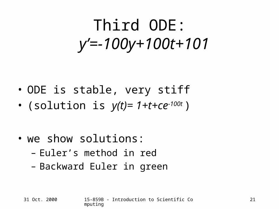
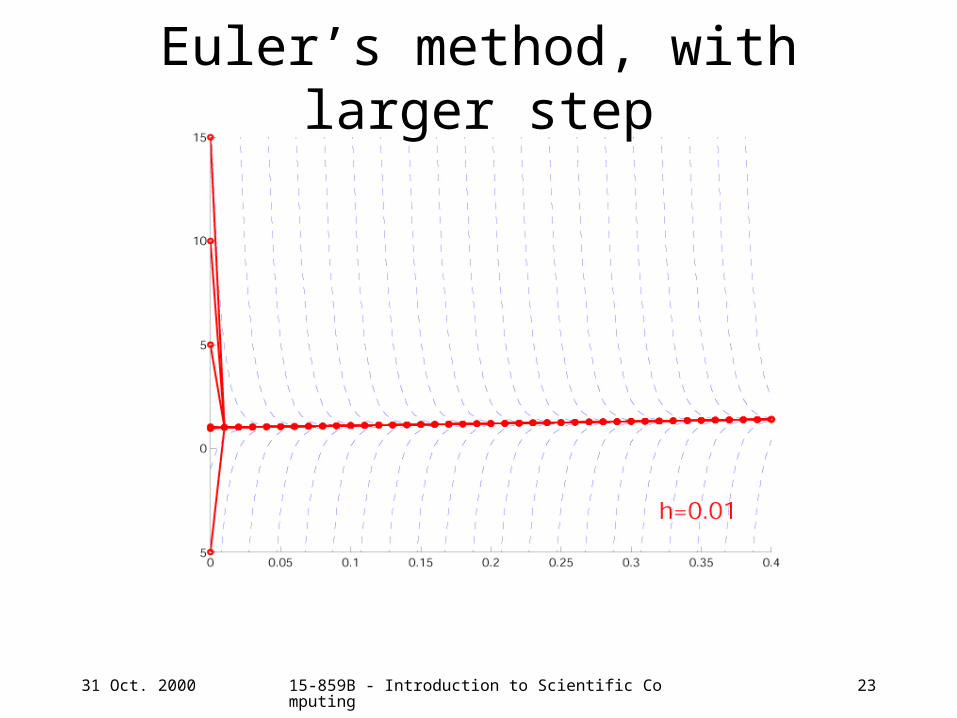
Third ODE: y’=-100y+100t+101

• ODE is stable, very stiff• (solution is y(t)= 1+t+ce-100t )

• we show solutions:– Euler’s method in red

– Backward Euler in green

31 Oct. 2000 15-859B - Introduction to Scientific Computing 22

Euler’s method requires tiny step

31 Oct. 2000 15-859B - Introduction to Scientific Computing 23

Euler’s method, with larger step

31 Oct. 2000 15-859B - Introduction to Scientific Computing 24

Euler’s method with too large a step

three solutions started at y0=.99, 1, 1.01

31 Oct. 2000 15-859B - Introduction to Scientific Computing 25

Large steps OK with Backward Euler’s method

31 Oct. 2000 15-859B - Introduction to Scientific Computing 26

Very large steps OK, too

31 Oct. 2000 15-859B - Introduction to Scientific Computing 27

Popular IVP Solution Methods

• Euler’s method, 1st order• backward Euler’s method, 1st order• trapezoid method (a.k.a. 2nd order Adams-Moulton)• 4th order Runge-Kutta

• If a method is pth order accurate then its global error is O(hp)

31 Oct. 2000 15-859B - Introduction to Scientific Computing 28

Matlab code used to make E.M. plots• function [tv,yv] = euler(funcname,h,t0,tmax,y0)

% use Euler's method to solve y'=func(t,y)% return tvec and yvec sampled at t=(t0:h:tmax) as col. vectors% funcname is a string containing the name of func% apparently func has to be in this file??

% Paul Heckbert 30 Oct 2000

y = y0;tv = [t0];yv = [y0];for t = t0:h:tmax f = eval([funcname '(t,y)']); y = y+f*h; tv = [tv; t+h]; yv = [yv; y];end

function f = func1(t,y) % Heath fig 9.6f = y;return;

function f = func2(t,y) % Heath fig 9.7f = -y;return;

function f = func3(t,y) % Heath example 9.11f = -100*y+100*t+101;return;

31 Oct. 2000 15-859B - Introduction to Scientific Computing 29

Matlab code used to make E.M. plots• function e3(h,file)

figure(4);clf;hold on;tmax = .4;axis([0 tmax -5 15]);% axis([0 .05 .95 2]);

% first draw "exact" solution in bluey0v = 2.^(0:4:80);for y0 = [y0v -y0v] [tv,yv] = euler('func3', .005, 0, tmax, y0); plot(tv,yv,'b--');end

% then draw approximate solution in redfor y0 = [(.95:.05:1.05) -5 5 10 15] [tv,yv] = euler('func3', h, 0, tmax, y0); plot(tv,yv,'ro-', 'LineWidth',2, 'MarkerSize',4);endtext(.32,-3, sprintf('h=%g', h), 'FontSize',20, 'Color','r');

eval(['print -depsc2 ' file]);

• run, e.g. e3(.1, ‘a.eps’)