3.2 .4 The leapf ro g sc he m e is st able fo r the osci

Mixed and Implicit Schemes §3.2.4

The leapfrog scheme is stable for the oscillation equation andunstable for the friction equation.



The Euler forward scheme is stable for the friction equationbut unstable for the oscillation equation.




Suppose we require an approximation to the equation

dU

dt= iωU − κU ,

This is a prototype of the N.S equations, with terms of both types.




Suppose we require an approximation to the equation

dU

dt= iωU − κU ,


One approach is to use the leapfrog scheme for the oscil-lation term and the forward scheme for the friction term:

Un+1 = Un−1 + 2∆t(iωUn − κUn−1) .




Suppose we require an approximation to the equationdU

dt= iωU − κU ,


One approach is to use the leapfrog scheme for the oscil-lation term and the forward scheme for the friction term:

Un+1 = Un−1 + 2∆t(iωUn − κUn−1) .

We can show that this is stable provided

(2κ∆t + ω2∆t2) ≤ 1 .

Modern numerical models of the atmosphere typically com-bine several distinct schemes in this way.

2


The Navier-Stokes equations are

∂V

∂t+ V ·∇V + 2Ω×V +

1

ρ∇p = ν∇2V + g .

They have advection terms corresponding to the oscillationequation and diffusion terms like the friction equation.

2



∂V

∂t+ V ·∇V + 2Ω×V +

1

ρ∇p = ν∇2V + g .


We will shortly consider the semi-implicit scheme, wheresome terms are integrated implicitly and others explicitly.

& & &

2



∂V

∂t+ V ·∇V + 2Ω×V +

1

ρ∇p = ν∇2V + g .


We will shortly consider the semi-implicit scheme, wheresome terms are integrated implicitly and others explicitly.

& & &

NWP models also use various filtering processes to limitspatial and temporal noise.

Some of these represent diffusive physical processes. Othersare just numerical damping, to prevent spurious noise.

2

The strongest constraint imposed by the CFL criterion isfor the highest wave-speed c occurring in the system.

3


For the atmosphere, the speed of external gravity wavesmay be estimated as

c = u +√

gH

where u is the advecting speed and H is the scale height.

3



c = u +√

gH


We may assume u < 100ms−1 and√

gH < 300ms−1, so a safemaximum value for c is 400 ms−1.

3



c = u +√

gH




Then the maximum allowable time step for various spatialgrid sizes may be estimated:

∆x: 200 km 100 km 20 km 10 km∆t: 500 s 250 s 50 s 25 s

3



c = u +√

gH




Then the maximum allowable time step for various spatialgrid sizes may be estimated:

∆x: 200 km 100 km 20 km 10 km∆t: 500 s 250 s 50 s 25 s

In the two-dimensional case, the stability criterion is morestringent: we need to choose a time step that is

√2 times

smaller than that permitted in the one-dimensional case.3

Implicit SchemesFor the simple oscillation equation

dU

dt= iωU

the (centered) implicit approximation is

Un+1 − Un

∆t= iω

(Un+1 + Un

2

).

4


dU

dt= iωU


Un+1 − Un

∆t= iω

(Un+1 + Un

2

).

This is second-order accurate and unconditionally stable:

Un+1 = ρ Un where ρ =

(1 + 1

2iω∆t

1− 12iω∆t

)

4


dU

dt= iωU


Un+1 − Un

∆t= iω

(Un+1 + Un

2

).



(1 + 1

2iω∆t

1− 12iω∆t

)

In this simple case, we may solve immediately for Un+1.In general, we must solve a complicated nonlinear system.

& & &

4


dU

dt= iωU


Un+1 − Un

∆t= iω

(Un+1 + Un

2

).



(1 + 1

2iω∆t

1− 12iω∆t

)

In this simple case, we may solve immediately for Un+1.In general, we must solve a complicated nonlinear system.

& & &

Exercise: Verify that ρ is unimodular: |ρ| = 1.4

The Semi-implicit Method (intro.)It is common practice today to treat selected linear termsimplicitly and the remaining terms explicitly.

5


The semi-implicit method was pioneered by Andre Robert.

5



The terms that give rise to high frequency gravity waves areintegrated implicitly, enabling the use of a long time step.

5




Formally, we separate the terms into two groups.

Thus, the equation

du

dt= F (u) = F1(u) + F2(u)

is discretised by something like

Un+1 − Un−1

2∆t= F1(U

n) + F2

(Un−1 + Un+1

2

)

5




Formally, we separate the terms into two groups.

Thus, the equationdu

dt= F (u) = F1(u) + F2(u)

is discretised by something like

Un+1 − Un−1

2∆t= F1(U

n) + F2

(Un−1 + Un+1

2

)

Schemes of this sort are pivotal in modern NWP models,due to their excellent stability properties.

5

Distortion of the Phase SpeedWe consider the simple 1-D advection equation

∂u

∂t+ c

∂u

∂x= 0 ,

where u(x, t) depends on both x and t.

6


∂u

∂t+ c

∂u

∂x= 0 ,


The advection speed c is constant and, without loss of gen-erality, we assume c > 0.

6


∂u

∂t+ c

∂u

∂x= 0 ,



The equation has a general solution of the form u = f (x−ct),where f is an arbitrary function.

6


∂u

∂t+ c

∂u

∂x= 0 ,




In particular, we may consider the sinusoidal solutionu = u(0) exp[ik(x− ct)] of wavelength L = 2π/k.

6


∂u

∂t+ c

∂u

∂x= 0 ,




In particular, we may consider the sinusoidal solutionu = u(0) exp[ik(x− ct)] of wavelength L = 2π/k.

We use centered difference approximations(

Un+1m − Un−1

m

2∆t

)+ c

(Un

m+1 − Unm−1

2∆x

)= 0 ,

in both time and space (CTCS). Here Unm = U(m∆x, n∆t).

6

Again, the CTCS or leapfrog scheme is(

Un+1m − Un−1

m

2∆t

)+ c

(Un

m+1 − Unm−1

2∆x

)= 0 ,

7


Un+1m − Un−1

m

2∆t

)+ c

(Un

m+1 − Unm−1

2∆x

)= 0 ,

We now seek a solution of the form

Unm = U0 exp[ik(m∆x− Cn∆t)] .

7


Un+1m − Un−1

m

2∆t

)+ c

(Un

m+1 − Unm−1

2∆x

)= 0 ,



• If C is real, this is a wave-like solution.

• If C is complex, this solution will behave exponentially,quite unlike the solution of the continuous equation.

7


Un+1m − Un−1

m

2∆t

)+ c

(Un

m+1 − Unm−1

2∆x

)= 0 ,





Substituting Unm into the FDE, we find that

C =1

k∆tsin−1

[(c∆t

∆x

)sin k∆x

].

7


Un+1m − Un−1

m

2∆t

)+ c

(Un

m+1 − Unm−1

2∆x

)= 0 ,





Substituting Unm into the FDE, we find that

C =1

k∆tsin−1

[(c∆t

∆x

)sin k∆x

].

Exercise: Verify this expression for C.7

Again,

C =1

k∆tsin−1

[(c∆t

∆x

)sin k∆x

].

8

Again,

C =1

k∆tsin−1

[(c∆t

∆x

)sin k∆x

].

If the argument of the arcsine is less than unity, C is real.

Otherwise, C is complex, and the solution grows with time.

8

Again,

C =1

k∆tsin−1

[(c∆t

∆x

)sin k∆x

].



Clearly, c∆t/∆x ≤ 1 is a sufficient condition for real C.

8

Again,

C =1

k∆tsin−1

[(c∆t

∆x

)sin k∆x

].




It is also necessary: for a wave of four gridlengths, we havek∆x = π/2, so that sin k∆x = 1.

8

Again,

C =1

k∆tsin−1

[(c∆t

∆x

)sin k∆x

].





Thus, the condition for stability of the solution is

Le ≡ c∆t

∆x≤ 1 .

8

Again,

C =1

k∆tsin−1

[(c∆t

∆x

)sin k∆x

].





Thus, the condition for stability of the solution is

Le ≡ c∆t

∆x≤ 1 .

This non-dimensional parameter is often called the Courantnumber, but is denoted here as Le for Lewy, who first dis-covered this stability criterion.

8

The above analysis may be repeated for an implicit dis-cretization (six-point Crank-Nicholson scheme):

Un+1m − Un

m

∆t+

c

2

(Un

m+1 − Unm−1

2∆x+

Un+1m+1 − Un+1

m−1

2∆x

)= 0 .

9


Un+1m − Un

m

∆t+

c

2

(Un

m+1 − Unm−1

2∆x+

Un+1m+1 − Un+1

m−1

2∆x

)= 0 .

Then the phase speed C of the numerical solution is

C =2

k∆ttan−1

[(c∆t

2∆x

)sin k∆x

].

& & &

9


Un+1m − Un

m

∆t+

c

2

(Un

m+1 − Unm−1

2∆x+

Un+1m+1 − Un+1

m−1

2∆x

)= 0 .


C =2

k∆ttan−1

[(c∆t

2∆x

)sin k∆x

].

& & &

Exercise: Verify this result. Hint: SubstituteUn

m = U0 exp[ik(m∆x− Cn∆t)] into the equation.

& & &

9


Un+1m − Un

m

∆t+

c

2

(Un

m+1 − Unm−1

2∆x+

Un+1m+1 − Un+1

m−1

2∆x

)= 0 .


C =2

k∆ttan−1

[(c∆t

2∆x

)sin k∆x

].

& & &

Exercise: Verify this result. Hint: SubstituteUn


& & &

This equation contains an inverse tangent term instead ofthe inverse sine occurring in the leapfrog scheme.

Thus, the numerical phase speed C is always real, so thescheme is unconditionally stable.

9

It is easily shown that C ≤ c and that C → π/k∆t as c→∞.

Thus, the implicit scheme slows down the faster waves.

& & &

10



& & &

MatLab Exercise:• Write a program to evaluate

C =1

k∆tsin−1

[(c∆t

∆x

)sin k∆x

].

and determine the behaviour of C in the limitsc = 0 and c −→∞.

10



& & &

MatLab Exercise:• Write a program to evaluate

C =1

k∆tsin−1

[(c∆t

∆x

)sin k∆x

].


• Write a program to evaluate

C =2

k∆ttan−1

[(c∆t

2∆x

)sin k∆x

].


10

Hints for MatLab Exercise.There are too many parameters. It is convenient to reducethe number by constructing non-dimensional quantities.

11


So, we define

κ = k∆x and µ =c∆t

∆x.

11


So, we define


∆x.

Then the relationships can be written:

• C

c=

1

κµsin−1(µ sin κ) for the explicit scheme.

• C

c=

1

κµtan−1(1

2µ sin κ) for the implicit scheme.

Now there are only two parameters, κ and µ.

11


So, we define


∆x.

Then the relationships can be written:

• C

c=

1

κµsin−1(µ sin κ) for the explicit scheme.

• C

c=

1

κµtan−1(1

2µ sin κ) for the implicit scheme.

Now there are only two parameters, κ and µ.

You should plot curves of C/c as functions of µ for a selectionof values of κ, say for κ ∈ 0, π

10,2π10 , . . . ,π, with µ varying from

zero to, say, 10.

11

Exercise.Consider the four-point Crank-Nicholson scheme

12

[Un+1

m −Unm

∆t +Un+1

m+1−Unm+1

∆t

]+ c

2

[Un+1

m+1−Un+1m

∆x +Un

m+1−Unm

∆x

]= 0

12


12

[Un+1

m −Unm

∆t +Un+1

m+1−Unm+1

∆t

]+ c

2

[Un+1

m+1−Un+1m

∆x +Un

m+1−Unm

∆x

]= 0

Show that the computational phase speed is given by

C =2

k∆ttan−1

[(c∆t

∆x

)tan k∆x

].

12


12

[Un+1

m −Unm

∆t +Un+1

m+1−Unm+1

∆t

]+ c

2

[Un+1

m+1−Un+1m

∆x +Un

m+1−Unm

∆x

]= 0

Show that the computational phase speed is given by

C =2

k∆ttan−1

[(c∆t

∆x

)tan k∆x

].

Hint.Substitute Un


12

Implicit Time SchemesIn implicit schemes the advection or diffusion terms arewritten in terms of the new time level variables.

PDE:∂u

∂t+ c

∂u

∂x= 0

FDE:1

2

[(Un+1

m − Unm

∆t

)+

(Un+1

m+1 − Unm+1

∆t

)]

+ c

[α

(Un

m+1 − Unm

∆x

)+ (1− α)

(Un+1

m+1 − Un+1m

∆x

)]= 0

13


PDE:∂u

∂t+ c

∂u

∂x= 0

FDE:1

2

[(Un+1

m − Unm

∆t

)+

(Un+1

m+1 − Unm+1

∆t

)]

+ c

[α

(Un

m+1 − Unm

∆x

)+ (1− α)

(Un+1

m+1 − Un+1m

∆x

)]= 0

For α = 12, this is the four-point Crank-Nicholson scheme.

13


PDE:∂u

∂t+ c

∂u

∂x= 0

FDE:1

2

[(Un+1

m − Unm

∆t

)+

(Un+1

m+1 − Unm+1

∆t

)]

+ c

[α

(Un

m+1 − Unm

∆x

)+ (1− α)

(Un+1

m+1 − Un+1m

∆x

)]= 0

For α = 12, this is the four-point Crank-Nicholson scheme.

The factor α determines the weight of the “old” time valuescompared with the “new” time values in the FDE.

13

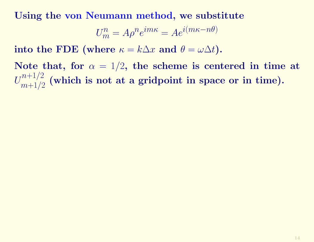
Using the von Neumann method, we substitute

Unm = Aρneimκ = Aei(mκ−nθ)

into the FDE (where κ = k∆x and θ = ω∆t).

14




Note that, for α = 1/2, the scheme is centered in time at

Un+1/2m+1/2 (which is not at a gridpoint in space or in time).

14






We multiply by e−iκ/2 and obtain the amplification factor

ρ =cos κ

2 − i2µα sin κ2

cos κ2 + i2µ(1− α) sin κ

2=

1− i2µα tan κ2

1 + i2µ(1− α) tan κ2

14







ρ =cos κ



2=

1− i2µα tan κ2

1 + i2µ(1− α) tan κ2

Thus, the squared modulus of the amplification factor is

|ρ|2 =1 + 4µ2α2 tan2 κ

2

1 + 4µ2(1− α)2 tan2 κ2

14







ρ =cos κ



2=

1− i2µα tan κ2

1 + i2µ(1− α) tan κ2

Thus, the squared modulus of the amplification factor is

|ρ|2 =1 + 4µ2α2 tan2 κ

2

1 + 4µ2(1− α)2 tan2 κ2

This implies ρ ≤ 1 if α ≤ 0.5, i.e., if the new values are givenat least as much weight as the old values.

14

Again,

|ρ|2 =1 + 4µ2α2 tan2 κ

2

1 + 4µ2(1− α)2 tan2 κ2

For α ≤ 0.5, there is no restriction on the size of ∆t!

15

Again,

|ρ|2 =1 + 4µ2α2 tan2 κ

2

1 + 4µ2(1− α)2 tan2 κ2


Absolute stability — independent of the Courant number— is typical of implicit time schemes.

15

Again,

|ρ|2 =1 + 4µ2α2 tan2 κ

2

1 + 4µ2(1− α)2 tan2 κ2



In an implicit scheme, a point at the new time level is in-fluenced by all the values at the new level, which avoidsextrapolation, and is absolutely stable.

15

Again,

|ρ|2 =1 + 4µ2α2 tan2 κ

2

1 + 4µ2(1− α)2 tan2 κ2




Note also that if α < 0.5 the implicit time scheme reducesthe amplitude of the solution: it is an example of a dampingscheme.

15

Again,

|ρ|2 =1 + 4µ2α2 tan2 κ

2

1 + 4µ2(1− α)2 tan2 κ2




Note also that if α < 0.5 the implicit time scheme reducesthe amplitude of the solution: it is an example of a dampingscheme.

This property is useful for solving problems such as spuri-ously growing mountain waves in semi-Lagrangian schemes.

15

Schematic of an implicit scheme. Note that with the implicit scheme

there is no extrapolation.

16

Summary IIf we consider a marching equation

dU

dt= F (U)

explicit methods such as the forward scheme

Un+1 − Un

∆t= F (Un)

or the leapfrog scheme

Un+1 − Un−1

2∆t= F (Un)

are either

• Conditionally stable, or

• Absolutely unstable.

17

Summary IIA fully implicit scheme

Un+1 − Un

∆t= F (Un+1)

and a centered implicit scheme

Un+1 − Un

∆t= F

(Un + Un+1

2

)

are absolutely stable.

The latter scheme is attractive because it is centered intime, and it can be written with centered space differences,which makes it second order in space and in time.

As these schemes have only two time levels,they have no computational mode.

18

Break here

19

The Crank-Nicholson SchemeThe Crank-Nicholson Scheme is centered in both time andspace.

20


It has good stability and accuracy properties. It is secondorder accurate and unconditionally stable.

20



Two forms of the Crank-Nicholson scheme for the advectionscheme are commonly used:

• The four-point C-N scheme:

12

[Un+1

m −Unm

∆t +Un+1

m+1−Unm+1

∆t

]+ c

2

[Un+1

m+1−Un+1m

∆x +Un

m+1−Unm

∆x

]= 0

20



Two forms of the Crank-Nicholson scheme for the advectionscheme are commonly used:

• The four-point C-N scheme:

12

[Un+1

m −Unm

∆t +Un+1

m+1−Unm+1

∆t

]+ c

2

[Un+1

m+1−Un+1m

∆x +Un

m+1−Unm

∆x

]= 0

• The six-point C-N scheme:

Un+1m − Un

m

∆t+

c

2

[Un+1

m+1 − Un+1m−1

2∆x+

Unm+1 − Un

m−1

2∆x

]= 0

20

Domain of Dependence of Implicit Scheme

*--------*--------*--------•--------*--------*--------* n+1| | | • | | | || | •| | | | |*--------*--•-----*--------*--------*--------*--------* n| | | | | | |m-3 m-2 m-1 m m+1 m+2 m+3

21


*--------*--------*--------•--------*--------*--------* n+1| | | • | | | || | •| | | | |*--------*--•-----*--------*--------*--------*--------* n| | | | | | |m-3 m-2 m-1 m m+1 m+2 m+3

The line of bullets (•) represents a parcel trajectory.

The value at the point m∆x at time (n + 1)∆t depends onall the points denoted by red asterisks (*).

21


*--------*--------*--------•--------*--------*--------* n+1| | | • | | | || | •| | | | |*--------*--•-----*--------*--------*--------*--------* n| | | | | | |m-3 m-2 m-1 m m+1 m+2 m+3

The line of bullets (•) represents a parcel trajectory.

The value at the point m∆x at time (n + 1)∆t depends onall the points denoted by red asterisks (*).

Thus, the computational domain of dependence surroundsthe physical domain of dependence.

This is a necessary condition for a stable scheme.

21

Implicit Schemes & Linear SystemsAll implicit schemes also have a significant disadvantage.

22


Since Un+1 appears on the left- and on the right-hand sides,the solution for Un+1, requires the solution of a system ofequations.

22



If it involves only tridiagonal systems, this is not an obstacle,because there are fast methods to solve them.

22




There are also methods, such as fractional steps (with eachspatial direction solved successively), where one space di-mension is considered at a time.

22




There are also methods, such as fractional steps (with eachspatial direction solved successively), where one space di-mension is considered at a time.

These so-called ADI (alternating direction implicit) schemesallow large time steps without a large additional computa-tional cost.

22

Example of a Linear System.The 1-D advection equation on a periodic domain is

∂u

∂t+ c

∂u

∂x= 0 u(L, t) = u(0, t)

23


∂u

∂t+ c

∂u

∂x= 0 u(L, t) = u(0, t)

The implicit scheme (six-point Crank-Nicholson) scheme is

Un+1m − Un

m

∆t+

c

2

[Un+1

m+1 − Un+1m−1

2∆x+

Unm+1 − Un

m−1

2∆x

]= 0

23


∂u

∂t+ c

∂u

∂x= 0 u(L, t) = u(0, t)

The implicit scheme (six-point Crank-Nicholson) scheme is

Un+1m − Un

m

∆t+

c

2

[Un+1

m+1 − Un+1m−1

2∆x+

Unm+1 − Un

m−1

2∆x

]= 0

We can write this in matrix form (with µ = c∆t/4∆x)

1 +µ 0 . . . −µ−µ 1 +µ . . . 00 −µ 1 . . . 0... ... ... . . . ...

+µ 0 0 . . . 1

Un+10

Un+11

Un+12...

Un+1M−1

=

1 −µ 0 . . . +µ+µ 1 −µ . . . 00 +µ 1 . . . 0... ... ... . . . ...−µ 0 0 . . . 1

Un0

Un1

Un2...

UnM−1

where xM = M∆x and UnM = Un

0 for all n.

23

Symbolically, the equation may be written

M1Un+1 = M2U

n

24


M1Un+1 = M2U

n

The formal solution of this is

Un+1 = M−11 M2U

n

24


M1Un+1 = M2U

n


Un+1 = M−11 M2U

n

However, this requires the inversion of an M ×M matrix.There are much better ways to solve it.

24


M1Un+1 = M2U

n


Un+1 = M−11 M2U

n


The matrix M1 is periodic tri-diagonal. There are very effi-cient numerical methods of inverting a system with such amatrix.

24


M1Un+1 = M2U

n


Un+1 = M−11 M2U

n



The non-periodic problem, with Un0 and Un

M given, resultsin a slightly different matrix, also tri-diagonal.

24


M1Un+1 = M2U

n


Un+1 = M−11 M2U

n



The non-periodic problem, with Un0 and Un

M given, resultsin a slightly different matrix, also tri-diagonal.

If the non-linear terms are treated implicitly, we must solvea nonlinear algebraic system every time step.

This is normally impractical.

24

The possibility of using a time step with a Courant numbermuch larger than 1 in an implicit scheme does not guaranteethat we will obtain accurate results economically.

25


The implicit scheme maintains stability by slowing down thesolutions, so that the waves satisfy the CFL condition.

We saw this clearly in the analysis of the six-point Crank-Nicholson scheme.

25




For this reason, implicit schemes are useful for those modesthat are very fast but of little meteorological importance.

25





We will next consider schemes in which the gravity waveterms are implicit while the remaining terms are explicit.

These semi-implicit schemes are of crucial importance inmodern NWP.

& & &

25





We will next consider schemes in which the gravity waveterms are implicit while the remaining terms are explicit.

These semi-implicit schemes are of crucial importance inmodern NWP.

& & &

Exercise: See Notes and Exercises, Kalnay, pp. 87–88.

25

Conclusion of §3.2.4

26

Documents

3.2 .4 The leapf ro g sc he m e is st able fo r the osci