By:

Prof. Taieb Ali Aouak Dr.Abeer beagan

Dr. Saad Al-qahtany MS. Hind Alrushud

Mr. Mansour Alharthi

CHEM336

PHYSICAL CHEMISTRY OF SOLUTIONS (Laboratory)

Table of content

Laboratory Safety and Guidelines

Experiment No (1) Determination of partial molar volume

Experiment No (2-3) Raoult's Law for Ideal Solutions

Experiment No (4) Ionization and Electrolyte Behavior

Experiment No (5) Temperature-Composition Diagram of a Binary Mixture

Experiment No (6) phase diagram for two partially miscible liquids

Experiment No (7) Cooling curves for Pure substances

Experiment No (8) Determination of the binary solid-liquid diagram for (Naphthalene

and α-Naphthol)

Course grades distribution:

The total score of the practical part is 30 points, distributed as follows:

1. Attendance and reports ( 10 points)

2. First exam( 5 points )

3. Final exam ( 15 points)

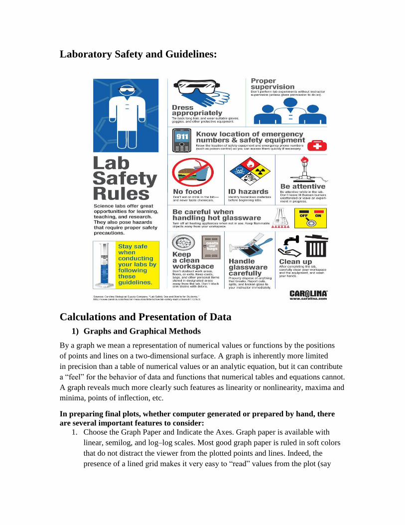
Laboratory Safety and Guidelines:

Calculations and Presentation of Data

1) Graphs and Graphical Methods

By a graph we mean a representation of numerical values or functions by the positions

of points and lines on a two-dimensional surface. A graph is inherently more limited

in precision than a table of numerical values or an analytic equation, but it can contribute

a “feel” for the behavior of data and functions that numerical tables and equations cannot.

A graph reveals much more clearly such features as linearity or nonlinearity, maxima and

minima, points of inflection, etc.

In preparing final plots, whether computer generated or prepared by hand, there

are several important features to consider:

1. Choose the Graph Paper and Indicate the Axes. Graph paper is available with

linear, semilog, and log–log scales. Most good graph paper is ruled in soft colors

that do not distract the viewer from the plotted points and lines. Indeed, the

presence of a lined grid makes it very easy to “read” values from the plot (say

interpolate between points to find y at some desired value of x ). In choosing the

horizontal and vertical scales to be used, attention should be paid to making a

commensurate choice where a major scale division corresponds to an attractive

integral number of the smallest divisions.

2. Use Clear Scale Labels. Choose suitable scale divisions with longer tick marks

used for the major values along a scale that will be labeled with the appropriate

numerical values. Under the scale numbers for the independent variable, enter the

scale label, stating the quantity that is varying and its units: e.g., T(K) for absolute

temperature in kelvin. To avoid scale numbers that are too large or too small for

convenient use, multiply the quantity by a power of 10.

3. Distinguish Smooth Curves. If your plot contains several empirical smooth curves

or several theoretical curves, it is wise to distinguish them by using dashed and

dash–dot curves as well as solid lines.

4. Add a Legend. Somewhere on the figure (if possible, at the bottom) enter a legend

with an identifying figure number. The legend should state the contents of the

figure, identify the symbols and line types used, and provide any needed

information that will not be provided in the text of the document in which the

figure will appear.

5. Plot the Points and Draw the Lines and Curves. Using a sharp, hard pencil, plot

the experimental points as small dots, as accurately as possible. Draw small

circles (or squares, triangles, etc.) of uniform size (2 or 3 mm) around the points

in ink to give them greater visibility.

Experiment No (1)

Determination of partial molar volume Objective:

To calculate partial molar volumes of water-ethanol mixtures as a function of

concentration from densities measured with a pycnometer.

Theory:

the extensive properties (such as volume, free energy, enthalpy, etc.) of a solution are

not additive properties of its components. For example, when one mixes 1 mole of H2O

(which has a molar volume of 18 cm3) with a large quantity of ethanol, the volume

increase observed is not 18 cm3. The surrounding of a molecule is very important in

determining how much volume it will occupy, how much energy it will have, etc. So,

H2O molecules surrounded by other H2O molecules behaves quite differently from H2O

molecules surrounded by ethanol molecules.

Partial molar volume �̅�i: The change in molar volume V when one mole of Ai is added

to an “infinitely large” sample at constant T and P.

V̅A = (𝜕𝑣𝑇

𝜕𝑛𝐴)

𝑇,𝑃,𝑛𝐵

(1)

Equation 1 gives the partial molar volume of the component A for a binary system with

components A and B. Where V is the total volume, nA is the number of moles of A.

Experimental Determination of Partial Molar Volume using tangent-

intercept method

The total volume of the binary solution composed of A (“solvent”) and B (“solute”)

becomes

VT = nA V̅A + nB V̅B (2)

It is convenient to express this on a per-mole basis, dividing through by the total number

of moles (nA + nB) to obtain the equivalent equation in terms of mole fraction XB (with

XA = 1 – XB)

V̅ = XA V̅A + XB V̅B = (1- XB ) V̅̅ ̅̅A + XB V̅B = V̅A + XB (V̅B - V̅A ) (3)

As shown by the final equation on the right, the equation for V̅ = V̅ (XB) is that of a

straight with slope

ⅆV̅

ⅆXB= V̅ 𝐵 − V̅A (4)

And intercept V̅A. The graph below shows the plotted behavior of V(XB) (solid line) from

V̅A0 (at XB = 0) to V̅B

0 (at XB =1), with its corresponding tangent line (dashed) at the

concentration of interest (circle, dotted line). As shown in the graph, extrapolation of the

tangent line to the axes yields V̅A (on the left) and V̅B (on the right). The extrapolated-

tangent construction therefore makes it easy to read off the partial molar volumes V̅A, V̅B

at any desired concentration XB.

Figure 1

Chemicals and Apparatus Ethanol, distilled water, 25 ml pycnometer, balance, graduated cylinder, flask…etc.

Procedure

Prepare a series of solutions by weight containing ethanol and water 20, 40, 60,

80-wt% of ethanol.

Determine the density of each solution at room temperature using the following

procedure:

Determine the weight of previously oven-dried and cooled pycnometer

(m1).

Fill up the empty pycnometer with distilled water, making sure that the

water level in the pycnometer reaches the top of the capillary and is free of

air bubbles.

Determine the weight of the pycnometer, which is filled with water

m(Pyc+water). When doing this, make sure that the outside of the pycnometer

is completely dry.

Given the density of water at ambient temperature, ρ = 0.997 g/ml

calculate the volume of pycnometer using equation 5.

V(Pyc) = m2 −m1

ρ (5)

Subsequently weigh the pycnometer, which is filled with different

mixtures of ethanol and water (m2) then calculate the densities of these

solutions.

Calculate the specific volume d-1 (= reciprocal density ml/g) for each

solution and plot the specific volume versus mole fraction of ethanol for

each solution.

Draw a smooth curve through all points.

Draw tangent lines to this curve at different concentrations and determine

the y-intercepts of these lines on X= 0 and X= 1 the former is the specific

volume of water and the latter is the specific volume of ethanol.

Calculate the partial molar volume of each component using equation 6.

V̅ = Mwt d-1 (6)

Mwt of ethanol = 46.07 g/mol and Mwt of water = 18.015 g/mol

Draw two “partial molar volume versus mole fraction” curves for water

and ethanol and determine the partial molar volumes for the components

at X(EtOH) = 0.2, 0.4, 0.6, and 0.8.

Calculate the total volume of each solution using equation (2).

Report Students' Names:

Object:

m 1 (empty Pyc) = m (Pyc + water) = V (pyc) =

1. Plot the specific volume versus mole fraction of ethanol for each solution.

2. Plot two “partial molar volume versus mole fraction” curves for water and ethanol

W% m = m2 – m1 d-1 V̅ (EtOH) V̅ (water) VT

0

20

40

60

80

100

Experiment No (2-3)

Raoult's Law for Ideal Solutions

Object: to examine how two different mixtures (hexane-heptane and hexane-

isopropanol) obey Raoult’s law.

Introduction: The concept of an ideal solution is important in the development of an

understanding of the properties of real solutions. In a liquid solution, molecules are in

intimate contact with one another so that the question of ideality is determined by the

nature of the intermolecular forces. Suppose a solution is formed by mixing two liquids,

A and B. Then, the solution is ideal if the intermolecular forces between A and B

molecules are no different from those between A and A, or B and B molecules. An

indication of whether or not the condition for ideality is met is obtained from the vapor

pressure of the solution. At a given temperature, the vapor pressure of a pure liquid is a

measure of the ability of molecules to escape from the liquid to the gas phase. By

studying the vapor pressure of a solution as a function of its composition at constant

temperature one may assess the solution’s ideality or its degree of departure from

ideality. For an ideal solution, the tendency of molecule A to escape is proportional to its

mole fraction, that is, to its concentration expressed in terms of the fraction of molecules

which are of type A. The proportionality constant must be the vapor pressure of pure

component A because this vapor pressure is reached when the mole fraction is unity. This

result is Raoult’s law, which is expressed mathematically as

PA = PA XA (1)

Similarly, for the other component B,

PB = PB XB (2)

The total pressure above the solution includes both components; the solvent and the

solute unless the solute is nonvolatile.

PT = PA XA + PB XB (3)

When a solution is boiling, its vapor pressure (PT) is equal to the current atmospheric

pressure. To assess the solution’s ideality, we need to measure both P(solvent) and

P(solute) at the boiling temperatures. Although it is relatively straightforward to

Figure 2

determine the composition of the solution phase, measuring the composition of the vapor

phase is a bit more difficult. However, it’s possible to calculate vapor pressure of a pure

liquid (The proportionality constant in Raoult’s law) using the Clausius-Clapeyron

equation.

Clausius-Clapeyron equation (4), although only approximate, provides a useful tool for

estimating the vapor pressure changes of a pure liquid as a function of temperature.

ln (𝑃 𝑣𝑎𝑝

P) =

− ∆𝐻 𝑣𝑎𝑝 (T,P)

𝑅 (

1

𝑇(𝐾)−

1

𝑇(𝐾)𝑏𝑝) (4)

P Vap = 𝑒− ∆𝐻 𝑣𝑎𝑝

𝑅 (

1

𝑇(𝐾) −

1

𝑇(𝐾)𝑏𝑝)

Where P is the atmospheric pressure which is equal to 1, P is the vapor pressure at some

absolute temperature T, R is the universal gas constant and Tbp is pure liquid’s normal

boiling point. ∆𝐻 𝑣𝑎𝑝 (T, P) is the heat of vaporization, it is function in temperature and

pressure, but it is nearly constant over the usual effective range of T and P variations, we

assume that it can be replaced by the fixed molar enthalpy of vaporization ΔH vap for

standard state conditions (e.g., 25 C, 1 atm).

Condenser is open here; do not cork!

Warm water out

Cold water in

30C and beyond visible

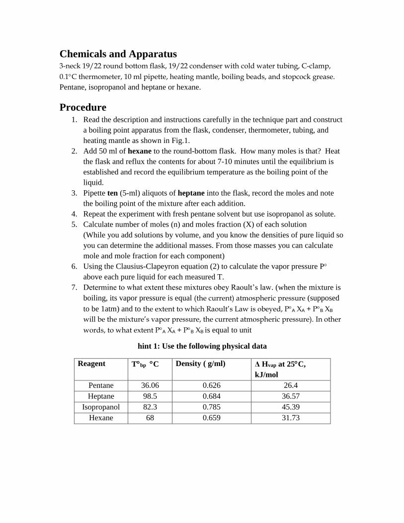
Chemicals and Apparatus 3-neck 19/22 round bottom flask, 19/22 condenser with cold water tubing, C-clamp,

0.1C thermometer, 10 ml pipette, heating mantle, boiling beads, and stopcock grease.

Pentane, isopropanol and heptane or hexane.

Procedure 1. Read the description and instructions carefully in the technique part and construct

a boiling point apparatus from the flask, condenser, thermometer, tubing, and

heating mantle as shown in Fig.1.

2. Add 50 ml of hexane to the round-bottom flask. How many moles is that? Heat

the flask and reflux the contents for about 7-10 minutes until the equilibrium is

established and record the equilibrium temperature as the boiling point of the

liquid.

3. Pipette ten (5-ml) aliquots of heptane into the flask, record the moles and note

the boiling point of the mixture after each addition.

4. Repeat the experiment with fresh pentane solvent but use isopropanol as solute.

5. Calculate number of moles (n) and moles fraction (X) of each solution

(While you add solutions by volume, and you know the densities of pure liquid so

you can determine the additional masses. From those masses you can calculate

mole and mole fraction for each component)

6. Using the Clausius-Clapeyron equation (2) to calculate the vapor pressure P

above each pure liquid for each measured T.

7. Determine to what extent these mixtures obey Raoult’s law. (when the mixture is

boiling, its vapor pressure is equal (the current) atmospheric pressure (supposed

to be 1atm) and to the extent to which Raoult’s Law is obeyed, PA XA + PB XB

will be the mixture’s vapor pressure, the current atmospheric pressure). In other

words, to what extent PA XA + PB XB is equal to unit

hint 1: Use the following physical data

Reagent Tbp C Density ( g/ml) Δ Hvap at 25C,

kJ/mol

Pentane 36.06 0.626 26.4

Heptane 98.5 0.684 36.57

Isopropanol 82.3 0.785 45.39

Hexane 68 0.659 31.73

Technique: We will use a procedure called reflux. As the solution boils, cool water in

the condenser will condense the vapor and the liquid will re-enter the flask. You should

smell little or no vapor during the experiment.

Using a clamp, attach a round-bottom flask with a condenser to a burette stand. The flask

should rest on a heating mantle on a heat-resistant surface. Drop a few boiling beads into

the flask. Smear a small amount of stopcock grease on the tip of the thermometer to make

it slide more easily into its cork. Insert the thermometer into the flask's side arm so that it

does not touch the flask's sides or bottom. Be sure you can read the thermometer from

30C. The bulb should be inside the vapor as the solution boils; you’ll see condensation

forming on it; that ensures it is measuring the boiling point accurately. The thermometer

should not be IN the liquid!

Attach tubing snugly to the condenser's nozzles. Attach the bottom tube to a cold water

tap and allow the other tube to go down the drain. Start the cold water flowing before the

addition of the volatile solvent.

Plug in the heating mantle and adjust the cooling water to ensure that the condenser stays

cool enough to condense the solvent below its midpoint. As the solvent comes to a rolling

boil, unplug the mantle. It will stay hot for quite some time! The flask will also be hot.

With the “condensation ring” still visible in the condenser, measure the boiling

temperature. Record the current atmospheric pressure, since it is equal to the vapor

pressure above the boiling mixture. The thermometer should be wet; in other words, vapor

should condense on it during the experiment. (But don’t immerse it.)

Add each solute aliquot (means a measured amount) from the 5-ml pipette by dropping it

straight down the condenser tube. The boiling may stop simply because the solute is at

room temperature, but it will most likely resume as the heat from the (still unplugged)

mantle continues warming the mixture. If boiling does not resume with sufficient vigor to

make a condensation ring obvious, plug in the mantle briefly. If the condensation ring

becomes too high, turn on more cold water. Be careful when you do this -- the tubing

might pop off the condenser! As a last resort if the condensation ring threatens to rise out

of the condenser, raise the glassware up out of the mantle by sliding its clamp.

Allow the temperature reading to come to its equilibrium after each addition to obtain an

accurate reading of the mixture's boiling point. Do not add so much solute that the boiling

point approaches the thermometer’s maximum temperature!

At the end of the experiment, turn off and remove the heating mantle (be careful, it's hot!)to

permit the flask and mixture to cool to a comfortable temperature. Discard these reagents

in the non-halogenated organic waste bottle. Also turn off the water, drain the condenser

into the sink, and clean and return all borrowed equipment. Be sure the heating mantle has

cooled to room temperature.

Report Students' names:

Object:

Report hints: include your data and graphs in your Results section. In the Discussion,

describe the influence of any non-idealities on your results. Is Raoult's Law obeyed? Why

or why not? Determine the extent to which you might ignore the vapor pressure of the

solutes in both experiments; in other words, what would the solute vapor pressures be near

the solvent's boiling point? Are they negligible? Use the Clausius-Clapeyron equation in

your answer.

Results

Mixture 1

V(Hexane)

ml

V(Heptane)

ml

m(Hexane) m(Heptane) n(Hexane) n(Heptane) X(Hexane) X(Heptane)

50 0.00

50 5

50 10

50 15

50 20

50 25

50 30

50 35

50 40

50 45

50 50

X(Hexane) T P(hexane) P(Heptane) PT

Mixture 2

V(hexane)

ml

V(isopropanol)

ml

m(hexane) m(isopropanol) n(hexane) n(isopropanol) X(hexane) X(isopropa

nol)

50 0.00

50 5

50 10

50 15

50 20

50 25

50 30

50 35

50 40

50 45

50 50

X(Hexane) T P(hexane) P( isopropanol) PT

Discussion

Experiment No (4)

Ionization and Electrolyte Behavior

Objects: In this experiment, you will

• Use a Conductivity Probe to measure the conductivity of solutions.

• Investigate the conductivity of solutions resulting from compounds that dissociate to

produce different numbers of ions.

Theory: The size of the conductivity value depends on the ability of the aqueous

solution to conduct electricity. Strong electrolytes produce large numbers of ions, which

results in high conductivity values. Weak electrolytes result in low conductivity, and non-

electrolytes should result in no conductivity. In this experiment, you will observe several

factors that determine whether or not a solution conducts, and if so, the relative

magnitude of the conductivity. Thus, this simple experiment allows you to learn a great

deal about different compounds and their resulting solutions. Keep in mind that you will

be encountering three types of compounds and aqueous solutions:

Ionic Compounds:

These are usually strong electrolytes and can be expected to 100% dissociate in aqueous

solution.

Molecular Compounds:

These are usually non-electrolytes. They do not dissociate to form ions. Resulting

solutions do

not conduct electricity.

Molecular Acids

These molecules can partially or wholly dissociate, depending on their strength.

Chemical and apparatus:

A list of substances to be tested is given on the report sheet. Your instructor may do this

experiment as a demonstration or individual conductivity meters may be given.

Procedure:

1. In a clean-dry beaker, test the conductivity of different substances and solutions

by following the table in your report using the conductivity meter.

2. Answer the questions below the table.

Report of experiment (4)

Students' Names:

Object:

Solution Conductivity (µS/cm)

H2O distilled

Glucose (1M)

NaCl (1M)

NaCl (2M)

NaCl(1M) at 60 C°

H2SO4 (1M)

Answer the following questions:

1. Why did the conductivity increase in (2M) NaCl solution than (1M) NaCl

solution?

2. Why does glucose solution consider as a non-electrolytes solution?

3. When heat was applied in (1M) NaCl solution, why the conductivity was

increased?

4. Why H2SO4 solution is the strongest electrolytes in the list that was

given?

Experiment No (5) Temperature-Composition Diagram of a Binary Mixture

Objects:

The aim of this experiment is to:

1. Study and draw the temperature-composition diagram for ethanol- water solution.

2. Determine the temperature and composition of the azeotrope.

Theory: Distillation is one of the most useful methods for the separation and

purification of liquids. There are many types of distillation such as simple distillation,

fractional distillation, and steam distillation. The difference in boiling points between the

compounds is what determines what type should be used. In the case of non-ideal

solutions, it might not be possible to separate compounds completely. The systems that

are impossible to separate completely are known as azeotropes (azeotrope = not changing

composition when boiling). For example about this case is the separation of ethanol-

water solution.

Chemicals and Apparatus

Distillation Setup: Thermometer, 250-ml round bottom flask, fractional column,

condenser, receiver Elbow, 250 mL- graduated cylinder, Flask heater, rubber adapter,

grains of pumice, mantle, ethanol, distillated water.

Procedure

1. Prepare ethanol solutions with 40, 60, 80, and 95%. Of concentration.

2. Setup the distillation apparatus as showing below :

3. In the 250-ml round bottom flask add 100 ml of 40% ethanol solution and some

grains of pumice.

4. Turn on the mantle hot plate (do not apply high temperature).

5. The solution will start to boil and evaporate and then the resulting steam will

condense and fall in the graduated cylinder.

6. When the first drop falls, record the boiling and the evaporation temperature in

the results table.

7. Repeat the same steps for other solutions.

Calculation

1. Plot T versus x (W %) using your results.

2. Draw smooth curves through the points obtained from boiling temperatures and

through the points obtained from evaporation temperatures.

3. Label all the phases present on the graph.

4. Determine the azeotropic composition and its boiling point from your graph.

Report Students' Names:

Object:

W % Tb

(boiling temperatures) Tv

(evaporation temperatures)

0

40

60

80

95

99

100

From the graph answer the following questions :

1- In what concentration does the azeotropic occur?

2- What is the boiling point for the azeotropic ?

Experiment No (6)

phase diagram for two partially miscible liquids

Object: to construct a phase diagram of two immiscible liquids (aniline-heptane

system) and find out the critical solution temperature of this system.

Theory: When two partially miscible liquids are mixed and shaken together, we get

two solutions of different composition. For example, on shaking aniline and heptane, we

get two layers; the upper layer is a solution of heptane in aniline and the lower layer is a

solution of aniline in heptane. At a fixed temperature, the composition of each solution is

fixed and both the solutions are in equilibrium. The composition of the two layers

(phases) at equilibrium varies with the temperature. Raising the temperature increasing

the miscibility of the two solutions. Above a particular temperature, such solutions are

completely miscible in all proportions. This temperature is known as Upper Critical

Solution Temperature. Figure (1) shows the temperature-composition diagram for a

mixture of A and B. The region below the curve corresponds to the compositions and

temperatures at which the liquids are partially miscible. The upper critical temperature Tc

is the highest temperature at which phase separation occurs and above Tc the two

solutions are fully miscible.

Figure 3 The temperature composition diagram of a mixture of A and B.

Chemical and Apparatus: Aniline, heptane, water bath, thermometer,

beaker and pipette.

Procedure:

1. 10 ml of aniline was measured into a test tube and then 1 ml of heptane added to

it.

2. The two-phase solution was then heated in a water bath until a single-phase

solution was formed.

3. The temperature at which the single-phase formed was measured and recorded.

4. The volume of aniline was kept varying with respect to heptane as shown in the

below table.

5. A curve is plotted with temperature as ordinate against mass fraction of aniline as

abscissa. The maxima of the solubility curve will give the critical solution

temperature.

Density of heptane = 0.706 g/ml, density of aniline = 1.023 g/ml.

Mass = density × volume.

Mass fraction = 𝑚𝑎𝑠𝑠 𝑜𝑓 𝑎𝑛𝑖𝑙𝑖𝑛𝑒

𝑚𝑎𝑠𝑠 𝑜𝑓 𝑎𝑛𝑖𝑙𝑖𝑛𝑒+𝑚𝑎𝑠𝑠 𝑜𝑓 ℎ𝑒𝑝𝑡𝑎𝑛𝑒

Precautions; Aniline is toxic and can be absorbed by the skin, care must be taken not to

spill.

Report

Students' Names:

Object:

Table of Results:

Vol. of aniline Vol. of heptane Temperature Mass frac. of aniline.

10 1

9 2

8 3

7 4

6 5

5 6

4 7

3 8

2 9

1 10

Discussion:

Experiment No (7)

Cooling curves for Pure substances

Object:

1- To draw cooling curves for pure substances (Naphthalene, α-Naphthol) and find

their melting points from the curve.

Theory:

A cooling curve for a substance is a curve between temperature and time of cooling. It is

started when the entire mass is liquid and is continued till it is completely solidified. The

curve will be continuous, as long as there is no transition or change of phase. At a certain

temperature, the liquid begins to solidify and heat is found to be liberated during this

phase change of liquid to solid. This method is known as thermal analysis. Due to this

liberation of heat the cooling curve (Fig.1) becomes discontinuous. The cooling curve

ABCD consists of three parts.

1. AB, which corresponds to the cooling of the liquid. At temperature T1, the liquid

begins to solidify.

2. BC, which corresponds to the separation of the solid. The solid is formed at a rate

just sufficient to counterbalance the heat loss by radiation and hence the

temperature remains constant. At time t, the liquid is completely converted into

solid. This steady temperature is the melting point of the substance.

3. CD, which corresponds to the cooling of the solid phase of the substance.

Note; The melting or freezing temperature is the temperature at which the solid

and liquid phases of a substance can exist in equilibrium. Like any equilibrium

state, the chemical potential of a substance is the same throughout a sample.

Regardless of how many phases are present.

Chemicals and Apparatus Naphthalene, α-Naphthol, Boiling tube, 1-L beaker, Thermometer (0-100˚C), hot plate,

Stop watch, Clamp, stand and boss.

Procedure 1. Put about 800 ml water into the beaker and heat it on the hot plate until the water

starts to boil.

2. In a boiling tube put 1 g of naphthalene, fit a thermometer in this tube then place

it in a boiling water bath, as shown in Fig 2.

3. Shake gently with the thermometer until the substance melts completely.

4. Remove The beaker from the hot plate, keep the tube in the beaker and record the

temperature every 30 sec, (If the rate of cooling is slow, observe reading after a

minute) until it becomes constant and the whole mass solidifies (note at which

temperature you see the solid start to melt).

5. Plot the cooling curve between temperature (ordinate) and time (abscissa) and

note the melting temperature of naphthalene which is characterized by the

temperature of the plateau (stability of temperature with time).

6. Repeat experiment with 1 g of α-Naphthol and determine its melting temperature.

Report

Students' Names:

Object:

Time Temperature Time Temperature

Plot the variation of the temperature as a function of time and determine the

following:

Melting point of Naphthalene = Melting point of α-Naphthol =

Q) Why the temperature remains constant during a transformation from one state

to another state?

Experiment No (8) Determination of the binary solid-liquid diagram for (Naphthalene and α-Naphthol)

Object: To draw a phase diagram for Naphthalene and α-Naphthol and from it find

the eutectic temperature of the binary system.

Theory: If a mixture of two components A and B (melting point of A is higher than that

of B) is melted and cooled and if the percentage of A is higher than that of B in the

mixture, then it is seen that the melting point of A will be lowered due to the presence of

B. At a certain temperature, known as Transition Temperature, solid A will crystallize

earlier, leaving the liquid richer in B. After some more cooling, the composition of the

liquid will reach a ratio of A to B so as to allow the separation of A and B simultaneously

in the crystalline form. Thus, that temperature at which the two solids A and B are in

equilibrium with the solution is known as Eutectic Temperature (Greek: eutectic = easy

melting).

Figure (1) depicts the cooling curve of a mixture of two components A and B (Notice; the

shape is not like a cooling curve of pure substance). The first break in the curve occurs at

B1 where one of the components, begins to solidify. During this solidification process,

heat is liberated, and the temperature falls more slowly. It is to be noted that the

temperature does not remain constant because the composition of the mixture (amount of

A: amount of B) is changing continuously whereby the temperature of solidification

correspondingly changes. At a certain temperature T2, known as Eutectic Temperature,

the remaining liquid solidifies, both the components A and B crystallize out

simultaneously.

Figure 4

If we draw cooling curves for several mixtures of A and B and plot the corresponding

Transition Temperatures as ordinate against composition (Mole fraction) as abscissa,

we get a phase diagram [fig. (2)], from which we can find the melting points of the two

components as well as the Eutectic Temperature of the system.

5

Chemicals and Apparatus

Naphthalene, α-Naphthol, Boiling tube, 1-L beaker, Thermometer (0-100˚C), hot plate,

stopwatch, Clamp, stand and boss.

Procedure

1. Put about 800 ml water into the beaker and heat it on the hot plate until the water

starts to boil.

2. Prepare the following mixtures of Naphthalene and α-Naphthol by weighing them

separately.

Mixture 1 2 3 4 5

Naphthalene 0.2 g 0.4 g 0.5 g 0.7 g 0.9 g

α-Naphthol 0.8 g 0.6 g 0.5 g 0.3 g 0.1 g

3. In a boiling tube put the first mixture, fit a thermometer in this tube then place it

in a boiling water bath. Shake gently with the thermometer until the mixture melts

completely.

4. Remove The beaker from the hot plate, keep the tube in the beaker and record the

temperature every 30 sec, (If the rate of cooling is slow, observe reading after a

minute), until it becomes constant and the whole mass solidifies. (note at which

temperature you see the solid start to melt).

5. Remove the thermometer and pour out the contents of the tube. Wash and dry it

and repeat the above process for the remaining mixture of Naphthalene and α-

Naphthol.

Report

Students' Names:

Object:

Mixture 1 Mixture 2 Mixture 3 Mixture 4 Mixture 5

Temp Time Temp Time Temp Time Temp Time Temp Time

1) Draw a cooling curve for every mixture of Naphthalene and α-Naphthol (time is

taken as abscissa while temperature as ordinate). From the cooling curves, find

the transition temperature for each mixture and tabulate the results as follows:

Mixture Mole fraction of Naphthalene Transition temperature

1 (0.2: 0.8)

2 (0.4: 0.6)

3 (0.5: 0.5)

4 (0.7: 0.3)

5 (0.9:0.1)

2) Draw a curve with transition temperature as ordinate and mole fraction of

naphthalene as abscissa and indicate on this solid-liquid diagram the legend of

different zones (Liquid phase, solid phase, Eutectic point).