Embed Size (px)
Citation preview

349
Bi-Annual Research Journal “BALOCHISTAN REVIEW” ISSN 1810-2174 Balochistan Study Centre,
University of Balochistan, Quetta (Pakistan) VOL. 44, 2019 (SPECIAL EDTION)
Time Series Forecasting with SARIMA Model of Water Outflow of
Indus at Terbela River in Pakistan
Syed Fareed Ullah1
Dr Yasmeen Zahra2
Prof.Dr Ijaz Hussain3
Syed Muhammad Zia ul haq4
Abstract
We have made forecasting of the water outflow of Indus at Terbela
river using the Seasonal Autoregressive Integrated Moving Average
Model. Given Time series has showed seasonality pattern and it is
incorporate in the ARIMA model. The best model is selected among many
candidate models for forecasting the water outflow. The forecast values
are tabulated up to 2020 and graphically shown. The policy maker may
use these predicted values for their purposes.
Keywords: Stationarity, Autoregressive, Moving average, Autoregressive
Moving average, Seasonality, Mean Square Error
_______________
1 Department of Statistics, University of Balochistan, Pakistan
2 Department of Statistics, University of Balochistan, Pakistan
3 Department of Statistics,Quaid e Azam University of Isamabad, Pakistan
4 Department of Geography, Govt. Science College Quetta, Pakistan
350
1. Introduction
The present study is based on time series forecasting of river flows
data of Indus at Terbala river by applying adequate methods like Box-
Jenkins method (Sarjinder Singh, 2003). Autoregressive Integrated
Moving Average (ARIMA) is widely used model for the analysis of
stochastic time series models (Jam, 2013) , (Hipel, 1994) model.
To apply the ARIMA it is assumed that time series is linear and
follows a particular known statistical distribution (Hipel, 1994), (Adhikari
K. & R.K., 2013) Moving Average (MA) (Seymour, Brockwell, & Davis,
1997) and Autoregressive Moving Average (ARMA) (Mills, 2015)
models. For seasonal time series forecasting, Box and Jenkins (Klose,
Pircher, & Sharma, 2004) had proposed a quite successful variation of
ARIMA model, viz. the Seasonal ARIMA (Elganainy & Eldwer, 2018).
ARIMA is most famous and widely used model in time series analysis due
to its flexibility to represent several varieties of time series with simplicity
as well as the associated Box-Jenkins methodology (Since & Model,
2008), (Naveena, Singh, Rathod, & Singh, 2017).
1.1 Background of Study:
After Box-Jenkins, neural systems are taken place as an efficient
technique. In 1940s, the systems of neural nets have its birthplace
(McCulloch, 1943) and (Hebb, 1949) which has been seen into systems of
basic processing method that can be demonstrate/model neurological
action and acquiring inside these systems, individually.

351
1.2 Problem Statement:
The economical procedures based on the forecasting issues for
slight over the improvement of methods. Statistical and Econometrical
methods are generally used the information as a part of overseeing
generation frameworks. These methods have additionally revealed
common application in an variety of other issue ranges. In financial
matters, there are numerous issues which require the utilization of large
panel of time series.
1.3 Significance/Justification of Study:
The recent technique is the way toward utilizing likelihood to
attempt to forecast the probability of specific occasions happening in the
future.
a) Operations management
b) Marketing
c) Finance & Risk management
d) Economics
e) Industrial Process Control Demography:
f) forecast of population
1.4 Objectives of Study
We focus on the real-world problem in the Pakistan Tarbela River.
The objects of this study to fit the Model, identification, estimation and
forecasting as well as forecasting to use SARIMA.

352
1.5 Research Questions:
1. How to identify the model?
2. How to estimate model?
3. How to forecast the model?
1.6 Limitation of Study:
There are some limitations regarding this study because its finding
may not be generalized for the entire Pakistan Tarbela river flows due to
the listed below reasons:
It adopts recent techniques
It is restricted to a specific data
The status of its finding may vary from time to time
2. Literature Review
(Chatfield, 1996) a model is rarely pre-specified but rather is typically
formulated in an iterative, collaborative way using the given time-series
data. Empirically, it established that the more complicated models tend to
give a better fit but forecasts.
(Jones & Smart, 2005) demonstrated that Autoregressive modelling is used
to explore the internal structure of long-term records of nitrate
concentration for five karst springs in the Mendip Hills and found that there
exists significant short term positive autocorrelation at three of the five
springs due to the availability of sufficient nitrate within the soil store to
sustain concentrations in winter revive for several months.
(Cai, Lye, & Khan, 2009) have been provided flood warnings to the
residents living along the various sections of the Humber River Basin, the
Water Resources Management Division (WRMD) of the Department of
353
Environment and Conservation has calculated flow forecasts for this basin
over the years by means of numerous rainfall-runoff models.
(Rbunaru & Cescu, 2013) provided the time series data formed in
both dynamic and time series which differ from other data sets which are
arranged according to the time variable. The important and essential
component of time series are seasonal fluctuations along with trend,
cyclical and random oscillations are seasonal fluctuations. They provided
the suitable method for the analysis of seasonal fluctuations.
(Valipour, Banihabib, Mahmood, & Behbahani, 2013) presented in
their present study of forecasting the inflow of Dez dam reservoir by using
ARMA and ARIMA models and increased the number of parameters to
enhance the accuracy of forecasting. They compared these models with
the static and dynamic ANNs.
(Jam, 2013) has tried to explore the adequate Auto Regressive
Integrated Moving Average model by through Box-Jenkins methodology
to predict the area of mangoes in Pakistan. In this present study time series
data from 1961 to 2009 has been used for forecasting of area of mangoes.
(Merkuryeva & Kornevs, 2014) presented the methods for flood
forecasting and simulation which are applied to a river flood analysis and
risk prediction. They applied different models for different water flow
forecasting and river simulation.
It was the time when the creation of (Box , 1976), ARIMA models,
furthermore called Box–Jenkins models, have been an extremely
understood kind of time course of action models used as a bit of hydro-
logical forecasting the values. For the recent appliances, see for instance
(Maria Castellano , 2004).
354
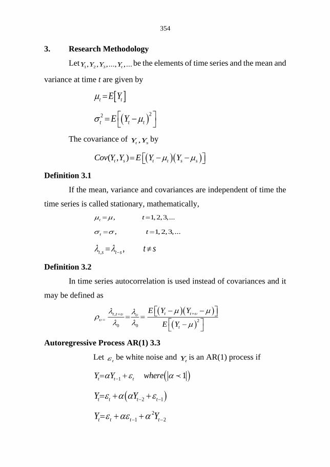
3. Research Methodology
Let1 2 3, , ,..., ,...tY Y Y Y be the elements of time series and the mean and
variance at time t are given by
t tE Y =
( )22
t t tE Y = −
The covariance of ,t sY Y by
( )( )( , )t s t t s sCov Y Y E Y Y = − −
Definition 3.1
If the mean, variance and covariances are independent of time the
time series is called stationary, mathematically,
, 1,2,3,...t t = =
, 1,2,3,...t t = =
, ,t s t s t s −=
Definition 3.2
In time series autocorrelation is used instead of covariances and it
may be defined as
( )( )
( )
,
20 0
t tt t
t
E Y Y
E Y
++
=
− − = = −
Autoregressive Process AR(1) 3.3
Let t be white noise and
tY is an AR(1) process if
( )1 1t t tY Y where −= +
( )2 1t t t tY Y − −= + +
2
1 2t t t tY Y − −= + +

355
( )2
1 3 2t t t t tY Y − − −= + + +
2 3
1 2 3t t t t tY Y − − −= + + +
. . . . .
. . .
. . . . .
2 3
1 2 3 ...t t t t tY − − −= + + + +
0tE Y = ; It is independent of time.
Also, the autocorrelation is
,k t t kE Y Y +=
0 0
i i
k i it i t iE
= =− −
=
2
0
i k i
k i +
==
2 2
0
Infk i i
k i +
==
2
21
k
k k
=
− where
0
kk
=
0,1,2,3,...k
k k = =
0, 1, 2, 3,...k
k k = = which is independent of
time. Thus AR(1) is stationary process.
Notation of Lag Operators 3.4
Consider the time series 1 2 3, , ,..., tY Y Y Y then we define the lag
operator represented by L as given below:

356
( ) 2 3
1 1 2 31 ... p
t t pLY Y if L L L L L −= = − − − − −
Then we may define AR(1) process as follow:
1 1 2 2 3 3 ...t t t t p t p tY Y Y Y Y − − − −= + + + + + where t is
white noise. So, using lag operator, it may be written as
2 3
1 2 3 ... p
t t t t p t tY LY L Y LY L Y = + + + + +
( )2 3
1 2 31 ... p
p t tL L L L Y − − − − − =
( ) t tL Y = where 1
Autoregressive Process AR(2) 3.5
AR(2) process may be written as
1 1 2 2t t t tY Y Y − −= + +
Using lag operators, we have
( )2
1 21 t tL L Y − − =
Also the process may be write as
( )t tY L =
( )2 3
1 2 31 ...t tY L L L = + + + +
Where
( ) ( )1
2 2 3
1 2 1 2 31 1 ...L L L L L −
− − = + + + +
( )( )2 2 3
1 2 1 2 31 1 ... 1L L L L L − − + + + +
Equating coefficients, we have
1
1 1 1 1: 0L − + = =
2 2
2 1 1 2 1 1 1: 0L − + + = = +

357
3 2 3
2 1 1 2 1 1 1 2: 0 2L − + + = = +
1 1 2 2:j
j j jL − −= +
All the weights can be determined recursively.
Autoregressive Process AR(p) 3.6
AR(p) is defined as
1 1 2 2 ...t t t p t p tY Y Y Y − − −− − − − =
( )2 3
1 2 31 ... p
p t tL L L L Y − − − − − =
( ) t tL Y = where
( ) ( )2 3
1 2 31 ... p
pL L L L L = − − − − −
With the following condition of stationarity that can be set out as
follows by writing
( ) ( )( )( ) ( )1 2 31 1 1 ... 1 pL h L h L h L h L = − − − −
1 1,2,3,...,ih for i p=
Alternatively, we may write
1
ih−all lie outside the unit circle.
The autocorrelation will follow a difference equation of the form
( ) 0 1,2,3,...kL for k = =
Which has the solution in the form
1 1 2 2 3 3 ...k k k k
k p pAh A h A h A h = + + + +

358
Moving Average Process MA(1) 3.7
Here an MA(1) process can be defined as
1t t tY −= +
Where t is the white noise
0tE Y =
( )2
1t t tVar Y E − = +
( )2 2 2
t t tVar Y E E = +
( )2 21tVar Y = +
1 1t tE YY −=
( )( )1 1 1 2t t t tE − − −= + +
2
1 1tE − =
2
1 =
So, we have
1 21
=
+
( )( )2 1 2 3t t t tE − − −= + +
2 0 =
Generally, 0 2j for j . So Moving Average process MA(1) is
stationary irrespective of the value of .
Moving Average MA(q) process can be defined in the following
fashion.
1 1 2 2 3 3 ...t t t t t q t qY − − − −= + + + + +

359
0tE Y =
( )2 2 2 2 2
1 2 31 ...t qVar Y = + + + + +
k t t kCov YY −=
( )
1 1 2 2 3 3
1 1 2 2 3 3
1 1 2 2 3 3
...
...
... ...
t t t t k t k
k t k k t k k t k q t qk
t k t k t k t k q k t q
E
− − − −
+ − − + − − + − − −
− − − − − − − − −
+ + + + + + + + + +=
+ + + + + +
( ) 2
1 1 2 2 ...k k k k q q k + + −= + + + + and
k
k
tVar Y
=
Also, for moving average process to be stationary regardless of the
values of the ,s .
( )
( )0
2 2 2 2
1 2 3
,,
1 ...
0 ,
n k
i i ki
k q
k q
k q
−
+=
= + + + + +
Autoregressive Moving Average ARMA(p,q) Process 3.8
It is mixture of AR(p) and MA(q) processes of order p,q and it is
represented as ARMA(p,q) if
1 1 2 2 3 3 1 1 2 2 3 3... ...t t t t t t t t q t qY Y Y Y − − − − − − −= + + + + + + + + +
( ) ( )2 3 2 3
1 2 3 1 2 31 ... 1 ...p q
p t q tL L L L Y L L L L − − − − − = + + + + +
Or ( ) ( )t tL Y L =
Where the polynomials and of degree p and q respectively in
L.

360
Box-Jenkins Methodology 3.9
Box-Jenkins methodology is very famous and widely used method
of univariate time series analysis, which is a hybirid of
the AR and MA models
1 1 2 2 3 3 1 1 2 2 3 3... ...t t t t t t t t q t qY Y Y Y − − − − − − −= + + + + + + + + +
where the terms in the equation have the same meaning as given for the
AR and MA model.
To apply the Box-Jenkins method, it is assumed that the
time series is stationary. If the time series data is non-stationary then Box
and Jenkins recommend differencing one or more times to achieve
stationarity which produces an ARIMA model, where the "I" stands for
"Integrated".
To include the seasonal autoregressive and seasonal moving
average terms, we extends the Box-Jenkins models which may complicate
the notations and mathematics of the model.
Box-Jenkins model commonly includes difference operators,
autoregressive terms, moving average terms, seasonal autoregressive
terms, seasonal difference operators, , and seasonal moving average terms.
The four stages of methodology are:
➢ Identification
➢ Estimation
➢ Diagnostic check on Model adequacy
➢ Forecasting
These steps may be shown by a logic flow diagram as below:

361
Box-Jenkins Methodology stage of Identification 3.9.1
For the implementation of the Box-Jenkins model, the initial first
step is to determine if the series is stationary.
Only the partial autocorrelation function computed from sample is
generally not helpful for identifying the order of the moving average
process. Here are the basic guideline are listed below for the identification
of AR(p) and MA(q) processes.
Box-Jenkins Methodology stage of Estimation 3.9.2

362
The step for the implementation of Box-Jenkins methodology is the
estimating the parameters. Therefore, the parameter estimation is
accomplished using sophisticated and high-quality software program that
successfully implement Box-Jenkins models.
Box-Jenkins Methodology stage of Diagnostics 3.9.3
When some candidate models are listed then next step is to check
diagnostics for Box-Jenkins models. It means that the error term as
assumed to follow the assumptions for a stationary univariate process, That
is residuals should be white noise, that is having a constant mean and
variance. If the residuals satisfy these assumptions, then it is expected that
Box-Jenkins model is a good model for the data and will forecast the time
series better.
Box-Jenkins Methodology stage of Forecasting 3.9.4
When best is selected then it will be used for forecasting.
Seasonal ARIMA Model 3.9.5
If there exists the seasonal trend after k period of then we try to
remove the seasonality from the series and produce a modified time series
which may not be seasonal. After that we apply the Box-Jenkins
methodology of ARIMA model. Mathematically, let tv be the nonseasonal
time series, then the proposed the seasonal ARIMA (SARIMA) model
filter as
( )( ) ( )1D
k k k
k t k tL L Y L v − =
Where
( ) 2 3
1 2 31 ...k k k k Pk
k k k k PkL L L L L = − − − − −
( ) 2 3
1 2 31 ...k k k k Qk
k k k k QkL L L L L = − − − − −

363
Alsotv is the ARIMA(p,d,q) which is the estimated using the
ARIMA model as follow
( )( ) ( )1d
t tL L v L − =
Putting fortv , we have
( )( ) ( )( ) ( ) ( )1 1D D
k k k k k
k k tL L L L L L − − =
Which is SARIMA.
3.1 Research Design:
Appropriate quantitative techniques will be applied for the finding
of this study. The method will be compare to find the adequate and
appropriate technique to forecast the values of the water outflow data.
3.2 Data Collection and analysis
Secondary time series data of water outflow is used from 2015 to
2019 recorded on daily basis. Appropriate and adequate statistical method
have been applied using R, a statistical software.
4. Results and Discussion

364
Figure 4.1:- Time series plot of Water Outflow data
From figure 4.1, it is shown that there is seasonality in the
data as within a year it may be repeated in a similar way. It looks like a
non-stationary time series as the mean and variance are not same with
respect to time. We may note that there is gradual decrease in water
outflow. For more elaboration we have other plots as given below.
Figure 4.2:- The First Difference Plot of Water Outflow
From figure 4.2, it is shown the mean of the given series
becomes the constant with respect to time after taking the first difference
of the series. It can also be seen that there is a seasonal trend the series and
it can be further explore as below:
Figure 4.3:- Seasonal Plot of the Water outflow
365
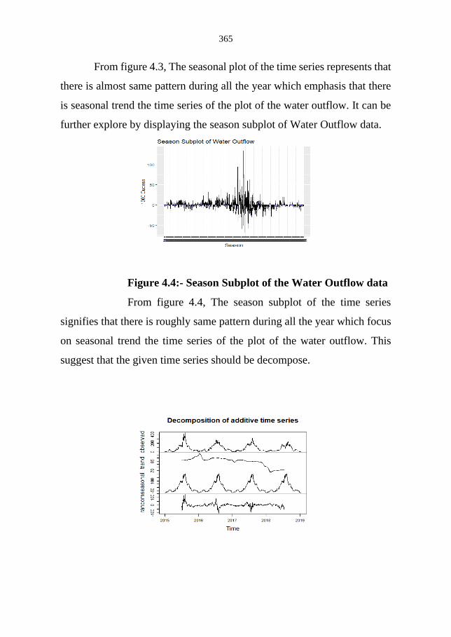
From figure 4.3, The seasonal plot of the time series represents that
there is almost same pattern during all the year which emphasis that there
is seasonal trend the time series of the plot of the water outflow. It can be
further explore by displaying the season subplot of Water Outflow data.
Figure 4.4:- Season Subplot of the Water Outflow data
From figure 4.4, The season subplot of the time series
signifies that there is roughly same pattern during all the year which focus
on seasonal trend the time series of the plot of the water outflow. This
suggest that the given time series should be decompose.

366
Figure 4.5:- Decomposition of the Water Outflow time
series
From figure 4.5, Obviously, there is seasonal trend in the
given time series of Water Outflow, it also shows that there is a
decreasing trend.
Figure 4.6:- Correlogram of the Water Outflow series
with ACF
figure 4.6, it is shown that the process is memory driven
process.
367
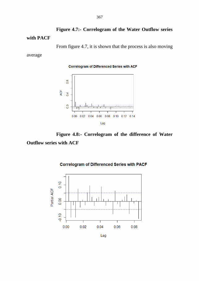
Figure 4.7:- Correlogram of the Water Outflow series
with PACF
From figure 4.7, it is shown that the process is also moving
average
Figure 4.8:- Correlogram of the difference of Water
Outflow series with ACF

368
Figure 4.9:- Correlogram of the difference of Water Outflow series
with PACF
Table 4.1 Candidate SARIMA Models
Model AIC
ARIMA(0,1,0)(0,1,0) 8828.187
ARIMA(0,1,1)(0,1,0) 8795.579
ARIMA(0,1,2)(0,1,0) 8792.474
ARIMA(0,1,3)(0,1,0) 8791.784
ARIMA(0,1,4)(0,1,0) 8756.738
ARIMA(0,1,5)(0,1,0) 8757.509
ARIMA(1,1,0)(0,1,0) 8800.982
ARIMA(1,1,1)(0,1,0) 8789.731
ARIMA(1,1,3)(0,1,0) 8774.345
ARIMA(1,1,4)(0,1,0) 8756.504
ARIMA(2,1,0)(0,1,0) 8790.907
ARIMA(2,1,1)(0,1,0) 8770.703
ARIMA(3,1,0)(0,1,0) 8787.185
ARIMA(3,1,1)(0,1,0) 8772.593
ARIMA(4,1,0)(0,1,0) 8774.229
ARIMA(4,1,1)(0,1,0) 8765.531
ARIMA(5,1,0)(0,1,0) 8773.098
In the above table the candidate models for forecasting the Water
Outflow data are tabulated, by studying the correlogram with respect to
ACF and PACF.
369
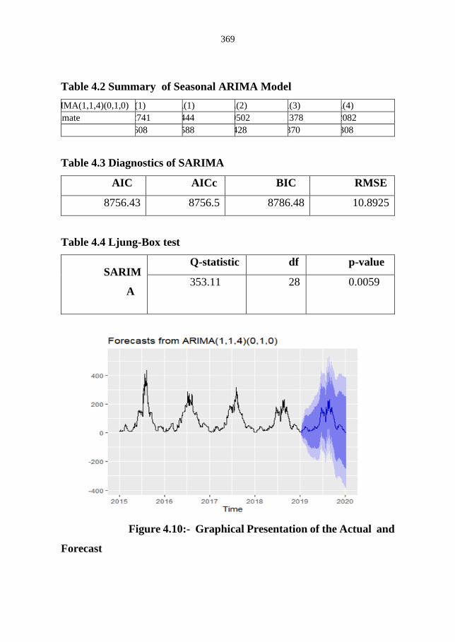
Table 4.2 Summary of Seasonal ARIMA Model
ARIMA(1,1,4)(0,1,0) AR(1) MA(1) MA(2) MA(3) MA(4)
Estimate -0.2741 0.4444 -0.0502 -0.1378 -0.2082
S.E 0.1608 0.1588 0.0428 0.0370 0.0308
Table 4.3 Diagnostics of SARIMA
AIC AICc BIC RMSE
8756.43 8756.5 8786.48 10.8925
Table 4.4 Ljung-Box test
SARIM
A
Q-statistic df p-value
353.11 28
9
0.0059
Figure 4.10:- Graphical Presentation of the Actual and
Forecast

370
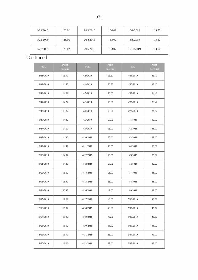
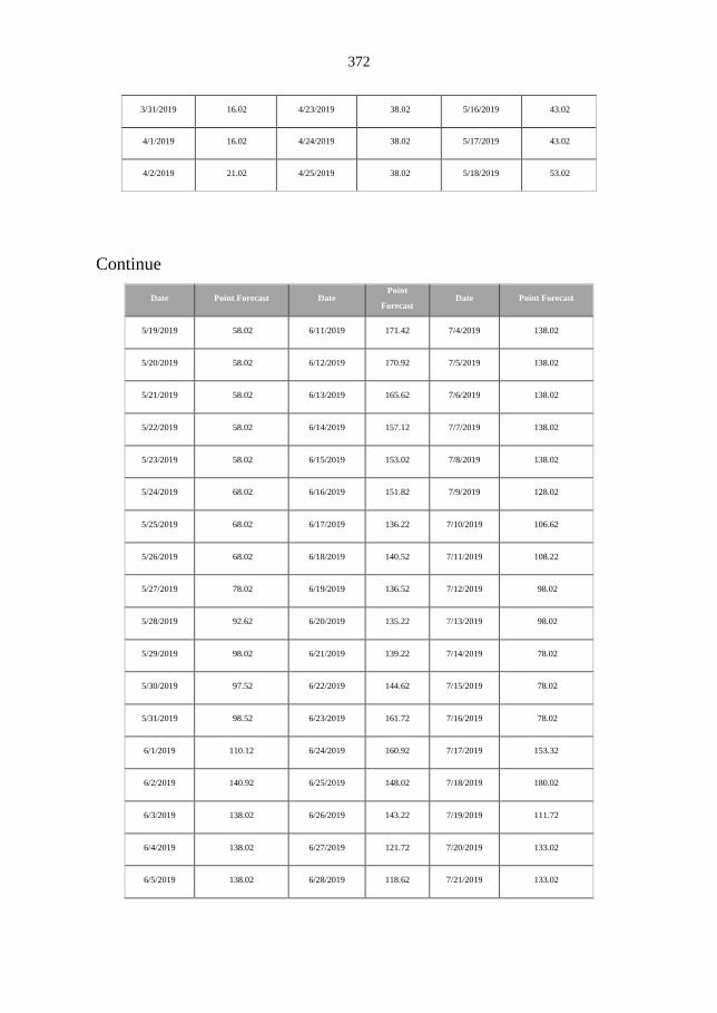
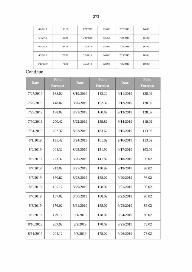
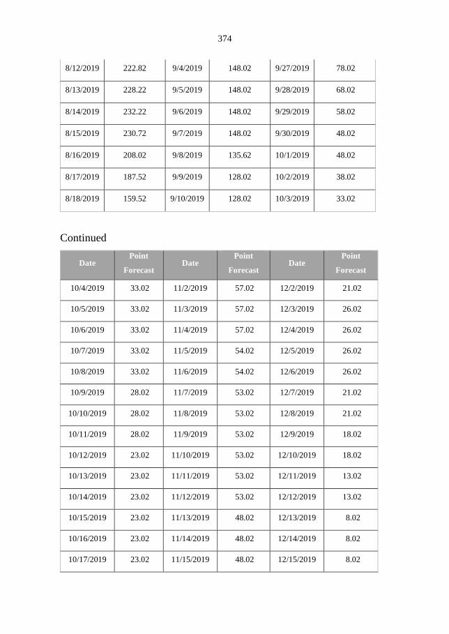
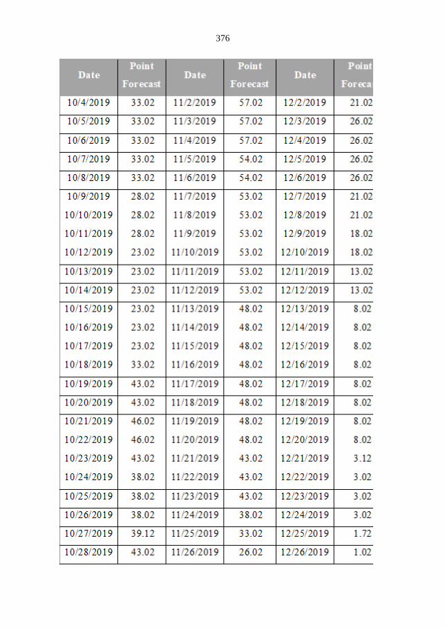
Table 4.5 Forecast Values Estimated through SARIMA Model
Date Point
Forecast Date
Point
Forecast Date
Point
Forecast
1/1/2019 2.87 1/24/2019 23.02 2/16/2019 33.02
1/2/2019 3.01 1/25/2019 30.02 2/17/2019 32.02
1/3/2019 2.98 1/26/2019 30.02 2/18/2019 29.32
1/4/2019 3.03 1/27/2019 33.02 2/19/2019 18.72
1/5/2019 15.92 1/28/2019 33.02 2/20/2019 18.72
1/6/2019 16.02 1/29/2019 40.02 2/21/2019 22.12
1/7/2019 16.02 1/30/2019 43.02 2/22/2019 17.22
1/8/2019 18.02 1/31/2019 43.02 2/23/2019 15.42
1/9/2019 20.02 2/1/2019 42.12 2/24/2019 14.22
1/10/2019 20.02 2/2/2019 38.02 2/25/2019 12.72
1/11/2019 20.02 2/3/2019 38.02 2/26/2019 12.72
1/12/2019 20.02 2/4/2019 38.02 2/27/2019 12.92
1/13/2019 20.02 2/5/2019 38.02 2/28/2019 12.32
1/14/2019 20.02 2/6/2019 38.02 3/1/2019 12.22
1/15/2019 20.02 2/7/2019 38.02 3/2/2019 11.82
1/16/2019 20.22 2/8/2019 38.02 3/3/2019 13.22
1/17/2019 19.82 2/9/2019 38.02 3/4/2019 24.42
1/18/2019 20.02 2/10/2019 38.02 3/5/2019 23.52
1/19/2019 20.02 2/11/2019 38.02 3/6/2019 18.82
1/20/2019 20.02 2/12/2019 38.02 3/7/2019 17.02
371
Continued
Date Point
Forecast Date
Point
Forecast Date
Point
Forecast
3/11/2019 15.02 4/3/2019 25.52 4/26/2019 35.72
3/12/2019 14.52 4/4/2019 30.52 4/27/2019 35.42
3/13/2019 14.22 4/5/2019 28.02 4/28/2019 34.42
3/14/2019 14.22 4/6/2019 28.02 4/29/2019 33.42
3/15/2019 13.82 4/7/2019 28.02 4/30/2019 31.52
3/16/2019 14.32 4/8/2019 28.02 5/1/2019 32.52
3/17/2019 14.12 4/9/2019 28.02 5/2/2019 38.02
3/18/2019 14.42 4/10/2019 20.02 5/3/2019 38.02
3/19/2019 14.42 4/11/2019 23.02 5/4/2019 33.02
3/20/2019 14.92 4/12/2019 23.02 5/5/2019 33.02
3/21/2019 14.82 4/13/2019 23.02 5/6/2019 32.22
3/22/2019 15.52 4/14/2019 28.02 5/7/2019 38.02
3/23/2019 18.32 4/15/2019 38.02 5/8/2019 38.02
3/24/2019 20.42 4/16/2019 43.02 5/9/2019 38.02
3/25/2019 19.02 4/17/2019 48.02 5/10/2019 43.02
3/26/2019 16.02 4/18/2019 48.02 5/11/2019 48.02
3/27/2019 16.02 4/19/2019 43.02 5/12/2019 48.02
3/28/2019 16.02 4/20/2019 38.02 5/13/2019 48.02
3/29/2019 16.02 4/21/2019 38.02 5/14/2019 43.02
3/30/2019 16.02 4/22/2019 38.02 5/15/2019 43.02
1/21/2019 23.02 2/13/2019 38.02 3/8/2019 15.72
1/22/2019 23.02 2/14/2019 33.02 3/9/2019 14.62
1/23/2019 23.02 2/15/2019 33.02 3/10/2019 13.72
372
3/31/2019 16.02 4/23/2019 38.02 5/16/2019 43.02
4/1/2019 16.02 4/24/2019 38.02 5/17/2019 43.02
4/2/2019 21.02 4/25/2019 38.02 5/18/2019 53.02
Continue
Date Point Forecast Date Point
Forecast Date Point Forecast
5/19/2019 58.02 6/11/2019 171.42 7/4/2019 138.02
5/20/2019 58.02 6/12/2019 170.92 7/5/2019 138.02
5/21/2019 58.02 6/13/2019 165.62 7/6/2019 138.02
5/22/2019 58.02 6/14/2019 157.12 7/7/2019 138.02
5/23/2019 58.02 6/15/2019 153.02 7/8/2019 138.02
5/24/2019 68.02 6/16/2019 151.82 7/9/2019 128.02
5/25/2019 68.02 6/17/2019 136.22 7/10/2019 106.62
5/26/2019 68.02 6/18/2019 140.52 7/11/2019 108.22
5/27/2019 78.02 6/19/2019 136.52 7/12/2019 98.02
5/28/2019 92.62 6/20/2019 135.22 7/13/2019 98.02
5/29/2019 98.02 6/21/2019 139.22 7/14/2019 78.02
5/30/2019 97.52 6/22/2019 144.62 7/15/2019 78.02
5/31/2019 98.52 6/23/2019 161.72 7/16/2019 78.02
6/1/2019 110.12 6/24/2019 160.92 7/17/2019 153.32
6/2/2019 140.92 6/25/2019 148.02 7/18/2019 180.02
6/3/2019 138.02 6/26/2019 143.22 7/19/2019 111.72
6/4/2019 138.02 6/27/2019 121.72 7/20/2019 133.02
6/5/2019 138.02 6/28/2019 118.62 7/21/2019 133.02
373
6/6/2019 136.12 6/29/2019 120.82 7/22/2019 148.02
6/7/2019 139.92 6/30/2019 136.52 7/23/2019 153.02
6/8/2019 167.12 7/1/2019 148.02 7/24/2019 163.02
6/9/2019 178.02 7/2/2019 148.02 7/25/2019 163.02
6/10/2019 178.02 7/3/2019 138.02 7/26/2019 168.02
Continue
Date Point
Forecast Date
Point
Forecast Date
Point
Forecast
7/27/2019 168.02 8/19/2019 143.22 9/11/2019 128.02
7/28/2019 148.02 8/20/2019 152.32 9/12/2019 128.02
7/29/2019 138.02 8/21/2019 160.82 9/13/2019 128.02
7/30/2019 200.42 8/22/2019 159.82 9/14/2019 118.02
7/31/2019 202.32 8/23/2019 163.62 9/15/2019 113.02
8/1/2019 195.42 8/24/2019 161.82 9/16/2019 113.02
8/2/2019 204.32 8/25/2019 151.92 9/17/2019 103.02
8/3/2019 223.32 8/26/2019 141.82 9/18/2019 98.02
8/4/2019 212.02 8/27/2019 130.92 9/19/2019 98.02
8/5/2019 180.62 8/28/2019 158.02 9/20/2019 98.02
8/6/2019 155.12 8/29/2019 158.02 9/21/2019 98.02
8/7/2019 157.02 8/30/2019 168.02 9/22/2019 98.02
8/8/2019 176.02 8/31/2019 168.02 9/23/2019 83.02
8/9/2019 179.12 9/1/2019 178.02 9/24/2019 83.02
8/10/2019 207.92 9/2/2019 178.02 9/25/2019 78.02
8/11/2019 204.12 9/3/2019 178.02 9/26/2019 78.02
374
8/12/2019 222.82 9/4/2019 148.02 9/27/2019 78.02
8/13/2019 228.22 9/5/2019 148.02 9/28/2019 68.02
8/14/2019 232.22 9/6/2019 148.02 9/29/2019 58.02
8/15/2019 230.72 9/7/2019 148.02 9/30/2019 48.02
8/16/2019 208.02 9/8/2019 135.62 10/1/2019 48.02
8/17/2019 187.52 9/9/2019 128.02 10/2/2019 38.02
8/18/2019 159.52 9/10/2019 128.02 10/3/2019 33.02
Continued
Date Point
Forecast Date
Point
Forecast Date
Point
Forecast
10/4/2019 33.02 11/2/2019 57.02 12/2/2019 21.02
10/5/2019 33.02 11/3/2019 57.02 12/3/2019 26.02
10/6/2019 33.02 11/4/2019 57.02 12/4/2019 26.02
10/7/2019 33.02 11/5/2019 54.02 12/5/2019 26.02
10/8/2019 33.02 11/6/2019 54.02 12/6/2019 26.02
10/9/2019 28.02 11/7/2019 53.02 12/7/2019 21.02
10/10/2019 28.02 11/8/2019 53.02 12/8/2019 21.02
10/11/2019 28.02 11/9/2019 53.02 12/9/2019 18.02
10/12/2019 23.02 11/10/2019 53.02 12/10/2019 18.02
10/13/2019 23.02 11/11/2019 53.02 12/11/2019 13.02
10/14/2019 23.02 11/12/2019 53.02 12/12/2019 13.02
10/15/2019 23.02 11/13/2019 48.02 12/13/2019 8.02
10/16/2019 23.02 11/14/2019 48.02 12/14/2019 8.02
10/17/2019 23.02 11/15/2019 48.02 12/15/2019 8.02

375
10/18/2019 33.02 11/16/2019 48.02 12/16/2019 8.02
10/19/2019 43.02 11/17/2019 48.02 12/17/2019 8.02
10/20/2019 43.02 11/18/2019 48.02 12/18/2019 8.02
10/21/2019 46.02 11/19/2019 48.02 12/19/2019 8.02
10/22/2019 46.02 11/20/2019 48.02 12/20/2019 8.02
10/23/2019 43.02 11/21/2019 43.02 12/21/2019 3.12
10/24/2019 38.02 11/22/2019 43.02 12/22/2019 3.02
10/25/2019 38.02 11/23/2019 43.02 12/23/2019 3.02
10/26/2019 38.02 11/24/2019 38.02 12/24/2019 3.02
10/27/2019 39.12 11/25/2019 33.02 12/25/2019 1.72
10/28/2019 43.02 11/26/2019 26.02 12/26/2019 1.02
10/29/2019 53.02 11/27/2019 26.02 12/27/2019 0.52
10/30/2019 57.02 11/28/2019 26.02 12/28/2019 1.02
10/31/2019 57.02 11/29/2019 24.92 12/29/2019 1.02
11/1/2019 57.02 11/30/2019 23.02 12/30/2019 1.02
10/27/2019 39.12 12/1/2019 23.02 12/31/2019 1.02
376
377
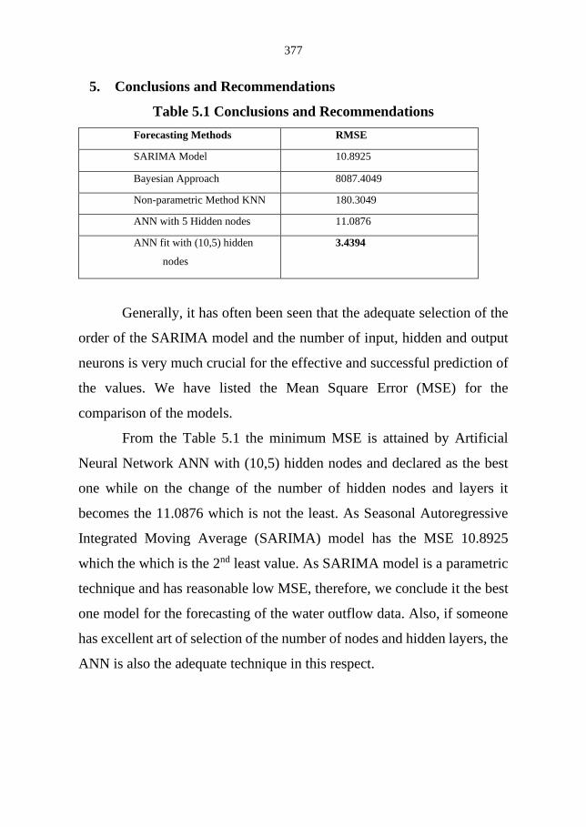
5. Conclusions and Recommendations
Table 5.1 Conclusions and Recommendations
Forecasting Methods RMSE
SARIMA Model 10.8925
Bayesian Approach 8087.4049
Non-parametric Method KNN 180.3049
ANN with 5 Hidden nodes 11.0876
ANN fit with (10,5) hidden
nodes
3.4394
Generally, it has often been seen that the adequate selection of the
order of the SARIMA model and the number of input, hidden and output
neurons is very much crucial for the effective and successful prediction of
the values. We have listed the Mean Square Error (MSE) for the
comparison of the models.
From the Table 5.1 the minimum MSE is attained by Artificial
Neural Network ANN with (10,5) hidden nodes and declared as the best
one while on the change of the number of hidden nodes and layers it
becomes the 11.0876 which is not the least. As Seasonal Autoregressive
Integrated Moving Average (SARIMA) model has the MSE 10.8925
which the which is the 2nd least value. As SARIMA model is a parametric
technique and has reasonable low MSE, therefore, we conclude it the best
one model for the forecasting of the water outflow data. Also, if someone
has excellent art of selection of the number of nodes and hidden layers, the
ANN is also the adequate technique in this respect.
378
6. References
Adhikari K., R., & R.K., A. (2013). An Introductory Study on Time Series
Modeling and Forecasting Ratnadip Adhikari R. K. Agrawal. ArXiv
Preprint ArXiv:1302.6613. https://doi.org/10.1210/jc.2006-1327
Cai, H., Lye, L. M., & Khan, A. (2009). Flood forecasting on the Humber
river using an artificial neural network approach (Vol. 2).
Chatfield, C. (1996). Model Uncertainty and Forecast Accuracy. Journal
of Forecasting, 15(July), 495–508.
Elganainy, M. A., & Eldwer, A. E. (2018). Stochastic Forecasting Models
of the Monthly Streamflow for the Blue Nile at Eldiem Station 1.
45(3), 326–327. https://doi.org/10.1134/S0097807818030041
Hipel, K. W. (1994). TIME SERIES MODELLING OF WATER
RESOURCES AND ENVIRONMENTAL SYSTEMS. 1994.
Jam, F. A. (2013). Time Series Model to Forecast Area of Mangoes from
Pakistan : An Application of Univariate Arima Model. (December
2012), 10–15.
Jones, A. L., & Smart, P. L. (2005). Spatial and temporal changes in the
structure of groundwater nitrate concentration time series (1935-
1999) as demonstrated by autoregressive modelling. Journal of
Hydrology, 310(1–4), 201–215.
https://doi.org/10.1016/j.jhydrol.2005.01.002
Klose, C., Pircher, M., & Sharma, S. (2004). Univariate time series
Forecasting. (9706253).
Merkuryeva, G. V., & Kornevs, M. (2014). Water Flow Forecasting and
River Simulation for Flood Risk Analysis. Information Technology
and Management Science, 16(1). https://doi.org/10.2478/itms-2013-
0006

379
Mills, T. C. (2015). Time Series Econometrics: A Concise Introduction.
https://doi.org/10.1016/S1062-9769(96)90007-1
Naveena, K., Singh, S., Rathod, S., & Singh, A. (2017). Hybrid ARIMA-
ANN Modelling for Forecasting the Price of Robusta Coffee in
Hybrid ARIMA-ANN Modelling for Forecasting the Price of Robusta
Coffee in India. International Journal of Current Microbiology and
Applied Sciences, 6(7), 1721–1726.
https://doi.org/10.20546/ijcmas.2017.607.207
Rbunaru, A. B. Ă. C. Ă., & Cescu, L. M. C. Ă. (2013). Methods Used in
the Seasonal Variations Analysis Of Time Series. Revista Română de
Statistică, 61(3), 12–18.
Sarjinder Singh. (2003). Advanced Sampling Theory with Applications.
https://doi.org/10.1017/CBO9781107415324.004
Seymour, L., Brockwell, P. J., & Davis, R. A. (1997). Introduction to Time
Series and Forecasting. In Journal of the American Statistical
Association (Vol. 92). https://doi.org/10.2307/2965440
Since, I., & Model, J. (2008). Improving artificial neural networks ’
performance in seasonal time series forecasting. Information
Sciences, 178, 4550–4559. https://doi.org/10.1016/j.ins.2008.07.024
Valipour, M., Banihabib, M. E., Mahmood, S., & Behbahani, R. (2013).
Comparison of the ARMA , ARIMA , and the autoregressive artificial
neural network models in forecasting the monthly inflow of Dez dam
reservoir. Journal of Hydrology, 476, 433–441.
https://doi.org/10.1016/j.jhydrol.2012.11.017