1

35th International North Sea Flow Measurement Workshop 2017

Fiscal Metering Systems Mismeasurement Management Experiences in Petronas

Wan Adrie Wan Ahmad, PETRONAS, Malaysia

Han van Dal, ABB, The Netherlands

1 INTRODUCTION

Mismeasurement management is about the detection and correction of systematic

measurement errors in hydrocarbon quantities reported by a custody transfer flow

metering system. A systematic (deterministic) error is due to an assignable cause, such as

a transmitter failure, a disturbed meter pulse signal, a faulty parameter value or a

measurement that fails its validation. This opposed to a non-deterministic error which is

caused by natural variance.

The correction of a measurement error is not an obvious task and requires in-depth

analysis of all available information to determine an accurate substitution for the faulty

value. A poor correction could increase the error instead of rectifying it. A separate

correction is required for every associated transaction, e g. a transmitter failing its

quarterly validation may require the correction of dozens of daily reports.

Since 2014 Petronas has been automating the correction of measurement errors in a few

its largest flow metering systems. This paper describes the error correction methodology

[1] used in and field experiences with these systems.

2 MISMEASUREMENT DETECTION

Most metering control systems use the alarms that are generated by the flow computers

to detect measurement problems but do not provide more sophisticated functionality to

2

detect less obvious measurement errors. For this reason the Petronas flow metering

systems use a number of additional detection methods.

2.1 Data validity checks

A simple yet highly effective check is to verify that a live measurement is continuously

updated. An input value can be considered as ‘frozen’ and therefore invalid when its value

does not change for a specific time period, e.g. 30 seconds.

Most flow computers apply limit and sometimes also rate of change checks on the field

inputs such as temperature, pressure and density. The actual low and high limit values are

usually set by operations and do not necessarily reflect measurement integrity. Therefore

a second set of limit checks is applied that are not controlled by operations but by the

metering engineers instead. Limits checks are also applied on the main gas components

2.2 Discrepancy checks

Redundant measurements provide the capability to automatically check for discrepancies.

Examples of such redundant measurements are:

• Multiple dP transmitters measuring the same differential pressure.

• Dual station densitometers or gas chromatographs installed at the header.

• A density measured by a densitometer and inferred from a gas composition.

• A standard density determined in the laboratory and the corresponding value

calculated by a flow computer.

• A pressure, temperature or density measurement on a prover compared to values

of the lined up meter run

• A PRT element in a densitometer or flow meter and the primary temperature

transmitter

• Process flow meters that are compared with the custody transfer meters

• Speed of sound measured by an ultrasonic flow meter and calculated from the

fluid composition.

• A flow metering system with two or more flowing meter runs (parallel run data).

2.3 Logical checks

The correct operation of the measurement system is verified by applying a number of

basic checks.

• A flow computer should not register flow while the meter run is closed unless

maintenance is applied to the flow computer.

3

• An open meter run should indicate flow when parallel runs that are part of the

same metering skid are registering flow.

• A flow meter shall not operate outside its calibrated range for a longer period of

time. Most flow meters are calibrated in specific part of the full flow range,

typically between 20% and 95%. Operating the meter outside this range may

cause a systematic error.

• For a differential pressure (dP) type of flow meter with multiple dP transmitters

operating in different dP ranges, the flow computer must use the correct dP

transmitter for its flow calculations

• The real-time clock used by the flow computers should not deviate significantly

from an external reference clock. This is especially of interest to continuous

production systems in which quantities are reported on a periodic, typically hourly

or daily, basis.

3 SUBSTITUTION VALUES

A different type of substitution value is required for a mismeasurement caused by a

measurement failure than for a mismeasurement caused by a measurement offset (shift or

drift)..

When a validation of an instrument fails, it is typically recalibrated and then validated

again. The offset between the as-found and as-left validation is an indication for the

adjustment of the instrument and the substitution value used for the error corrections will

be the original measurement compensated for the adjustment.

When the original measurement value is faulty, then the substitution value has to be

determined in another way. As explained further down this paper an accurate substitution

value requires some sort of redundant measurement information.

• Redundant sensor

Obviously the most accurate substitution value is provided by a redundant

instrument, for example a dual gas chromatograph or a dual temperature

transmitter.

• Secondary measurement

Any other direct or inferred measurement of the same property, for example a

pressure measurement on a gas compressor, a flow meter used for process control,

a density calculated from compositional data or a transmitter installed at the

header or the prover.

4

• Parallel meter run data

For a flow metering system with two or more parallel meter runs the substitution

value can be derived from the measurement data of the other meter run(s) that was

/were flowing at the time of the failure.

When no redundant information is available for the error correction, there is no other

option than to use data from before and after the failure. Several averaging methods are

used in this case such as:

• Period Average

The average value of a particular period (e.g. 7 days) before and after the

mismeasurement

• Moving Average

The moving average over a configurable period (e.g. 1 hour) just before the issue

occurred.

• Linear interpolation

The average of the instantaneous values just before and after the failure

• Last good value

The instantaneous value just before the issue occurred is used as the corrected

value.

4 RECALCULATIONS

The Petronas flow metering systems are able to automatically quantify a measurement

error allowing the user to quickly assess the impact of a mismeasurement issue.

4.1 Recalculation methodology

The recalculation methodology is in accordance with API MPMS 21.1 [2], which sets the

requirements for online and offline computations to determine accurate flow quantities.

The standard specifies two different methods to compute the flow rate from the sampled

input data.

1. A Full Flow Rate Calculation is performed (at least) once per second based on the

sampled input data. This is the method used by all the current flow computers.

5

2. If the full flow rate calculation can’t be performed every second, then the method

called Factored Flow Rate Calculation can be used instead. This method involves

1 second sampling of the inputs and a less frequent (typically once every 5

minutes) flow calculation based on averaged input data. Although less accurate

than the first method, this method provides custody transfer grade of accuracy as

well.

For recalculations it is not practical to perform a full flow calculation, because this would

require the storage and processing of data with 1 second resolution. Therefore the

'Factored Flow rate Calculation' method is used to average and archive data that can later

be used for the error corrections.

For the Factored Flow Rate Calculation Method the flow equation is factored in two parts.

One part contains the live inputs that may change considerably with time, while the other

part contains the live inputs that remain relatively constant with respect to time.

𝑄𝑖 = 𝐼𝑀𝑉𝑥𝐷𝑉𝑖

Where:

Qi flow rate based on data taken at sample i

IMV Integral Multiplier Value, representing the static variables

DVi Dynamic Variables, representing the live inputs, taken at sample i

For the Factored Flow Rate Calculation the flow quantity is calculated over a number of

samples.

𝑄 = 𝐼𝑀𝑉 ∑ 𝐷𝑉𝑖

𝑖=𝑛

𝑖=1

∆𝑡𝑖

Where:

Q flow quantity over n sample

Δti sampling interval

The term ∑ 𝐷𝑉𝑖𝑖=𝑛𝑖=1 ∆𝑡𝑖 is called the Integral Value (IV), such that:

𝑄 = 𝐼𝑀𝑉𝑥𝐼𝑉

6

IMV is calculated at the end of each integration period using the flow dependent linear

averages of the dynamic variables at the end of the period,

4.2 Quantity Calculation Period (QCP)

The integration period used for the determination of the IV is called the Quantity

Calculation Period (QCP).

𝑄𝐶𝑃 = ∑ ∆𝑡𝑖

𝑖=𝑛

𝑖=1

The standard states that the QCP should not exceed 5 minutes. Longer periods may be

used if it can be demonstrated that the additional uncertainty is no more than 0.05%.

However, because the methodology is used for a large number of installations with very

different flow regimes and process conditions, it is unknown if the actual additional

accuracy will exceed the 0.05% limit. Therefore the methodology uses Quantity

Calculation Periods of 5 minutes each.

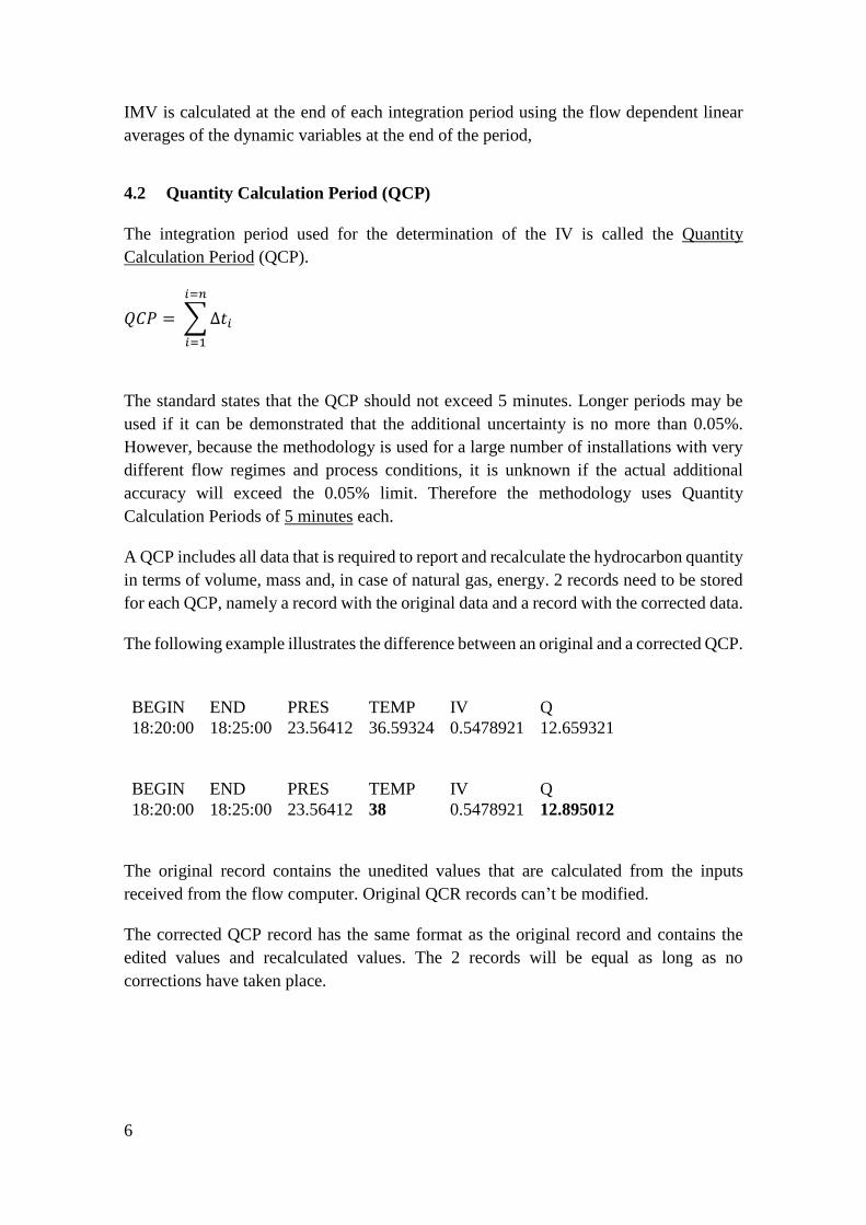
A QCP includes all data that is required to report and recalculate the hydrocarbon quantity

in terms of volume, mass and, in case of natural gas, energy. 2 records need to be stored

for each QCP, namely a record with the original data and a record with the corrected data.

The following example illustrates the difference between an original and a corrected QCP.

BEGIN END PRES TEMP IV Q

18:20:00 18:25:00 23.56412 36.59324 0.5478921 12.659321

BEGIN END PRES TEMP IV Q

18:20:00 18:25:00 23.56412 38 0.5478921 12.895012

The original record contains the unedited values that are calculated from the inputs

received from the flow computer. Original QCR records can’t be modified.

The corrected QCP record has the same format as the original record and contains the

edited values and recalculated values. The 2 records will be equal as long as no

corrections have taken place.

7

4.3 Integral Value for differential meters

The standard makes a distinction between differential and linear flow meters. Differential

flow meters like an orifice and a venturi flow meter, measure the differential pressure

drop over the primary flow element. Because the relation between the differential pressure

and the flow is non-linear the averaging and recalculation methodology is different from

linear flow meters (e.g. turbine and ultrasonic flow meters).

For differential flow meters the dynamic variables are differential pressure, static pressure

and temperature. These variables need therefore be sampled at least once per second and

a corresponding flow dependent linear average needs to be determined for each QCP.

API MPMS 21.1 states that at a minimum the Integral Value for differential flow meters

will include the differential pressure and the static pressure, assuming that these two

variables may show a relative large fluctuation in comparison to other inputs including

temperature.

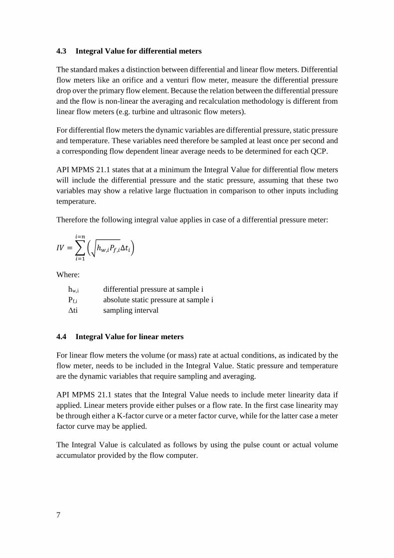
Therefore the following integral value applies in case of a differential pressure meter:

𝐼𝑉 = ∑ (√ℎ𝑤,𝑖𝑃𝑓,𝑖∆𝑡𝑖)

𝑖=𝑛

𝑖=1

Where:

hw,i differential pressure at sample i

Pf,i absolute static pressure at sample i

Δti sampling interval

4.4 Integral Value for linear meters

For linear flow meters the volume (or mass) rate at actual conditions, as indicated by the

flow meter, needs to be included in the Integral Value. Static pressure and temperature

are the dynamic variables that require sampling and averaging.

API MPMS 21.1 states that the Integral Value needs to include meter linearity data if

applied. Linear meters provide either pulses or a flow rate. In the first case linearity may

be through either a K-factor curve or a meter factor curve, while for the latter case a meter

factor curve may be applied.

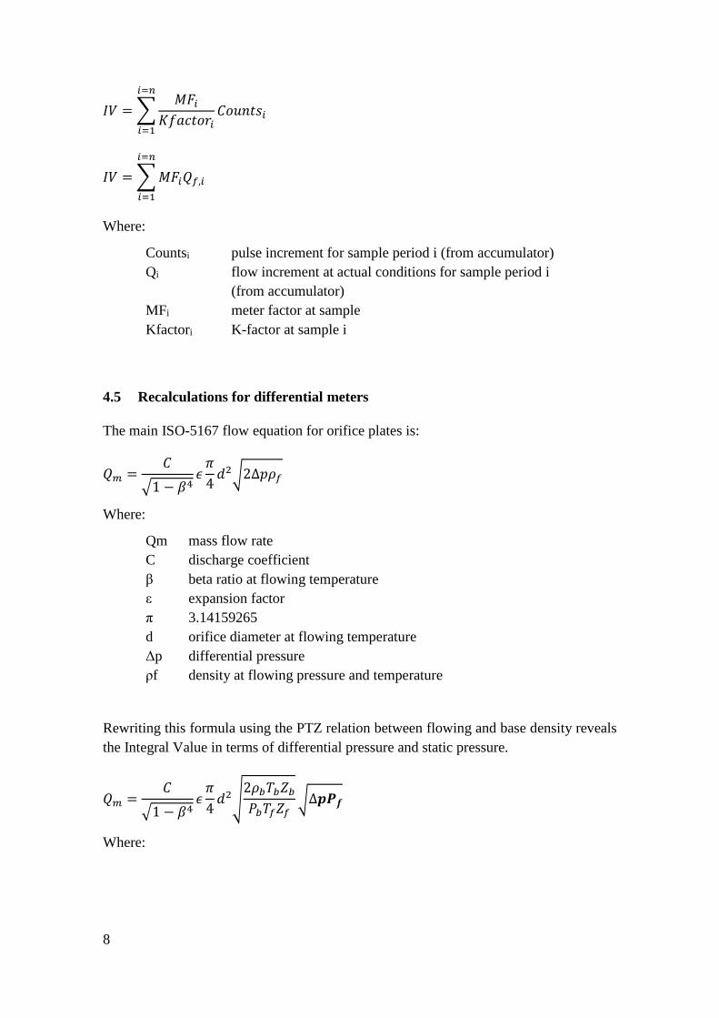
The Integral Value is calculated as follows by using the pulse count or actual volume

accumulator provided by the flow computer.

8

𝐼𝑉 = ∑𝑀𝐹𝑖

𝐾𝑓𝑎𝑐𝑡𝑜𝑟𝑖𝐶𝑜𝑢𝑛𝑡𝑠𝑖

𝑖=𝑛

𝑖=1

𝐼𝑉 = ∑ 𝑀𝐹𝑖𝑄𝑓,𝑖

𝑖=𝑛

𝑖=1

Where:

Countsi pulse increment for sample period i (from accumulator)

Qi flow increment at actual conditions for sample period i

(from accumulator)

MFi meter factor at sample

Kfactori K-factor at sample i

4.5 Recalculations for differential meters

The main ISO-5167 flow equation for orifice plates is:

𝑄𝑚 =𝐶

√1 − 𝛽4𝜖

𝜋

4𝑑2√2∆𝑝𝜌𝑓

Where:

Qm mass flow rate

C discharge coefficient

β beta ratio at flowing temperature

ε expansion factor

π 3.14159265

d orifice diameter at flowing temperature

Δp differential pressure

ρf density at flowing pressure and temperature

Rewriting this formula using the PTZ relation between flowing and base density reveals

the Integral Value in terms of differential pressure and static pressure.

𝑄𝑚 =𝐶

√1 − 𝛽4𝜖

𝜋

4𝑑2√

2𝜌𝑏𝑇𝑏𝑍𝑏

𝑃𝑏𝑇𝑓𝑍𝑓√∆𝒑𝑷𝒇

Where:

9

Pf flowing static pressure absolute

Tf flowing temperature

Zf compressibility at flowing pressure and temperature

ρb density at base pressure and temperature

Pb base static pressure absolute

Tb base temperature

Zb compressibility at base pressure and temperature

Recalculations are based on QCP records. For each QCP the Integral Value √∆𝑝𝑃𝑓 has

been calculated and stored together with the flow-dependent linear averages of the

differential pressure, flowing static pressure and flowing temperature. Also the Flowing

time (FT) is stored for each QCP record, which is the time within the QCP that the flow

was above the No Flow Cut-off Limit. The remaining variables used in the flow equation

are either stored as a constant value to the QCP record or recalculated from the flow-

dependent linear averages of the dynamic variables and in case of the compressibility and

density, the gas composition. Therefore each QCP record also holds the values for the

individual gas components that were determined at the latest chromatograph cycle.

4.6 Recalculations for linear meters

The main flow equation for linear meters is:

𝑄𝑏 = (𝑃𝑓

𝑃𝑏) (

𝑇𝑏

𝑇𝑓) (

𝑍𝑏

𝑍𝑓) 𝐼𝑉

Where:

Qb base volume flow rate

Pf flowing static pressure absolute

Tf flowing temperature

Zf compressibility at flowing pressure and temperature

Pb reference static pressure absolute

Tb base temperature

Zb compressibility at base pressure and temperature

IV Integral Value

Each QCP record contains the Integral Value, the flow-dependent linear averages of

flowing static pressure and flowing temperature, the Flowing time and the gas

composition. The reference pressure and temperature are stored in the QCP record, while

the compressibility values are calculated.

10

4.7 Quantity Transaction Record (QTR)

API MPMS Chapter 21 applies the term Quantity Transaction Record (QTR) for an

hourly or daily report or a measurement ticket.

The standard requires that a whole number of QCPs fits in one QTR. The underlying

reason is that the recalculation of a QTR is most accurate when the corresponding QCPs

represent exactly the same period of time. For this purpose a QCP is ended at hourly

rollovers as well as batch ends.

Two types of QTRs are stored. The original QTR contains the unedited custody transfer

data as received from the flow computer and can’t be changed by the user, while the

corrected QTR contains the corrected data.

The hydrocarbon quantities of a corrected QTR are calculated as follows:

𝐶𝑜𝑟𝑟𝑒𝑐𝑡𝑒𝑑 𝑄𝑇𝑅 = ∑ 𝑄 𝑓𝑟𝑜𝑚 𝑐𝑜𝑟𝑟𝑒𝑐𝑡𝑒𝑑 𝑄𝐶𝑃

∑ 𝑄 𝑓𝑟𝑜𝑚 𝑜𝑟𝑖𝑔𝑖𝑛𝑎𝑙 𝑄𝐶𝑃×𝑂𝑟𝑖𝑔𝑖𝑛𝑎𝑙 𝑄𝑇𝑅

5 BASIC MISMEASUREMENT EXAMPLE

Consider an example where a flow rate is calculated from two inputs x and y (flow rate =

x * y) and suppose that input x fails for 22 minutes within a single hour and that during

the failure the last good value remains in use for the flow rate calculation.

The result is that the reported hourly total differs by 18 percent from the actual value that

would have been calculated when no failure would have occurred.

Figure 1: Basic recalculation example

11

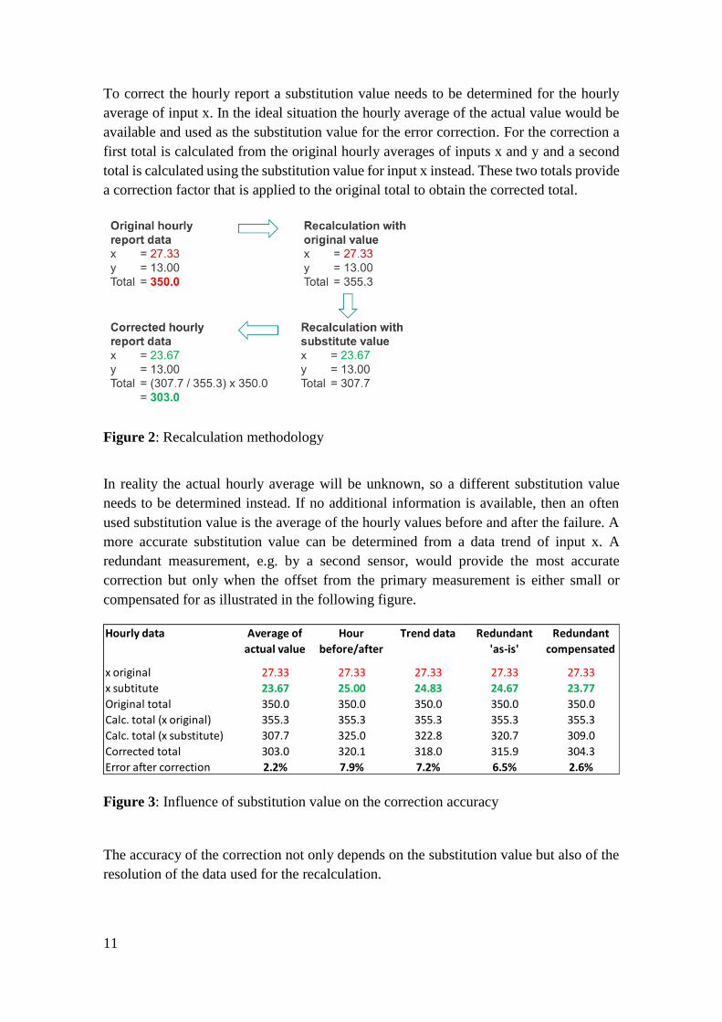
To correct the hourly report a substitution value needs to be determined for the hourly

average of input x. In the ideal situation the hourly average of the actual value would be

available and used as the substitution value for the error correction. For the correction a

first total is calculated from the original hourly averages of inputs x and y and a second

total is calculated using the substitution value for input x instead. These two totals provide

a correction factor that is applied to the original total to obtain the corrected total.

Figure 2: Recalculation methodology

In reality the actual hourly average will be unknown, so a different substitution value

needs to be determined instead. If no additional information is available, then an often

used substitution value is the average of the hourly values before and after the failure. A

more accurate substitution value can be determined from a data trend of input x. A

redundant measurement, e.g. by a second sensor, would provide the most accurate

correction but only when the offset from the primary measurement is either small or

compensated for as illustrated in the following figure.

Figure 3: Influence of substitution value on the correction accuracy

The accuracy of the correction not only depends on the substitution value but also of the

resolution of the data used for the recalculation.

Hourly data Average of

actual value

Hour

before/after

Trend data Redundant

'as-is'

Redundant

compensated

x original 27.33 27.33 27.33 27.33 27.33

x subtitute 23.67 25.00 24.83 24.67 23.77

Original total 350.0 350.0 350.0 350.0 350.0

Calc. total (x original) 355.3 355.3 355.3 355.3 355.3

Calc. total (x substitute) 307.7 325.0 322.8 320.7 309.0

Corrected total 303.0 320.1 318.0 315.9 304.3

Error after correction 2.2% 7.9% 7.2% 6.5% 2.6%

12

For instance, averaging and logging the inputs at a 5 minutes interval in accordance with

the methodology described in this paper, would significantly improve the correction of

the hourly total.

Figure 4: Influence of data resolution on correction accuracy

From the basic example it can be concluded that the accuracy of the error correction is

determined by the accuracy of the substitution value and the resolution of the

measurement data.

6 FIELD EXPERIENCES

The following cases describe actual mismeasurements that have occurred in a gas flow

metering system with 4 parallel meter runs of which 3 meter runs are flowing and 1 run

is closed. Each meter run has both a panel-mount flow computer and a field-mount flow

computer, both with their own set of dP transmitters, pressure and temperature

transmitters. Because this system has both redundant measuring instruments for each

meter run and multiple flowing runs, it provides two type of substitution values, creating

an ideal environment for field-testing the mismeasurement management functionality.

6.1 Practical case: Transmitter failure

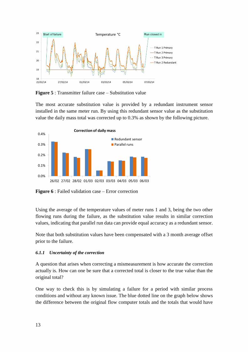
In February 2014 the primary temperature transmitter of meter run 2 failed, causing the

flow computer to fall back to a value of 19 degrees Celsius.

9 days after the failure occurred run 4 was opened and run 2 was closed. The following

graph shows the primary temperature value recorded during the failure period for meter

runs 1 and 3 and by the redundant value of run 2. The daily fluctuations are due to the

ambient temperature and solar radiation.

Error after correction Average of

actual value

Trend data Redundant

'as-is'

Redundant

compensated

Hourly data 2.2% 7.2% 6.5% 2.6%

5 minutely data 0.1% 6.6% 2.7% 0.4%

13

Figure 5 : Transmitter failure case – Substitution value

The most accurate substitution value is provided by a redundant instrument sensor

installed in the same meter run. By using this redundant sensor value as the substitution

value the daily mass total was corrected up to 0.3% as shown by the following picture.

Figure 6 : Failed validation case – Error correction

Using the average of the temperature values of meter runs 1 and 3, being the two other

flowing runs during the failure, as the substitution value results in similar correction

values, indicating that parallel run data can provide equal accuracy as a redundant sensor.

Note that both substitution values have been compensated with a 3 month average offset

prior to the failure.

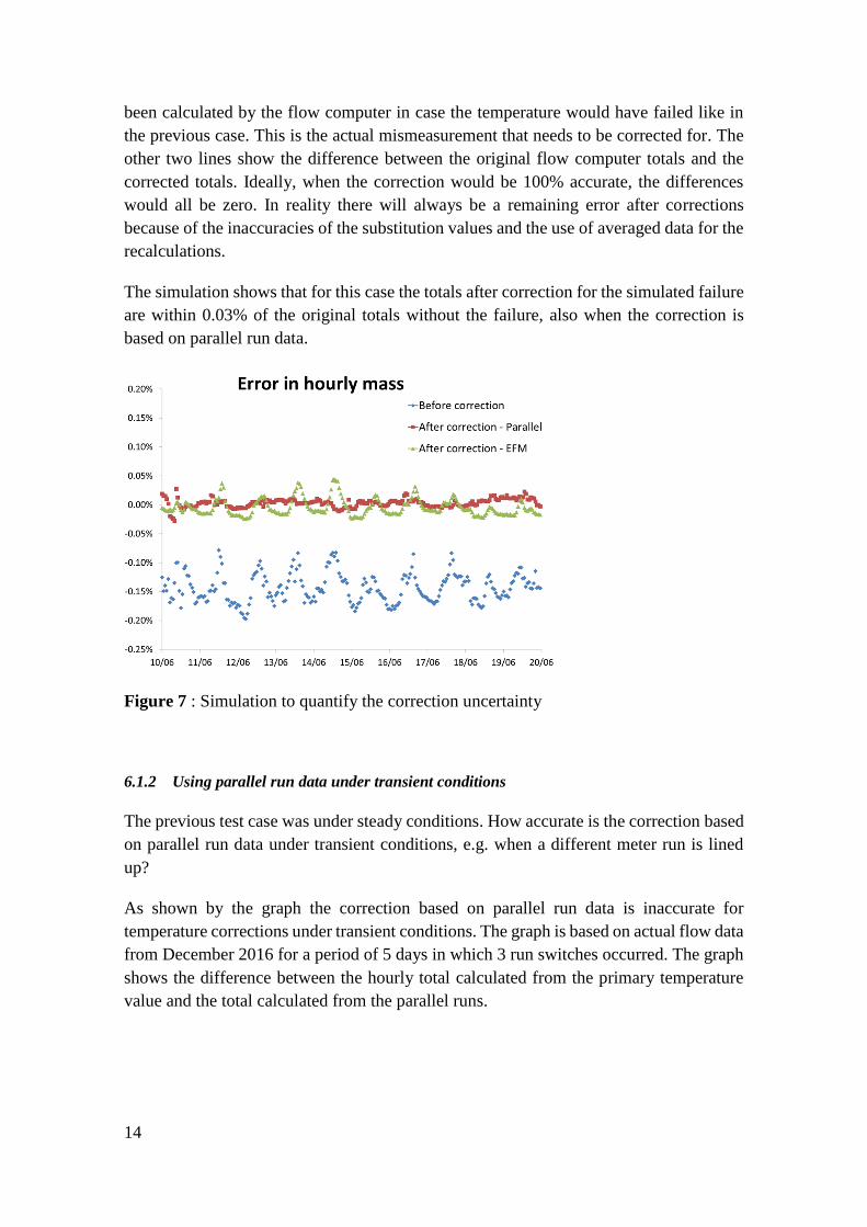
6.1.1 Uncertainty of the correction

A question that arises when correcting a mismeasurement is how accurate the correction

actually is. How can one be sure that a corrected total is closer to the true value than the

original total?

One way to check this is by simulating a failure for a period with similar process

conditions and without any known issue. The blue dotted line on the graph below shows

the difference between the original flow computer totals and the totals that would have

14

been calculated by the flow computer in case the temperature would have failed like in

the previous case. This is the actual mismeasurement that needs to be corrected for. The

other two lines show the difference between the original flow computer totals and the

corrected totals. Ideally, when the correction would be 100% accurate, the differences

would all be zero. In reality there will always be a remaining error after corrections

because of the inaccuracies of the substitution values and the use of averaged data for the

recalculations.

The simulation shows that for this case the totals after correction for the simulated failure

are within 0.03% of the original totals without the failure, also when the correction is

based on parallel run data.

Figure 7 : Simulation to quantify the correction uncertainty

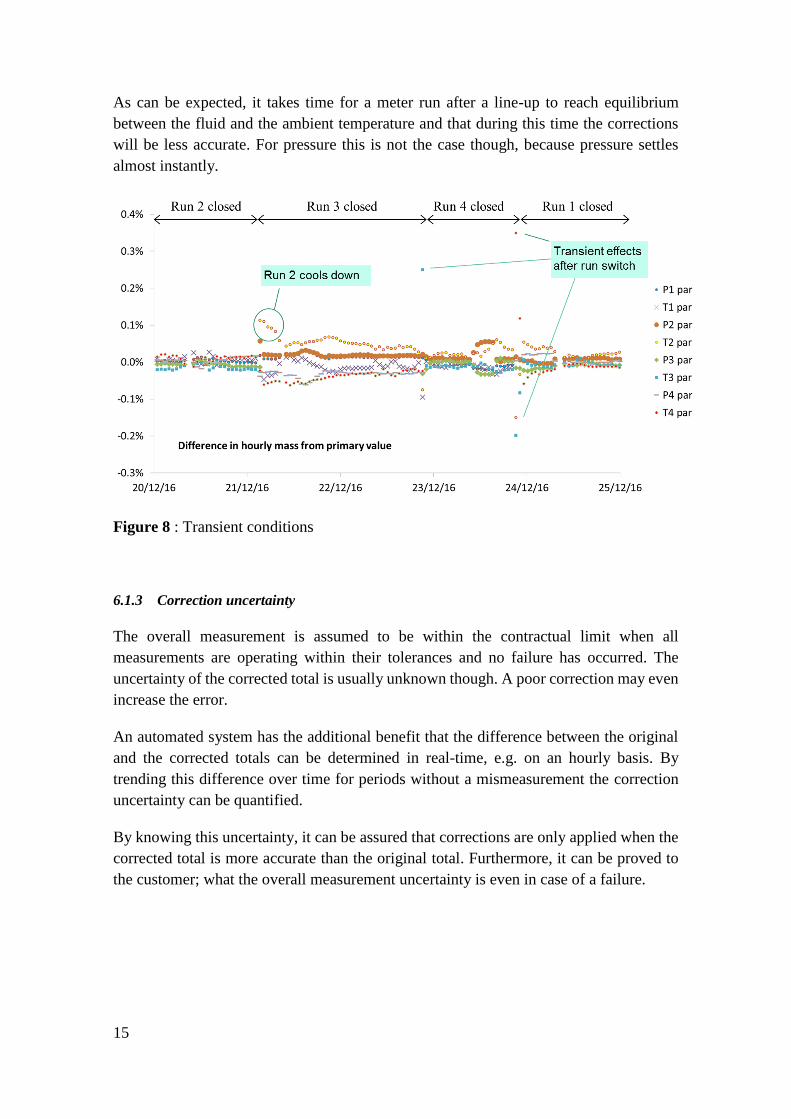
6.1.2 Using parallel run data under transient conditions

The previous test case was under steady conditions. How accurate is the correction based

on parallel run data under transient conditions, e.g. when a different meter run is lined

up?

As shown by the graph the correction based on parallel run data is inaccurate for

temperature corrections under transient conditions. The graph is based on actual flow data

from December 2016 for a period of 5 days in which 3 run switches occurred. The graph

shows the difference between the hourly total calculated from the primary temperature

value and the total calculated from the parallel runs.

15

As can be expected, it takes time for a meter run after a line-up to reach equilibrium

between the fluid and the ambient temperature and that during this time the corrections

will be less accurate. For pressure this is not the case though, because pressure settles

almost instantly.

Figure 8 : Transient conditions

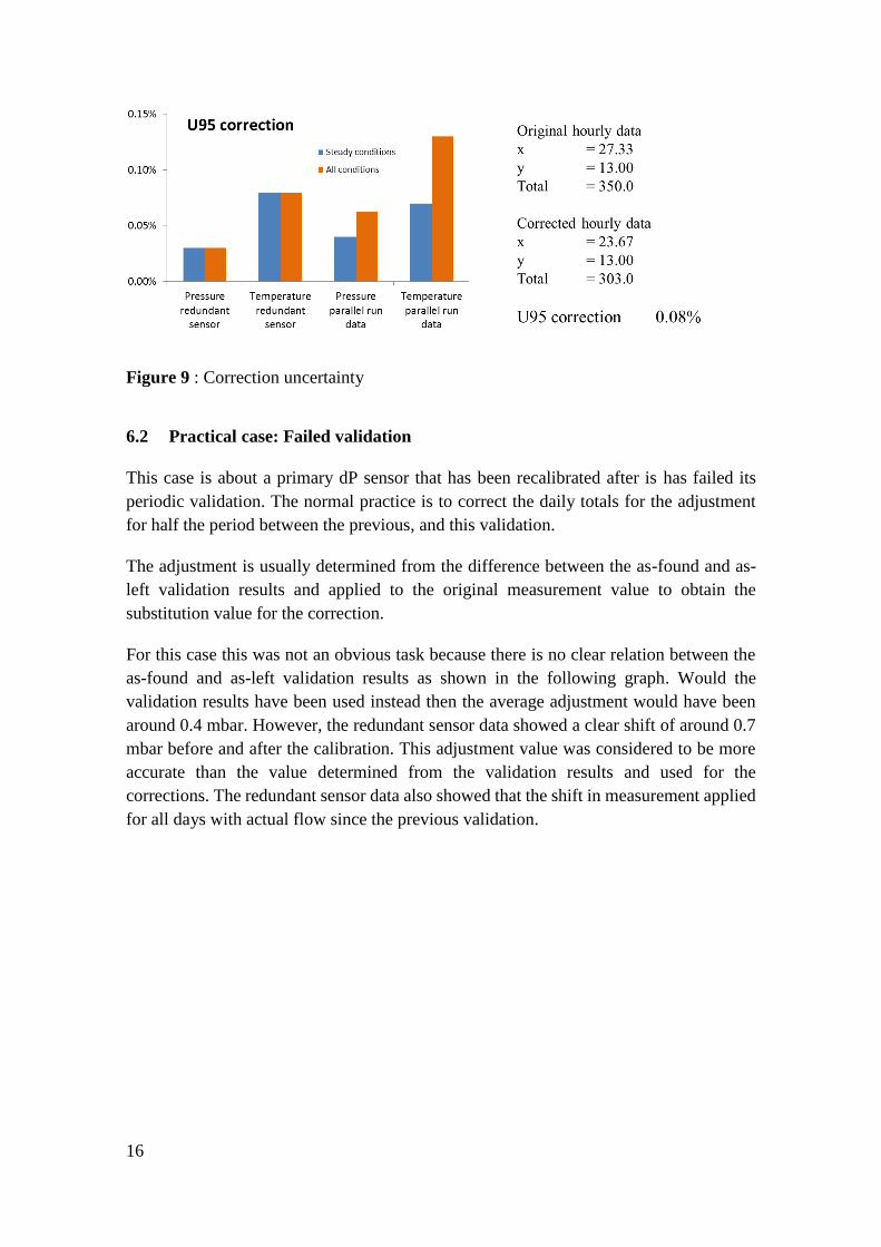
6.1.3 Correction uncertainty

The overall measurement is assumed to be within the contractual limit when all

measurements are operating within their tolerances and no failure has occurred. The

uncertainty of the corrected total is usually unknown though. A poor correction may even

increase the error.

An automated system has the additional benefit that the difference between the original

and the corrected totals can be determined in real-time, e.g. on an hourly basis. By

trending this difference over time for periods without a mismeasurement the correction

uncertainty can be quantified.

By knowing this uncertainty, it can be assured that corrections are only applied when the

corrected total is more accurate than the original total. Furthermore, it can be proved to

the customer; what the overall measurement uncertainty is even in case of a failure.

16

Figure 9 : Correction uncertainty

6.2 Practical case: Failed validation

This case is about a primary dP sensor that has been recalibrated after is has failed its

periodic validation. The normal practice is to correct the daily totals for the adjustment

for half the period between the previous, and this validation.

The adjustment is usually determined from the difference between the as-found and as-

left validation results and applied to the original measurement value to obtain the

substitution value for the correction.

For this case this was not an obvious task because there is no clear relation between the

as-found and as-left validation results as shown in the following graph. Would the

validation results have been used instead then the average adjustment would have been

around 0.4 mbar. However, the redundant sensor data showed a clear shift of around 0.7

mbar before and after the calibration. This adjustment value was considered to be more

accurate than the value determined from the validation results and used for the

corrections. The redundant sensor data also showed that the shift in measurement applied

for all days with actual flow since the previous validation.

17

Figure 10 : Failed validation case – Substitution value

The adjustment based on redundant sensor data resulted in the corrections shown by the

following graph. This shows that an automated system helps the user to make the best

possible correction based on all available information.

Figure 11 : Failed validation case – Error correction

6.3 Practical case: Shift in measurement

This case is about a primary temperature with a shift in measurement that was not detected

by the flow computer, but that became apparent when comparing the primary value with

both the substitution values.

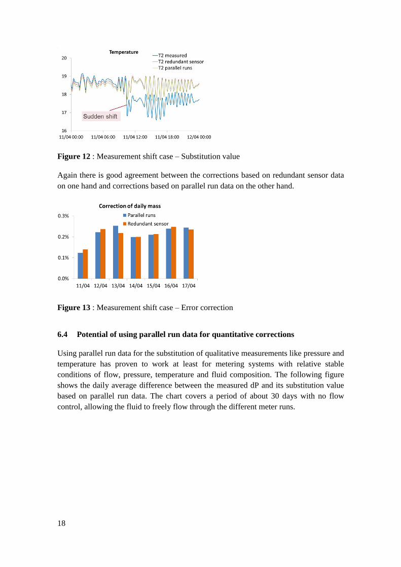
18

Figure 12 : Measurement shift case – Substitution value

Again there is good agreement between the corrections based on redundant sensor data

on one hand and corrections based on parallel run data on the other hand.

Figure 13 : Measurement shift case – Error correction

6.4 Potential of using parallel run data for quantitative corrections

Using parallel run data for the substitution of qualitative measurements like pressure and

temperature has proven to work at least for metering systems with relative stable

conditions of flow, pressure, temperature and fluid composition. The following figure

shows the daily average difference between the measured dP and its substitution value

based on parallel run data. The chart covers a period of about 30 days with no flow

control, allowing the fluid to freely flow through the different meter runs.

19

Figure 14 : Potential of parallel run data for quantitative corrections

The chart reveals the potential to use parallel run data to obtain reasonable accurate

substitution values for quantitative measurements as well, at least under stable and equal

flow conditions. However further analysis and field testing is required to either affirm or

reject this hypothesis.

7 CONCLUSION

For a fair trade of hydrocarbon products it is essential that measurements errors are

detected and corrected for. The accurate correction of a measurement error is not an

obvious task to do and requires both an accurate substitution of the faulty input value and

an accurate recalculation of the reported quantity.

Accurate substitution requires a value that more or less resembles the actual value during

the failure, ideally from a secondary sensor installed in the same meter run. If that is not

available then data from parallel meter runs would be the second best option especially at

steady flowing conditions.

The accurate recalculation requires data with a higher resolution than the quantity being

corrected. For instance for hourly totals data with a 5 minute interval is required to enable

accurate corrections, especially for a compressible fluid like a (liquefied) natural gas.

20

An automated system with consolidated data allows the operator to conveniently and

promptly deal with measurement errors and to generate accurate data for billing purposes

even in case of a measurement failure..

8 REFERENCES

(1) Determining a quantity of transported fluid - US 20130124113 A1 - Han van Dal

(2) API MPMS Chapter 21—Flow Measurement Using Electronic Metering Systems,

Section 1 – Electronic Gas Measurement