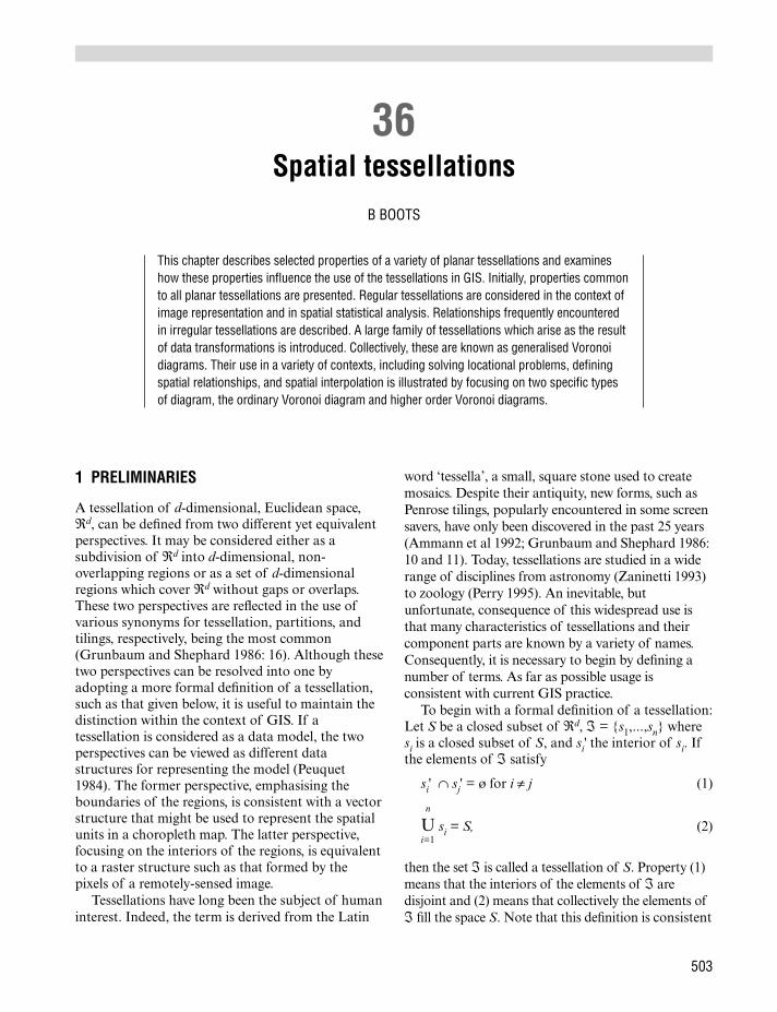
1 PRELIMINARIES

A tessellation of d-dimensional, Euclidean space,ℜd, can be defined from two different yet equivalentperspectives. It may be considered either as asubdivision of ℜd into d-dimensional, non-overlapping regions or as a set of d-dimensionalregions which cover ℜd without gaps or overlaps.These two perspectives are reflected in the use ofvarious synonyms for tessellation, partitions, andtilings, respectively, being the most common(Grunbaum and Shephard 1986: 16). Although thesetwo perspectives can be resolved into one byadopting a more formal definition of a tessellation,such as that given below, it is useful to maintain thedistinction within the context of GIS. If atessellation is considered as a data model, the twoperspectives can be viewed as different datastructures for representing the model (Peuquet1984). The former perspective, emphasising theboundaries of the regions, is consistent with a vectorstructure that might be used to represent the spatialunits in a choropleth map. The latter perspective,focusing on the interiors of the regions, is equivalentto a raster structure such as that formed by thepixels of a remotely-sensed image.

Tessellations have long been the subject of humaninterest. Indeed, the term is derived from the Latin

word ‘tessella’, a small, square stone used to createmosaics. Despite their antiquity, new forms, such asPenrose tilings, popularly encountered in some screensavers, have only been discovered in the past 25 years(Ammann et al 1992; Grunbaum and Shephard 1986:10 and 11). Today, tessellations are studied in a widerange of disciplines from astronomy (Zaninetti 1993)to zoology (Perry 1995). An inevitable, butunfortunate, consequence of this widespread use isthat many characteristics of tessellations and theircomponent parts are known by a variety of names.Consequently, it is necessary to begin by defining anumber of terms. As far as possible usage isconsistent with current GIS practice.

To begin with a formal definition of a tessellation:Let S be a closed subset of ℜd, ℑ = {s1,...,sn} wheresi is a closed subset of S, and si' the interior of si. Ifthe elements of ℑ satisfy

si' ∩ sj' = ø for i ≠ j (1)

n

U si = S, (2)i=1

then the set ℑ is called a tessellation of S. Property (1)means that the interiors of the elements of ℑ aredisjoint and (2) means that collectively the elements ofℑ fill the space S. Note that this definition is consistent

503

36Spatial tessellations

B BOOTS

This chapter describes selected properties of a variety of planar tessellations and examineshow these properties influence the use of the tessellations in GIS. Initially, properties commonto all planar tessellations are presented. Regular tessellations are considered in the context ofimage representation and in spatial statistical analysis. Relationships frequently encounteredin irregular tessellations are described. A large family of tessellations which arise as the resultof data transformations is introduced. Collectively, these are known as generalised Voronoidiagrams. Their use in a variety of contexts, including solving locational problems, definingspatial relationships, and spatial interpolation is illustrated by focusing on two specific typesof diagram, the ordinary Voronoi diagram and higher order Voronoi diagrams.

with practical applications such as thoseencountered in GIS, where the space underconsideration is a bounded region in Euclideanspace rather than the unbounded space itself (theusual situation in theoretical treatments). When d=2the tessellation is called a planar tessellation.Attention in this chapter is limited to planartessellations since these are those most commonlyencountered in GIS.

Planar tessellations are composed of threeelements of d (d≤2) dimensions (see Figure 1): cells(2-d), edges (1-d), and vertices (0-d). In GIS theseelements are usually referred to as polygons, lines(or arcs), and points respectively. In turn, each of thed (d>0)-dimensional elements are composed ofelements of (d-1) dimensions. Cells have sides (1-d)and corners (0-d), lines have end points (0-d). Atessellation, such as that in Figure 1, in which thecorners and sides of individual cells coincide withthe vertices and edges of the tessellation,respectively, is called an edge-to-edge tessellation.Individual rectangular cells arranged in a brick wallfashion would not constitute an edge-to-edgetessellation. Only edge-to-edge tessellations areconsidered here. A d-dimensional tessellation inwhich every s-dimensional element lies in theboundaries of (d–s+1) cells (0≤s≤d–1) is called anormal tessellation. Thus, in a normal planartessellation, each vertex is shared by three cells andeach edge is common to two cells.

A monohedral tessellation is one in which all thecells are of the same size and shape (e.g. thetessellation in Figure 2). More formally, each cell iscongruent (directly or reflectively) to one fixed set S.If ri denotes the number of edges meeting at the ithcorner of a cell in a monohedral tessellation, anisohedral tessellation is one in which the orderedsequence of values of ri is the same for every cell. Inshort, the cells are completely interchangeable sothat, as Bell and Holroyd (1991) note, ‘a bug whichwas put down in one of the [cells] and started toexplore the [tessellation] would find exactly the samearrangement of [cells] no matter which [cell] it wasoriginally deposited in’. More formally, all the cellsare equivalent under the symmetry group of thetessellation. Thus, the tessellation in Figure 3 isisohedral while that in Figure 2 is not.

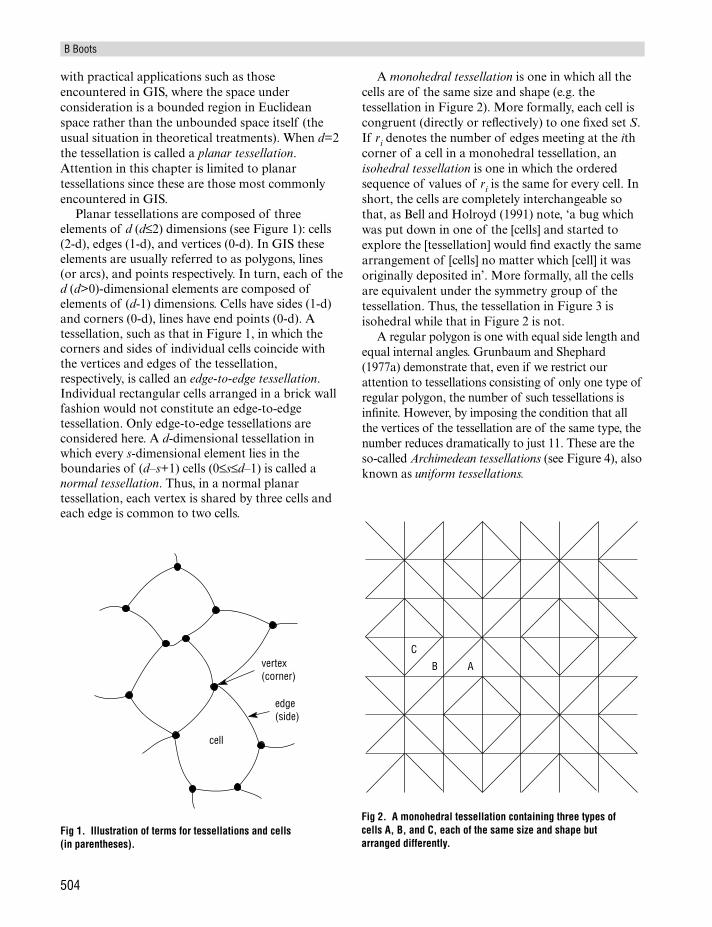
A regular polygon is one with equal side length andequal internal angles. Grunbaum and Shephard(1977a) demonstrate that, even if we restrict ourattention to tessellations consisting of only one type ofregular polygon, the number of such tessellations isinfinite. However, by imposing the condition that allthe vertices of the tessellation are of the same type, thenumber reduces dramatically to just 11. These are theso-called Archimedean tessellations (see Figure 4), alsoknown as uniform tessellations.

B Boots

504

Fig 1. Illustration of terms for tessellations and cells(in parentheses).

vertex(corner)

cell

edge(side)

Fig 2. A monohedral tessellation containing three types ofcells A, B, and C, each of the same size and shape butarranged differently.

C

B A

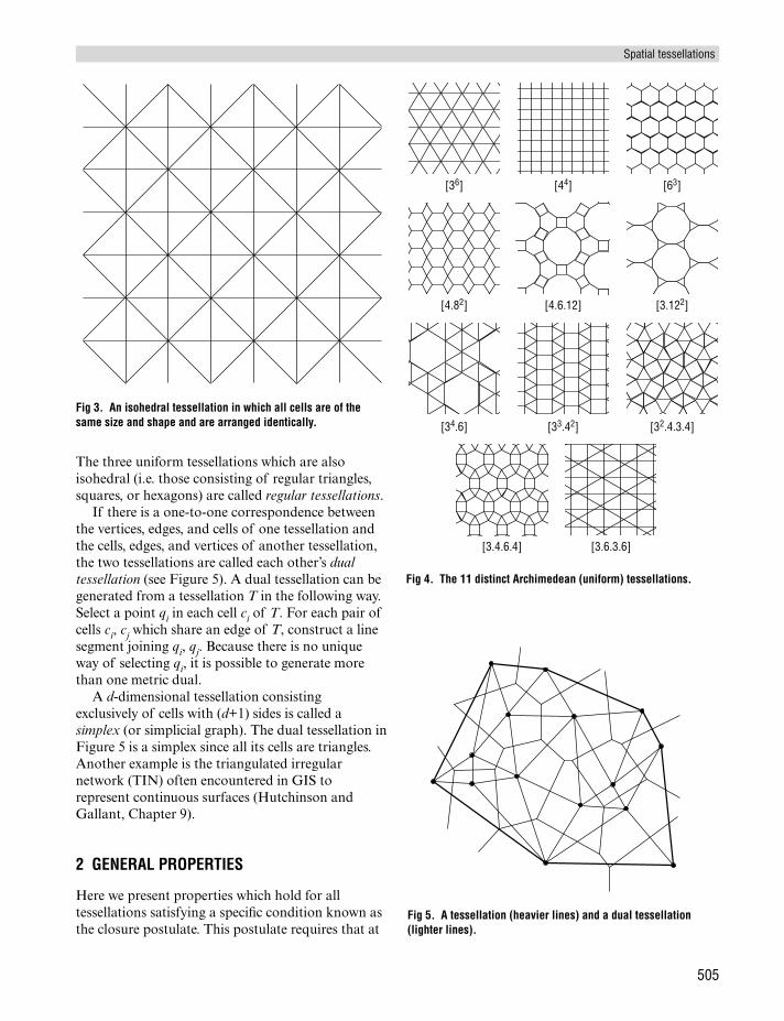
The three uniform tessellations which are alsoisohedral (i.e. those consisting of regular triangles,squares, or hexagons) are called regular tessellations.

If there is a one-to-one correspondence betweenthe vertices, edges, and cells of one tessellation andthe cells, edges, and vertices of another tessellation,the two tessellations are called each other’s dualtessellation (see Figure 5). A dual tessellation can begenerated from a tessellation T in the following way.Select a point qi in each cell ci of T. For each pair ofcells ci, cj which share an edge of T, construct a linesegment joining qi, qj. Because there is no uniqueway of selecting qi, it is possible to generate morethan one metric dual.

A d-dimensional tessellation consistingexclusively of cells with (d+1) sides is called asimplex (or simplicial graph). The dual tessellation inFigure 5 is a simplex since all its cells are triangles.Another example is the triangulated irregularnetwork (TIN) often encountered in GIS torepresent continuous surfaces (Hutchinson andGallant, Chapter 9).

2 GENERAL PROPERTIES

Here we present properties which hold for alltessellations satisfying a specific condition known asthe closure postulate. This postulate requires that at

Spatial tessellations

505

Fig 3. An isohedral tessellation in which all cells are of thesame size and shape and are arranged identically.

Fig 4. The 11 distinct Archimedean (uniform) tessellations.

[36] [44] [63]

[4.82] [4.6.12] [3.122]

[34.6] [33.42] [32.4.3.4]

[3.4.6.4] [3.6.3.6]

Fig 5. A tessellation (heavier lines) and a dual tessellation(lighter lines).

least two edges meet at every vertex and at least twocells meet at every edge. The elements in suchtessellations are related to each other throughEquation 3 derived by Schlaefli in 1852 as ageneralisation of a relationship first formulated byEuler one hundred years earlier (Loeb 1976):

j

∑ (–1)i Ni = 1 + (–1)j (3)i= 0

where Ni is the number of elements ofdimensionality i. For planar tessellations Equation 3reduces to:

N0 –N1 + N2 = 2 (4)

where N0, N1, N2 are the number of vertices, edges,and cells respectively. To satisfy the closurepostulate, if our tessellation is bounded, we mustinclude in our count of N2 an outside cell whosenumber of sides is equal to the number of edges onthe boundary of the tessellation.

If we define r=number of edges meeting at avertex and n=number of corners or sides of a cell, afurther equation can be derived from Equation 4,which reveals that we need only three parameters tospecify all of the characteristics of the tessellation.This equation is

1/r – 1/2 + 1/n = 1/N1 (5)

where r– and n– are the mean values of r and n,respectively. Equation 3 yields expressions for

N0 = 2N1/r (6)

and

N2 = 2N1/n (7)

The verification of Equations 3–7 is left as anexercise for the reader.

3 REGULAR TESSELLATIONS

This and the next section continue the exploration ofproperties of tessellations by looking in more detailat specific types of tessellations. However, theemphasis is shifted away from the propertiesthemselves towards an examination of how theymight influence the use of the tessellations withinspecific contexts in GIS. The first example involvesthe use of tessellations as spatial data models, inparticular in image representation.

To be useful in such a role tessellations shouldideally possess at least two properties (Ahuja 1983;Samet 1989):

1 be capable of generating an infinitely repetitivepattern, so that they can be used for images ofany size;

2 be infinitely (recursively) decomposable intoincreasingly finer patterns which, collectively,form a hierarchy, to allow for the representationof spatial features of arbitrarily fine resolution.

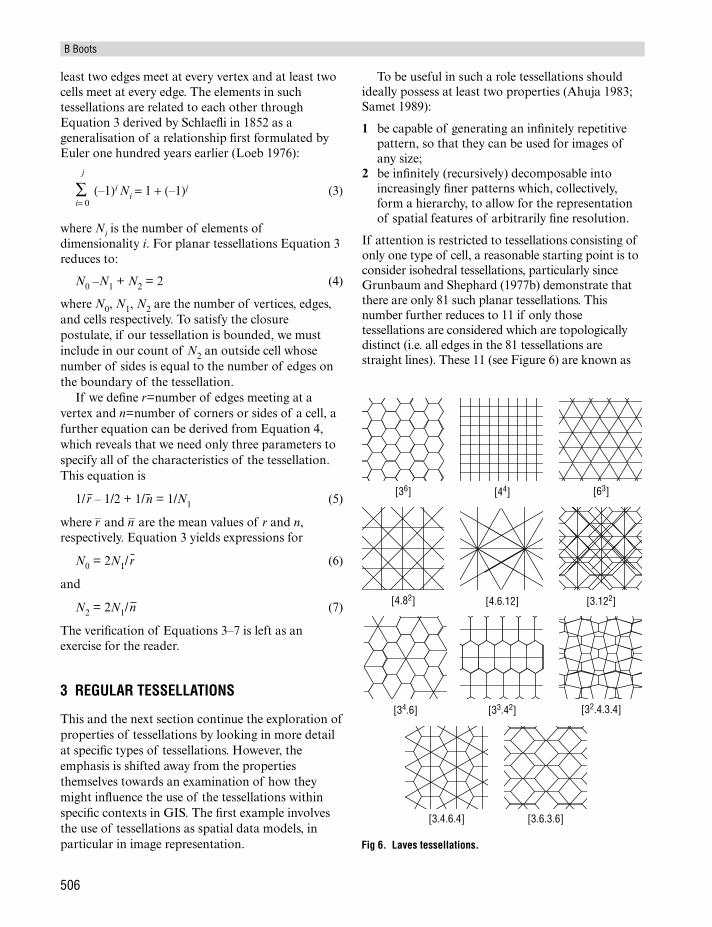
If attention is restricted to tessellations consisting ofonly one type of cell, a reasonable starting point is toconsider isohedral tessellations, particularly sinceGrunbaum and Shephard (1977b) demonstrate thatthere are only 81 such planar tessellations. Thisnumber further reduces to 11 if only thosetessellations are considered which are topologicallydistinct (i.e. all edges in the 81 tessellations arestraight lines). These 11 (see Figure 6) are known as

B Boots

506

Fig 6. Laves tessellations.

[36] [44] [63]

[4.82] [4.6.12] [3.122]

[34.6] [33.42] [32.4.3.4]

[3.4.6.4] [3.6.3.6]

Laves tessellations after the famous crystallographerFritz Laves. Laves tessellations may also be derived asduals of the uniform (Archimedean) tessellations inFigure 4. Note that three of the Laves tessellations areregular tessellations. To describe Laves tessellations weuse a notation based on the number of edges at thevertices of a constituent cell as they are visited in cyclicorder (see Figure 6). Thus, the three regulartessellations consisting of triangles, squares, andhexagons are labelled [63], [44] and [36] respectively.

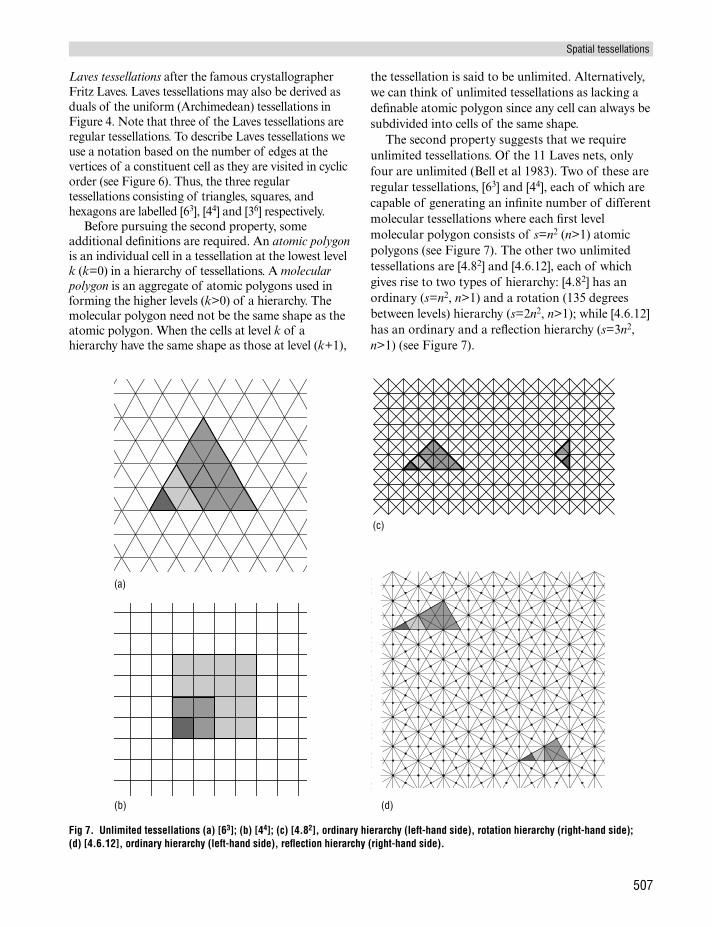
Before pursuing the second property, someadditional definitions are required. An atomic polygonis an individual cell in a tessellation at the lowest levelk (k=0) in a hierarchy of tessellations. A molecularpolygon is an aggregate of atomic polygons used informing the higher levels (k>0) of a hierarchy. Themolecular polygon need not be the same shape as theatomic polygon. When the cells at level k of ahierarchy have the same shape as those at level (k+1),

the tessellation is said to be unlimited. Alternatively,we can think of unlimited tessellations as lacking adefinable atomic polygon since any cell can always besubdivided into cells of the same shape.

The second property suggests that we requireunlimited tessellations. Of the 11 Laves nets, onlyfour are unlimited (Bell et al 1983). Two of these areregular tessellations, [63] and [44], each of which arecapable of generating an infinite number of differentmolecular tessellations where each first levelmolecular polygon consists of s=n2 (n>1) atomicpolygons (see Figure 7). The other two unlimitedtessellations are [4.82] and [4.6.12], each of whichgives rise to two types of hierarchy: [4.82] has anordinary (s=n2, n>1) and a rotation (135 degreesbetween levels) hierarchy (s=2n2, n>1); while [4.6.12]has an ordinary and a reflection hierarchy (s=3n2,n>1) (see Figure 7).

Spatial tessellations

507

Fig 7. Unlimited tessellations (a) [63]; (b) [44]; (c) [4.82], ordinary hierarchy (left-hand side), rotation hierarchy (right-hand side);(d) [4.6.12], ordinary hierarchy (left-hand side), reflection hierarchy (right-hand side).

(a)

(b)

(c)

(d)

Bell et al (1983, 1989) suggest additional tessellationproperties which are valuable in image processing andautomated cartography applications. Of these, the twomost important are uniform adjacency, whereby thedistances between the centroid of a given cell and thoseof neighbouring cells (whether edge or vertexneighbours) are the same, and uniform orientationwhich means that all cells have the same orientation.However, none of the four unlimited tessellationspossess the first property; [44] has two adjacencydistances, [63] three, [4.82] eight, and [4.6.12] 16.Further, only [44] displays uniform orientation. Thissituation leads to a reconsideration of the remainingregular tessellation [36] which possesses both propertieseven though it is not unlimited.

Although [36] cannot be decomposed beyond theatomic tessellation without changing the shape of the

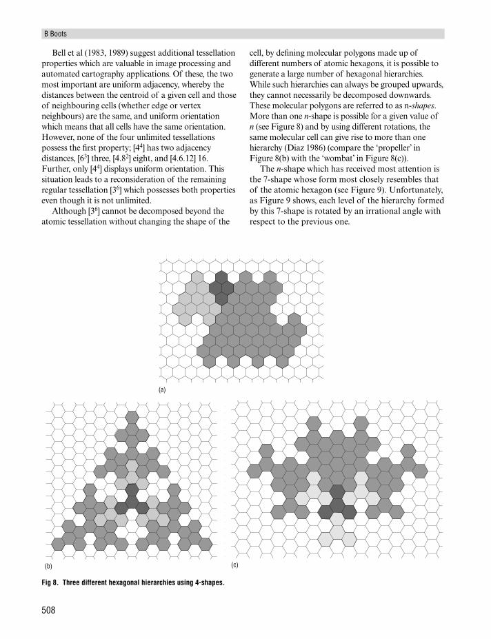
cell, by defining molecular polygons made up ofdifferent numbers of atomic hexagons, it is possible togenerate a large number of hexagonal hierarchies.While such hierarchies can always be grouped upwards,they cannot necessarily be decomposed downwards.These molecular polygons are referred to as n-shapes.More than one n-shape is possible for a given value ofn (see Figure 8) and by using different rotations, thesame molecular cell can give rise to more than onehierarchy (Diaz 1986) (compare the ‘propeller’ inFigure 8(b) with the ‘wombat’ in Figure 8(c)).

The n-shape which has received most attention isthe 7-shape whose form most closely resembles thatof the atomic hexagon (see Figure 9). Unfortunately,as Figure 9 shows, each level of the hierarchy formedby this 7-shape is rotated by an irrational angle withrespect to the previous one.

B Boots

508

Fig 8. Three different hexagonal hierarchies using 4-shapes.

(a)

(b) (c)

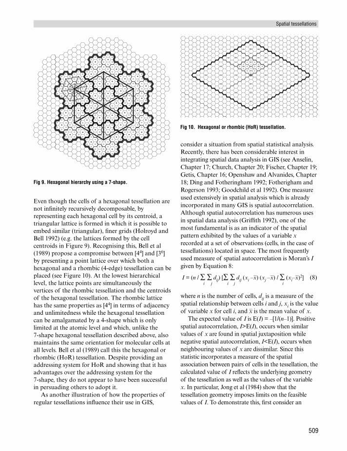
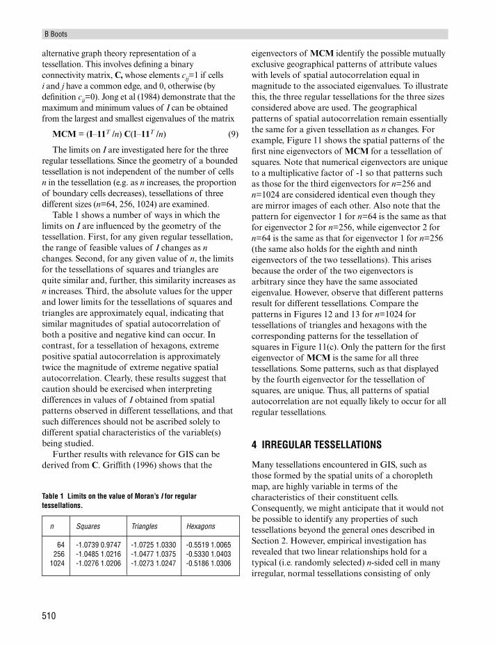
Even though the cells of a hexagonal tessellation arenot infinitely recursively decomposable, byrepresenting each hexagonal cell by its centroid, atriangular lattice is formed in which it is possible toembed similar (triangular), finer grids (Holroyd andBell 1992) (e.g. the lattices formed by the cellcentroids in Figure 9). Recognising this, Bell et al(1989) propose a compromise between [44] and [36]by presenting a point lattice over which both ahexagonal and a rhombic (4-edge) tessellation can beplaced (see Figure 10). At the lowest hierarchicallevel, the lattice points are simultaneously thevertices of the rhombic tessellation and the centroidsof the hexagonal tessellation. The rhombic latticehas the same properties as [44] in terms of adjacencyand unlimitedness while the hexagonal tessellationcan be amalgamated by a 4-shape which is onlylimited at the atomic level and which, unlike the7-shape hexagonal tessellation described above, alsomaintains the same orientation for molecular cells atall levels. Bell et al (1989) call this the hexagonal orrhombic (HoR) tessellation. Despite providing anaddressing system for HoR and showing that it hasadvantages over the addressing system for the7-shape, they do not appear to have been successfulin persuading others to adopt it.

As another illustration of how the properties ofregular tessellations influence their use in GIS,

consider a situation from spatial statistical analysis.Recently, there has been considerable interest inintegrating spatial data analysis in GIS (see Anselin,Chapter 17; Church, Chapter 20; Fischer, Chapter 19;Getis, Chapter 16; Openshaw and Alvanides, Chapter18; Ding and Fotheringham 1992; Fotherigham andRogerson 1993; Goodchild et al 1992). One measureused extensively in spatial analysis which is alreadyincorporated in many GIS is spatial autocorrelation.Although spatial autocorrelation has numerous usesin spatial data analysis (Griffith 1992), one of themost fundamental is as an indicator of the spatialpattern exhibited by the values of a variable xrecorded at a set of observations (cells, in the case oftessellations) located in space. The most frequentlyused measure of spatial autocorrelation is Moran’s Igiven by Equation 8:

I = (n / ∑ ∑ dij) [∑ ∑ dij (xi –x–) (xj –x–) / ∑ (xi–x–)2] (8)i j i j i

where n is the number of cells, dij is a measure of thespatial relationship between cells i and j, xi is the valueof variable x for cell i, and x– is the mean value of x.

The expected value of I is E(I) = –[1/(n–1)]. Positivespatial autocorrelation, I>E(I), occurs when similarvalues of x are found in spatial juxtaposition whilenegative spatial autocorrelation, I<E(I), occurs whenneighbouring values of x are dissimilar. Since thisstatistic incorporates a measure of the spatialassociation between pairs of cells in the tessellation, thecalculated value of I reflects the underlying geometryof the tessellation as well as the values of the variablex. In particular, Jong et al (1984) show that thetessellation geometry imposes limits on the feasiblevalues of I. To demonstrate this, first consider an

Spatial tessellations

509

Fig 9. Hexagonal hierarchy using a 7-shape.

Fig 10. Hexagonal or rhombic (HoR) tessellation.

alternative graph theory representation of atessellation. This involves defining a binaryconnectivity matrix, C, whose elements cij=1 if cellsi and j have a common edge, and 0, otherwise (bydefinition cii=0). Jong et al (1984) demonstrate that themaximum and minimum values of I can be obtainedfrom the largest and smallest eigenvalues of the matrix

MCM = (I–11T /n) C(I–11T /n) (9)

The limits on I are investigated here for the threeregular tessellations. Since the geometry of a boundedtessellation is not independent of the number of cellsn in the tessellation (e.g. as n increases, the proportionof boundary cells decreases), tessellations of threedifferent sizes (n=64, 256, 1024) are examined.

Table 1 shows a number of ways in which thelimits on I are influenced by the geometry of thetessellation. First, for any given regular tessellation,the range of feasible values of I changes as nchanges. Second, for any given value of n, the limitsfor the tessellations of squares and triangles arequite similar and, further, this similarity increases asn increases. Third, the absolute values for the upperand lower limits for the tessellations of squares andtriangles are approximately equal, indicating thatsimilar magnitudes of spatial autocorrelation ofboth a positive and negative kind can occur. Incontrast, for a tessellation of hexagons, extremepositive spatial autocorrelation is approximatelytwice the magnitude of extreme negative spatialautocorrelation. Clearly, these results suggest thatcaution should be exercised when interpretingdifferences in values of I obtained from spatialpatterns observed in different tessellations, and thatsuch differences should not be ascribed solely todifferent spatial characteristics of the variable(s)being studied.

Further results with relevance for GIS can bederived from C. Griffith (1996) shows that the

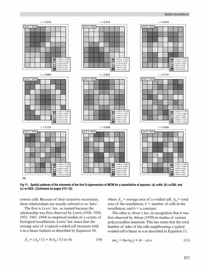
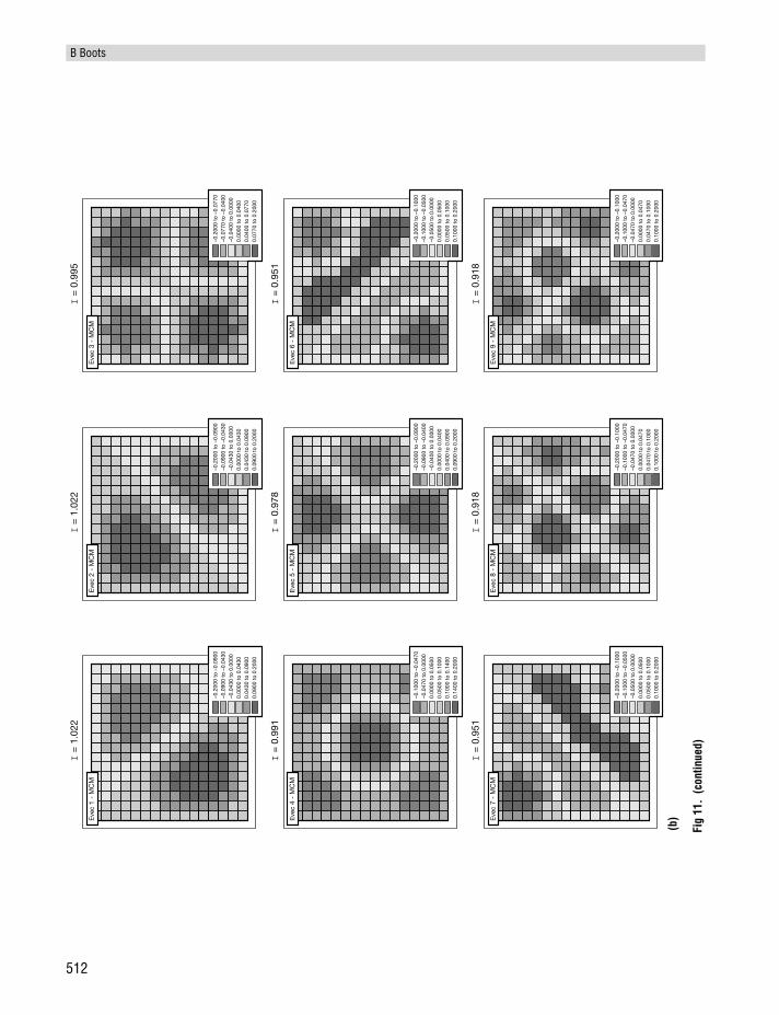
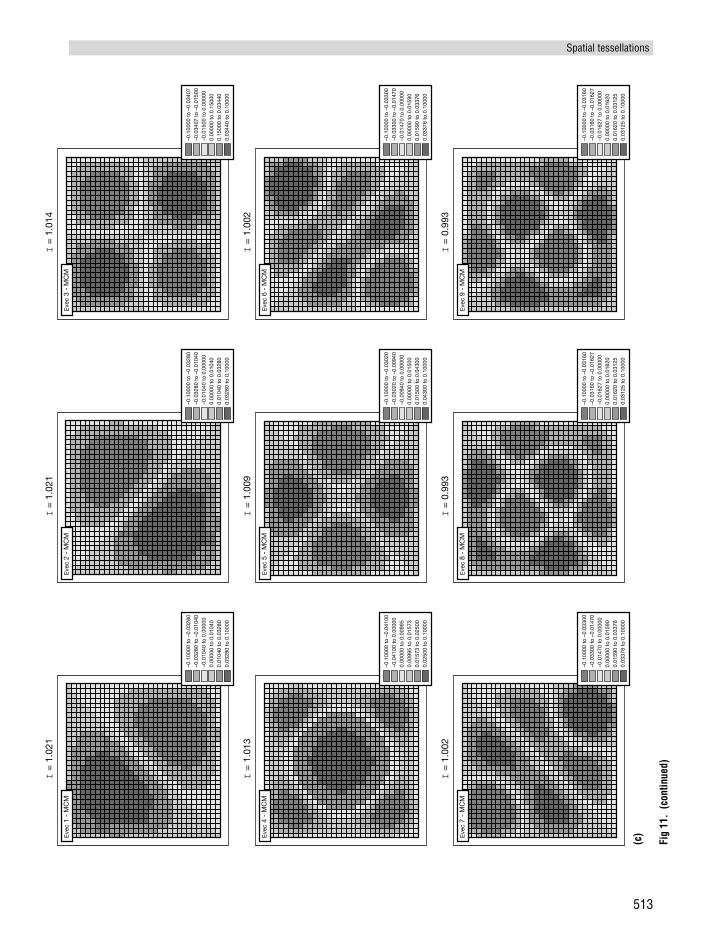
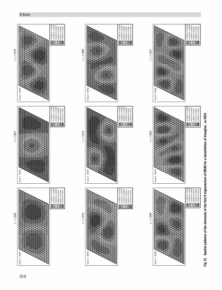
eigenvectors of MCM identify the possible mutuallyexclusive geographical patterns of attribute valueswith levels of spatial autocorrelation equal inmagnitude to the associated eigenvalues. To illustratethis, the three regular tessellations for the three sizesconsidered above are used. The geographicalpatterns of spatial autocorrelation remain essentiallythe same for a given tessellation as n changes. Forexample, Figure 11 shows the spatial patterns of thefirst nine eigenvectors of MCM for a tessellation ofsquares. Note that numerical eigenvectors are uniqueto a multiplicative factor of -1 so that patterns suchas those for the third eigenvectors for n=256 andn=1024 are considered identical even though theyare mirror images of each other. Also note that thepattern for eigenvector 1 for n=64 is the same as thatfor eigenvector 2 for n=256, while eigenvector 2 forn=64 is the same as that for eigenvector 1 for n=256(the same also holds for the eighth and nintheigenvectors of the two tessellations). This arisesbecause the order of the two eigenvectors isarbitrary since they have the same associatedeigenvalue. However, observe that different patternsresult for different tessellations. Compare thepatterns in Figures 12 and 13 for n=1024 fortessellations of triangles and hexagons with thecorresponding patterns for the tessellation ofsquares in Figure 11(c). Only the pattern for the firsteigenvector of MCM is the same for all threetessellations. Some patterns, such as that displayedby the fourth eigenvector for the tessellation ofsquares, are unique. Thus, all patterns of spatialautocorrelation are not equally likely to occur for allregular tessellations.

4 IRREGULAR TESSELLATIONS

Many tessellations encountered in GIS, such asthose formed by the spatial units of a choroplethmap, are highly variable in terms of thecharacteristics of their constituent cells.Consequently, we might anticipate that it would notbe possible to identify any properties of suchtessellations beyond the general ones described inSection 2. However, empirical investigation hasrevealed that two linear relationships hold for atypical (i.e. randomly selected) n-sided cell in manyirregular, normal tessellations consisting of only

B Boots

510

n Squares Triangles Hexagons

64 -1.0739 0.9747 -1.0725 1.0330 -0.5519 1.0065256 -1.0485 1.0216 -1.0477 1.0375 -0.5330 1.0403

1024 -1.0276 1.0206 -1.0273 1.0247 -0.5186 1.0306

Table 1 Limits on the value of Moran’s I for regulartessellations.

convex cells. Because of their extensive occurrence,these relationships are usually referred to as ‘laws’.

The first is Lewis’ law, so named because therelationship was first observed by Lewis (1928, 1930,1931, 1943, 1944) in empirical studies of a variety ofbiological tessellations. Lewis’ law states that theaverage area of a typical n-sided cell increases withn in a linear fashion as described by Equation 10:

A–

n = (A0 / C) + b(A0 / C) (n–6) (10)

where A–

n = average area of a n-sided cell; A0 = totalarea of the tessellation; C = number of cells in thetessellation; and b = a constant.

The other is Aboav’s law, in recognition that it wasfirst observed by Aboav (1970) in studies of variouspolycrystalline materials. This law states that the totalnumber of sides of the cells neighbouring a typicaln-sided cell is linear in n as described in Equation 11:

nmn = (6a+µ2) + (n– – a) n (11)

Spatial tessellations

511

Fig 11. Spatial patterns of the elements of the first 9 eigenvectors of MCM for a tessellation of squares: (a) n=64; (b) n=256; and(c) n=1024. (Continued on pages 512–13)

I = 0.724

Evec 7 - MCM

–0.2000 to –0.0800–0.0800 to 0.00000.3000 to 0.15000.1000 to 0.17000.1700 to 0.20000.2000 to 0.4000

I = 0.863

Evec 4 - MCM

–0.3000 to –0.1500–0.1500 to –0.0790–0.0790 to 0.00000.0000 to 0.07900.0790 to 0.15000.1500 to 0.3000

I = 0.975

Evec 1 - MCM

–0.3000 to –0.1500–0.1500 to –0.0800–0.0800 to 0.00000.0000 to 0.08000.0800 to 0.15000.1500 to 0.3000

I = 0.636

Evec 8 - MCM

–0.3000 to –0.1400–0.1400 to –0.1000–0.1000 to 0.00000.0000 to 0.10000.1000 to 0.14000.1400 to 0.3000

I = 0.823

Evec 5 - MCM

I = 0.975

Evec 2 - MCM

I = 0.636

Evec 9 - MCM

–0.3000 to –0.1790–0.1790 to –0.0890–0.0890 to 0.00000.0000 to –0.0890–0.0890 to –0.1790–0.1790 to –0.3000

I = 0.724

Evec 6 - MCM

–0.3000 to –0.1500–0.1500 to –0.0700–0.0700 to 0.00000.0000 to 0.07000.0700 to 0.15000.1500 to 0.3000

I = 0.876

Evec 3 - MCM

–0.3000 to –0.1500–0.1500 to –0.0790–0.0790 to 0.00000.0000 to 0.07900.0790 to 0.15000.1500 to 0.3000

–0.3000 to –0.1790–0.1790 to –0.0890–0.0890 to 0.00000.0000 to –0.0890–0.0890 to –0.1790–0.1790 to –0.3000

–0.3000 to –0.1500–0.1500 to –0.0800–0.0800 to 0.00000.0000 to 0.08000.0800 to 0.15000.1500 to 0.3000

(a)

Fig

11.

(con

tinue

d)

I =

0.9

51

Eve

c 7

- M

CM

–0.1

000

to –

0.04

70–0

.047

0 to

0.0

000

0.00

00 t

o 0.

0500

0.05

00 t

o 0.

1000

0.10

00 t

o 0.

1400

0.14

00 t

o 0.

2000

I =

0.9

91

Eve

c 4

- M

CM

–0.2

000

to –

0.09

00–0

.090

0 to

–0.

0430

–0.0

430

to 0

.000

00.

0000

to

0.04

300.

0430

to

0.09

000.

0900

to

0.20

00

I =

1.0

22

Eve

c 1

- M

CM

I =

0.9

18

Eve

c 8

- M

CM

–0.2

000

to –

0.09

00–0

.090

0 to

–0.

0400

–0.0

400

to 0

.000

00.

0000

to

0.04

000.

0400

to

0.09

000.

0900

to

0.20

00

I =

0.9

78

Eve

c 5

- M

CM

I =

1.0

22

Eve

c 2

- M

CM

I =

0.9

18

Eve

c 9

- M

CM

–0.2

000

to –

0.10

00–0

.100

0 to

–0.

0500

–0.0

500

to 0

.000

00.

0000

to

0.05

000.

0500

to

0.10

000.

1000

to

0.20

00

I =

0.9

51

Eve

c 6

- M

CM

–0.2

000

to –

0.07

70–0

.077

0 to

–0.

0400

–0.0

400

to 0

.000

00.

0000

to

0.04

000.

0400

to

0.07

700.

0770

to

0.20

00

I =

0.9

95

Eve

c 3

- M

CM

–0.2

000

to –

0.09

00–0

.090

0 to

–0.

0430

–0.0

430

to 0

.000

00.

0000

to

0.04

300.

0430

to

0.09

000.

0900

to

0.20

00

–0.2

000

to –

0.10

00–0

.100

0 to

–0.

0470

–0.0

470

to 0

.000

00.

0000

to

0.04

700.

0470

to

0.10

000.

1000

to

0.20

00

–0.2

000

to –

0.10

00–0

.100

0 to

–0.

0500

–0.0

500

to 0

.000

00.

0000

to

0.05

000.

0500

to

0.10

000.

1000

to

0.20

00

–0.2

000

to –

0.10

00–0

.100

0 to

–0.

0470

–0.0

470

to 0

.000

00.

0000

to

0.04

700.

0470

to

0.10

000.

1000

to

0.20

00

(b)

B Boots

512

Fig

11.

(con

tinue

d)

I =

1.0

02

Eve

c 7

- M

CM

–0.1

0000

to

–0.0

4100

–0.0

4100

to

0.00

000

0.00

000

to 0

.009

950.

0099

5 to

0.0

1573

0.01

573

to 0

.025

000.

0250

0 to

0.1

0000

I =

1.0

13

Eve

c 4

- M

CM

–0.1

0000

to

–0.0

3280

–0.0

3280

to

–0.0

1040

–0.0

1040

to

0.00

000

0.00

000

to 0

.010

400.

0104

0 to

0.0

3280

0.03

280

to 0

.100

00

I =

1.0

21

Eve

c 1

- M

CM

I =

0.9

93

Eve

c 8

- M

CM

–0.1

0000

to

–0.0

3020

–0.0

3020

to

–0.0

0940

–0.0

0940

to

0.00

000

0.00

000

to 0

.015

000.

0150

0 to

0.0

4300

0.04

300

to 0

.100

00

I =

1.0

09

Eve

c 5

- M

CM

I =

1.0

21

Eve

c 2

- M

CM

I =

0.9

93

Eve

c 9

- M

CM

–0.1

0000

to

–0.0

3300

–0.0

3300

to

–0.0

1470

–0.0

1470

to

0.00

000

0.00

000

to 0

.015

900.

0159

0 to

0.0

3376

0.03

376

to 0

.100

00

I =

1.0

02

Eve

c 6

- M

CM

–0.1

0000

to

–0.0

3407

–0.0

3407

to

–0.0

1500

–0.0

1500

to

0.00

000

0.00

000

to 0

.150

000.

1500

0 to

0.0

3440

0.03

440

to 0

.100

00

I =

1.0

14

Eve

c 3

- M

CM

–0.1

0000

to

–0.0

3280

–0.0

3280

to

–0.0

1040

–0.0

1040

to

0.00

000

0.00

000

to 0

.010

400.

0104

0 to

0.0

3280

0.03

280

to 0

.100

00

–0.1

0000

to

–0.0

3160

–0.0

3160

to

–0.0

1627

–0.0

1627

to

0.00

000

0.00

000

to 0

.016

200.

0162

0 to

0.0

3125

0.03

125

to 0

.100

00

–0.1

0000

to

–0.0

3300

–0.0

3300

to

–0.0

1470

–0.0

1470

to

0.00

000

0.00

000

to 0

.015

900.

0159

0 to

0.0

3376

0.03

376

to 0

.100

00

–0.1

0000

to

–0.0

3160

–0.0

3160

to

–0.0

1627

–0.0

1627

to

0.00

000

0.00

000

to 0

.016

200.

0162

0 to

0.0

3125

0.03

125

to 0

.100

00

(c)

Spatial tessellations

513

Fig

12.

Spat

ial p

atte

rns

of th

e el

emen

ts o

f the

firs

t 9 e

igen

vect

ors

of M

CM fo

r a te

ssel

latio

n of

tria

ngle

s,n

=102

4.

I =

1.0

25

Eve

c 1

- M

CM

–0.1

0000

to

–0.0

4100

–0.0

4100

to

–0.0

2000

–0.0

2000

to

–0.0

0000

0.00

000

to 0

.020

000.

0200

0 to

0.0

4100

0.04

100

to 0

.100

00

I =

1.0

15

Eve

c 4

- M

CM

–0.1

0000

to

–0.0

5120

–0.0

5120

to

–0.0

2570

–0.0

2570

to

0.00

000

0.00

000

to 0

.025

700.

0257

0 to

0.0

5120

0.05

120

to 0

.100

00

I =

1.0

08

Eve

c 7

- M

CM

–0.1

0000

to

–0.0

4900

–0.0

4900

to

–0.0

2400

–0.0

2400

to

0.00

000

0.00

000

to 0

.024

000.

0240

0 to

0.0

4900

0.04

900

to 0

.100

00

I =

1.0

21

Eve

c 2

- M

CM

I =

1.0

13

Eve

c 5

- M

CM

–0.1

0000

to

–0.0

6900

–0.0

6900

to

–0.0

4600

–0.0

4600

to

–0.0

2290

–0.0

2290

to

0.00

000

0.00

000

to 0

.023

000.

0230

0 to

0.1

0000

I =

1.0

02

Eve

c 8

- M

CM

–0.1

0000

to

–0.0

4800

–0.0

4800

to

–0.0

2410

–0.0

2410

to

0.00

000

0.00

000

to 0

.024

100.

0241

0 to

0.0

4800

0.04

800

to 0

.100

00

I =

1.0

16

Eve

c 3

- M

CM

–0.1

0000

to

–0.0

4460

–0.0

4460

to

–0.0

2230

–0.0

2230

to

0.00

000

0.00

000

to 0

.022

300.

0223

0 to

0.0

4460

0.04

460

to 0

.100

00

I =

1.0

09

Eve

c 6

- M

CM

–0.1

0000

to

–0.0

2660

–0.0

2660

to

0.00

000

0.00

000

to 0

.026

600.

0266

0 to

0.0

5300

0.05

300

to 0

.079

900.

0799

0 to

0.1

0000

I =

1.0

01

Eve

c 9

- M

CM

–0.1

0000

to

–0.0

5100

–0.0

5100

to

–0.0

2600

–0.0

2600

to

0.00

000

0.00

000

to 0

.026

000.

0260

0 to

0.0

5000

0.05

000

to 0

.100

00

–0.1

0000

to

–0.0

7300

–0.0

7300

to

–0.0

4900

–0.0

4900

to

–0.0

2430

–0.0

2430

to

0.00

000

0.00

000

to 0

.024

300.

0243

0 to

0.1

0000

514

B Boots

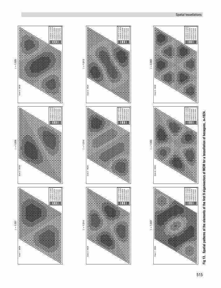
Fig

13.

Spat

ial p

atte

rns

of th

e el

emen

ts o

f the

firs

t 9 e

igen

vect

ors

of M

CM fo

r a te

ssel

latio

n of

hex

agon

s, n

=102

4.

Eve

c 1

- M

CM

–0.1

0000

to

–0.0

4300

–0.0

4300

to

–0.0

2140

–0.0

2140

to

0.00

000

0.00

000

to 0

.021

400.

0214

0 to

0.0

4300

0.04

300

to 0

.100

00

I =

1.0

31

Eve

c 2

- M

CM

–0.1

0000

to

–0.0

4800

–0.0

4800

to

–0.0

2370

–0.0

2370

to

0.00

000

0.00

000

to 0

.023

700.

0237

0 to

0.0

4800

0.04

800

to 0

.100

00

I =

1.0

26

Eve

c 4

- M

CM

–0.1

0000

to

–0.0

4500

–0.0

4500

to

–0.0

2300

–0.0

2300

to

0.00

000

–0.0

0000

to

0.02

300

0.02

300

to 0

.450

00.

0450

0 to

0.1

0000

I =

1.0

14I

= 1

.014

I =

0.9

93I

= 1

.003

Eve

c 8

- M

CM

–0.1

0000

to

–0.0

4600

–0.0

4600

to

–0.0

2300

–0.0

2300

to

0.00

000

0.00

000

to 0

.023

000.

0230

0 to

0.0

4600

0.04

600

to 0

.100

00

I =

1.0

03

Eve

c 5

- M

CM

–0.1

0000

to

–0.0

5100

–0.0

5100

to

–0.0

2550

–0.0

2550

to

0.00

000

0.00

000

to 0

.025

500.

0255

0 to

0.0

5100

0.05

100

to 0

.100

00

Eve

c 3

- M

CM

–0.1

0000

to

–0.0

4500

–0.0

4500

to

–0.0

2300

–0.0

2300

to

0.00

000

0.00

000

to 0

.022

000.

0220

0 to

0.0

4400

0.04

400

to 0

.100

00

I =

1.0

25

Eve

c 6

- M

CM

–0.1

0000

to

–0.0

4500

–0.0

4500

to

–0.0

2300

–0.0

2300

to

0.00

000

0.00

000

to 0

.023

000.

0230

0 to

0.0

4700

0.04

700

to 0

.100

00

I =

1.0

13

Eve

c 7

- M

CM

Eve

c 9

- M

CM

–0.1

0000

to

–0.0

4300

–0.0

4300

to

–0.0

2140

–0.0

2140

to

0.00

000

0.00

000

to 0

.021

400.

0214

0 to

0.0

4300

0.04

300

to 0

.100

00

–0.1

0000

to

–0.0

7200

–0.0

7200

to

–0.0

4800

–0.0

4800

to

–0.0

2300

–0.0

2300

to

0.00

000

0.00

000

to 0

.023

000.

0230

0 to

0.1

0000

515

Spatial tessellations

where mn = number of sides of a randomly chosenneighbour of a typical n-sided cell; n– = mean value of n for the tessellation;µ2 = n– 2 – (n–)2 ;n–2 = mean value of n2 for the tessellation.

This law implies that, on average, cells with fewsides are likely to be adjacent to those with manysides, and vice versa.

No satisfactory explanations for the laws have yetbeen found. Most arguments involve an approachwhich maximises the entropy of pn, the distribution ofn for the tessellation, subject to a minimal set ofconstraints (Chiu 1995; Peshkin et al 1991; Rivier1985, 1986, 1990, 1991, 1993, 1994; Rivier andLissowski 1982). Both laws are seen as the most likelyrelationships to arise by chance in the absence of anyother constraints.

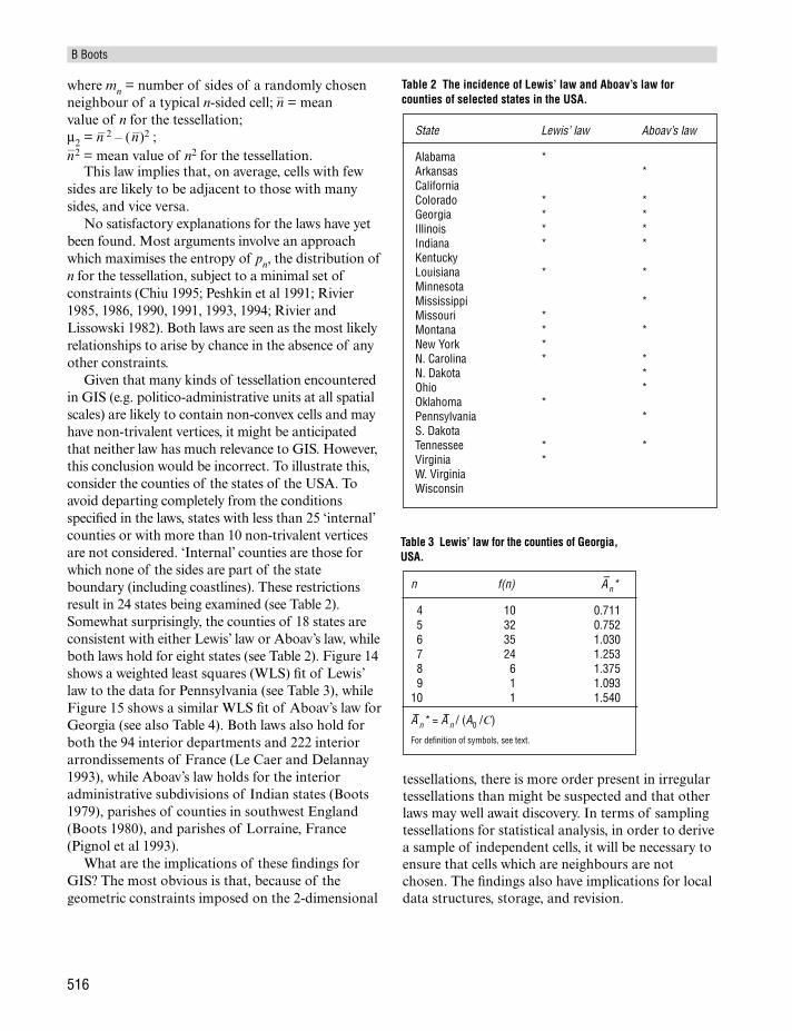
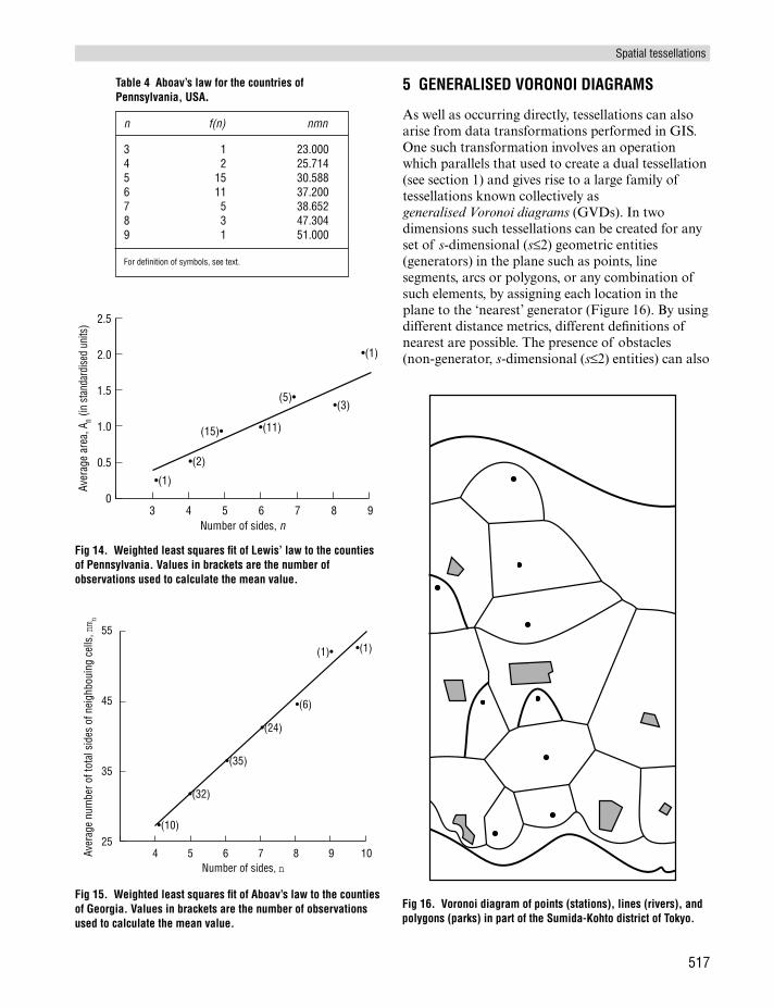
Given that many kinds of tessellation encounteredin GIS (e.g. politico-administrative units at all spatialscales) are likely to contain non-convex cells and may have non-trivalent vertices, it might be anticipatedthat neither law has much relevance to GIS. However,this conclusion would be incorrect. To illustrate this,consider the counties of the states of the USA. Toavoid departing completely from the conditionsspecified in the laws, states with less than 25 ‘internal’counties or with more than 10 non-trivalent verticesare not considered. ‘Internal’ counties are those forwhich none of the sides are part of the stateboundary (including coastlines). These restrictionsresult in 24 states being examined (see Table 2).Somewhat surprisingly, the counties of 18 states areconsistent with either Lewis’ law or Aboav’s law, whileboth laws hold for eight states (see Table 2). Figure 14shows a weighted least squares (WLS) fit of Lewis’law to the data for Pennsylvania (see Table 3), whileFigure 15 shows a similar WLS fit of Aboav’s law forGeorgia (see also Table 4). Both laws also hold forboth the 94 interior departments and 222 interiorarrondissements of France (Le Caer and Delannay1993), while Aboav’s law holds for the interioradministrative subdivisions of Indian states (Boots1979), parishes of counties in southwest England(Boots 1980), and parishes of Lorraine, France(Pignol et al 1993).

What are the implications of these findings forGIS? The most obvious is that, because of thegeometric constraints imposed on the 2-dimensional

tessellations, there is more order present in irregulartessellations than might be suspected and that otherlaws may well await discovery. In terms of samplingtessellations for statistical analysis, in order to derivea sample of independent cells, it will be necessary toensure that cells which are neighbours are notchosen. The findings also have implications for localdata structures, storage, and revision.

B Boots

516

State Lewis’ law Aboav’s law

Alabama *Arkansas *California Colorado * *Georgia * *Illinois * *Indiana * *KentuckyLouisiana * *MinnesotaMississippi *Missouri *Montana * *New York *N. Carolina * *N. Dakota *Ohio *Oklahoma *Pennsylvania *S. DakotaTennessee * *Virginia *W. VirginiaWisconsin

n f(n) A–

n*

4 10 0.7115 32 0.7526 35 1.0307 24 1.2538 6 1.3759 1 1.093

10 1 1.540

A–n* = A–n / (A0 /C)

For definition of symbols, see text.

Table 2 The incidence of Lewis’ law and Aboav’s law forcounties of selected states in the USA.

Table 3 Lewis’ law for the counties of Georgia,USA.

5 GENERALISED VORONOI DIAGRAMS

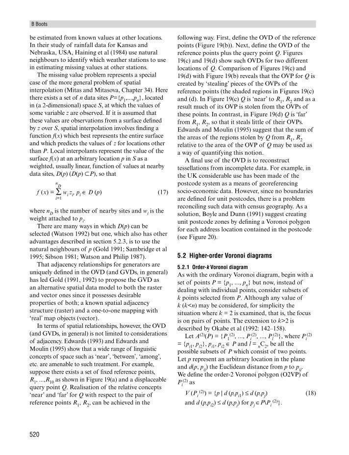
As well as occurring directly, tessellations can alsoarise from data transformations performed in GIS.One such transformation involves an operationwhich parallels that used to create a dual tessellation(see section 1) and gives rise to a large family oftessellations known collectively as generalised Voronoi diagrams (GVDs). In twodimensions such tessellations can be created for anyset of s-dimensional (s≤2) geometric entities(generators) in the plane such as points, linesegments, arcs or polygons, or any combination ofsuch elements, by assigning each location in theplane to the ‘nearest’ generator (Figure 16). By usingdifferent distance metrics, different definitions ofnearest are possible. The presence of obstacles(non-generator, s-dimensional (s≤2) entities) can also

Spatial tessellations

517

Fig 16. Voronoi diagram of points (stations), lines (rivers), andpolygons (parks) in part of the Sumida-Kohto district of Tokyo.

Fig 14. Weighted least squares fit of Lewis’ law to the countiesof Pennsylvania. Values in brackets are the number ofobservations used to calculate the mean value.

3 4 5 6 7 8 90

0.5

1.0

1.5

2.0

2.5

Aver

age

area

, An (

in s

tand

ardi

sed

units

)

Number of sides, n

•(1)

•(2)

(15)• •(11)

(5)••(3)

•(1)

Fig 15. Weighted least squares fit of Aboav’s law to the countiesof Georgia. Values in brackets are the number of observationsused to calculate the mean value.

4 5 6 7 8 9 1025

35

45

55

Aver

age

num

ber o

f tot

al s

ides

of n

eigh

boui

ng c

ells

, nm n

Number of sides, n

•(10)

(1)•

•(32)

•(35)

•(24)

•(6)

•(1)

n f(n) nmn

3 1 23.0004 2 25.7145 15 30.5886 11 37.2007 5 38.6528 3 47.3049 1 51.000

For definition of symbols, see text.

Table 4 Aboav’s law for the countries ofPennsylvania, USA.

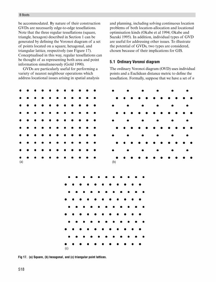
be accommodated. By nature of their constructionGVDs are necessarily edge-to-edge tessellations.Note that the three regular tessellations (square,triangle, hexagon) described in Section 1 can begenerated by defining the Voronoi diagram of a setof points located on a square, hexagonal, andtriangular lattice, respectively (see Figure 17).Conceptualised in this way, regular tessellations canbe thought of as representing both area and pointinformation simultaneously (Gold 1990).

GVDs are particularly useful for performing avariety of nearest neighbour operations whichaddress locational issues arising in spatial analysis

and planning, including solving continuous locationproblems of both location-allocation and locationaloptimisation kinds (Okabe et al 1994; Okabe andSuzuki 1995). In addition, individual types of GVDare useful for addressing other issues. To illustratethe potential of GVDs, two types are considered,chosen because of their implications for GIS.

5.1 Ordinary Voronoi diagram

The ordinary Voronoi diagram (OVD) uses individualpoints and a Euclidean distance metric to define thetessellation. Formally, suppose that we have a set of n

B Boots

518

Fig 17. (a) Square, (b) hexagonal, and (c) triangular point lattices.

(a) (b)

(c)

(2 ≤ n ≤ ∞) distinct points (generators), P = {p1,...,pn},located in a finite region S in 2-dimensional space ℜ2.To avoid complicated treatment, assume that S isconvex. Let d (p, pi) be Euclidean distance betweenlocation p and generator pi.

We define the region given by:

V (pi) = {p | p∈S; d (p, pi) ≤ d (p, pj), j ≠ i, j=1,...,n} (12)

as the ordinary Voronoi polygon (OVP) associatedwith pi and the set given by

υ (P) = {V (p1),..., V (pn)} (13)

as the OVD of P.Thus, the interior of V(pi) consists of all locations

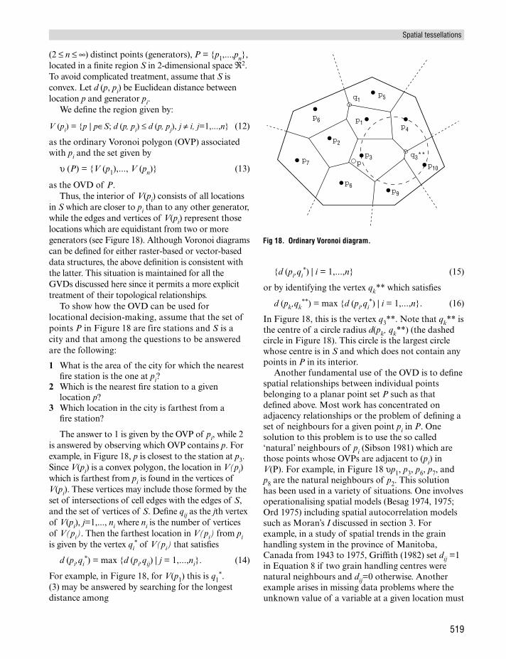
in S which are closer to pi than to any other generator,while the edges and vertices of V(pi) represent thoselocations which are equidistant from two or moregenerators (see Figure 18). Although Voronoi diagramscan be defined for either raster-based or vector-baseddata structures, the above definition is consistent withthe latter. This situation is maintained for all theGVDs discussed here since it permits a more explicittreatment of their topological relationships.

To show how the OVD can be used forlocational decision-making, assume that the set ofpoints P in Figure 18 are fire stations and S is acity and that among the questions to be answeredare the following:

1 What is the area of the city for which the nearestfire station is the one at pi?

2 Which is the nearest fire station to a givenlocation p?

3 Which location in the city is farthest from afire station?

The answer to 1 is given by the OVP of pi, while 2is answered by observing which OVP contains p. Forexample, in Figure 18, p is closest to the station at p3.Since V(pi) is a convex polygon, the location in V(pi)which is farthest from pi is found in the vertices ofV(pi). These vertices may include those formed by theset of intersections of cell edges with the edges of S,and the set of vertices of S. Define qij as the jth vertexof V(pi), j=1,..., ni where ni is the number of verticesof V(pi). Then the farthest location in V(pi) from piis given by the vertex qi

* of V(pi) that satisfies

d (pi,qi*) = max {d (pi,qij) | j = 1,...,ni}. (14)

For example, in Figure 18, for V(p1) this is q1*.

(3) may be answered by searching for the longestdistance among

{d (pi,qi*) | i = 1,...,n} (15)

or by identifying the vertex qk** which satisfies

d (pk,qk**) = max {d (pi,qi

*) | i = 1,...,n}. (16)

In Figure 18, this is the vertex q3**. Note that qk** isthe centre of a circle radius d(pk, qk**) (the dashedcircle in Figure 18). This circle is the largest circlewhose centre is in S and which does not contain anypoints in P in its interior.

Another fundamental use of the OVD is to definespatial relationships between individual pointsbelonging to a planar point set P such as thatdefined above. Most work has concentrated onadjacency relationships or the problem of defining aset of neighbours for a given point pi in P. Onesolution to this problem is to use the so called‘natural’ neighbours of pi (Sibson 1981) which arethose points whose OVPs are adjacent to (pi) inV(P). For example, in Figure 18 υp1, p3, p6, p7, andp8 are the natural neighbours of p2. This solutionhas been used in a variety of situations. One involvesoperationalising spatial models (Besag 1974, 1975;Ord 1975) including spatial autocorrelation modelssuch as Moran’s I discussed in section 3. Forexample, in a study of spatial trends in the grainhandling system in the province of Manitoba,Canada from 1943 to 1975, Griffith (1982) set dij =1in Equation 8 if two grain handling centres werenatural neighbours and dij=0 otherwise. Anotherexample arises in missing data problems where theunknown value of a variable at a given location must

Spatial tessellations

519

Fig 18. Ordinary Voronoi diagram.

p6

p7

p2

p6

p3

p1

p5

p4

p10

p9

q1

pq3**

be estimated from known values at other locations.In their study of rainfall data for Kansas andNebraska, USA, Haining et al (1984) use naturalneighbours to identify which weather stations to usein estimating missing values at other stations.

The missing value problem represents a specialcase of the more general problem of spatialinterpolation (Mitas and Mitasova, Chapter 34). Herethere exists a set of n data sites P={p1,...,pn}, locatedin (a 2-dimensional) space S, at which the values ofsome variable z are observed. If it is assumed thatthese values are observations from a surface definedby z over S, spatial interpolation involves finding afunction f(x) which best represents the entire surfaceand which predicts the values of z for locations otherthan P. Local interpolants represent the value of thesurface f(x) at an arbitrary location p in S as aweighted, usually linear, function of values at nearbydata sites, D(p) (D(p) �P), so that

nD

f (x) = ∑ wi zi, pi ∈ D (p) (17)i=1

where nD is the number of nearby sites and wi is theweight attached to pi.

There are many ways in which D(p) can beselected (Watson 1992) but one, which also has otheradvantages described in section 5.2.3, is to use thenatural neighbours of p (Gold 1991; Sambridge et al1995; Sibson 1981; Watson and Philip 1987).

That adjacency relationships for generators areuniquely defined in the OVD (and GVDs, in general)has led Gold (1991, 1992) to propose the GVD asan alternative spatial data model to both the rasterand vector ones since it possesses desirableproperties of both; a known spatial adjacencystructure (raster) and a one-to-one mapping with‘real’ map objects (vector).

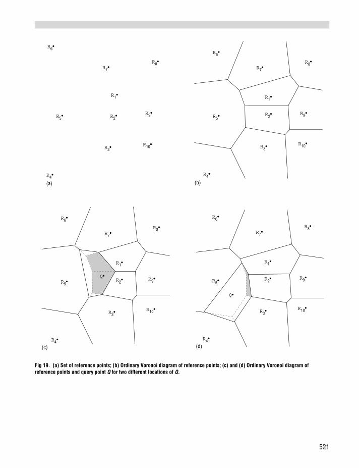
In terms of spatial relationships, however, the OVD(and GVDs, in general) is not limited to considerationsof adjacency. Edwards (1993) and Edwards andMoulin (1995) show that a wide range of linguisticconcepts of space such as ‘near’, ‘between’, ‘among’,etc. are amenable to such treatment. For example,suppose there exists a set of fixed reference points,R1, ...,R10 as shown in Figure 19(a) and a displaceablequery point Q. Realisation of the relative concepts‘near’ and ‘far’ for Q with respect to the pair ofreference points R1, R2, can be achieved in the

following way. First, define the OVD of the referencepoints (Figure 19(b)). Next, define the OVD of thereference points plus the query point Q. Figures19(c) and 19(d) show such OVDs for two differentlocations of Q. Comparison of Figures 19(c) and19(d) with Figure 19(b) reveals that the OVP for Q iscreated by ‘stealing’ pieces of the OVPs of thereference points (the shaded regions in Figures 19(c)and (d). In Figure 19(c) Q is ‘near’ to R1, R2 and as aresult much of its OVP is stolen from the OVPs ofthese points. In contrast, in Figure 19(d) Q is ‘far’from R1, R2, so that it steals little of their OVPs.Edwards and Moulin (1995) suggest that the sum ofthe areas of the regions stolen by Q from R1, R2relative to the area of the OVP of Q may be used asa way of quantifying this notion.

A final use of the OVD is to reconstructtessellations from incomplete data. For example, inthe UK considerable use has been made of thepostcode system as a means of georeferencingsocio-economic data. However, since no boundariesare defined for unit postcodes, there is a problemreconciling such data with census geography. As asolution, Boyle and Dunn (1991) suggest creatingunit postcode zones by defining a Voronoi polygonfor each address location contained in the postcode(see Figure 20).

5.2 Higher-order Voronoi diagrams

5.2.1 Order-k Voronoi diagramAs with the ordinary Voronoi diagram, begin with aset of points P = {p1, ..., pn} but now, instead ofdealing with individual points, consider subsets ofk points selected from P. Although any value ofk (k<n) may be considered, for simplicity thesituation where k = 2 is examined, that is, the focusis on pairs of points. The extension to k>2 isdescribed by Okabe et al (1992: 142–158).

Let A(2)(P) = {P1(2), ..., Pi

(2), ..., Pl(2)}, where Pi

(2)

= {pi1, pi2}, pi1, pi2 ∈ P and l = nC2, be all thepossible subsets of P which consist of two points.Let p represent an arbitrary location in the planeand d(p, pij) the Euclidean distance from p to pij.We define the order-2 Voronoi polygon (O2VP) ofPi

(2) as

V (Pi (2)) = {p | d (p,pi1) ≤ d (p,pj) (18)

and d (p,pi2) ≤ d (p,pj) for pj ∈P\Pi (2)}.

B Boots

520

521

Fig 19. (a) Set of reference points; (b) Ordinary Voronoi diagram of reference points; (c) and (d) Ordinary Voronoi diagram ofreference points and query point Q for two different locations of Q.

R5•

(a)

R6•

R7•R8•

R1•

R9•R2•

R10•R3•

R4•(b)

R5•

R6•

R7•R8•

R1•

R9•R2•

R10•R3•

R4•

Q•

(c)

R5•

R6•

R7•R8•

R1•

R9•R2•

R10•R3•

R4•

Q•

(d)

R5•

R6•

R7•R8•

R1•

R9•R2•

R10•R3•

R4•

Thus, V(Pi(2)) consists of all locations for which

either pi1 or pi2 is the first or second nearest point.The set

υ (A(2) (P)) = υ(2) = {V (P1(2)), ..., V (Pl

(2))} (19)

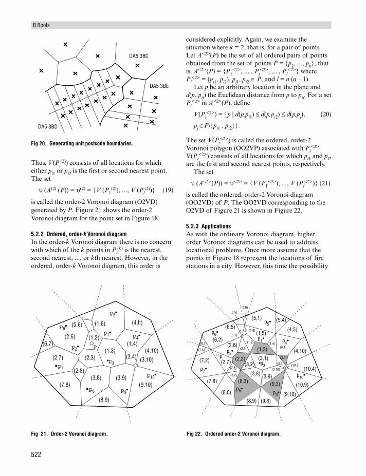
is called the order-2 Voronoi diagram (O2VD)generated by P. Figure 21 shows the order-2Voronoi diagram for the point set in Figure 18.

5.2.2 Ordered, order-k Voronoi diagram In the order-k Voronoi diagram there is no concernwith which of the k points in Pi

(k) is the nearest,second nearest, ..., or kth nearest. However, in theordered, order-k Voronoi diagram, this order is

considered explicitly. Again, we examine thesituation where k = 2, that is, for a pair of points.Let A<2>(P) be the set of all ordered pairs of pointsobtained from the set of points P = {p1, ..., pn}, thatis, A<2>(P) = {P1

<2>, ... , Pi<2>, ... , Pl

<2>} wherePi

<2> = (pi1, pi2), pi1, pi2 ∈ P, and l = n (n – 1).Let p be an arbitrary location in the plane and

d(p, pij) the Euclidean distance from p to pij. For a setPi

<2> in A<2>(P), define

V(Pi<2>) = {p | d(p,pi1) ≤ d(p,pi2) ≤ d(p,pj), (20)

pj ∈P\{pi1 , pi2}}.

The set V(Pi<2>) is called the ordered, order-2

Voronoi polygon (OO2VP) associated with Pi<2>.

V(Pi<2>) consists of all locations for which pi1 and pi2

are the first and second nearest points, respectively.The set

υ (A<2>(P)) = υ<2> = {V (P1<2>), ..., V (Pl

<2>)} (21)

is called the ordered, order-2 Voronoi diagram(OO2VD) of P. The OO2VD corresponding to theO2VD of Figure 21 is shown in Figure 22.

5.2.3 Applications As with the ordinary Voronoi diagram, higherorder Voronoi diagrams can be used to addresslocational problems. Once more assume that thepoints in Figure 18 represent the locations of firestations in a city. However, this time the possibility

B Boots

522

Fig 20. Generating unit postcode boundaries.

DA5 3BC

DA5 3BE

DA5 3BD

Fig 21. Order-2 Voronoi diagram.

(1,2)(6,7)

p6•

(2,6)

(2,7)

(7,8)

(2,8)

(2,3)

(5,6) (1,6) (4,h)

(1,4)(1,3)

•p3

(3,8) (3,9)

(8,9)

(9,10)

(3,4) (3,10)

(4,10)

•p7

•p8

p2•

p9•

p10•

p4•p1•

p5•

p

Fig 22. Ordered order-2 Voronoi diagram.

(5,6)

(6,1)

(5,1) (5,4)

(10,4)

(10,9)(8,0)

(1,5)

(6,7)

(7,6)

(2,8)

(8,2)

p6•(6,2)

(7,2)

(7,8)

(2,3)

(6,5)

(1,6) (4,5)

(1,3)

•p3

(3,8) (3,9)

(9,8)(9,10)

(10.3)

(4,10)

(9,3)

(8,9)

(8,3)

p1•

p5•

p4•

p2•

p7•

p8•p9•

p10•(3,10)

(3,4)

(3,0)(3,1)(3,2)

(2,1)

(1,2) (1,4)(4,1)

(2,7)p

(2,6)

(6,5)

is recognised that, on a given occasion, theequipment at the fire station closest to a givenlocation may already be fully committed, leading toquestions such as the following:

1 What are the two closest fire stations to a givenlocation p?

2 What are the first and the second nearest firestations to a given location p?

3 What is the region of the city for which thestation at pi is the second nearest?

Question 1 may be answered by examining theO2VD of the fire stations and observing in whichO2VP the query location p occurs. For example, thetwo nearest fire stations to p in Figure 21 are thoselocated at p1, p2. Questions 2 and 3 require theconsideration of the OO2VD of the fire stations.The answer to (2) is found by observing the OO2VPin which p is located (e.g. the first and second nearestfire stations to p in Figure 22 are those at p2 and p7,respectively). To answer question 3 we need to findall OO2VPs for which station pi is the secondnearest. The union of these polygons gives therequired region (e.g. for the station at p3 this is theshaded region in Figure 22).

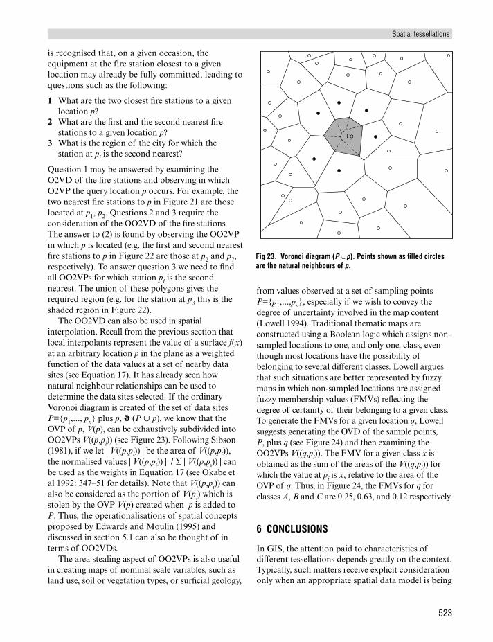
The OO2VD can also be used in spatialinterpolation. Recall from the previous section thatlocal interpolants represent the value of a surface f(x)at an arbitrary location p in the plane as a weightedfunction of the data values at a set of nearby datasites (see Equation 17). It has already seen hownatural neighbour relationships can be used todetermine the data sites selected. If the ordinaryVoronoi diagram is created of the set of data sitesP={p1,..., pn} plus p, � (P � p), we know that theOVP of p, V(p), can be exhaustively subdivided intoOO2VPs V((p,pi)) (see Figure 23). Following Sibson(1981), if we let | V((p,pi)) | be the area of V((p,pi)),the normalised values | V((p,pi)) | / ∑ | V((p,pi)) | canbe used as the weights in Equation 17 (see Okabe etal 1992: 347–51 for details). Note that V((p,pi)) canalso be considered as the portion of V(pi) which isstolen by the OVP V(p) created when p is added toP. Thus, the operationalisations of spatial conceptsproposed by Edwards and Moulin (1995) anddiscussed in section 5.1 can also be thought of interms of OO2VDs.

The area stealing aspect of OO2VPs is also usefulin creating maps of nominal scale variables, such asland use, soil or vegetation types, or surficial geology,

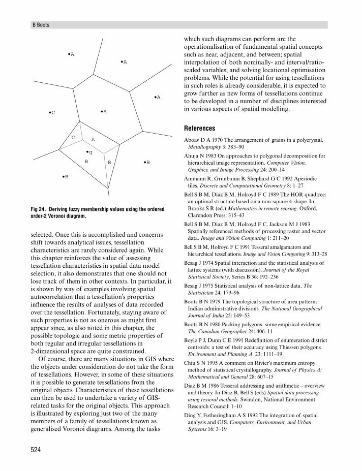
from values observed at a set of sampling pointsP={p1,...,pn}, especially if we wish to convey thedegree of uncertainty involved in the map content(Lowell 1994). Traditional thematic maps areconstructed using a Boolean logic which assigns non-sampled locations to one, and only one, class, eventhough most locations have the possibility ofbelonging to several different classes. Lowell arguesthat such situations are better represented by fuzzymaps in which non-sampled locations are assignedfuzzy membership values (FMVs) reflecting thedegree of certainty of their belonging to a given class.To generate the FMVs for a given location q, Lowellsuggests generating the OVD of the sample points,P, plus q (see Figure 24) and then examining theOO2VPs V((q,pi)). The FMV for a given class x isobtained as the sum of the areas of the V((q,pi)) forwhich the value at pi is x, relative to the area of theOVP of q. Thus, in Figure 24, the FMVs for q forclasses A, B and C are 0.25, 0.63, and 0.12 respectively.

6 CONCLUSIONS

In GIS, the attention paid to characteristics ofdifferent tessellations depends greatly on the context.Typically, such matters receive explicit considerationonly when an appropriate spatial data model is being

Spatial tessellations

523

Fig 23. Voronoi diagram (P ∪p). Points shown as filled circlesare the natural neighbours of p.

+p

selected. Once this is accomplished and concernsshift towards analytical issues, tessellationcharacteristics are rarely considered again. Whilethis chapter reinforces the value of assessingtessellation characteristics in spatial data modelselection, it also demonstrates that one should notlose track of them in other contexts. In particular, itis shown by way of examples involving spatialautocorrelation that a tessellation’s propertiesinfluence the results of analyses of data recordedover the tessellation. Fortunately, staying aware ofsuch properties is not as onerous as might firstappear since, as also noted in this chapter, thepossible topologic and some metric properties ofboth regular and irregular tessellations in2-dimensional space are quite constrained.

Of course, there are many situations in GIS wherethe objects under consideration do not take the formof tessellations. However, in some of these situationsit is possible to generate tessellations from theoriginal objects. Characteristics of these tessellationscan then be used to undertake a variety of GIS-related tasks for the original objects. This approachis illustrated by exploring just two of the manymembers of a family of tessellations known asgeneralised Voronoi diagrams. Among the tasks

which such diagrams can perform are theoperationalisation of fundamental spatial conceptssuch as near, adjacent, and between; spatialinterpolation of both nominally- and interval/ratio-scaled variables; and solving locational optimisationproblems. While the potential for using tessellationsin such roles is already considerable, it is expected togrow further as new forms of tessellations continueto be developed in a number of disciplines interestedin various aspects of spatial modelling.

References

Aboav D A 1970 The arrangement of grains in a polycrystal.Metallography 3: 383–90

Ahuja N 1983 On approaches to polygonal decomposition forhierarchical image representation. Computer Vision,Graphics, and Image Processing 24: 200–14

Ammann R, Grunbaum B, Shephard G C 1992 Aperiodictiles. Discrete and Computational Geometry 8: 1–27

Bell S B M, Diaz B M, Holroyd F C 1989 The HOR quadtree:an optimal structure based on a non-square 4-shape. InBrooks S R (ed.) Mathematics in remote sensing. Oxford,Clarendon Press: 315–43

Bell S B M, Diaz B M, Holroyd F C, Jackson M J 1983Spatially referenced methods of processing raster and vectordata. Image and Vision Computing 1: 211–20

Bell S B M, Holroyd F C 1991 Tesseral amalgamators andhierarchical tessellations. Image and Vision Computing 9: 313–28

Besag J 1974 Spatial interaction and the statistical analysis oflattice systems (with discussion). Journal of the RoyalStatistical Society, Series B 36: 192–236

Besag J 1975 Statistical analysis of non-lattice data. TheStatistician 24: 179–96

Boots B N 1979 The topological structure of area patterns:Indian administrative divisions. The National GeographicalJournal of India 25: 149–53

Boots B N 1980 Packing polygons: some empirical evidence.The Canadian Geographer 24: 406–11

Boyle P J, Dunn C E 1991 Redefinition of enumeration districtcentroids: a test of their accuracy using Thiessen polygons.Environment and Planning A 23: 1111–19

Chiu S N 1995 A comment on Rivier’s maximum entropymethod of statistical crystallography. Journal of Physics A:Mathematical and General 28: 607–15

Diaz B M 1986 Tesseral addressing and arithmetic – overviewand theory. In Diaz B, Bell S (eds) Spatial data processingusing tesseral methods. Swindon, National EnvironmentResearch Council: 1–10

Ding Y, Fotheringham A S 1992 The integration of spatialanalysis and GIS. Computers, Environment, and UrbanSystems 16: 3–19

B Boots

524

Fig 24. Deriving fuzzy membership values using the orderedorder-2 Voronoi diagram.

•A

•A

•A

•A

•B

•C

•B

B

AC

B

•q

Edwards G 1993 The Voronoi model and cultural space:applications to the social sciences and humanities. In FrankA U, Campari I (eds) Spatial information theory – atheoretical basis for GIS. Berlin, Springer: 202–14

Edwards G, Moulin B 1995 Towards the simulation of spatialmental images using the Voronoi model. ProceedingsInternational Joint Conference on Artificial Intelligence(IJCAI-95), Montreal, Canada, 19–26 August: 63–73

Fotheringham A S, Rogerson P A 1993 GIS and spatialanalytical problems. International Journal of GeographicalInformation Systems 7: 3–19

Gold C M 1990 Spatial data structures – the extension fromone to two dimensions. In Pau L F (ed.) Mapping and spatialmodelling for navigation. Berlin, Springer: 11–39

Gold C M 1991 Problems with handling spatial data – theVoronoi approach. CISM Journal 45: 65–80

Gold C M 1992 The meaning of ‘neighbour’. In Frank A U,Campari I, Formentini U (eds) Theories and methods ofspatio-temporal reasoning in geographic space. Berlin,Springer: 221–35

Goodchild M F, Haining R P, Wise S 1992 Integrating GIS andspatial data analysis: problems and possibilities. InternationalJournal of Geographical Information Systems 6: 407–23

Griffith D A 1982 Dynamic characteristics of spatialeconomic systems. Economic Geography 58: 177–96

Griffith D A 1992 What is spatial autocorrelation? Reflectionson the past 25 years of spatial statistics. L’EspaceGeographique 21: 265–80

Griffith D A 1996b Spatial autocorrelation and eigenfunctionsof the geographic weights matrix accompanying geo-referenced data. The Canadian Geographer 40: 351–67

Grunbaum B, Shephard G C 1977a Tilings by regularpolygons. Mathematics Magazine 50: 227–47

Grunbaum B, Shephard G C 1977b The 81 types of isohedraltilings in the plane. Mathematical Proceedings of theCambridge Philosophical Society 82: 177–96

Grunbaum B, Shephard G C 1986 Tilings and patterns. NewYork, W H Freeman & Co.

Haining R P, Griffith D A, Bennett R 1984 A statisticalapproach to the problem of missing spatial data using a first-order Markov model. The Professional Geographer 36: 338–45

Holroyd F, Bell S B M 1992 Raster GIS: models of rasterencoding. Computers and Geosciences 18: 419–26

Jong P de, Springer C, Veen F van 1984 On extreme values ofMoran’s I and Geary’s c. Geographical Analysis 16: 17–24

Le Caer G, Delannay R 1993 Correlations in topologicalmodels of 2D random cellular structures. Journal of PhysicsA: Mathematical and General 26: 3931–54

Lewis F T 1928 The correlation between cell division and theshapes and sizes of prismatic cells in the epidermis ofCucumis. Anatomical Record 38: 341–76

Lewis F T 1930 A volumetric study of growth and cell divisionin two types of epithelium – the logitudinally prismatic cellsof Tradescantia and the radially prismatic epidermal cells ofCucumis. Anatomical Record 47: 59–99

Lewis F T 1931 A comparison between the mosaic of polygonsin a film of artificial emulsion and in cucumber epidermis andhuman amnion. Anatomical Record 50: 235–65

Lewis F T 1943 The geometry of growth and cell division inepithelial mosaics. American Journal of Botany 30: 766–76

Lewis F T 1944 The geometry of growth and cell division incolumnar parenchyma. American Journal of Botany 31: 619–29

Loeb A L 1976 Space structures – their harmony andcounterpoint. Reading (USA), Addison-Wesley

Lowell K 1994 A fuzzy surface cartographic representation forforestry based on Voronoi diagram area stealing. CanadianJournal of Forest Research 24: 1970–80

Okabe A, Boots B, Sugihara K 1992 Spatial tessellations:concepts and applications of Voronoi diagrams. Chichester,John Wiley & Sons

Okabe A, Boots B, Sugihara K 1994 Nearest neighbourhoodoperations with generalized Voronoi diagrams. InternationalJournal of Geographical Information Systems 8: 43–71

Okabe A, Suzuki A 1995 Using Voronoi diagrams. In DresnerZ (ed.) Facility location: a survey of applications and methods.New York, Springer: 103–17

Ord J K 1975 Estimation methods for models of spatialinteraction. Journal of the American Statistical Society 70: 120–6

Perry J N 1995 Spatial analysis by distance indices. Journal ofAnimal Ecology 64: 303–14

Peshkin M A, Strandburg K J, Rivier N 1991 Entropicpredictions for cellular networks. Physical Review Letters67: 1803–6

Peuquet D J 1984 A conceptual framework and comparison ofspatial data models. Cartographica 18: 34–48

Pignol V, Delannay R, Le Caer G 1993 Characterization oftopological properties of 2-dimensional cellular structuresby image analysis. Acta Stereologica 12: 149–54

Rivier N 1985 Statistical crystallography. Structure of randomcellular networks. Philosophical Magazine B 52: 795–819

Rivier N 1986 Structure of random cellular networks. In KatoY, Takaki R, Toriwaki J (eds) Proceedings, First InternationalSymposium for Science on Form. Tokyo, KTK Scientific: 451–8

Rivier N 1990 Maximum entropy and equations of state forrandom cellular structures. In Fougere P F (ed.) Maximumentropy and Bayesian methods. Dordrecht, Clair: 297–308

Rivier N 1991 Geometry of random packings and froths. InBideau D, Dodds J A (eds) Physics of granular media. NewYork, Nova Science: 3–25

Rivier N 1993 Order and disorder in packings and froths. InBideau D, Hansen A (eds) Disorder and granular media.Amsterdam, Elsevier Science: 55–102

Spatial tessellations

525

Rivier N 1994 Maximum entropy for random cellular structures.In Nadal J P, Grassberger P (eds) From statistical mechanics tostatistical inference and back. Dordrecht, Clair: 77–93

Rivier N, Lissowski A 1982 On the correlation between sizesand shapes of cells in epithelial mosaics. Journal of PhysicsA: Mathematical and General 15: L143–8

Sambridge M, Braun J, McQueen H 1995 Geophysicalparameterization and interpolation of irregular data usingnatural neighbours. Geophysical Journal International 122:837–57

Samet H 1989 The design and analysis of spatial datastructures. Reading (USA), Addison-Wesley

Sibson R 1981 A brief description of natural neighbourinterpolation. In Barnett V (ed.) Interpreting multivariatedata. New York, John Wiley & Sons Inc. 21–36

Watson D F 1992 Contouring: a guide to the analysis anddisplay of spatial data. Oxford, Pergamon Press

Watson D F, Philip G M 1987 Neighbourhood-basedinterpolation. Geobyte 2: 12–16

Zaninetti L 1993 Dynamical Voronoi tessellation IV. Thedistribution of the asteroids. Astronomy and Astrophysics276: 255–60

B Boots

526