362784: Self-Associating Systems in the Analytical Ultracentrifuge

Self-Associating Systemsin the Analytical Ultracentrifuge

Donald K. McRoriePaul J. Voelker

Research and Applications DepartmentSpinco Business Unit

Beckman Instruments, Inc.Palo Alto, California

ii

Front CoverThe computer-generated graphic of a cytochrome c dimer was pro-

vided courtesy of Don Gregory, Molecular Simulations, Inc., Burlington,Massachusetts.

iii

Contents

Glossary ................................................................................................ vi

Introduction ............................................................................................1

Molecular Weight Determination by Sedimentation Equilibrium .......3

Initial Experimental Approach to AnalyzingSelf-Associating Systems ...............................................................7

Molecular Weight vs. Concentration Diagnostic Graphs ......................9

Nonlinear Least-Squares Analysis ...................................................... 13Least-Squares Methods .................................................................13Mathematical Models ....................................................................15

Single ideal species ................................................................15Self-association ......................................................................16Nonideality .............................................................................21Fitting data to a model ...........................................................21Confidence intervals ..............................................................22Contour maps .........................................................................22

Goodness of Fit ................................................................................... 24Residuals .......................................................................................24Chi Square .....................................................................................26Parameter Correlation ...................................................................26

Summary ............................................................................................. 27

Appendix A: A Rational Approach to Modeling Self-AssociatingSystems in the Analytical Ultracentrifuge .................................. 28

1. What Questions Need To Be Answered?...............................282. Don’t Vary Everything At Once ............................................283. Determine M and n ................................................................294. Baseline Considerations .........................................................305. Single Data Files, Then Multiple Data Files ..........................316. Start with the Simple Model First ..........................................327. Model in Steps .......................................................................328. Check for Physical Reality ....................................................339. Problems in Fitting .................................................................33

10. Model to Synthetic Data ........................................................34

iv

11. The Model as a Diagnostic Tool ............................................34Optimum Diagnostic Conditions: ..........................................351. Evaluating an ideal associating system. ..........................352. Evaluating a heterogeneous noninteracting system. .......353. Evaluating for nonideality. ..............................................35Realistic Diagnostic Conditions: ...........................................361. Association and nonideality in the same system. ...........362. Association and heterogeneity in the same system. ........36

12. Test the Fit and the Model .....................................................3713. Flow Chart .............................................................................3714. Limitations .............................................................................37

Appendix B: Partial Specific Volume ................................................ 40

Appendix C: Solvent Density ............................................................. 47

References ........................................................................................... 51

v

FiguresFigure 1 Graph of ln(c) vs. r2 showing curves from ideality .................4Figure 2 Molecular weight averages ......................................................5Figure 3 Optimum speeds for equilibrium runs if either molecular

weight or sedimentation coefficient can be estimated .............8Figure 4 Diagnostics graph providing a qualitative characterization of

the solution behavior of macromolecules ................................9Figure 5 Multiple data sets graphed in terms of molecular weight

vs. concentration ....................................................................10Figure 6 Diagnostics graph providing a qualitative characterization

of the solution behavior of macromolecules ..........................11Figure 7 Error surface graphs showing the sum of squares graphed

on z-axis .................................................................................14Figure 8 Concentration distributions of equilibrium in the analytical

ultracentrifuge for a monomer-tetramer model ......................17Figure 9 Actual contour maps in relation to linear approximations .....23Figure 10 Residuals from desired fit ......................................................25Figure 11 A simulated monomer-dimer association ..............................30

TablesTable 1 Amino Acids at 25°C .............................................................42Table 2 Carbohydrates at 20°C ...........................................................43Table 3 Denaturants at 20°C ...............................................................44Table 4 Miscellaneous at 20°C ...........................................................45Table 5 φ for Proteins in 6 M Guanidine-HCl and 8 M Urea .............46Table 6 Coefficients for the Power Series Approximation of

the Density .............................................................................48

vi

Glossary

A AbsorbanceB Second virial coefficientc Solute concentration (g/L)cr Solute concentration at radial distance rcro

Concentration of the monomer at the reference radius r0E Baseline offsetG Gibbs free energyH EnthalpyKa Association equilibrium constantM Monomer molecular weightMn, Mw, Mz Number-, weight- and z-average molecular weightsMw,app Apparent weight-average molecular weightR Gas constant (8.314 J mol-1 K-1)r Radial distance from center of rotationr0 Reference radial distanceS EntropyT Temperature in Kelvinv Partial specific volumeρ Solvent densityφ Isopotential partial specific volumeΣ Summation symbolχ2 Goodness of fit statisticω Angular velocity (radians/second)

1

Introduction

Studying associating systems in the analytical ultracentrifuge allows one tofully characterize the thermodynamics of these association reactions atequilibrium. An advantage to the experimenter is that the macromoleculecan be studied directly in solution under conditions of choice. By varyingthese conditions, several parameters can be determined: molecular weights,stoichiometry, association constants (tightness of binding), nonidealitycoefficients, and thermodynamic parameters such as the changes in Gibbsfree energy, enthalpy, and entropy associated with binding (∆G, ∆H, and∆S). These parameters can be studied with both self-associating systemsand associations of unlike species (hetero-associations). This primer willdescribe both simple and complex methods needed to examine self-associ-ating systems in an approach requiring little or no advance knowledge ofthe characteristics of the interactions involved. Hetero-associations requirea different approach and will be covered in a separate review.

The initial characterization of an association reaction involves severalexperiments to obtain information about the homogeneity of the system,monomer molecular weight, reversibility of the reaction, stoichiometry,and nonideality. These experiments require various run conditions and theuse of data analysis procedures and diagnostic plots that provide estimatesfor these characteristics. The most straightforward initial approach is tomeasure molecular weights under denaturing vs. native conditions. Asimple average molecular weight determination will reveal if an associa-tion is taking place and provide an initial estimate of stoichiometry. Furtherdiagnostic plots may give better estimates of stoichiometry, reversibility,and nonideality.

When initial experiments yield sufficient information, more detailedanalysis can be undertaken. Through the use of nonlinear regression tech-niques, a more accurate analysis of the system is accomplished by directfitting of the primary data to a model describing the association. By com-paring goodness of fit of the experimental data to the calculated data, amodel best describing the association can usually be discerned. Care mustbe taken in statistical analysis to ensure that the fit of the data to the se-lected model is significantly better than to alternative models. If not, moreexperiments may be needed to distinguish between models. Fitting in thismanner can give accurate determination of average molecular weights,(Mn, Mw, and Mz), association constants, and nonideality as measured byvirial coefficients. Also, this procedure allows one to confirm stoichiom-

2

etries estimated from other experiments and to incorporate baseline errorsin the data.

In all calculations, several parameters are needed: ω2, determined fromthe rotor speed; R, the gas constant; T, the temperature in Kelvin; v, thepartial specific volume determined from the sample composition or bymeasurement, and ρ, the density determined from the solvent composition.The last two are the most variable in a system and can therefore lead to thegreatest error in calculations.

From a single experiment, only the buoyant molecular weight is mea-surable directly in the analytical ultracentrifuge. This value, M(1 - vρ), isthe molecular weight of the sample corrected by a buoyancy factor due todisplaced solvent. In the case of multiple species, M(1 - vρ) will be a statis-tical average of the molecular weights of all species present in solution.Different molecular weight averages can be determined by various treat-ments of sedimentation equilibrium data. More detailed analyses of theassociations as described above require that the data from several experi-ments be examined simultaneously.

Three parameters necessary for the analysis of self-associating systemsare not determined by run conditions. These are v, ρ, and monomer mo-lecular weight. Calculation of these parameters is needed to begin ananalysis. Calculations of v and ρ are described in Appendixes B and C,respectively. If sample composition is not known, monomer molecularweight can be determined experimentally from a run in denaturing condi-tions. Also, alternative methods such as mass spectrometry give accuratesubunit molecular weight determinations.

3

Molecular Weight Determinationby Sedimentation Equilibrium

When sedimentation and diffusion come to a state of equilibrium, no ap-parent movement of solute occurs. The equilibrium concentration distribu-tion is dependent on the buoyant molecular weight, M(1 - vρ); angularvelocity, ω2; and temperature. Since the concentration distribution is de-pendent on the buoyant molecular weight, it is obvious that accurate valuesof v and ρ are necessary for the determination of molecular weight fromequilibrium conditions.

From the Lamm (1929) equation describing movement of molecules ina centrifugal field, the following equation can be derived for a single, ther-modynamically ideal solute:

ln(cr )

r2 = M(1 − vρ)ω2

2RTEquation 1

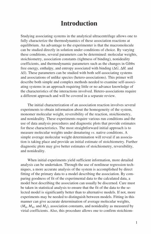
A plot of ln(c) vs. r2 will yield a straight line with a slope proportionalto M. For nonideal or associating systems, or when multiple species arepresent, a straight line is not obtained, and more rigorous analysis isneeded. Nevertheless, as shown in Figure 1, this analysis provides a firstapproximation of M and can indicate thermodynamic nonideality or poly-dispersity in the sample.

4

ba

c

r2

ln (c)

Figure 1. Graph of ln(c) vs. r2 showing curves from ideality

From the graph it is apparent that nonideality and polydispersity haveopposite effects so that the presence of both in a sample may be offsettingand thus not discernible. It should also be noted that small amounts ofaggregation, such as 10% or less of a sample present as a dimer, will not bedetectable by this method.

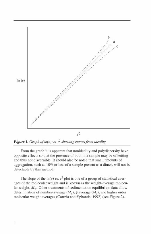
The slope of the ln(c) vs. r2 plot is one of a group of statistical aver-ages of the molecular weight and is known as the weight-average molecu-lar weight, Mw. Other treatments of sedimentation equilibrium data allowdetermination of number-average (Mn), z-average (Mz), and higher ordermolecular weight averages (Correia and Yphantis, 1992) (see Figure 2).

5

Mn =

Mw =

Mz =

(number-average)

(weight-average)

(z-average)

∑niMi

∑ni

∑niMi2

∑niMi

∑niMi3

∑niMi2

∑ci

∑ci/Mi

∑ciMi

∑ci

∑ciMi2

∑ciMi

=

=

=

i i

i i

i i

i i

i i

i i

Concentrationof

Molecules(ci)

Molecular Weight ( Mi )

Mn

Mw

Mz

Figure 2. Molecular weight averages. a) Calculation of molecular weightaverages; b) graph showing distribution in a polydisperse system.

If the solution is polydisperse, then sedimentation equilibrium experi-ments yield an average molecular weight, not that of any single compo-nent. Mn , Mw, and Mz give increasing significance, respectively, to thosecomponents in a mixture with the highest molecular weights. Thus, for apolydisperse system, Mn < Mw < Mz. If a solution is monodisperse, thenMn = Mw = Mz. A comparison of the molecular weight averages can there-fore provide a good measure of homogeneity.

If the plot of ln(c) vs. r2 is nonlinear, tangents to the curve yield aweight-average molecular weight for the mixture of species present at each

(a)

(b)

6

radial position. In this manner the user can obtain molecular weight as afunction of increasing solute concentration moving down the cell. Overlay-ing plots of data from samples of different starting concentrations willprovide information about the presence of more than one species in thecell, the ability to distinguish polydisperse and self-associating systems,and, in the latter case, an estimate of the monomer molecular weight andstoichiometry.

7

Initial Experimental Approach toAnalyzing Self-Associating Systems

An initial level of analysis involves a characterization of the sample usingdiagnostic graphs. This level of analysis is qualitative and simply deter-mines if the sample is homogeneous, ideal, and whether or not a self-asso-ciation is occurring. In many cases, estimates of monomer molecularweight and stoichiometry are also possible at this level, but quantitativedetermination of thermodynamic parameters will require more rigorousnonlinear least-squares fitting procedures that will be described in moredetail in a following section. Qualitative analyses do, however, provideexcellent starting guesses for models in more complex analyses.

To determine these parameters, data from runs under both denaturingand nondenaturing conditions need to be compared. The two most com-monly used denaturants are 8 M urea and 6 M guanidine-HCl. Both haveeffects on v which should be taken into account during data analysis. Inaddition, data from samples run at multiple starting concentrations andmultiple rotor speeds will be required. This approach is described by Laue(1992).

Typically, a range of starting concentrations with absorbances from0.1 to 1.0 is employed. The simplest way to obtain this range of concentra-tions is to perform a serial dilution. Generally, the absorbance variation isscaled for a single wavelength, but if the extinction coefficients are knownfor several wavelengths, this added information can be used to convert allabsorbances to the same concentration scale using the Beer-Lambert Law,*

which permits an even wider range of concentrations to be used.

Rotor speeds are chosen to straddle the estimated optimum rotor speedfor the sedimentation equilibrium run. Figure 3 shows optimum speeds foran equilibrium run if either the molecular weight or sedimentation coeffi-cient can be estimated for the sample.

* Beer-Lambert Law: A = log(I0/I) = εcl, where I0 = intensity of the inci-dent radiation; I is the intensity of light transmitted through a pathlength lin cm, containing a solution of concentration c moles per liter; ε is themolar extinction coefficient with units liter mole-1 cm-1; A is the absor-bance.

8

0.25 1 2 3 4 5 6 10 20 30

100

10

1.0

1.0 10 100 1000

Molecular Weight in Thousands

rpm

in T

hous

ands

Approximate Sedimentation Coefficient

Figure 3. Optimum speeds for equilibrium runs if either molecular weightor sedimentation coefficient can be estimated. (Reprinted from Chervenka,1970.)

A set of at least three speeds is chosen to yield significantly varieddata for the diagnostics (Laue, 1992). For three speeds, the ratio of thesquares of the two slower speeds should be 1.4 or greater, and the ratio ofthe squares of the fastest and slowest speeds should be 3 or greater. Forexample, if an optimum rotor speed is estimated as 20,000 rpm, a goodchoice of three speeds would be 16,000, 20,000, and 30,000 rpm[(20,000/16,000)2 = 1.56 and (30,000/16,000)2 = 3.52]. Data should beacquired at the lowest speed first, then at progressively higher speeds tominimize the time to reach equilibrium. If data need to be acquired at aslower speed, it is advantageous to stop the rotor and gently shake the cellsrather than simply lowering the speed, because redistribution from diffu-sion is quite slow.

9

Molecular Weight vs. ConcentrationDiagnostic Graphs

The data collected as described in the preceding section allow the apparentmolecular weight to be plotted as a function of sample loading concentra-tion and rotor speed. Since the sample was run under denaturing condi-tions, Mw can also be calculated relative to monomer molecular weight.These graphs provide an initial characterization of the system with respectto: 1) homogeneity, 2) nonideality, 3) self-association (with limited infor-mation about stoichiometry), and 4) polydispersity.

Laue (1992) uses a plot of the apparent weight-average molecularweight vs. the midpoint absorbance (Figure 4). If the sample obeys theBeer-Lambert Law, absorbance and concentration will be proportional.

2.00

1.50

1.00

0.50

0.000.00 0.70 1.40 2.10 2.80

Link Protein

Myo D

DSPG GAG

Concentration (mg/mL)

Mw

,app

/M

Figure 4. Diagnostics graph providing a qualitative characterization of thesolution behavior of macromolecules. (Reprinted from Laue, 1992.)

This graph is useful in the detection of three possible conditions in thesample run with multiple concentrations. If the molecular weight remainsconstant with changing absorbance (concentration), a single ideal species isindicated. If the molecular weight decreases with increasing absorbance,this indicates thermodynamic nonideality. Finally, if the molecular weightincreases with increasing concentration, a self-association may be occur-ring. In this last case, if a wide enough concentration range is examined,the molecular weight at low concentration will approach that of the small-

10

est species in the reaction, and at higher concentrations it will approachthat of the largest species. If the monomer molecular weight has been de-termined under denaturing conditions, this provides estimates of the stoi-chiometry of these limiting species. As is the case for plots of ln(A) vs. r2,association and nonideality have opposing effects. So, if both conditionsare present, determination of an upper limit for oligomerization is difficult.Similar problems may arise due to limited solubilities at higher concentra-tions.

More information can be obtained from plots of molecular weight vs.concentration from a single sample by examining the apparent weight-average molecular weight as a function of increasing radius. One method isto use nonlinear regression techniques to calculate parameters that allowdetermination of molecular weight for each radial position in the cell, thento graph the molecular weight vs. the corresponding absorbance value(Formisano et al., 1978). Another method is to take subsets of the data,determine molecular weight from linear regression analysis with a plot ofln(A) vs. r2, and finally graph the molecular weight against the midpointabsorbance of the subset. Other methods are used in some cases to avoidthe systematic errors that occur in some calculations (Dierckx, 1975).Mw vs. concentration calculations provide information similar to that ob-tained from a single point per sample, but, in addition, a diagnostic graphthat distinguishes between self-association and polydispersity may be ob-tained (Figure 5).

cr

Mw

cr

Mw

Figure 5. Multiple data sets graphed in terms of molecular weight vs. con-centration. a) Self-associating system; b) polydisperse system.

For a self-associating system, the apparent weight-average molecularweight will increase with increasing concentration, and the plots of Mw vs.absorbance will coincide. As with the previous diagnostic graphs, the limit-ing molecular weights will approach that of the monomer at the lower

(a) (b)

11

concentrations and that of the largest species at the higher concentrations.Nonideality will cause a downward trend in the slope and will prevent anaccurate estimation of the stoichiometry from this plot.

In the case of polydispersity, however, the Mw vs. absorbance plotswill not coincide but will be displaced to the right with increasing samplestarting concentration. Nonoverlapping weight-average molecular weightdistributions will be observed for different loading concentrations. Thisobservation is due to the fact that the same molecular weight distribution ispresent regardless of sample concentration.

Polydispersity and reversibility of a self-association reaction can beconfirmed by graphs of apparent molecular weight as a function of rotorspeed (Figure 6).

1.20

0.90

0.60

0.30

0.001.00 1.25 1.50 1.75 2.00

DSPGI Core

LexA

rpm/rpm0

Mw

,app

/M

Figure 6. Diagnostics graph providing a qualitative characterization of thesolution behavior of macromolecules. (Reprinted from Laue, 1992.)

For both homogeneous, noninteracting samples and homogeneous,self-associating samples, molecular weight is independent of rotor speed aslong as all associating species are detectable in the concentration gradient.Polydisperse samples, however, display a systematic decrease in molecularweight with increasing rotor speed.

Caution is required due to the opposing effects of association andnonideality on concentration dependence of molecular weight. The pres-ence of both phenomena can produce apparently ideal behavior. The effectof nonideality may not be apparent except in higher concentrations. In this

12

case, the molecular weight will appear to decrease with increasing concen-tration. This situation makes estimation of association stoichiometry diffi-cult. These diagnostic plots should only be considered qualitative and notused for numeric determination of any molecular weight, association, ornonideality parameters.

13

Nonlinear Least-Squares Analysis

Least-squares methods are one way to obtain a statistical fit of the experi-mental data to a proposed model and to obtain best estimates for unknownparameters (Johnson, 1992; Johnson and Faunt, 1992; Johnson and Frazier,1985; Johnson et al., 1981). The major advantage of these methods is thatdata can be analyzed directly without transformation. Also, more complexmodels can be tested when obvious differences between experimental andfitted data exist. Computer analysis has greatly facilitated these methods.Without the calculating power of the computer, only the conventionalgraphical analyses with their inherent assumptions and approximationswould be possible. Three basic features are needed for simple nonlinearleast-squares analysis: 1) an algorithm for calculating least-squares, 2) amathematical model to describe the system, and 3) statistical analysis tomeasure goodness of fit of a proposed fitted model to the experimentaldata. A practical approach to data analysis using these methods and theBeckman Optima™ XL-A Data Analysis Package is described in Appen-dix A.

Least-Squares Methods

In this analysis, a series of curves is calculated to locate a “best” fittingmodel of the data. Each iteration leads to a better approximation of thecurve parameters until the approximations converge to stable values for theparameters being varied. For least-squares analysis, the differences be-tween the fitted function and the experimental data are squared andsummed, and the parameters varied so as to minimize this sum. Ideally, thereduction continues until a global minimum is reached. Minimization ofleast-squares does not always provide the correct set of model parameters.Therefore, additional statistical and graphical analysis is usually needed inaddition to curve fitting techniques.

The graphs in Figure 7 show the sum of squares minima in relation totwo parameters.

14

Figure 7. Error surface graphs showing the sum of squares graphed onz-axis. Two variables are shown on the x- and y-axes. a) Well-defined mini-mum; b) well-defined for y but not x.

The values for the two parameters are on the x- and y-axis, respectively,and for the sum of squares on the z-axis. In Figure 7a the error space iswell defined for both parameters, and the algorithm would be able to calcu-late them to a high precision. Figure 7b, however, shows an example wherethe parameter plotted on the y-axis is well defined, but the parameter plot-ted on the x-axis is not. In this case, the algorithm would be able to calcu-late the y parameter to a high precision, but would have more difficultycalculating the x parameter to the same precision. In some cases, the errorspace can be flat or contain several minima that may yield different an-swers depending on starting guesses.

Many numerical algorithms are available for determining parametersby least-squares and are too numerous to be listed here. The Marquardtmethod (1963) is the most commonly used. It combines the advantages oftwo other methods, Gauss-Newton and Steepest Descent (Bevington,1992), to obtain a more robust convergence. The Nelder-Mead algorithm(1965), also known as the Simplex method, is a geometric, rather than anumeric, procedure. The XL-A Data Analysis Package has incorporated amodification of the Gauss-Newton method developed by Johnson et al.(1981) in the multifit program analyzing multiple data sets simultaneously.Also accessible is the Marquardt algorithm for single data file analysis.

(b)(a)

15

Mathematical Models

Single ideal species

When a method of least-squares analysis is used, a mathematical equation,or model, describing the distribution of the macrosolute in the cell isneeded for the fitting procedure. The initial model chosen can be one thatseems best to describe the system as discerned from the diagnostic plotsdescribed earlier. From goodness of fit analyses, alternative models arethen analyzed to find the best description of the experimental data.

As described previously, the Lamm partial differential equation de-scribes all movement of molecules in a centrifugal field. At equilibrium, noapparent movement of solute occurs due to the equalization of sedimenta-tion and diffusion. From this observation, an exponential solution to theLamm equation can be derived (Equation 2). This equation, with cr andradius as the dependent and independent variables, respectively, is directlyrelated to the data as it is obtained from the analytical ultracentrifuge.

cr = cr0e[ ω2

2RTM(1−vρ)(r2 − r0

2 )]Equation 2

where cr = concentration at radius rcr0

= concentration of the monomer at the reference radius r0ω = angular velocityR = gas constant (8.314 × 107 erg/mol⋅K)T = temperature in KelvinM = monomer molecular weightv = partial specific volume of the soluteρ = density of solvent

Ultracentrifuge data can be fitted to this equation using optical absor-bance in place of concentration, provided the sample obeys the Beer-Lam-bert Law across the full range of absorbance. Final results are usually con-verted back to concentration.

Equation 2 describes distribution of a single ideal species at equilib-rium. Fitting the data to this model using nonlinear regression analysisyields an apparent weight-average molecular weight for all solutes in thecell when the baseline offset is constrained to zero. Including the baselineoffset will result in determination of a z-average molecular weight. Recall-

16

ing from Figure 2 that these average molecular weights are expressed interms of concentration, the molecular weights are not well defined aver-ages if the extinction coefficients are not known for all components be-cause the data used are absorbance values.

Baseline offset results from a difference in the absorbance between thereference and the solvent in which the sample is dissolved. Usually, exten-sive dialysis procedures are used to minimize the difference. If, however, adifference remains, the baseline term must be included in the mathematicalmodel. With sufficient data, the baseline can be varied as an additionalparameter, but the calculated values of other parameters such as molecularweight are affected greatly by the baseline value. The baseline value can bedetermined experimentally by a high-speed run where the meniscus isdepleted of all sample and the absorbance read directly from the data nearthe meniscus. The experimental approach is limiting when the meniscuscannot be depleted.

Self-association

The model equation for a self-associating system is similar to that of asingle ideal species except that the total absorbance at a given radius is thesum of absorbances of all species at that radius. Each term of the summa-tion will be a distribution function similar to that for a single ideal species.Take, for example, the simple equilibrium:

monomer ↔ n-mer

At equilibrium, the total absorbance as measured in the analyticalultracentrifuge can be shown as the sum of two species (Figure 8).

17

Mac

roso

lute

Con

cent

ratio

n

Radial Distance

10,000 rpm

totalm

acro

solu

teco

ncen

tratio

n

M = 45,000 g/mol speciesM

=18

0,00

0g/

mol

spec

ies

6.70 cm 7.00 cm

Figure 8. Concentration distributions of equilibrium in the analyticalultracentrifuge for a monomer-tetramer model showing monomer (----),tetramer (- - -), and total concentrations ( ).

18

The equation that describes the total macrosolute distribution for thismonomer–n-mer equilibrium is as follows:

ctotal = cmonomer, r0e[ ω2

2RTM(1−v ρ)(r2 − r0

2 )]

+ cn−mer,r0e[ ω2

2RTnM(1−v ρ)(r2 − r0

2 )] Equation 3

Each exponential in the summation describes the equilibrium distribu-tion of an individual species in the equilibrium, the first being the mono-mer and the second the n-mer. The stoichiometry is set in the model by aninteger value for n, such that the n-mer molecular weight is n times themonomer molecular weight, M.

For the monomer–n-mer equilibrium reaction, the association constantis:

Ka = cn-mer/(cmonomer)n Equation 4

Substituting into equation 3, gives a new model to solve directly for Kawithout the cn-mer term:

ctotal = cmonomer,r0e[ ω2

2RTM(1−v ρ)(r2 − r0

2 )]

+ Ka (cmonomer,r0)n e[ ω2

2RTnM(1−v ρ)(r2 − r0

2 )] Equation 5

Rearranging the equation constrains the cmonomer,r0 and Ka terms to

positive numbers:

ctotal,r = e[ln(cmonomer ,r0

)+ ω 2

2RTM(1−v ρ)(r 2 − r 0

2 )]

+ e{n[ln(cmonomer ,r0

)]+ ln(K a )+ ω 2

2RTnM(1−v ρ)(r 2 − r 0

2 )} Equation 6

19

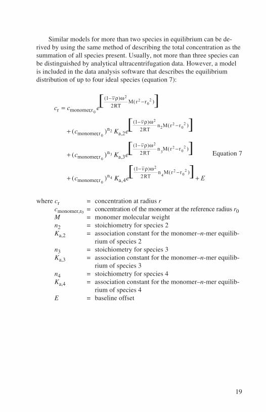
Similar models for more than two species in equilibrium can be de-rived by using the same method of describing the total concentration as thesummation of all species present. Usually, not more than three species canbe distinguished by analytical ultracentrifugation data. However, a modelis included in the data analysis software that describes the equilibriumdistribution of up to four ideal species (equation 7):

cr = cmonomer,r0e[(1−v ρ)ω2

2RTM(r2 − r0

2 )]

+ (cmonomer,r0)n2 Ka,2e[

(1−v ρ)ω2

2RTn2M(r2 − r0

2 )]


(1−v ρ)ω2

2RTn 3M(r2 − r0

2 )]


(1−v ρ)ω2

2RTn 4M(r2 − r0

2 )]+ E

Equation 7

where cr = concentration at radius rcmonomer,r0

= concentration of the monomer at the reference radius r0M = monomer molecular weightn2 = stoichiometry for species 2Ka,2 = association constant for the monomer–n-mer equilib-

rium of species 2n3 = stoichiometry for species 3Ka,3 = association constant for the monomer–n-mer equilib-

rium of species 3n4 = stoichiometry for species 4Ka,4 = association constant for the monomer–n-mer equilib-

rium of species 4E = baseline offset

20

Rearranging as before to constrain cmonomer,r0 and Ka values:

cr = e[ln(cmonomer, r0

)+ (1−vρ)ω2

2RTM(r2 −r0

2 )]

+ e{n2[ln(cmonomer, r0

)]+ln(Ka,2 )+ (1−vρ)ω2

2RTn2M(r2 −r0

2 )}


)]+ln(Ka,2 )+ (1−vρ)ω2

2RTn3M(r2 −r0

2 )}


)]+ln(Ka,2 )+ (1−vρ)ω2

2RTn4M(r2 −r0

2 )}+ E

Equation 8

The stoichiometries n2-n4 are defined by the user, and the respectiveassociation constants are for the monomer–n-mer equilibrium of each ag-gregate. Association constants for n-mer–n-mer equilibria can be calcu-lated from respective monomer–n-mer constants, but these mechanisms ofreaction cannot be confirmed from equilibrium concentration data. Forexample, with a monomer-dimer-trimer equilibrium, the model (equation8) will calculate the association constants for the monomer-dimer andmonomer-trimer equilibria. If there is evidence that a dimer-trimer equilib-rium is present, it can be calculated:

K1-2 = cdimer/(cmonomer)2, K1-3 = ctrimer/(cmonomer)

3 Equation 9a

so K2-3 = ctrimer/cmonomer • cdimer = K1-3/K1-2 Equation 9b

Usually, association constants are expressed in terms of concentration.Since data from the analytical ultracentrifuge are in absorbance units, someassumptions are usually made in the calculation of these constants. Theextinction coefficient for an n-mer in the monomer–n-mer equilibrium isassumed to be n times that of the monomer. So, if an association constantis calculated in terms of the absorbance data, conversion to one based onconcentration must include this assumption (Becerra et al., 1991; Rosset al., 1991). Equation 10 shows this conversion if the extinction coeffi-cient of the monomer is known:

K1-2,conc = c2/c12 = K1-2,absεl/2;

Beer-Lambert Law: A = εcl or c = A/εl Equation 10

21

Similarly, for a monomer-trimer system the conversion is:

K1-3,conc = c3/c13 = K1-3,absε2l2/3 Equation 11

Nonideality

Nonideal behavior of an associating system resulting from charge orcrowding can be incorporated into the model (equation 12). The nonideal-ity is described by the second virial coefficient, B (Haschmeyer and Bow-ers, 1970; Holladay and Sophianopolis, 1972, 1974).

cr,total = e[ln(cmonomer,r0

)+ (1−vρ)ω2

2RTM(r2 − r 0

2 )−BM(ctotal,r −ctotal,r0)]

+e[ln(cmonomer,r0

)+ ln(Ka,2 )+ (1−vρ)ω2

2RTn2M(r2 − r0


+e[ln(cmonomer,r0

)+ ln(Ka, 3)+ (1−vρ)ω2

2RTn3M(r2 − r0


+e[ln(cmonomer,r0

)+ ln(Ka,4)+ (1−vρ)ω2

2RTn4M(r2 − r0


+ E

Equation 12

This model can also be used for fitting all previously described equi-libria with appropriate constraints. For example, setting the virial coeffi-cient value to zero effectively removes all nonideality terms, and the modelis the same as that described for an ideal self-associating system. Also,constraining any of the association constant values to an extremely smallnumber, e.g., 1 × 10-20, effectively removes the exponent term describingthe distribution of the corresponding n-mer. This constraint can make thesame model usable for one to four species in the cell.

Fitting data to a model

Once a model has been chosen along with the algorithm for analysis, theuser is ready to begin the fitting procedure. The basis for fitting is to setinitial guesses for all parameters in the model and either to constrain theseto the set value or to allow them to float in the least-squares calculation.The constrain/vary choice will be dictated by experimental conditions andthe thermodynamic parameters to be determined. Certain parameters aredetermined by experimental conditions and must be provided prior to thefitting procedure. These include angular velocity (ω2) determined from therotor speed, temperature, and characteristics of the solute and solvent

22

( v and ρ). A reference radius will also be chosen for the fitting procedure.In all cases, the absorbance or concentration at this reference radius will beallowed to float in the calculations. All other parameters are chosen by theuser.

The amount of data will be the factor limiting the complexity of themodels that can be distinguished statistically. For example, with a singledata set, floating variables should be limited to two. Even then, confidencein answers obtained is not always good enough. So, as a general rule, mul-tiple data sets with varying conditions (usually speed and starting sampleconcentration) should be used. In this case, an algorithm is needed that canfit to the multiple data sets simultaneously.

Analysis of multiple files separately can also be used to check thereversibility of an associating system. If the same association constant isobtained from runs at multiple speeds and starting concentrations, the asso-ciation is reversible.

Confidence intervals

Confidence intervals are a measure of the precision of individual param-eters based on a single set of data. However, the interval determined for aparameter can also serve as a measure of the accuracy of the estimatedparameter (Johnson and Faunt, 1992). A number of methods of varyingcomplexity exist to evaluate confidence intervals and, thus, the validity ofthe approximation (Johnson and Faunt, 1992; Straume and Johnson,1992b). Confidence intervals in most cases are not symmetrical, so themagnitudes of the two intervals from a determined parameter are not al-ways equivalent. This asymmetry makes these intervals more realistic thansymmetrical standard deviation determinations or linear approximations ofconfidence intervals that are symmetrical around the determined parameter.

Contour maps

Contours are a method of profiling a three-dimensional surface in a two-dimensional format. In this way, the user can visualize the sum of squareserror space in relation to two parameters (Bates and Watts, 1988; Johnsonand Faunt, 1992). Using the error surface maps illustrated in the least-squares section, one can calculate confidence intervals corresponding tothe magnitude of the sum of squares on the z-axis. Planes drawn parallel tothe x-y axes at increasing magnitudes along the z-axis will intersect theerror surface. When viewed down the z-axis, the intercepts will appear as

23

concentric contours. The contours will show graphically the magnitude ofthe confidence intervals on the x- and y-axes in relation to the minimum ofthe sum of squares.

Several methods exist for estimating the contours. The actual contoursfor nonlinear regression are asymmetrical, but to save computer time, inmany cases, linear or symmetric approximations are used to calculate ellip-tical estimations (Figure 9).

Figure 9. Actual contour maps ( ) in relation to linear approximations(- - -) to demonstrate differences in confidence intervals; + represents theleast-squares estimate. (Redrawn from Bates and Watts, 1988, with permis-sion of John Wiley & Sons, Inc.)

The spacing and shape of the contours can indicate how well the twoparameters being examined are defined by the error space. Closer and lesselongated (rounder) contours indicate better defined parameters.

24

Goodness of Fit

The first fitting attempt for any experiment is usually to the single idealspecies model. The Mw and Mz determined will give the first indication ofpossible inappropriateness of the model for the experimental data. If thesemolecular weight averages are not equivalent, multiple species are indi-cated. If a monomer molecular weight is known from previous experi-ments, Mw will provide the first indication of the stoichiometry of an asso-ciating system. But, as mentioned previously, nonideality will haveopposite effects on the analysis, and this fact should be considered in inter-pretation of results.

Residuals

The most sensitive graphical representation for goodness of fit, and thebest indicator of possible alternative models, is the residual plot. Residualsare the difference between each experimental data point and the corre-sponding point on the curve calculated from the model equation. Figure 10shows an example of the desired residuals with a fit from a plausiblemodel.

A random distribution of points about the zero value is a desired diag-nostic for a good fit. Also shown are typical patterns of systematic errorscharacteristic of associating and nonideal systems. Thus, the patterns ofresidual plots can suggest additional models for fitting.

25

0.02

0.00

-0.027.0 7.2

Radius (cm)

Res

idua

ls

(a)

0.15

6.80

Radius (cm)

Res

idua

ls

0.20

0.10

0.05

0.00

-0.05

-0.106.85 6.90 6.95 7.00 7.05 7.10 7.15

(b)

Radius (cm)

Res

idua

ls

0.02

0.01

0.00

-0.01

-0.026.90 7.057.00 7.207.10 7.156.95

(c)

Figure 10. Residuals from desired fit. a) Good fit; b) aggregation;c) nonideality.

26

Chi Square

Several mathematical analyses are used for determining goodness of fit(Straume and Johnson, 1992a). Of these, the χ2 test is probably the mostcommon. Once it is clear that there are no systematic trends in the residualplot, the χ2 test provides a quantitative measure for the goodness of fit of aparticular model. The χ2 statistic is defined as:

χ2 =(observed residual - expected residual)i

2

expected residualii

∑ Equation 13

over the defined confidence interval or the sum over all data points of theresiduals squared, normalized to the error estimate for each point. Thestandard error is used in weighting the individual data points. By dividingthis weighted χ2 value by the number of degrees of freedom, the reducedχ2 value, or variance, is obtained. The number of degrees of freedom isdefined as n - n′ - 1, where n is the number of data points and n′ is thenumber of parameters being determined in the analysis. The value of thereduced χ2 should approach one if the mathematical model accuratelydescribes the data.

Parameter Correlation

Correlation of unknown parameters is another important diagnostic. Statis-tically, the dependence of one parameter on another can be calculated in acorrelation coefficient. Calculation of these coefficients with multiplefitting parameters involves use of covariance matrices to obtain the finalcorrelation matrix with correlations between each pair of parameters(Bard, 1974; Bates and Watts, 1988). This calculation can be complicatedand requires use of a computer. Absolute correlation between variablesresults in a correlation coefficient of ± 1.00. No correlation results in avalue of 0.00. In nonlinear regression techniques, correlation coefficientscan be determined between all parameters. Ideally, these coefficientsshould be low enough to show little or no correlation, and the user mustdecide according to the model being fitted how much correlation is accept-able. As a general rule, no coefficient having an absolute value greater than0.95 would be acceptable. The accuracy of values for highly correlatedparameters is greatly reduced.

The parameters most likely to show the highest correlation in a self-associating system are the association constants. Constraining the value ofone or more of the correlated parameters, while ensuring goodness of fit tothe proposed model, can help reduce the coefficient values.

27

Summary

Data analysis is the most important aspect of characterizing a self-associat-ing system using the analytical ultracentrifuge. The first level of analysis isa qualitative one using diagnostic graphs. At this level questions are ad-dressed about homogeneity, nonideality, and whether or not an associationreaction is occurring. Also, the reversibility of an association and an esti-mate of monomer molecular weight can be determined. The next level ofanalysis involves nonlinear regression analysis for a quantitative determi-nation of monomer molecular weight, association constants, stoichiom-etries, and nonideality coefficients. At this level, the most accurate infor-mation can be obtained using fitting procedures with multiple data setsvarying both speed and starting concentration. It is necessary to test a num-ber of possible model equations describing the associating system to findthe model that best describes the equilibrium. In many cases, varying con-strained parameters will accomplish this task. Finally, goodness-of-fitgraphics and statistics help to distinguish the model that best describes thesystem. If a significant statistical difference between models cannot beestablished, the simplest model should be used to describe the system untilmore data are obtained.

28

Appendix A: A Rational Approach toModeling Self-Associating Systems in

the Analytical Ultracentrifuge

This section is intended to provide a rational approach to modeling sedi-mentation equilibrium data for determining stoichiometry, associationconstants, and in certain situations, the degree of nonideality of reversibleself-associating systems.

1. What Questions Need To Be Answered?

Before trying to analyze any data, and before running any equilibriumexperiments, one should have a clear idea of the questions to be askedabout a particular system. This helps to design the experiment with respectto the question. If, for example, very little is known about the system, theexperiments should be exploratory in nature and answer more qualitativequestions. The first step might be to estimate sample purity, or the extentof associative behavior, i.e., is the interaction weak, moderate, or strong.As more is known about the system, follow-up experiments can be tailoredto answer more specific quantitative questions.

Having a sense of which questions are pertinent can also determinehow much time needs to be spent on a system. It may not always be neces-sary to understand to the last decimal point everything about a system.

2. Don’t Vary Everything At Once

The self-association fitting equation, provided as part of the XL-A DataAnalysis Package, can be used to model up to four interacting species.The values of interest usually include one or more of the following: themolecular weight of the monomer, the stoichiometry of the system, and theassociation constants. These properties are expressed as parameters in amodel equation. These parameters are determined by solving the appropri-ate equation, identified by the best-fit curve through the data, using a non-linear curve fitting algorithm. A series of iterative guesses are made foreach parameter to minimize the least-squares response between calculatedand experimental data sets. Since these parameters are often unknown, thefirst impulse in solving for each of them is to simultaneously vary all theparameters in the model and let the fitting routine sort out the numbers.

29

Although tempting, this approach can lead to problems on two fronts:1) the program may have difficulty converging since the error space mayappear flat, or 2) if a fit is attained, the accuracy of the results may be sus-pect. With respect to accuracy, the algorithm may have converged on alocal rather than a global least-squares minimum, or the large number ofvaried parameters may have resulted in fitted values that are highly corre-lated with each other and, therefore, statistically questionable.

3. Determine M and n

As a rule, the number of parameters allowed to vary during a fit should bekept to a minimum. This often requires advance knowledge of the values ofsome parameters. One of the most important parameters to determine is themonomer molecular weight, M. This value can either be calculated fromthe formula molecular weight or determined by complementary techniques,or it can be determined through the use of the analytical ultracentrifuge.The analytical ultracentrifuge can be used to determine M by running thesample under denaturing conditions and fitting directly to the molecularweight parameter. [A lower-than-expected estimate of M can mean that abaseline offset, E, needs to be included in the fit (see next section).] Alter-natively, the equilibrium gradient can be transformed to a Mw vs. concen-tration plot and the curve extrapolated to the ordinate in order to obtain anestimate of M (see Figure 11). Reading the curve in the other direction(to the highest gradient concentration) and dividing the molecular weightat this point by M affords a measure of the highest associative order, n,of the system, assuming a high enough loading concentration has beenused. (Samples are normally run at multiple concentrations and speeds.)It should be cautioned that this technique provides only a rough estimateof n, and that the value obtained is not above suspicion. An estimate of nthat is lower than expected can result from the molecular weight at thehighest gradient concentration being depressed by nonideality effects orhigh-molecular weight aggregates that have pelleted. Or, an estimate that ishigher than expected can result from M being depressed by a baseline off-set, E (see next section). An important consequence of estimating n is thatit provides the information necessary to narrow the field down to a coupleof potential associative models. For example, an estimate of n ≅ 3.6 maysuggest a monomer-dimer-tetramer or higher order of association that isn’tfully assembled. This information also allows one to dismiss irrelevantmodels; for example, fits to monomer-dimers or monomer-trimers wouldbe inappropriate at this point.

30

Figure 11. A simulated monomer-dimer association. a) Absorbance scan; b)plot of Mw vs. concentration.

The stoichiometry of a system can also be determined using a tech-nique known as a species analysis. This technique involves first expressingeach species in the model in terms of absorbances. The algorithm thenconverges directly on each of the absorbance terms for a series of pre-selected models, e.g., monomer-dimer, monomer-tetramer, etc., or oneextended model, e.g., monomer-dimer-tetramer-octamer. In this manner,a variety of potential models can be quickly evaluated and dismissed interms of physical reality. For example, a suspected association state thatconverges to a large negative absorbance can probably be ruled out.(A large negative absorbance usually means a value several orders of mag-nitude larger than the baseline offset; see next section.) Following thisinitial prescreening, a more refined model containing association constantscan be used for estimating more substantive values.

4. Baseline Considerations

The baseline offset, E, is included in a model when a correction term isneeded to account for the presence of any absorbing particulates leftundistributed in the gradient. Left uncorrected, E can lead to a low estimatefor Mw,app when fitting to a single ideal species model, or a high estimatefor n when reading an Mw vs. concentration plot; in the latter case, E has astronger negative effect on M at the lower end of the gradient. Since evensmall values of E, such as 10-2, can play an adverse role if left uncorrectedin a fit, it is important to test for its presence. E can be measured by over-speeding a run and reading the absorbance of the trailing gradient (themeniscus-depletion method).

31

5. Single Data Files, Then Multiple Data Files

When dealing with a variety of files collected at multiple concentrationsand speeds, it is often useful to begin by analyzing single data files. Thisaffords the opportunity to inspect each data file individually, and either toaccept, edit, or reject individual files before they can adversely impact amultiple fit with other data files. After examining individual files, it ishelpful to begin the analysis of multiple data files by first grouping the datasets by speeds and channels (if multichannel centerpieces were used), be-fore attempting to incorporate all of the data files in a fit. Files should berejected only if there are obvious problems. By grouping files in terms ofspeeds and channels, future concerns over certain fit parameters can eitherbe avoided or rationalized by revealing them at their source, e.g., a baselineoffset inconsistent with trends observed in other files, or a window scratchat a certain location.

Grouping files of different concentration has the advantage of incorpo-rating individual files that collectively span the associative range of thesystem, which can facilitate the identification of the correct model. Group-ing files in terms of concentration and/or speed can also be used as a diag-nostic to evaluate the homogeneity and reversibility of a system (see sec-tion 11).

Certain parameters contained in a model are treated differently de-pending on whether single or multiple data files are employed. When fit-ting single data files, it is important to constrain E to a known value asmeasured by the meniscus depletion method. Problems can arise if E isallowed to vary without knowing its value. The reason for this is that E ishighly correlated with other parameters, and the accuracy of each of thesevalues can be compromised for the sake of a fit. If the value for E is un-known, it is better to leave it at 0. When fitting multiple data files, theopposite is the case; the baseline term should be allowed to vary. Sincemultiple runs are usually made at multiple speeds and concentrations, it isreasonable to assume that the baseline term will be different for differentconcentrations. However, the same sample should have the same value ofE regardless of speed. By allowing the baseline offset to vary, its value isadjusted with respect to the conditions of each file, and the accuracy of thefit is enhanced. When allowed to vary, E is usually given an initial guessof 0; it converges reasonably close to each of its measured values.

There also exists some commonality between the two fitting routines.The absorbance at the reference radius, A0, is treated the same way for fitsto either single or multiple data files; it should be allowed to vary.

32

Analysis of ideal models for Mw,app can be done using either single ormultiple data files. Analysis of more complicated models that involveadditional varying parameters, such as E and Ka, should be evaluated usingmultiple data files. Multiple data files have the advantage of introducingmore data points to a fit. Also, a global least-squares minimum often canbe easier to reach.

6. Start with the Simple Model First

It is always a good idea to start with the simplest case first: the single idealspecies model. In addition to providing an apparent weight-average mo-lecular weight, Mw,app, the residuals of the fit can substantiate or refute anypreconceived notions about the behavior of the system (see Figure 10).

7. Model in Steps

One approach to modeling an associating system using multiple data filesis to converge on the parameters in a series of iterative steps. This ap-proach can help overcome problems the algorithm may have in convergingon too many parameters. Ideally the monomer molecular weight and asso-ciative order of the system are known and constrained to their appropriatevalues. If these values are unknown, determining the correct model can bevery difficult.

As mentioned earlier, files can be grouped in terms of speeds and/orconcentration. This grouping becomes useful for diagnosing the associat-ing system as well (see section 11).

In the first step, the absorbance at the reference radius and the appro-priate association constant are allowed to vary. To ensure that the algo-rithm is moving down the error space, parameter guesses are given realisticvalues. Values for parameters obtained from the first fit are used as guessesfor the next fit when an additional parameter is allowed to vary, e.g., thebaseline offset. For situations where the baseline terms are known, thefitted parameters can be validated. If there is close agreement, this can lendadditional confidence to the other fitted parameters. Alternatively, the firstconvergence step may include the baseline term, with the second step in-corporating the association constant. There is no single approved methodfor analyzing all associating systems. Each system has its own peculiari-ties.

33

8. Check for Physical Reality

Although a fit can be evaluated using a variety of sophisticated statistics,one of the easiest and most often overlooked methods is simply to checkthe fitted parameters in terms of physical reality. Is the molecular weight orassociation constant consistent with expectations; is A0 consistent with theobserved gradient; and is the baseline term close to zero or the experimen-tally measured value?

9. Problems in Fitting

Sometimes getting a fit to converge can be particularly difficult. Assumingthe number of parameters allowed to vary has been kept to a minimum, theproblem may lie in the initial guesses. If the initial guesses are too unreal-istic, the algorithm can have trouble getting off the flat part of the errorspace. If the association constant is suspected to be at fault, there are waysof improving a guess. By knowing the weight-average molecular weight(estimated from a single ideal species fit) and dividing by the monomermolecular weight, the extent of association may be more closely approxi-mated. If, for example, this ratio comes out low with respect to the knownstoichiometry, this can indicate a weak association, and a lower estimate ofthe association constant may prove a better initial guess. (An initial guessof 10-1 or 10-2 for Ka is usually used as a default.)

In general, problems in fitting may occur with gradients that are eithertoo shallow or too steep, resulting from extremes in molecular weightand/or run speed. This is because the algorithm fits to an exponential equa-tion and assumes that the gradient follows an exponential profile over theentire solution column height, which may not always be the case.

There may be problems in fitting to a model if the monomer is presentin minute amounts. Since the models are written in terms of monomerconcentration, a measurable amount of monomer must be present to avoidan ambiguous fit. The fit may be improved by expressing the model interms of the predominant species present in the system. In cases where themonomer has assembled irreversibly to a dimer, for instance, the stoichi-ometry of the system may be misidentified as monomer-dimer. It mayactually be a dimer-tetramer system in which the dimer is the lowest mo-lecular weight species present. A run made under dissociating conditionsusing guanidine hydrochloride, for example, may prevent this type of error.

Another condition that can be problematic occurs when the time al-lowed for a fit is insufficient. The number of loops (iterations) the algo-

34

rithm goes through before quitting is 100. Sometimes by refitting the sameguesses for a second set of iterations or increasing the number of iterationloops, a fit will converge.

Even with the best of intentions and an ideal set of conditions, theassociation may be too complicated to analyze. These models are ideallysuited for discrete associations, involving up to three species (although weallow the capability of modeling up to four species). Trying to model to anindefinite system of more than five species, containing intermediate irre-versible associations, can be too much for this approach. If this turns outto be the case, at least the equilibria have been revealed to be highly com-plex, which is probably more than was known about the system before theanalysis.

10. Model to Synthetic Data

Using software programs that simulate a variety of ideal associative sys-tems can be an invaluable aid to modeling. As well as providing examplesof fits to simple ideal systems, a simulation program can also serve as aplatform for confirming actual fits encountered in more complicated multi-component systems. An equilibrium simulation program is included as partof the XL-A Data Analysis Package; simeq.exe is located on the XL-AProgram Disk.

11. The Model as a Diagnostic Tool

The advantage of using a model as a diagnostic tool is the variety of infor-mation that can be revealed about the homogeneity and ideality of thesystem. For example, a single ideal species should yield the same Mw,appregardless of initial concentration or speed (see Figures 4 and 6). However,as more complicated systems are studied, diagnosing their behavior maynot always be as simple. The following demonstrates some diagnosticmanipulations that can be used in evaluating sample behavior under opti-mum conditions. This material is also presented as a flow chart in Sec-tion 13. Included as an addendum are some examples of how diagnosing asystem under more realistic conditions can be more challenging.

35

Optimum Diagnostic Conditions:

1. Evaluating an ideal associating system.An ideal associating system should yield either a constant or increasingMw,app with increasing initial concentrations, as read from a Mw vs. con-centration plot of a mass action association (see Figure 4). With increasingspeeds, the apparent molecular weight and the association constant shouldremain constant. (Note: an increase in Mw,app with increasing concentra-tion indicates the system is still assembling.) A Ka that is independent ofeither speed or concentration indicates a reversible associating system.Most protein-protein associations studied at low to moderate concentra-tions (<1 mg/mL) behave nearly ideally.

2. Evaluating a heterogeneous noninteracting system.Heterogeneous, noninteracting behavior in a single ideal or associatingsystem can result from either a competing irreversible equilibrium or con-tamination by aggregates (material present as a percentage of a mixture).Aggregates are heterogeneous with respect to molecular weight and canoften be removed by size exclusion chromatography. Irreversible equilibriaare heterogeneous with respect to Ka and may not fractionate as easily. Foreither condition, the apparent molecular weight and association constantdecrease with both increasing speeds and concentrations (see Figures 4and 6). The reason for this is that the higher order components or aggre-gates are pelleted and no longer contribute to a fit.

For an associating system containing higher order aggregates, thestoichiometry, n, should converge to a higher value (at a given speed orconcentration) when allowed to vary.

3. Evaluating for nonideality.As a general rule, there should be a good reason for including the nonideal-ity term, B, in a fit. Casually including B in a model to see if a fit is im-proved is not the way to approach this parameter. Since legitimate param-eter values are typically small (10-3-10-4), indicating a fair amount ofnonideality, forcing B into a fit can corrupt its thermodynamic significance.Conditions that can warrant the inclusion of B are: a weight-average mo-lecular weight dropping with increasing concentration, or a sample sus-pected to be highly charged or asymmetric. It should be noted that systemswill begin to exhibit nonideality effects when pushed to higher concentra-tions. For nonideal systems behaving as a single species, B is typicallygiven an initial guess of 10-4 and converges to a positive number during afit.

36

Including B in an associating system can be considerably more diffi-cult. The easiest case is if Ka and B are both large, e.g., Ka = 105 M-1 andB = 0.01 mL/g (with an approximate extinction coefficient of 1 at A280).It also helps if the equilibrium is a finite one and the final assembly iscomplete at relatively low concentrations. This allows any nonideality tobe observed in near isolation at high concentrations. For systems of thistype, both B and Ka may be solved simultaneously.

For systems where the nonideality term is very weak, B may be ob-scured by the association. For systems of this type, it may be necessary todetermine each parameter separately. One method that has proved success-ful (Laue et al., 1984 ) is to neglect nonideality when fitting for Ka, then togo back with a fixed estimate of B and compare the fits. For situations ofthis type, values for B are based on the size, shape, and estimated charge ofthe molecules using equations given in Tanford (1961).

Realistic Diagnostic Conditions:

A variety of competing situations may exist that can make evaluation ofsample behavior very difficult. Below are two scenarios.

1. Association and nonideality in the same system.For a nonideal associating system, the sample may exhibit behavior consis-tent with an ideal noninteracting model. The reason is that the increase inapparent molecular weight with increasing concentration for an associatingsystem is offset by a decrease in the molecular weight for a nonideal sys-tem. The net effect may be a constant apparent molecular weight withincreasing concentration. If this situation is suspected, one solution may beto minimize the effect of nonideality. If the nonideality is suspected tooccur from crowding or excluded volume effects, the sample may be rununder more dilute conditions. If the nonideality is suspected to result fromcharge effects, the sample may be run in a higher ionic strength buffer.

2. Association and heterogeneity in the same system.If an ideal associating system contains a competing irreversible equilib-rium, a condition similar to the above may occur. Since increases in speedor concentration have opposite effects on the direction of change in theapparent molecular weight, it may be difficult to identify any of the asso-ciative states.

37

12. Test the Fit and the Model

Before accepting a fit, it is a good idea to test it. One technique involvesmaking guesses on either side of a fitted parameter to determine whetherthe algorithm converges back to the same value. Another technique in-volves allowing all the fitted parameters in question to vary in a final itera-tive step to see if they all return to their respective values. (Note: this lasttechnique may not work for parameters that are too highly correlated, i.e.,with correlation coefficients > 0.95.) If, after this step, the fit is still inquestion (based on fit values, statistics, or residuals), an additional termmay need to be considered, such as the nonideality coefficient, or the pres-ence of higher order aggregates that may be throwing off the fit. Or per-haps the wrong model was selected. Nagging doubts about a fit or a modelcan often be dispelled by repeating a set of experiments with a fresh prepa-ration.

Comparisons with other nonlinear fitting routines may yield slightlydifferent values. This can be due to differences in how algorithms convergeon a least-squares minimum or to rounding errors between algorithms.

13. Flow Chart

The flow chart on page 39 is provided as an aid to adapting a rational ap-proach to modeling. The order of analysis appears on the left and follows avertical stepwise approach. The center columns show the affected param-eters, while the column to the far right identifies the associative state beingtested.

14. Limitations

Modeling is not always straightforward, and there may appear, at times, acertain level of ambiguity in a fit. Competing models can appear indistin-guishable, and certain fit criteria can run contrary to common sense. Insedimentation analysis, there are a variety of limitations or sources forerror that can lead to this uncertainty. While some conditions leading toambiguous fits can be prevented through careful experimental design,others cannot, e.g., problems inherent to an iterative least-squares process.

The most obvious condition affecting a fit concerns sample prepara-tion. There is no substitute for having a clean sample. Heterogeneous ag-gregates present in a sample can wreak havoc during modeling. Purifica-tion through size exclusion chromatography is suggested as the method of

38

choice (Laue, 1992). Dialysis can be effective if the contaminants are verysmall.

Other conditions that can affect a fit range from physical aberrations,such as dirty windows, to experimental conditions (e.g., inappropriatespeed selection), to data collection (e.g., not enough data points, averages,or data sets), to algorithm limitations (e.g., convergence on a local ratherthan a global least-squares minimum), to inequities in modeling (e.g., im-proper model selection).

It is important to emphasize that there are systems too complicated forthis approach, or any approach. Systems containing multiple species, forexample, can provide at best only a rough order of approximation in theirinterpretation. This should not be construed as a limitation of sedimenta-tion analysis or modeling, but rather a reflection of the level of complexitypresent in nature.

39

Ord

er o

f A

naly

sis

Aff

ecte

d P

aram

eter

sA

ssoc

iati

ve S

tate

(sin

gle

and

mul

tiple

dat

a fi

les)

1.Fi

t to

idea

l mod

el•

vary

: ln(

A0)

, Mw

,app

iii)c

onst

rain

bas

elin

e (s

ingl

e fi

les)

iii)v

ary

base

line

(mul

tiple

file

s)

2.Fi

t to

noni

deal

mod

el•

vary

: ln(

A0)

, Mw

,app

(fo

r no

n-as

soci

ativ

e); t

hen

B (

not a

ll at

onc

e)iii

)fit

to n

onas

soci

ativ

e m

odel

;co

nstr

ain

base

line

(sin

gle

file

s);

vary

bas

elin

e (m

ultip

le f

iles)

iii)f

it to

ass

ocia

tive

mod

el (

fix

M);

co

nstr

ain

base

line

(sin

gle

file

s);

vary

bas

elin

e (m

ultip

le f

iles)

3.Fi

t to

hom

ogen

eous

ass

ocia

tive

mod

el•

vary

: ln(

A0)

, ln(

Ka)

iii) c

onst

rain

M, n

iii) c

onst

rain

bas

elin

e (s

ingl

e fi

les)

; va

ry b

asel

ine

(mul

tiple

file

s)iii

) var

y n

(if

high

, var

y n

+ 1

)

Mw

,app

Ka

Mw

,app

Ka

Hom

ogen

eous

idea

l spe

cies

Non

idea

l non

asso

ciat

ive

or a

ssoc

iativ

e

Hom

ogen

eous

ass

ocia

tive

mon

omer

–n-m

er (r

ever

sibl

e)0

Incr

ease

d Sp

eed

Inc

reas

ed C

once

ntra

tion

B

n

Het

erog

eneo

us n

on-

inte

ract

ing

aggr

egat

ion

0+

or 0

0

––

–0 –+

>

Het

erog

enei

ty–

0 –

–

Key

to s

ymbo

ls:

Mw

,app

an in

crea

se (

+),

dec

reas

e (-

), o

r li

ttle

or

no c

hang

e (0

); e

stim

ated

by

fitt

ing

to a

n id

eal m

odel

Ka

an in

crea

se (

+),

dec

reas

e (-

), o

r li

ttle

or

no c

hang

e (0

)B

a po

siti

ve v

alue

(+

)n

a gr

eate

r-th

an-e

xpec

ted

valu

e (>

)

40

Appendix B: Partial Specific Volume

The partial specific volume (v) is defined as the change in volume (in mL)of the solution per gram of added solute. Typically, for proteins, an error inthis parameter is magnified threefold in calculating the molecular weight,so it is important to obtain accurate values for v. An extensive discussionand tabulation of values for partial specific volumes can be found in areview by Durschlag (1986). Two methods are generally used for the ex-perimental measurement of v: densitometry or analytical ultracentrifuga-tion in solvents with differing isotope composition. Densitometry is themost accurate, but requires expensive instrumentation and large amounts ofsolute. Use of solvents containing D2O vs. H2O in parallel experiments inthe ultracentrifuge allows one to solve for v in the equations:

MH2O = M (1 − vρ1) Equation 14a

MD2O = M (1 − vρ2 ) Equation 14b

where MH2O and MD2O are the buoyant molecular weights in H2O andD2O, respectively, and ρ1 and ρ2 are the densities of the two solvents.

An alternative method is to estimate v based on the sample’s composi-tion. Comparisons with experimentally derived values indicate that esti-mates based on protein amino acid compositions are typically good towithin 1-2%. Estimates for conjugated proteins, with carbohydrate moi-eties for example, can lead to greater errors. Hydration of molecules isanother source of error that must be considered in the calculation.

Partial specific volume is usually estimated from composition usingthe method of Cohn and Edsall (1943):

vc =

Wivi

i

∑Wi

i

∑=

N i M ivi

i

∑N i M i

i

∑Equation 15

where vc is the calculated partial specific volume, Wi is the weight percentof the ith component, Ni is the number of residues, Mi is the molecular

41

weight of the corresponding component (for amino acids, the residue mo-lecular weight minus 18) and vi is the partial specific volume of the com-ponent. Tables 1-4 show some representative values as reported byDurschlag (1986). This calculation is for 25°C and can be adjusted for atemperature range of 4-45°C using the equation:

vT = v25 + [4.25 ×10−4 (T − 298.15)] Equation 16

where vT is the partial specific volume at temperature T (in Kelvin) and v25is the partial specific volume calculated from equation 15 at 25°C (Laue,1992).

42

Table 1. Amino Acids1 at 25°C

Amino Mr v HydrationAcid (mL/g) mol-H2O mol-aa mol-H2O mol-aa

(pH 6-8)2 (pH 4)3

Ala 71.1 0.74 1.5 1.5Arg 156.2 0.70 3 3Asn 114.1 0.62 2 2Asp 115.1 0.60 6 2Asx4 114.6 0.61 4 2Cys 103.2 0.635 1 12Cys 204.3 0.63 – –Gln 128.1 0.67 2 2Glu 129.1 0.66 7.5 2Glx4 128.6 0.665 4.8 2Gly 57.1 0.64 1 1His 137.2 0.67 4 4Ile 113.2 0.90 1 1Leu 113.2 0.90 1 1Lys 128.2 0.82 4.5 4.5Met 131.2 0.75 1 1Phe 147.2 0.77 0 0Pro 97.1 0.76 3 3Ser 87.1 0.63 2 2Thr 101.1 0.70 2 2Trp 186.2 0.74 2 2Tyr 163.2 0.71 3 3Unk4 119.0 0.72 2.4 2Val 99.1 0.86 1 1

1 Reprinted from Laue et al. (1992) with permission of Royal Society ofChemistry; based on values from Cohn and Edsall as presented inDurschlag (1986).

2 Used for calculation of φ in 6 M guanidine-HCl.3 Used for calculation of φ in 8 M urea.4 Values for Asx and Glx are averages of acid and amide forms. Values for

Unk are average of all amino acids.5 Based on value from Zmyatnin as presented in Durschlag (1986).

43

Table 2. Carbohydrates at 20°C1

Carbohydrate Mr v(mL/g)

Fructose 180 0.614Fucose 164 0.671Galactose 180 0.622Glucose (calculated) 180 0.622

(0.5 M) 180 0.623(3 M) 180 0.638

Hexose 180 0.613Hexosamine 179 0.666Sucrose (0.05 M) 342 0.613

(0.1-0.2 M) 342 0.616(1 M) 342 0.620

Lactose (0.1 M) 342 0.606(0.4 M) 342 0.610

Mannose 180 0.607Methyl-pentose 165 0.678N-Acetyl-galactosamine 221 0.684N-Acetyl-glucosamine 221 0.684N-Acetyl-hexosamine 221 0.666N-Acetyl-neuraminic acid 308 0.584Sialic acid 308 0.584

1 Excerpted from Laue et al. (1992); values of v excerpted from Durschlag(1986).

44

Table 3. Denaturants at 20°C1

Denaturant Mr v(mL/g)

Guanidine HCl (lim c→0) 96 0.70(1 M) 96 0.732(2 M) 96 0.747(6 M) 96 0.763

Urea (lim c→0) 60 0.735(1 M) 60 0.745(8 M) 60 0.763

DOC sodium deoxycholate(below and above cmc2) 0.779

SDS sodium dodecyl sulfate(below cmc) 0.814(above cmc)3 ∼0.86(above cmc in H2O)3 0.854(above cmc 0.1 M NaCl)3 0.863

Triton X-100 (above cmc) 0.913Tween-80 (above cmc)2 0.896


2 cmc = critical micelle concentration.3 Determined at 25°C.

45

Table 4. Miscellaneous at 20°C1

Substance v(mL/g)

Acetyl-CoA 0.638ATP 0.44CTP 0.44Ethanol 1.18Glycerol (10%) 0.767

(20%) 0.768(30%) 0.770(40%) 0.772


The effects of pH on partial specific volume are usually minor and aregenerally ignored in most calculations. However, in instances wherechanges in structure such as unfolding may occur, large errors in v may beobserved. These structural changes can be monitored by methods such ascircular dichroism to ensure the correct calculation for v.

Experiments are often run in the presence of denaturants such as ureaor guanidine-HCl. These compounds affect partial specific volume throughpreferential binding of the denaturant to the protein. Calculations, in thiscase, must take into account the binding of denaturant as well as the effectit has on the hydration of the molecule (Durschlag, 1986; Lee andTimasheff, 1974, 1979; Prakash and Timasheff, 1981). In these cases,v must be replaced by φ, the apparent isopotential partial specific volume.Generally, increasing ionic strength results in a linear increase in φ. Thehydration effects of urea and guanidine-HCl result in a nonlinear relation-ship, however. In these cases, φ replaces v and can be determined by:

φ = v -(1

ρ − v3)(A3 − g3A1) Equation 17

where v is from equation 15, ρ is the solvent density, v3 is the partial spe-cific volume of the denaturant, A3 is the number of grams of denaturantbound to the protein, g3 is the number of grams of denaturant per gram ofwater and A1 is the hydration in grams of water per gram of protein. (Note:this equation, as printed in Laue et al., 1992, contains an error.)

46

Table 5 shows the values for 6 M guanidine-HCl and 8 M urea at 20°C(Lee and Timasheff, 1974, 1979; Prakash and Timasheff, 1981).

Table 5. φ for Proteins in 6 M Guanidine-HCl1 and 8 M Urea2

Protein v φ φ(native) (6 M guanidine-HCl) (8 M urea)

Lima beantrypsin inhibitor 0.699 0.698 0.691

Ribonuclease A 0.696 0.694 0.695α-Lactalbumin 0.704 0.698 0.699Lysozyme 0.702 0.694 0.700β-Lactoglobulin 0.751 0.719 0.719Chymotrypsinogen A 0.733 0.712 0.720α-Chymotrypsin 0.738 0.713 0.714

1 Values excerpted from Lee and Timasheff (1974).2 Values excerpted from Prakash et al. (1981).

A3 is calculated for both urea and guanidine-HCl assuming one mol-ecule of denaturant bound to every pair of peptide bonds plus one for everyaromatic side chain (including histidine) using the following equations:

A = moles of denaturantmoles of protein

×Mw,denaturant

Mw,proteinEquation 18

moles of denaturantmoles of protein

= N t − 1

2+ Naromatic Equation 19

where Nt is the total number of amino acids, and Naromatic is the number ofaromatic amino acids. For 6 M guanidine-HCl at 20°C, ρ = 1.1418 g/mL,v3 = 0.763 mL/g and g3 = 1.007 g guanidine-HCl per g H2O. For 8 M ureaat 20°C, ρ = 1.1152 g/mL, v3 = 0.763 mL/g and g3 = 0.752 g urea per g H2O.

The assumptions in these calculations have been tested in the determi-nation of v from the amino acid composition of a protein. The methods areassumed to hold true for most non-amino-acid constituents as well, buthave not been tested to as great an extent. If there is any question about thevalidity of a calculation, one might consider confirming v with an experi-mental method since an accurate value is critical for further analysis.

47

Appendix C: Solvent Density

Density (ρ) is simply the mass (in g) of one mL of solvent and is depen-dent on temperature and composition. As with v, ρ can be a source of errorin molecular weight calculations, so that a value accurate to 4-5 decimalplaces is usually desirable. Solvent density can be measured with a pyc-nometer, but extensive published data permit accurate calculations thataccount for both temperature and buffer composition (Johnson and Frazier,1985; Wolf et al., 1986).

The solvent density can be corrected to the experimental temperatureusing the equation of Kell for pure water (ρT) as modified by Laue et al.(1992) to yield cgs units:

ρT = 1.000028 ×10-3[999.83952 + 16.945176T1 + (16.879850 × 10-3 T ) ]

−1.000028 ×10-3[(7.9870401 ×10-3T 2 ) + (46.170461 ×10-6 T3 )1 + (16.879850 ×10-3T) ]

+1.000028 ×10-3[(105.56302 ×10-9 T 4 ) − (280.54253 ×10-12 T 5 )1 + (16.879850 ×10-3T ) ]

Equation 20

where T is the temperature in °C and the factor, 1.000028 × 10-3, convertsthe units from kg/m3 to g/mL. Densities calculated in this manner are goodto at least five decimal places from 0-100°C. Temperature corrections forisotopes of water are different (Laue, 1992; Steckel and Szapiro, 1963) andwill not be discussed here.

The density of a buffer or any other solution can be estimated by sum-ming the density increments calculated for each component (Svedberg andPedersen, 1940). Density increments for each component can be calculatedusing the polynomial function:

∆ρci = (Ai + Bici

1 ⁄2 + Cici + Dici2 + Eici

3 +Fici4) - 0.998234 Equation 21

where ∆ρ is the density increment at molar concentration ci. The coeffi-cients Ai to Fi are fitted parameters using tabulated values of ρ as a func-tion of ci, and are determined using least-squares procedures (Johnson andFrazier, 1985). Values of A-F excerpted from Laue (1992) for some com-mon buffer components are shown in Table 6.

48

Tab

le 6

. Coe

ffic

ient

s fo

r th

e P

ower

Ser

ies

App

roxi

mat

ion

of th

e D

ensi

ty1

ρ =

A +

(B

× 1

0-3c1/

2 ) +

(C

× 1

0-2c)

+ (

D ×

10-3

c2 ) +

(E

× 1

0-3c3 )

+ (

F ×

10-6

c4 )

Solu

teF

orm

AB

CD

EF

c max

104

× M

ax.

(M)

Err

or g

/mL

Ace

tate

acid

0.99

90-4

.04

1.02

3-0

.915

60.

67-2

.403

16.0

18tr

ichl

oro

0.98

774

-7.

6173

2.86

18-1

9.43

723

9.42

14.

06

Am

mon

ium

chlo

ride

0.99

787

1.37

171.

5743

-3.8

795

--

4.7

0.7

sulf

ate

0.99

828

-7.

835

-59.

751

4.05

81-

3.8

1

Cal

cium

chlo

ride

0.99

741

4.54

248.

5102

-1.5

852

--

5.0

2

Ces

ium

chlo

ride

0.99

850

-1.7

323

12.9

622

-0.8

867

-0.5

153

10.0

485

7.0

1.3

Mag

nesi

umch

lori

de0.

9980

1-

7.74

23-2

.893

92.

1536

-4.

04

sulf

ate

0.99

763

3.92

3611

.547

-4.8

526

3.06

13-

2.9

0.6

Pho

spho

ric

acid

0.99

834

-5.

3345

-3.0

937

--

0.6

0.6

Pot

assi

umbr

omid

e0.

9979

31.

6329

8.30

3-0

.543

80.

1187

-4.

60.

6ch

lori

de0.

9979

11.

5586

4.55

73-0

.704

1-0

.253

910

.403

43.

90.

6hy

drox

ide

0.99

842

-4.

7917

-1.1

602

0.29

68-

12.0

6ph

osph

ate

mon

obas

ic0.

9981

5-

9.75

83-7

.435

2-

-0.

80.

8ph

osph

ate

dib

asic

0.99

837

-14

.542

9-7

.313

7-

-0.

50.

8

49

Sod

ium

acet

ate

0.99

623

12.4

776

2.28

049.

2092

-27.

6174

267.

596

4.2

1.6

chlo

ride

0.99

828

-4.

1261

-1.0

580

0.60

97-

6.2

1ci

trat

e t

riba

sic

0.99

497

1.57

82-

-27.

741

--

1.8

7hy

drox

ide

0.99

624

7.08

383.

8735

-0.8

969

0.12

53-

14.0

3.5

phos

phat

e m

onob

asic

0.99

826

-8.

838

-3.8

893

5.41

58-4

1.96

155.

00.

9ph

osph

ate

dib

asic

0.99

794

3.44

6613

.197

-7.0

728

--

0.4

0.8

phos

phat

e t

riba

sic

0.99

843

-18

.677

2-7

.540

1-

-0.

51

Oth

erE

DT

A0.

9982

4-

17.8

212

-16.

271

--

0.18

0.6

Suc

rose

0.99

822

-0.0

346

13.2

207

-1.8

117

--2

4.85

54.

01.

2

Tri

s bu

ffer

0.99

846

-1.3

079

3.03

050.

2876

-0.6

279

-3.

50.

6

Ure

a0.

9983

5-0

.447

61.

528

0.54

25-1

.449

9.82

49.

00.

6

Gua

nidi

ne-

HC

l0.

9983

1-

2.55

7-2

.713

3-

-6.

23.

8

1 E

xcer

pted

fro

m L

aue

et a

l. (1

992)

.

50

The values for A-F fit well to density data for simple salts. For organicsalts and alcohols, however, some systematic deviations are apparent in thefit to determine A-F, and even though errors may be small, the polynomialmodel may not be adequate for this calculation.

Using density increments, the solution density at temperature T is:

ρT,b =(0.998234 + ∆ρci∑ )ρT

0.998234Equation 22

where ρT,b is the calculated density, ρT/0.998234 is the temperature correc-tion factor, and Σ∆ρCi

is the sum of density increments for buffer compo-nents.

All density correction calculations neglect the contribution of macro-molecular solutes. Both high concentration and redistribution of themacrosolute can affect these values. Also, redistribution of the solvent,while usually negligible, should be examined. As with v calculations, ρcalculations are, for the most part, accurate. If, however, any doubt exists,one should use experimental methods for density measurement.

51

References

Bard, Y. Nonlinear Parameter Estimation. San Diego, Academic Press,1974.

Bates, D. M., Watts, D. G. Nonlinear Regression Analysis and Its Applica-tions. New York, J. Wiley, 1988.

Becerra, S. P., Kumar, A., Lewis, M. S., Widen, S. G., Abbotts, J.,Karawya, E. M., Hughes, S. H., Shiloach, J., Wilson, S. H. Protein-proteininteractions of HIV-1 reverse transcriptase: implication of central andC-terminal regions in subunit binding. Appendix: Ultracentrifugal analysisof mixed association, by M. S. Lewis. Biochemistry 30, 11707-11719(1991)

Bevington, P. R., Robinson, D. K. Data Reduction and Error Analysis forthe Physical Sciences. 2nd ed. New York, McGraw-Hill, Inc., 1992.

Chervenka, C. H. A Manual of Methods for the Analytical Ultracentrifuge.Spinco Division, Beckman Instruments, Palo Alto, 1969.

Cohn, E. J., Edsall, J. T. Proteins, Amino Acids and Peptides as Ions andDipolar Ions. New York, Reinhold, 1943.

Correia, J. J., Yphantis, D. A. Equilibrium sedimentation in short solutioncolumns. Analytical Ultracentrifugation in Biochemistry and PolymerScience, pp. 231-252. Edited by S. E. Harding, A. J. Rowe and J. C.Horton. Cambridge, Royal Society of Chemistry, 1992.

Dierckx, P. An algorithm for smoothing, differentiation and integration ofexperimental data using spline functions. J. Computat. Appl. Math. 1,165-184 (1975)

Durschschlag, H. Specific volumes of biological macromolecules andsome other molecules of biological interest. Thermodynamic Data forBiochemistry and Biotechnology, pp. 45-128. Edited by H.-J. Hinz. Berlin,Springer-Verlag, 1986.

52

Formisano, S., Brewer, H. B., Jr., Osborne, J. C., Jr. Effect of pressure andionic strength on the self-association of Apo-A-I from the human highdensity lipoprotein complex. Appendix: evaluation of volume changes inassociating systems by sedimentation equilibrium. J. Biol. Chem. 253,354-360 (1978)

Haschemeyer, R. H., Bowers, W. F. Exponential analysis of concentrationor concentration difference data for discrete molecular weight distributionsin sedimentation equilibrium. Biochemistry 9, 435-445 (1970)

Holladay, L. A., Sophianopoulos, A. J. Nonideal associating systems. I.Documentation of a new method for determining the parameters fromsedimentation equilibrium data. J. Biol. Chem. 247, 427-439 (1972)

Holladay, L. A., Sophianopoulos, A. J. Statistical evaluation of ways toanalyze nonideal systems by sedimentation equilibrium. Anal. Biochem.57, 506-528 (1974)

Johnson, M. L. Analysis of ligand-binding data with experimental uncer-tainties in independent variables. Methods in Enzymology, Vol. 210,pp. 106-117. Edited by L. Brand and M. L. Johnson. San Diego, Aca-demic Press, 1992.

Johnson, M. L., Faunt, L. M. Parameter estimation by least-squares meth-ods. Methods in Enzymology, Vol. 210, pp. 1-37. Edited by L. Brand andM. L. Johnson. San Diego, Academic Press, 1992.

Johnson, M. L. Frazier, S. G. Nonlinear least-squares analysis. Methodsin Enzymology, Vol. 117, pp. 301-342. Edited by C. H. W. Hirs and S. N.Timasheff. San Diego, Academic Press, 1985.

Johnson, M. L., Correia, J. J., Yphantis, D. A., Halvorson, H. R. Analysisof data from the analytical ultracentrifuge by nonlinear least-squares tech-niques. Biophys. J. 36, 575-588 (l981)

Lamm, O. Die Differentialgleichung der Ultrazentrifugierung. Ark. Mat.,Astron. Fys. 21B:2, 1-4 (1929)

53

Laue, T. M. Short column sedimentation equilibrium analysis for rapidcharacterization of macromolecules in solution. Technical InformationDS-835. Palo Alto, Calif., Spinco Business Unit, 1992.

Laue, T. M., Johnson, A. E., Esmon, C. T., Yphantis, D. A. Structure ofbovine blood coagulation factor Va. Determination of the subunit associa-tions, molecular weights, and asymmetries by analytical ultracentrifuga-tion. Biochemistry 23, 1339-1348 (1984)

Laue, T. M., Shah, B. D., Ridgeway, T. M., Pelletier, S. L. Computer-aided interpretation of analytical sedimentation data for proteins. Analyti-cal Ultracentrifugation in Biochemistry and Polymer Science, pp. 90-125.Edited by S. E. Harding, A. J. Rowe and J. C. Horton. Cambridge, RoyalSociety of Chemistry, 1992.

Lee, J. C., Timasheff, S. N. The calculation of partial specific volumesof proteins in guanidine hydrochloride. Arch. Biochem. Biophys. 165,268-273 (1974)

Lee, J. C., Timasheff, S. N. The calculation of partial specific volumesof proteins in 6 M guanidine hydrochloride. Methods in Enzymology,Vol. 61, pp. 49-57. Edited by C. H. W. Hirs and S. N. Timasheff. NewYork, Academic Press, 1979.

Marquardt, D. W. An algorithm for least-squares estimation of nonlinearparameters. J. Soc. Ind. Appl. Math. 11, 431-441 (1963)

Nelder, J. A., Mead, R. A simplex method for function minimization.Comput. J. 7, 308-313 (1965)

Prakash, V., Timasheff, S. N. The calculation of partial specific volumesof proteins in 8 M urea solution. Anal. Biochem. 117, 330-335 (1981)

Ross, P. D., Howard, F. B., Lewis, M. S. Thermodynamics of antiparallelhairpin-double helix equilibria in DNA oligonucleotides from equilibriumultracentrifugation. Biochemistry 30, 6269-6275 (1991)

Steckel, F., Szapiro, S. Physical properties of heavy-oxygen water. I.Density and thermal expansion. Trans. Faraday Soc. 59, 331-343 (1963)

54

Straume, M., Johnson, M. L. Analysis of residuals: criteria for determin-ing goodness-of-fit. Methods in Enzymology, Vol. 210, pp. 87-105. Editedby L. Brand and M. L. Johnson. San Diego, Academic Press, 1992a.

Straume, M., Johnson, M. L. Monte Carlo method for determining com-plete confidence probability distributions of estimated model parameters.Methods in Enzymology, Vol. 210, pp. 117-129. Edited by L. Brand andM. L. Johnson. San Diego, Academic Press, 1992b.

Svedberg, T., Pedersen, K. O. The Ultracentrifuge. Oxford, ClarendonPress, 1940.

Tanford, C. Physical Chemistry of Macromolecules. New York, J. Wiley,1961.

Wolf, A. V., Brown, M. G., Prentiss, P. G. Concentrative properties ofaqueous solutions: conversion tables. Handbook of Chemistry and Phys-ics, pp. D219-D271. Editor-in-Chief: R. C. Weast. 67th ed. Boca Raton,CRC Press, 1986.

Documents

362784: Self-Associating Systems in the Analytical Ultracentrifuge