3d Environement Capture From Mono Video and Inertial Data

8/3/2019 3d Environement Capture From Mono Video and Inertial Data

http://slidepdf.com/reader/full/3d-environement-capture-from-mono-video-and-inertial-data 1/13

3D Environment Capture from Monocular Video and Inertial Data

R. Robert Clark, Michael H. Lin, Colin J. Taylor Acuity Technologies, 3475 Edison Way Building P, Menlo Park, CA, USA 94025

SPIE Electronic Imaging VI, January 2006

ABSTRACT

This paper presents experimental methods and results for 3D environment reconstruction from monocular video

augmented with inertial data. One application targets sparsely furnished room interiors, using high quality handheld

video with a normal field of view, and linear accelerations and angular velocities from an attached inertial measurementunit. A second application targets natural terrain with manmade structures, using heavily compressed aerial video with a

narrow field of view, and position and orientation data from the aircraft navigation system. In both applications, the

translational and rotational offsets between the camera and inertial reference frames are initially unknown, and only a

small fraction of the scene is visible in any one video frame. We start by estimating sparse structure and motion from 2D

feature tracks using a Kalman filter and/or repeated, partial bundle adjustments requiring bounded time per video frame.

The first application additionally incorporates a weak assumption of bounding perpendicular planes to minimize atendency of the motion estimation to drift, while the second application requires tight integration of the navigational data

to alleviate the poor conditioning caused by the narrow field of view. This is followed by dense structure recovery via

graph-cut-based multi-view stereo, meshing, and optional mesh simplification. Finally, input images are texture-mapped

onto the 3D surface for rendering. We show sample results from multiple, novel viewpoints.

Keywords: visual and inertial sensing, structure from motion, graph cuts, stereo

1. INTRODUCTION

Computer displays and processing power have reached the point where realistic 3D presentation with smooth motion is

available to most home and business users. Increased use of broadband internet connections in the home is enabling

transmission and viewing of detailed interactive graphic material. Volumetric database management systems have been

optimized for efficient data transfer and presentation over limited bandwidths for medical, engineering, and personal use.The bottleneck in the availability of ubiquitous 3D presentation and interaction materials is the acquisition of accurate

3D models from real world spaces. If such models can be rapidly and automatically created with video sequences from a

freely moving video camera, this bottleneck can be removed. Generating these models can be facilitated through the useof complementary sensors attached to the video camera. In particular, inertial sensors can help resolve many of the

ambiguities that affect video-only motion estimation. Applications for these models include guidance, reconnaissance,

surveillance, forensics, disaster preparedness, architecture, real estate, and games.

The goal of this work has been to develop algorithms and software towards the real-time reconstruction of high-resolution, 3D surface representations, from monocular video streams augmented with either position and orientation

data, or temporal derivatives thereof, from an inertial measurement unit (IMU) attached to the camera. We consider two

specific application areas. The first targets sparsely furnished room interiors, using high quality handheld video with a

normal field of view, augmented with raw linear accelerations and angular velocities from an attached IMU; for this

application, our input data has come from a custom-built 6-axis IMU, mounted with a commercial non-interlaced full

frame snapshot camera recording 1024 × 768 pixels at 15 frames per second uncompressed to a palmtop computer. Thesecond targets natural terrain with manmade structures, using heavily compressed aerial video with a narrow field of

view, augmented with pre-filtered position and orientation data from the aircraft navigation system; for this application,

our input data has come from a consumer-grade digital camcorder mounted in a blimp. Many of the details of our work

have been driven by the characteristics of these available inputs. In particular, for both applications, the translational and

rotational offsets between the reference frames of the camera and inertial data are initially unknown, and only a small

fraction of the total scene is visible in any one video frame.



Generating a high-resolution surface representation requires obtaining dense structure, which can be estimated

simultaneously with motion, but which is more easily estimated given accurately known camera motion. Making good

use of both the video and the complementary inertial data requires knowing the relationships between the reference

frames thereof, which is aided by first computing a video-only motion estimate. Finally, estimating motion from video

can be done directly from the image data, but it is easier to separate feature tracking from feature-based sparse structurefrom motion (SFM). Thus, our work can be roughly divided as follows: feature tracking, sparse SFM, inertial dataintegration, dense structure, and rendering. The rest of this paper describes each of these five modules in more detail,

then concludes with some results and discussion.

2. FEATURE TRACKING

In this module, we process video frames to generate feature tracks, first in pixel coordinates, then in normalized (i.e. unit

focal length) 2D coordinates, for use in subsequent 3D calculations. This requires that camera calibration be known; we

estimate calibration from a separate video of a calibration target.

The Kanade-Lucas-Tomasi (KLT) algorithm is a standard method for selecting and tracking image features. Its feature

selector is explicitly defined to choose those features that are most suitable for its feature tracker, which in turn aims to

minimize the sum of squared differences (SSD) between corresponding windows from two different images, using an

iterative local search based on a linear approximation of the images. Because the linearization depends on a small-

motion assumption, KLT tracking is typically applied between consecutive image frames, but because such a strategy

would not maintain a fixed reference appearance for each feature, it is often susceptible to drift.

To escape the small-motion limitation, one can discard linearization, and minimize the SSD using an exhaustive global

search, by computing the correlation between the reference window and the new image, and choosing its absolute

maximum. If successful, this allows tracking to be applied between any two frames in which the same feature is visible.In particular, the reference appearance of each feature can be always taken from the image in which it was first found,

rather than from the immediately preceding image. This tends to cause more feature extinction but less feature drift,which is desirable for better accuracy. However, image correlations can be expensive to compute, even when restricted

to reasonably-sized regions of interest: with all other variables constant, computational load scales with the square of the

maximum allowed inter-image feature displacement.

Our approach to selecting and tracking image features is a synthesis of the previous two. Our feature selector is similar to that of KLT, and sets thresholds on both eigenvalues of the 2 × 2 local gradient structure tensor in order to avoid the

aperture tracking problem, but additionally seeks to keep a fairly uniform 2D distribution of features throughout the

image. Our feature tracker begins with the KLT tracker in a multi-resolution iterative framework for efficientlylocalizing features within moderately large areas. This estimate is then refined using a correlation tracker with a very

small preset search range centered around the KLT result; the reference appearance of each feature is always taken from

the image in which it was first found. This hybrid combination provides the speed and robustness of the KLT tracker, as

well as the accuracy and drift resistance of the correlation tracker.

To convert feature tracks from pixel coordinates to normalized coordinates, we need the intrinsic camera calibration

parameters, which we estimate from a separate video of a checkerboard-patterned calibration target. We developed and

implemented an algorithm for automatically tracking checkerboard intersections, including those that leave and reenter

the video field of view, to produce a better set of feature tracks than those given by our generic tracker. We passed these

high-quality tracks through a publicly-available camera calibration toolbox [1], optimized several different subsets of the

available parameters, measured the residual reprojection error of features based on their 3D locations computed witheach subset, and chose one particular set of estimated parameters as a reasonable compromise between over-fitting and

under-fitting based on those residual errors.

3. SPARSE STRUCTURE AND MOTION

In this module, we estimate structure and motion from tracked video features, initially ignoring any inertial data that may

be available. Our primary method is based on iterated bundle adjustments. In its basic form, bundle adjustment starts

from an initial structure and motion estimate, and adjusts it to minimize squared feature reprojection errors [2]. In order

to converge to the correct solution, bundle adjustment requires that the initial guess not be too far from the solution. In



particular, it can be very sensitive to the presence of outliers. We initialize bundle adjustment either using inertial data

(eventually), or with 2-frame MAPSAC SFM, which is designed for the robust estimation of approximate structure and

motion from point features in the presence of potentially many outliers, but which requires an outlier threshold to be

chosen manually. After a clean initialization, we use repeated bundle adjustments both to incorporate the remaining

frames, and to reject additional outliers in those frames with an automatically determined threshold. These repeated

bundle adjustments can be limited in scope to achieve bounded computational complexity per additional frame.

3.1. MAPSAC

We have implemented a 7-point projective SFM algorithm based on the epipolar constraint, as well as a 4-point metric

(i.e., Euclidean, modulo an unknown scale factor) SFM algorithm based on planar homographies, and combined them in

a MAPSAC framework, yielding a unified two-image method applicable to both planar and non-planar scenes, assumingfully-known camera calibration. However, in situations involving short baselines, narrow fields of view, and noisy

feature tracks, this implementation has not proven very robust. In particular, the all-or-nothing nature of MAPSAC's

outlier detection, combined with the non-linearity of the underlying algorithms for estimating the essential matrix, made

it somewhat sensitive to the chosen outlier threshold.

We observed that erroneous MAPSAC solutions generally show an “unnatural” distribution of recovered 3D points

(typically being very spread out in depth), and developed a heuristic measure for this “unnaturalness”:

spread = mean( depth( depth > median ) / median )

i.e., of the depths of all the recovered points, find the median, throw out the 50% less than the median, find the mean of the remaining 50%, and divide that average by the original median. If this measure of depth spread exceeds 1.5 or so,

the recovered structure would seem rather suspect.

We implemented a wrapper around our original MAPSAC function, where we calculate this depth spread of the result,and compare it against a spread threshold. If this check fails, we reject the result, reduce the outlier threshold by some

factor, and run MAPSAC again. Repeating this trial-and-error process usually produces an “acceptable” result within at

most 3 or 4 iterations; otherwise, after an upper limit of iterations is reached, the wrapper returns the final MAPSAC

result (which failed the depth spread check). This wrapper has improved MAPSAC robustness for our sample data.

3.2. Sequential bundle adjustment

One particularly efficient public implementation of bundle adjustment for point features under perspective projection

uses a specialization of the Levenberg-Marquardt algorithm tailored to the sparsity structure of SFM [2]. This software

led us to develop a method for reconstructing extended (i.e., significantly longer than the typical feature lifetime) video

sequences, that needs to be initialized only with a single verified MAPSAC result on any two frames in the sequence, in

order to be able to reconstruct the entire sequence (as long as there is sufficient local feature continuity). The new

method is based on combining bundle adjustment with two sub-problems for which solutions are already known:

(0) initialize with known poses and/or features

(1) given some 3D poses, and 2D projections of a new 3D feature from those poses, estimate feature

(1b) bundle adjust recent additions

(2) given some 3D features, and 2D projections from a new 3D pose of those features, estimate pose(2b) bundle adjust recent additions

(3) repeat

Starting from two good poses, we first use (1) to recover any features observed by enough of the known poses, then use

(2) to recover any new poses that observe enough of the just-expanded set of known features. This expands our set of known poses, so we can again do (1) followed by (2), repeating until the whole sequence has been processed. However,

because (1) can give new information about the known poses, and (2) can give new information about the known

features, we also interleave bundle adjustments into the iterative process. These bundle adjustments are limited in scope,

both in that poses and features that have been “known” for a while are treated as being fixed, and also by setting fairlylenient termination criteria, in order to achieve significant savings in computation with minimal losses in accuracy.

Finally, we perform ongoing detection and rejection of outliers, to prevent them from causing gross systemic errors.



3.3. Automatic outlier rejection

To detect outliers, we consider the point-wise quality of the best overall fit returned by bundle adjustment. We assume

that the inlying image-plane residual vectors (i.e., the 2D displacements between corresponding feature locations as

given by the 2D feature tracker and the estimated 3D points reprojected onto the image plane) have an isotropic bivariate

Gaussian distribution, and consider the expected distribution of the square root of the Euclidean norm of such 2-vectors.

In the absence of outliers, Monte Carlo methods show the transformed distribution to be roughly bell-shaped but with a

compressed tail, containing over 99.997% of its points within twice its mean. In the presence of outliers, that mean will be biased slightly higher, but because we estimate the range of “expected” errors by averaging the square roots rather than the usual squares (as would a standard second moment operator), our method is much less sensitive to being skewed

by outliers. Thus we choose twice the mean of such square-rooted residual norms as our threshold, beyond which wediscard measurements as outliers. After such rejection, refitting structure and motion parameters to the remaining pointswill generally change the distribution of residuals, but with fast bundle adjustment software, it is reasonable to repeat the

fitting and clipping process until the change is negligible. Outlying measurements can be individually ignored, or if too

many of any one feature’s measurements are classified as outliers, the entire feature can be ignored.

4. INERTIAL DATA INTEGRATION

In this module, we seek to improve motion estimates through the simultaneous use of both the video data and the inertial

data. Motion estimation based on visual data alone can fail in a number of circumstances: during fast motion, features

may be blurred beyond recognition or move farther than the tracker can handle from frame to frame; in cluttered scenes,temporary occlusion of features may cause permanent loss of their tracks; in boring scenes, enough trackable featuresmight not even exist; and in poor lighting, feature tracks may become unreliable. Furthermore, even with an internally

calibrated camera, video-only reconstruction is only determined up to a Euclidean similarity transformation (i.e.,

translation, rotation, and scaling). Inertial data can help circumvent all of these potential failures, and additionally can

help resolve one or more of the seven indeterminate global degrees of freedom.

4.1. Extended Kalman filter

For our handheld application, in order to estimate an initial set of camera poses with which to bootstrap sequential

bundle adjustment, we have designed an extended Kalman filter (EKF) to integrate the inertial motion information over

time with the visual feature tracks. The EKF estimates correction terms to IMU-predicted positions and velocities, rather than positions or velocities themselves. This is standard practice when combining IMU data with direct position data

(such as GPS data) in a Kalman filter. The Kalman correction estimates are added to the IMU world motion output to

obtain position and velocity estimates.

4.2. Calibration model

For our aerial application, the raw inertial sensor outputs have conveniently already been processed by the aircraft

navigation system, integrated over time, and corrected for drift using other types of sensors (such as GPS or

magnetometers); our video input is supplemented with these cooked values for absolute position and orientation. Before

we can rely upon this data to aid video-based reconstruction, however, we need a correct calibration in the sense of

ascertaining the spatial and temporal relationships between the navigation data and the video data.

Let us write the image projection equation as follows:

[ P i ] [ X Y Z 1 ] jT

= λ ij [ x y 1 ] ijT

for all i, j

where we define these physical variables:

P : projection matrix of camera pose i

X Y Z : 3D coordinates of feature point j

x y : normalized 2D coordinates of image projection from camera i of feature j

and λ is a scaling factor (sometimes called the projective depth). Standard structure from motion aims to recover

unknown poses P i and points ( X,Y,Z ) j from known normalized feature coordinates ( x,y)ij (which in turn are typically

calculated from observed pixel coordinates (u,v)ij using previously estimated camera calibration parameters).



If we were given perfectly calibrated position and orientation data, then for each time step i, we would be able to convert

these into a 3×1 translation T (i) and a 3×3 rotation R(i), and fuse the two into a consistent projection matrix

[ P i ] = [ R(i) | − R(i)*T (i) ]

where “consistent” means that, together with the known P i and ( x,y)ij, there exist some unknown ( X,Y,Z ) j that satisfy the

system of projection equations (within measurement noise). However, if there were physical misalignments among the

sensors, then the ideal case would be

[ P i ] = [ A* R(i−k r )* B | d − R(i−k r )*T (i−k t ) ]

where k r and k t are the scalar temporal offsets of the camera relative to the orientation and position data, respectively; A

and B are the 3×3 rotational offsets of the orientation data relative to the camera and position data, respectively; and d is

the 3×1 translational offset of the position data relative to the camera. For simplicity, we assume that these offsets are all

time-invariant.

4.3. Calibration estimation

We have estimated the time shift k r of our sample aerial data sets (i.e., of the video frames relative to the given

orientation data) with three layers of nested optimization. Given 2D feature tracks and known camera rotations (i.e., the

first three columns A* R(i−k r ) of each projection matrix P i), the inner layer minimizes the sum of squared reprojection

errors as a function of camera translation and 3D feature locations. Given R(i−k r ), the middle layer minimizes the inner

result as a function of the orientation offset A. Finally, given R(i) from the navigation system, the outer layer minimizes

the middle result as a function of the time shift k r .

We have also estimated the orientation shift of the camera relative to the navigation data. Assuming that position offsetd ≈ 0, if we constrain camera translation T (i−k t ) to follow the given positions, bundle adjustment can find the

accompanying camera rotation R1(i) that best fits a set of normalized feature tracks. This best rotation can then becompared to the given orientations R0(i−k r ). If our calibration model were exact, then there would exist constant

orientation offsets ( A, B) such that R1(i) = A* R0(i−k r )* B for all i. Instead, we minimize the discrepancy between R1(i)

and A* R0(i−k r )* B as a function of rotations A and B, and plot all three sets of orientations: R0(i−k r ), given directly by the

navigation system; R1(i), estimated from the video and given position data; and A* R0(i−k r )* B, the best rigid match of theformer to the latter. The difference between R0(i−k r ) and A* R0(i−k r )* B shows the average orientation offset, while the

difference between R1(i) and A* R0(i−k r )* B shows the inconsistency within the assumed data. In particular, any

mismatched vertical scales would suggest that an estimated focal length may be incorrect.

We have repeated the orientation offset estimation while adjusting the normalized feature tracks according to different

hypothesized focal lengths and other lens parameters, seeking to make the aforementioned “best rigid match” as “best”

as possible. This has yielded an improved estimate of camera calibration for each of the data sets. Using these refined

estimates, we recomputed the best camera orientations given known camera positions, and recalculated the

corresponding best-fit rigid orientation offsets. The result is a marked improvement, confirming the usefulness of such a

camera self-calibration attempt on the data available to us. However, note that this method of estimating focal length

involves minimizing reprojection errors at some times, and orientation discrepancies at other times. This is not ideal.

4.4. Additional constraints on bundle adjustment

Experiments in our handheld application suggest that, with careful room setup and data acquisition, feature selection and

tracking work well enough so that unreliable or discontinuous feature tracks are not a problem. In those cases, the

biggest problem with the video-only reconstruction results is a slight tendency of the motion estimation to drift over

time. This happens despite our hybrid feature tracker because, even though features are always matched against their

original appearances, features only remain in the field of view relatively briefly, so anchoring against drift on a larger scale is still difficult.

Unfortunately, raw inertial data is not effective in countering long-term drift. Instead, we alleviate this problem by

additionally incorporating a weak assumption of bounding perpendicular planes. Specifically, we use random samplingconsensus to find the approximate position of a box (i.e., equations of six orthogonal planes) within the sparse 3D

structure, then simultaneously adjust structure, motion, and the box using an augmented bundle adjustment where the



weighted sum of truncated squares of 3D point-to-nearest-box-face distances is added to the usual sum of squares of 2D

feature reprojection errors.

In contrast, experiments in our aerial application have pointed to poorly conditioned motion estimation as the biggest

problem, due to the narrow field of view: video-only reconstructions of the camera path are very noisy along the

direction parallel to the optical axis. We remedy this problem by using a constrained bundle adjustment to encourage the

recovered motion to follow the given position and orientation values. Specifically, we augment the usual sum of squared

2D feature reprojection errors with the sum of squared camera pose differences, where the position and orientationcomponents are each weighted appropriately. Ideally, these weights would be derived from the uncertainties of thenavigation data, but for ease of implementation, we currently use an infinite position weight and zero orientation weight,

thereby simplifying bundle adjustment by reducing the number of degrees of freedom.

5. DENSE STRUCTURE

In this module, we use computational stereopsis to estimate dense structure from multiple images, under the assumption

that the preceding modules have produced “sufficiently” accurate sparse structure and motion estimates. Several

considerations led us to the development of our current stereo algorithm, which can use an arbitrary number of input

views to produce reasonable results even in the absence of good texture, but which can be somewhat sensitive to

photometric differences.

5.1. Photometric issues

Starting from our best motion estimates, we first tried standard two-frame stereo using windowed correlation with a sum

of squared differences error measure, where epipolar lines are rectified to correspond to scanlines. As expected, this

failed when the two frames had different exposure brightness levels, due to the automatic gain control that was

apparently in effect when the sample videos were taken. This issue could be avoided by using a zero-mean normalized

cross correlation error measure instead, but that would complicate further enhancements to the algorithm described later.

Instead, we apply a 2D spatial high-pass pre-filter to the input images before correlation, which has the qualitative effect

of removing the mean of each window being correlated, thus alleviating the effect of varying exposures.

This pre-filtering approach works well in general, but difficulties remain in some situations. Specifically, where there

are large, co-located discontinuities in depth and intensity, the image-space filtering tends to fatten the foreground; and

where one of the images is saturated, correlation will report a poor match, mean removed or not. These two problemcases are both addressed by matching based on mutual information [3], which does not use spatial filtering, and which

can handle unknown, non-linear intensity transformations between the two images. For the sole purpose of adapting tochanging exposure levels, we believe that mutual information matching would be superior to our pre-filtering method,

but unfortunately, generalizing mutual information to apply to more than two images at a time is difficult both in theory

and in practice.

5.2. Rectification

Aside from photometric issues, our initial results were also poor when the specified rectification required severe

geometric transformations. As a result, we relaxed the requirement that epipolar lines lie along scanlines, both to reduce

image distortion for unfavorable camera motions, and to facilitate the simultaneous use of more than two frames for

correspondence matching. Our algorithm for multi-view stereo with arbitrary epipolar lines conceptually begins as

follows:

To generate one multi-view stereo result, we first choose a set { I 1, I 2, …, I m } of input images, as well as some reference

viewpoint (usually coinciding with one of the input images). We choose a sub-volume of 3D world space in which we

expect the scene to lie, and discretize this volume into a set { P 1, P 2, …, P n } of parallel planes. Then:

A. for each of n planes P j

1. for each of m images I i

project 2D image I i to 3D plane P j

project result to reference viewpointtemporarily save result as one of m warped images



2. stack m warped images together

3. for each pixel position in reference viewpoint

calculate variance across stack of m warped images

4. save result as one of n variance images

B. stack n variance images together

Note that the projection of each 2D image through each 3D plane to the reference viewpoint actually happens in a single

computational step. The individual transformations for the two extrinsic projections, as well as for the intrinsic lensdistortion, are first composited and applied to image coordinates; only then is a single pass of resampling applied to eachimage. In addition, source pixels that fall either out of bounds or within a camcorder annotation region are marked as

invalid in the stack of warped images, and reduce by one the sample size of the corresponding variance calculation.

Finally, since we have color images, “variance” is taken to be the trace of the covariance.

The result of this is a 3D variance volume E ( x, y, z ), with two dimensions ( x, y ) spanned by the space of pixels in thereference viewpoint, and the third ( z ) spanned by the index into our set of hypothesized planes. Each position within

this volume corresponds to some location in 3D world space, and each variance value quantifies the mutual support (or

lack thereof) of the m images for the presence of a solid surface at that location in space.

5.3. Smoothness

From this variance volume, we desire to find a “depth” function z = D( p) mapping each reference pixel p = ( x, y ) to one

of the hypothesized planes. Such a mapping can be thought of as a surface embedded in the volume; we prefer that thesurface pass through regions of low variance, while not being too “noisy.”

Simple “winner take all” windowed correlation methods find a surface by applying a (2D or 3D) smoothing filter to the

variance volume, then choosing the depths that minimize the smoothed variance for each pixel independently. For anygiven size of support for the smoothing filter, such methods generally produce gross outliers in untextured image regions

larger than that size, while blurring details smaller than that size. In subsequent discussion, we refer to this as smoothing

method 0.

To improve results in untextured or low contrast regions, we instead use a global optimization method that allowssmoothness constraints to propagate farther than any fixed window size. We formulate a cost for all possible such depth

maps D( ), consisting of two parts. The first part (or the “data term”) encourages a good match at every reference pixel,

sum[ pixel p ] E ( p.x, p.y, D( p) )

while the second part (or the “smoothness term”) discourages large spatial discontinuities,

sum[ neighboring pixels p, q ] abs( D( p) − D(q) )

where the neighborhood system is typically 4-connected. We define the total cost for any depth map D to be a weighted

sum of these two parts, either without (method 1) or with (method 2) a small additional convex smoothness term, and

find the global minimum of this cost to determine the “best” possible depth map. Note that these algorithms, as well asour implementations thereof, were not independently developed by us, but rather have been adapted from existing

published work [4–6].

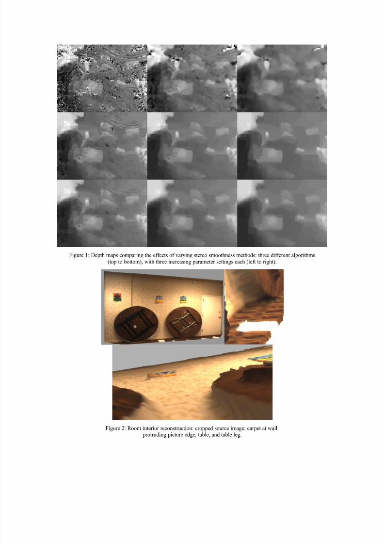
Figure 1 compares the effects of smoothness method 0 with varying filter sizes and methods 1 and 2 with varying

smoothness weights, in the presence of areas of weak texture (e.g., the building in the top left corner). With method 0(top), ambiguous texture is resolved by increasing the size of the (approximately circular) window. With methods 1

(middle) and 2 (bottom), ambiguous texture is resolved by increasing the weight of the smoothness term. It can be seenthat, in poorly textured regions, method 0 continues to yield gross outliers long after fine details are obliterated, while

methods 1 and 2 produce results that are both less noisy and more detailed. In regions where true depth varies smoothlyacross multiple hypothesized planes (e.g., any non-horizontal surface), the smoother results of method 2 further improve

upon the somewhat blocky results of method 1.

In terms of computational complexity, method 0 only involves independent univariate optimizations, and so is extremely

simple. Methods 1 and 2 optimize all unknowns simultaneously and are conceptually very similar to each other, but

method 2 uses five times as many unknowns to implement its additional smoothness term. Because the memory

requirements of method 1 already strain typical desktop computers, method 2 makes a further space-time compromise.



Applying our current implementations to a typical problem size of 480 × 320 × 60, method 1 (optimized to be fast) uses

600+ megabytes of virtual memory, while method 2 (optimized to be compact) uses 700+ megabytes, or much less than

five times as much; but method 2 is 25–30 times slower than method 1, which is in turn 10–15 times slower than

method 0. (For all three smoothness methods, space and time requirements both scale approximately linearly with the

problem size.)



Figure 1: Depth maps comparing the effects of varying stereo smoothness methods: three different algorithms

(top to bottom), with three increasing parameter settings each (left to right).

Figure 2: Room interior reconstruction: cropped source image; carpet at wall; protruding picture edge, table, and table leg.



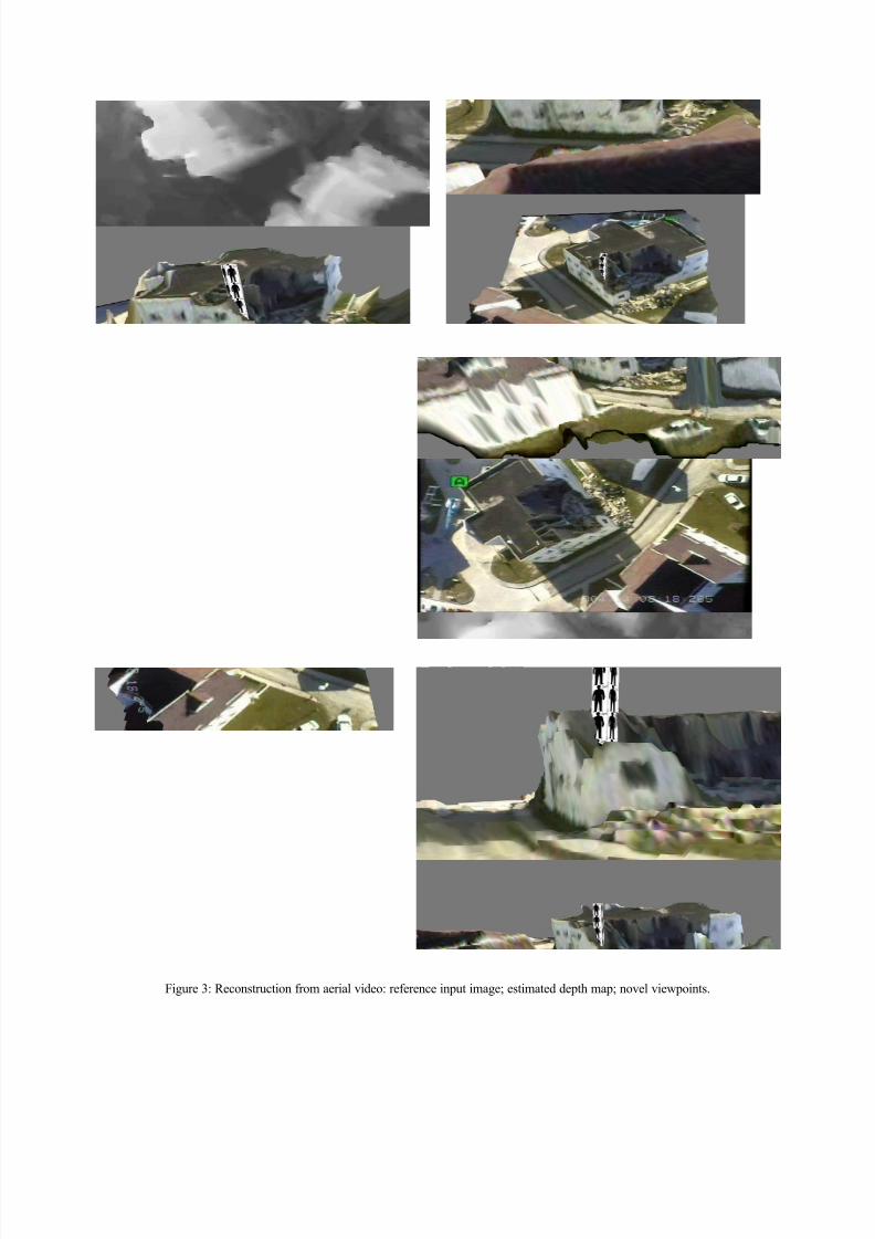
Figure 3: Reconstruction from aerial video: reference input image; estimated depth map; novel viewpoints.



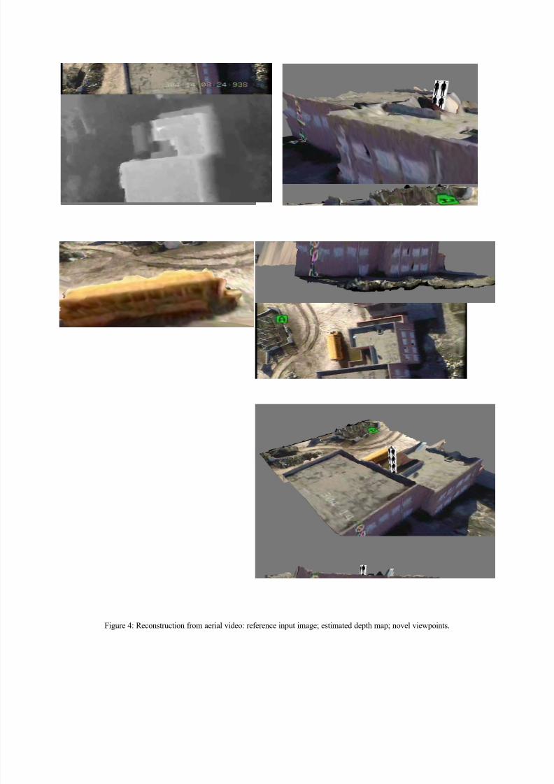
Figure 4: Reconstruction from aerial video: reference input image; estimated depth map; novel viewpoints.



6. RENDERING

In this module, we aim to generate viewable 3D models, in a format that can be rendered with off-the-shelf PC graphics

processors and tools. This requires not only the scene geometry, which is given by multi-view stereo, but also some way

of coloring or shading the rendered model.

Currently, we generate one polygonal mesh surface per multi-view stereo result. Because our stereo method estimates a

depth for each pixel in a reference view, there is a natural 2D ordering to the resulting 3D point cloud. This ordering cangenerally be taken to be equivalent to connectivity, except at depth discontinuities, where points adjacent in 2D image

space should be disconnected in 3D world space. Our meshing software tentatively generates the complete quadrilateral

mesh under the assumption that discontinuities do not exist, then removes any facet that is either too long in any

dimension or excessively oblique to the viewing direction of the reference view, before returning the remaining facets asthe estimated surface geometry. In our preliminary experiments, this method for estimating discontinuities has workedreasonably well, but we have disabled it for all of the results presented in this paper, in order to show the native output of

our stereo algorithm more clearly.

In our multi-view stereo method, the calculation of the variance volume could readily save the mean as well as thevariance at each 3D position; these values could then be used to color the estimated depth surface. This wouldautomatically combine multiple images to “erase” the camcorder annotations, but would be limited to producing color values in one-to-one correspondence with depth values. Because human perception is generally more sensitive to details

in color than in shape, we instead texture-map each estimated surface directly from the reference image used while

generating the corresponding stereo result, allowing us more flexibility to choose independent shape and color

resolutions according to computational and perceptual requirements.

Our end results combine surface mesh geometries and color texture maps into models interactively viewable by the

MeshView program distributed as part of Microsoft's DirectX software development kit.

7. RESULTS

Figure 2 shows a sample result from our first application, targeting handheld video of sparsely furnished room interiors.

This wall was reconstructed at a depth resolution of 1 cm. It can be seen in the detailed views from different

perspectives that the flatness of the wall and the perpendicularity of the floor are both recovered, as are the irregular

shapes of the round folding table, its folded legs, and the small pictures taped to the wall.

Figures 3 and 4 each show one multi-view stereo result from our second application, targeting aerial video of naturalterrain with manmade structures. These figures comprise the reference input view (top left), the estimated depth map

(top right), and several screenshots of the resulting surface rendered from various novel viewpoints (bottom). Columnsof stacked “people” have been inserted into the renderings to give a rough sense of the estimated scale; each “person” is

2 meters tall. These two results were both generated at a resolution of 480 × 320 × 60, using smoothness method 2, with

identical weights of the smoothness term, from 20-40 input images each.

In Figure 3, the lamp post is estimated to be much fatter than it should be, due to the convex smoothness term in

combination with our image pre-filtering and naive meshing algorithm. However, the remainder of these results

otherwise generally look good, with fairly flat ground, roof, and wall planes, as well as reasonable approximations to

such details as the piles of rubble (Figure 3) and the small rooftop walls (Figure 4).

8. FUTURE WORK

With our current software, achieving gap-free coverage requires stereo reconstruction from many, overlapping referenceviews; the result will represent each part of the terrain as many times as it is seen. One obvious approach to reducing this

redundancy would be to perform mesh merging and simplification [7]. Before such mesh merging, however, it would be

better if multiple representations of the same part of the terrain can be guaranteed to be consistent. Such consistency, aswell as the accuracy, of stereo results can be improved by considering multiple reference views within, rather than only

after, the stereo process [8]. Similarly, reconstruction of terrain from multiple independent videos could be used to

combine data from multiple passes over an area, or from multiple aerial platforms, into a single reconstruction with

minimal redundancy. We see two main areas that would need to be addressed before this can be done successfully.



First, in the absence of perfect position and orientation data, different video clips would have to be registered via other

means. For the best results, our feature tracker would need to be extended to find correspondences between, as well as

within, individual video clips; and our calibration methods would need to be extended to use this additional data to

estimate focal lengths and angular offsets that are separate for each clip, yet consistent among all clips. Alternatively, we

could merge results from different clips by attempting to align the recovered 3D geometry of each; this approach would

provide fewer alignment constraints, but might be simpler and/or more robust.

Then, once these enhancements give sufficiently accurate motion to enable multi-clip multi-view stereo, the stereoalgorithm itself would also need be generalized. At the minimum, it would need to handle large occluded areas, whichcannot be ignored in a wide baseline situation [9–10]. It would also be helpful to handle unoccluded areas that

nevertheless change appearance, both with viewing angle (e.g., specularities) and with time (e.g., variable cloud cover).

The aerial 3D reconstructions presented in this paper were calculated at a resolution of 480 × 320 × 60 samples each,

using video frames containing 720 × 480 pixels each. This corresponds to one sample per 1.5 video pixels in the image plane, and one sample per 10 to 20 cm in absolute elevation, depending on the range of elevations in the specific scene.

These height quanta are ~0.08% of a typical viewing standoff of ~250 meters at a viewing angle of ~45°, whichcorresponds to ~0.6 video pixels of image plane disparity resolution across the total image width. The primary limiting

factor that precluded higher resolutions was the large amount of memory required by the stereo algorithms. This

bottleneck can be alleviated by multi-resolution, pyramid-based methods, which generally reduce requirements in both

space and time, at the expense of weakening the optimality of the computed solution. How to minimize such

degradation of optimality is a subject of ongoing but promising research [11]. Further reduction of computational loadcould be achieved by simplifying the stereo smoothness constraints [12–13].

ACKNOWLEDGMENTS

This work was funded by DARPA contract W31P4Q-04-C-R186 and Air Force contract FA8651-04-C-0246. The

feature tracking algorithms and software were developed jointly with PercepTek and the Colorado School of Mines.

Thanks also to the authors of [1,2,5,6] for making their ready-to-use software components publicly available.

REFERENCES

[1] Jean-Yves Bouguet, “Camera Calibration Toolbox for Matlab,” 2003. http://www.vision.caltech.edu/bouguetj/calib_doc/

[2] Manolis I.A. Lourakis, Antonis A. Argyros, “The Design and Implementation of a Generic Sparse Bundle Adjustment Software

Package Based on the Levenberg - Marquardt Algorithm,” ICS / FORTH Technical Report No. 340, Aug. 2004.http://www.ics.forth.gr/~lourakis/sba/

[3] Junhwan Kim, Vladimir Kolmogorov, Ramin Zabih, “Visual Correspondence Using Energy Minimization and MutualInformation,” ICCV 2003.

[4] Olga Veksler, “Efficient Graph-Based Energy Minimization Methods in Computer Vision,” PhD thesis, Aug. 1999.

[5] Yuri Boykov, Vladimir Kolmogorov, “An Experimental Comparison of Min-Cut / Max-Flow Algorithms for EnergyMinimization in Computer Vision,” IEEE Trans. PAMI, Sept. 2004. http://www.cs.cornell.edu/People/vnk/software.html

[6] Sylvain Paris, Francois Sillion, Long Quan, “A Surface Reconstruction Method Using Global Graph Cut Optimization,” IJCV2005.

[7] Brian Curless, Marc Levoy, “A Volumetric Method for Building Complex Models from Range Images,” SIGGRAPH 1996.http://graphics.stanford.edu/software/vrip/

[8] Yanghai Tsin, “Kernel Correlation as an Affinity Measure in Point-Sampled Vision Problems,” PhD thesis, Sept. 2003.

[9] Sing Bing Kang, Richard Szeliski, Jinxiang Chai, “Handling Occlusions in Dense Multi-view Stereo,” CVPR 2001.

[10] Yichen Wei, Long Quan, “Asymmetrical Occlusion Handling Using Graph Cut for Multi-View Stereo,” CVPR 2005.

[11] Sebastien Roy, Marc-Antoine Drouin, “Non-Uniform Hierarchical Pyramid Stereo for Large Images,” Vision, Modeling, andVisualization 2002.

[12] Heiko Hirschmüller, “Accurate and Efficient Stereo Processing by Semi-Global Matching and Mutual Information,” CVPR 2005.

[13] Olga Veksler, “Stereo Correspondence by Dynamic Programming on a Tree,” CVPR 2005.

Documents

3d Environement Capture From Mono Video and Inertial Data