Embed Size (px)
Citation preview
3D FREQUENCY-DOMAIN SEISMIC INVERSION WITHCONTROLLED SLOPPINESS.
TRISTAN VAN LEEUWEN∗ AND FELIX J. HERRMANN†
Abstract. Seismic waveform inversion aims at obtaining detailed estimates of subsurfacemedium parameters, such as the spatial distribution of soundspeed, from multi-experiment seis-mic data. A formulation of this inverse problem in the frequency-domain leads to an optimizationproblem constrained by a Helmholtz equation with many right-hand-sides.
Application of this technique to industry-scale problem faces several challenges: Firstly, we needto solve the Helmholtz equation for high wavenumbers over large computational domains. Secondly,the data consists of many independent experiments, leading to a large number of PDE-solves. Thisresults in high computational complexity both in terms of memory and CPU time as well as i/ocosts. Finally, the inverse problem is highly non-linear and a lot of art goes into preprocessing andregularization. Ideally, an inversion needs to be run several times with different initial guesses and/ortuning parameters.
In this paper, we discuss the requirements of the various components (PDE-solver, optimizationmethod, ...) when applied to large-scale 3D seismic waveform inversion and combine several existingapproaches into a flexible inversion scheme for seismic waveform inversion. The scheme is basedon the idea that in the early stages of the inversion we do not need all the data or very accuratePDE-solves. We base our method on an existing preconditioned Krylov solver (CARP-CG) anduse ideas from stochastic optimization to formulate a gradient-based (Quasi-Newton) optimizationalgorithm that works with small subsets of the right-hand-sides and uses inexact PDE solves for thegradient calculations. We proposed novel heuristics to adaptively control both the accuracy and thenumber of right-hand-sides. We illustrate the algorithms on synthetic benchmark models for whichsignificant computational gains can be made without being sensitive to noise and without loosingaccuracy of the inverted model.
Key words. Seismic inversion, Helmholtz equation, preconditioning, Kaczmarz method, inexactgradient, block-cg
1. Introduction. Detailed estimates of subsurface properties such as sound-speed and density can be obtained from seismic data by solving a PDE-constrainedoptimization problem [44]—also known as full-waveform inversion (FWI) in the seis-mic community —that involves multiple source experiments. The data in this settingconsist of a collection of time-series for many source-receiver pairs and are the resultof either passive or active source experiments. The PDE is a wave-equation with asmany right-hand-sides as there are sources. Applications of this technique include oiland gas exploration and global seismology. A common characteristic of these appli-cations is the need to propagate the waves over large distances (i.e., several hundredwavelenghts) through strongly inhomogeneous media for a large number of sources.This leads to a non-linear data-fitting problem involving millions, and in industrialsettings even billions, of unknowns and exceedingly large data volumes (up to ∼ 1015
data-points).While the FWI problem is naturally formulated in the time-domain, we can for-
mulate an equivalent problem in the frequency-domain by applying a temporal Fouriertransform to the observed data and using the Helmholtz equation to predict the data.One of the main reasons to do this is that it allows us to work with relatively smalldata volumes (i.e., a few frequencies instead of the whole time-series). This formu-lation also avoids the need for i/o-intensive checkpointing schemes when employing
∗Centrum Wiskunde & Informatica (CWI), Amsterdam, The Netherlands([email protected]). Formerly at ††Dept. of Earth, Ocean and Atmospheric sciences. University of British Columbia. Vancouver,
BC, Canada ([email protected])
1
adjoint-state methods [42]. While iteratively solving the Helmholtz equation in 3D isstill a challenge, recent benchmark tests suggest that it is becoming competitive whencompared to time-stepping methods [25].
Although conceptually attractive, this straightforward data-fitting approach toseismic inversion is plagued by the severe non-linear relation between the data andunknown medium parameters. In particular, the oscillatory nature of the data mayresult in a partial fit even though the medium parameters do not represent the trueearth. This phenomena is known as loop-skipping and may cause gradient-based op-timization methods to fail because they get stuck in a local minimum (see [43] foran overview). Many alternative formulations of the inverse problem have been pro-posed to mitigate this problem [51]. These formulations rely either on using differentobjective functions to measure the data-misfit [27, 52] or on completely different for-mulations of the inverse problem [41, 34, 50]. While less sophisticated than the afore-mentioned methods, a simple remedy is based on the observation that loop-skipping isless of a problem at low frequencies. This observation motivated [6, 37, 53] to proposea multi-scale continuation method where the inversion is carried out from low to highfrequencies. Needless to say, this multiscale approach is trivially implemented in thefrequency-domain.
PDE-constrained optimization problems can be solved in a variety of ways, viaeither Lagrange methods or SQP [19]. All these methods rely – in one way or an-other – on simultaneously updates of both the state and control variables, and thusavoids having to explicitly solve the PDE. Unfortunately, the scale of typical seismicproblems, even in 2D, precludes the use of such full-space methods because it requiressimultaneous storage of the forward and adjoint wavefields for all sources. For thatreason, practitioners usually resort to reduced-space methods that rely on explicitlyeliminating the state variables [36, 10] by solving the PDE for each gradient update.The gradient of the reduced objective with respect to the medium parameters canthen be efficiently computed via the adjoint-state method [44, 33].
For 2D applications, the discretized PDE (the Helmholtz equation) is usually fac-torized and its inverse can thus be applied cheaply to multiple right-hand-sides. In3D, however, direct factorization does not scale very well to large problems due tothe memory requirements caused by the large number of gridpoints needed and theincreased bandwidth of the matrix. This poses major problems when applying 3Dwaveform inversion to industry-scale datasets: i) The Helmholtz equation is notori-ously difficult to solve due to the indefiniteness and requires sophisticated precondi-tioners (see [12] for an extensive overview). This is a very active area of research andmany preconditioners have been proposed. However, many of these approaches areproblem specific, require (manual) tuning of problem-specific parameters to ensureconvergence, and may suffer from significant setup and memory storage costs. Whilewell-suited for very accurate simulation with fixed medium parameters, these dedi-cated approaches are not particularly attractive for inversion where the coefficientsin the PDE change after every model update. ii) The computational costs scalelinearly with the number of sources, which in realistic settings makes even a singlegradient computation prohibitively expensive. Recently, techniques from stochasticoptimization have been applied to dramatically reduce the computational cost bylowering the number of right-hand-sides via random projections or random subsam-pling [20, 46, 49, 55]. Aside from decreasing the computational cost by reducing therequired number of PDE solves, these approaches also decrease the computationaloverhead related to i/o. Although this approach can lead to significant reduction
2
of the per-iteration cost of gradient-based optimization algorithms, these stochasticmethods have the disadvantage that they often lead to a sub-linear convergence andhence may require disproportionally more iterations to converge. In theory, this loss ofconvergence can be overcome by gradually increasing the sample-size [13] by bringingin more right-hand-sides. The rate with which the sample-size needs to be increaseddepends on problem-specific constants that are expensive to compute in practice.Hence, there is a need for an adaptive strategy based on heuristics that are easy tocompute. Inexactness is another powerful tool for reducing the computational costswhen using iterative methods to solve the PDEs [23, 4, 22]. It is not clear how tochoose the tolerance of the inexact PDE solves such that the computations are stillsufficiently accurate to be usefull.
To carry out our data-intensive large-scale inversions based on local derivatives,iterative 3D PDE solves for time-harmonic Helmholtz, and stochastic optimization,we propose that a scalable – both in terms of data and model-size – inversion strategyneeds to consist of the following key ingredients:
• an iterative Helmholtz solver with low memory imprint and computationaloverhead, e.g. setup costs, whose convergence does not critically depend onmodel-dependent tuning parameters,
• a practical stopping criterion for the iterative solver that avoids computingaccurate solutions when they are not needed – e.g. when the model iterate isfar from the true solution,
• a (stochastic) optimization strategy that exploits the separable structureof the objective by working with small subsets of the right-hand-sides at eachiteration,
• a criterion to adaptively grow the sample-size as the optimization proceeds,and
• the ability to exploit both model-space, via domain decomposition, anddata-space parallelism, by parallelizing loops over frequencies and / orright-hand-sides.
Because practical application of full waveform inversion to field data still requiresa lot parameter tuning and careful selection of the initial model, the ultimate goalis to reduce the turnaround time for a typical inversion. This would allow us to runmultiple scenarios to test the validity of the output.
1.1. Contributions. In this paper, we propose a new comprehensive frameworkfor 3D seismic waveform inversion that addresses both the need to efficiently solve theHelmholtz equation as well as the computational cost induced by the many right-hand-sides. To this end, we combine several existing components into a novel algorithmthat addresses these issues by developing practical algorithms designed to scale wellby exploiting data- as well as model-space parallelism.
Helmholtz solver. Because of its relative simplicity, flexibility towards differentwave physics, and robustness with respect to tuning parameter selection, we investi-gate the use of an existing Kaczmarz-based preconditioned iterative method (CGMN)and more specifically its parallel extensions (CARP-CG). We evaluate the perfor-mance of this solver in the context of inversion. Because we are dealing with multipleright-hand sides, we incorporate the preconditioner in a block-iterative method andevaluate its performance.
Inexact PDE-solves. To reduce the computational cost of the inversion, weconsider an inexact approach which solves the PDEs up to some relatively high pre-
3
scribed tolerance. We propose a novel heuristic to adaptively determine the requiredaccuracy of the PDE solves based on the data-misfit.
Source subsampling and stochastic optimization. We further reduce thecomputational cost by working with small subsets of the sources at each iteration andpropose a novel heuristic to determine whether the sample size needs to be increasedbased on an average descent of the (sampled) objective.
The result is a new adaptive stochastic quasi-Newton optimization method forseismic inversion that automatically determines the required accuracy for the PDEsolves and automatically increases the sample-size when an average descent conditionfails. Since accuracy is really a proxy for computational costs, the basic motto of ourapproach is to never use more accuracy than strictly needed at any point during theinversion. This leads to significant reductions in the number of right-hand-sides forthe gradient calculations and in the number of iterations for the Helmholtz solves.
1.2. Outline. In section 2, we discuss the discretization of the Helmholtz equa-tion and the Kaczmarz-based preconditioner. Section 3 describes the stochastic inver-sion strategy and the heuristics used to determined the accuracy of the PDE solvesand the sample-size. Some numerical experiments are presented in section 4 andsection 5 presents conclusions and discussions.
2. Modeling. We model wave-propagation in the earth via the following 3Dscalar Helmholtz equation,[
ω2
c(x)2ρ(x)+∇ · 1
ρ(x)∇]u(ω, x) = s(ω, x) + b.c.′s, (2.1)
where ω is the frequency, x is the spatial coordinate, c(x) denotes the soundspeedρ(x) denotes the density, u(ω, x) denotes the wavefield and s(ω, x) is a source term.
We discretize the Helmholtz equation using a a 27-point mixed-grid stencil withPML boundary conditions on all sides of the domain [31] and denote the resultingsparse linear system by
Au = s, (2.2)
where u and s denote the gridded wavefield and source function.
2.1. Iterative solver. Due to the sheer size of typical problems in 3D seismicimaging (∼ 109 gridpoints), direct factorization techniques are not widely used. Re-cent work by Wang et al. [54] aims at reducing the memory imprint by employinghierarchical low-rank (HSS) representations of the factorization. Even taking thesenew developments into account, direct factorization techniques are not practical forthe proposed inversion scheme since the initial factorization costs cannot be amortizedover a large number of sources (we will focus on the use of optimization methods thatuse only a relatively small number of right-hand-sides at each iteration). Moreover,the massively parallel implementation required for such direct methods precludes theuse of course-scale parallelism (e.g., parallelizing over sources and / or frequencies).Moreover, a new factorization will be needed after each model-update.
Iterative techniques are much more efficient in terms of memory use, and aremore attractive when using only a relatively small number of right-hand-sides. How-ever, they require a good preconditioner. Many preconditioning techniques have beenproposed in the literature [11, 38, 32, 21, 9, 40, 35]. Most of these are designed
4
for efficient and accurate forward modeling and include problem-specific tuning pa-rameters to ensure convergence. The latter does not make these approaches veryattractive for inversion since the medium parameters will change from one iterationto the next, possibly requiring the tuning-parameters to be changed as well. Instead,we use CARP-CG [14, 15], a generic, iterative solution technique for sparse linearsystems based on the CGMN method [5]. Convergence of this method is guaranteed,making it an attractive solver for inversion purposes. Moreover, the method is genericand can thus be applied to other discretisations or even vector-Helmholtz equationswithout any modification.
Naively, one can think of this method as a Kaczmarz-preconditioned conjugategradient (CG) method. For the sake of completeness, we give a brief overview of themethod.
CGMN. The Kaczmarz method solves a system of N equations, Au = s, bycyclically projecting the iterate onto rows of the matrix [24]
u := u + γ (si − ai∗u)ai/||ai||22, i = 1 . . . N, (2.3)
where ai denotes the i-th row of A as column vector, ·∗ denotes the conjugatetranspose, and 0 < γ < 2 is a relaxation parameter. Introducing the matricesQi =
(I − γaiai∗/||ai||22
), we may write this iteration as
u := Qiu + γsiai/||ai||22.
A double sweep through the matrix (from row 1 to N and back) can then be denotedby
u := Qu +Rs,
where Q = Q1Q2 . . . QNQN . . . Q1 and R contains all the factors multiplying s. It iseasily verified that the Qi are Hermitian rank 1 matrices with eigenvalue 1 − γ. Itfollows that Q is Hermitian and has eigenvalues ∈ (−1, 1).
We may now transform the original system of equations to a Hermitian positivesemi-definite system:
(I −Q)u = Rs,
which we can solve with the CG method.Since this preconditioner is equivalent to SSOR on the normal equations AA∗ [5],
we find the following alternative expressions for Q and R
Q = I −A∗HA, (2.4)
R = A∗H. (2.5)
with H = γ(2− γ) (D + γL∗)−1D (D + γL)
−1, where D and L contain the diagonal
and lower triangular elements of AA∗. Although these expressions are convenientfor analysis and testing, a more efficient implementation computes only the action ofthese matrices using Algorithm 1 as Qu +Rs = DKSWP(A,u, s, γ) [14].
The choice of the parameter γ does not seem to critically affect the convergence,although values γ ≈ 1.5 appear to be optimal (see, for example, [16] for extensivenumerical experiments). A Fourier analysis for the 1D Helmholtz equation of theCGMN method confirms this [47].
Finally, the method lends itself for a matrix-free implementation where the stencilcoefficients are generated on-the-fly. This will be important when moving to higher-order stencils where we cannot afford to store all the stencil coefficients.
5
Algorithm 1 DKSWP(A,u, s, γ) Performs a forward and backward Kaczmarz sweepon the matrix A{forward sweep}for i = 1 to N dou := u + γ(si − ai
∗u)ai/||ai||22end for{backward sweep}for i = N to 1 dou := u + γ(si − ai
∗u)ai/||ai||22end forreturn u
Block-CG. Since we are mostly dealing with multiple right-hand-sides simul-taneously, we use a block-CG method [3, 18] to solve the Helmholtz equation formultiple right-hand-sides simultaneously. By building up a Krylov subspace usingmultiple residual vectors simultaneously, block-iterative methods may converge sig-nificantly faster at the cost of an increased computational cost per iteration. It iswell-known that block iterative methods will break down if the residual vectors be-come linearly dependent. To counter this, a re-orthogonalization of the residuals inconjunction with so-called variable-block or deflation techniques can be used [3, 29, 8].However, since the right-hand-sides in our case represent different sources we expectthe initial residuals to be nearly orthogonal. In our experiments we typically reach thedesired tolerance – which is usually high – before any linear dependence between theresiduals develops. The resulting algorithm – without deflation – is given in algorithm2 (adapted from [18], algorithm 8.). For a more robust implementation, variable-blockor deflation techniques can be added.
Algorithm 2 BCGMN(A,U0, S, γ, ε) Block-CGMN algorithm on system AU = Susing DKSWP to perform the matrix-vector multiplications
P0 = R0 = DKSWP(A,U0, S, γ)− U0
while ||Rk||F > ε||R0||F doQk = Pk − DKSWP(A,Pk, 0, γ)αk = (Pk
∗Qk)−1(Rk∗Rk)
Uk+1 = Uk + Pkαk
Rk+1 = Rk −Qkαk
βk = (Rk∗Rk)−1(Rk+1
∗Rk+1)Pk+1 = Rk + Pkβkk = k + 1
end while
Domain decomposition. The CARP-CG algorithm is a parallel extension ofthe CGMN algorithm, where the Kaczmarz projections are done independently andin parallel on blocks of rows. Between each sweep through the rows, the overlappingelements of the solutions are averaged. As such, its implementation resembles anadditive Schwarz approach, however, CARP-CG is guaranteed to converge. For detailswe refer the reader to [14, 15]. The use of CARP-CG to solve the Helmholtz equationspecifically is described by [16, 17].
In summary, we discussed a generic, solver for the Helmholtz equation with mul-
6
tiple right-hand sides. Because convergence of the method does not critically dependon tuning parameters, this method is suitable for inversion. Some numerical exper-iments and a comparison to other simple iterative methods are presented in section4.1.
3. Inversion. The inverse problem for M sources and a single frequency can becast as a PDE-constrained optimization problem
minm,w,u
M∑i=1
ρ(wiPiui − di
)s.t. A(m)ui = si, (3.1)
where ρ is a (differentiable) penalty function, m denotes the model parameter ofinterest (i.e, velocity, density or some combination of thereof), A is the discretizedHelmholtz operator, u = [u1; . . . ;uM ] are the wavefields for sources s = [s1; . . . ; sM ],Pi is a detection operator, w is a vector of source weights and d = [d1; . . . ;dM ] arethe observed data.
Standard all-at-once approaches to solving this PDE-constrained optimizationproblem rely on a Lagrangian formulation of this problem
L(m,w,u,v) =M∑i=1
ρ(wiPiui − di
)+ v∗i
(A(m)ui − si
), (3.2)
and use a Newton-like method to solve ∇L = 0, where
∇uiL = P ∗i ∇ρ(wiPiui − di
)+A(m)∗vi, (3.3)
∇viL = A(m)ui − si, (3.4)
∇wiL =(Piui
)∗∇ρ(wiPiui − di
)(3.5)
∇mL =
M∑i=1
G(m,ui)∗vi, (3.6)
where G(m,ui) = ∂A(m)ui
∂m . Updating both state and control variables is not feasiblefor such large-scale problems so we use a so-called reduced approach, eliminating thestate variables ui and vi by solving the forward (∇vi
L = 0) and adjoint (∇uiL = 0)
PDEs. We simplify the problem even further by projecting out w. This can be doneefficiently by solving a series of scalar optimization problems [2]
wi = argminw
ρ(wPiui − di
). (3.7)
Finally, the reduced objective is given by
φ(m) =
M∑i=1
φi(m), φi(m) = ρ(wiPiui − di
). (3.8)
Note that the evaluation of the reduced objective requires the solution of the forwardPDE (3.4) as well as the solution of M scalar optimization problems (3.7). Thegradient of φ coincides with the gradient of the Lagrangian w.r.t. m (3.6) evaluatedat the optimal ui, vi and w and thus requires the additional solution of an adjointPDE (3.3).
7
3.1. Gradient-descent with errors. A basic gradient-descent algorithm tominimize φ(m) is based on the iteration
mk+1 = mk − νk∇φ(mk), (3.9)
where νk is the stepsize. However, the evaluation of the reduced objective (3.8) andits gradient requires 2M PDE solves, which may be prohibitively large. To reducethese costs, we resort to an optimization technique described by [13] that allows forthe use of approximate gradients in a gradient descent algorithm:
mk+1 = mk − νkgk, (3.10)
where gk = ∇φ(mk) + ek is the approximate gradient and ek is the approximationerror. Specifically, [13, Thm 2.2] proves that under some convexity assumptions onthe objective function φ(m) and for an appropriately chosen fixed stepsize, a basicgradient-descent algorithm with approximate gradients (3.10) will converge as
φ(mk)− φ(m∗) < ak(φ(m0)− φ(m∗)),
where ak = max{ck, ||ek||22}, where 0 ≤ c < 1 depends on the condition number ofφ (c close to one being ill-conditioned). Thus, if the error in the gradient decreaseslinearly, the resulting gradient-descent algorithm with approximate gradients will alsoconverge linearly. Furthermore, this tells us that we need not decrease the accuracyvery fast if the problem is ill-conditioned to begin with (i.e., if c is close to one).
Of course, our objective is not very likely to satisfy these convexity assumptionsglobally, however, for the sake of designing an algorithm we will assume them to holdlocally.
Source subsampling. We can obtain approximate gradients with controllableerror by using only a subset of terms I ⊆ {1, 2, . . . ,M} in (3.8) when calculatingthe gradient. This sample average approach is extensively analyzed by [13, 1]. Ifwe choose the elements in I randomly from [1, 2, . . . ,M ] (without replacement), theexpected error in the gradient can be expressed as ||e||2 ∝
√b−1 −M−1 [13, section
3.2]. The computational cost is directly proportional to the sample size b = |I|, andthus a higher error in the gradient directly translates into a lower computational cost.Numerical experiments have shown that this approach is beneficial on 2D seismicinversion problems [49, 28]. How to choose the rate of increase of the sample-sizein practice is an open problem. Van den Doel et al. [46] suggest a cross-validationtechnique that relies on computing the objective for two independent samples andrequiring decrease on both. When this condition fails, the authors suggest to doublethe sample-size. This leads to an exponentially increasing sample-size and induces alot of computational overhead since all the computations are carried out twice.
We adopt a related approach that induces less computational overhead and in-creases the sample-size at a slower (linear) rate; we re-draw the samples at eachiteration and use the misfit for both the old and new samples to keep track of the av-erage descent. If the objective fails to decrease on average, we increase the sample-sizeby a constant amount. Details of the implementation in the context of an L-BFGSmethod are described in section 3.3.
3.2. Approximate PDE solves. In addition to using source-subsampling tech-niques to reduce the computational cost, we can solve the forward and adjoint PDEsup to some (high) tolerance ε. The crux lies in determining a reasonable ε. The use
8
of inexact PDE solves in the context of trust-region methods is discussed by [23, 22],while [4] discuss inexactness issues in full-space approaches.
Here we propose a heuristic to estimate a reasonable tolerance that is ‘accurateenough’ and is completely independent from the optimization strategy and allows forthe use of black-box optimization methods. The heuristic is based on the behavior ofthe objective for a single experiment as a function of the tolerance
φi(m, ε) = ρ(wiPiui(ε)− di
),
where ui(ε) is obtained by solving the forward PDE with tolerance ε (i.e., ||Aui(ε)−si||2 ≤ ε||si||2). We propose to choose a tolerance that computes the residual to withina certain fraction η of its true value, i.e., find an ε such that
|φi(m, ε)− φi(m, 0)| ≤ ηφi(m, 0).
This is not very practical since it would require a very accurate solve (with ε = 0).Instead, we find a k such that
|φi(m, αkε)− φi(m, αk+1ε)| ≤ ηφi(m, αk+1ε),
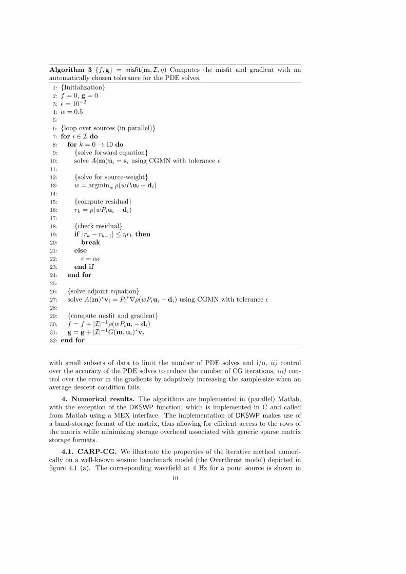
where α < 1. The resulting algorithm to evaluate the objective for a given sample Iis shown in Algorithm 3. We use the current solution, ui(α
kε), as initial guess whensolving solving for ui(α
k+1ε) in line 9. We use the same tolerance when solving theadjoint PDE.
Of course, a similar heuristic can be used to estimate the actual error in thegradient by finding a k such that
||gi(αkε)− gi(α
k+1ε)||2 ≤ η||gi(αk+1ε)||2,
where gi(ε) = G(m,ui(ε))∗vi(ε) and vi(ε) is obtained by solving the adjoint PDE up
to ε. Perhaps it would be even better to use a two different tolerances for the forwardand adjoint PDEs, but seen that the heuristic based on the misfit yielded very goodresults, we will leave detailed comparison of these two heuristics for future research.
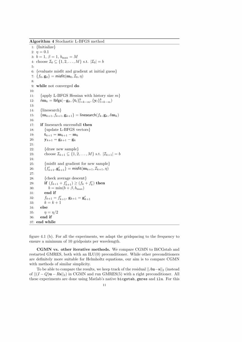
3.3. A stochastic Quasi-Newton algorithm. We incorporate the heuristicsdescribed above in a novel stochastic Quasi-Newton algorithm. Aside from using onlya subset of the sources and approximate PDE solves, we re-draw the sample at eachiteration, even if the sample-size does not increase. Such a renewal of the sampleremoves any possible bias introduced by using a particular subset and has provedhighly beneficial in seismic applications [48, 26].
The algorithm decreases η when the linesearch fails and increases the sample-size when the average objective as computed over two independent samples does notdecrease. A detailed description is given in Algorithm 4.
The objective values f ′k and f ′k+1 in line 29 are computed using different samplesbecause the samples themselves are renewed at each iteration (cf. line 23), even if thesample-size remains unchanged.
For the linesearch (line 15) we use a weak Wolfe linesearch and lbfgs (line 12)applies the L-BFGS scaling based on past gradient and model updates (cf. lines19,20) [30]. Note that the Hessian update requires an extra gradient computationsince we want to compute the update vectors yk (line 20) from gradients that werecomputed for the same sample I [39, 7].
The above described adaptive stochastic algorithm combines several featuresneeded to solve large-scale seismic inversion problems. These include: i) working
9
Algorithm 3 {f,g} = misfit(m, I, η) Computes the misfit and gradient with anautomatically chosen tolerance for the PDE solves.
1: {Initialization}2: f = 0, g = 03: ε = 10−2
4: α = 0.55:
6: {loop over sources (in parallel)}7: for i ∈ I do8: for k = 0→ 10 do9: {solve forward equation}
10: solve A(m)ui = si using CGMN with tolerance ε11:
12: {solve for source-weight}13: w = argminw ρ(wPiui − di)14:
15: {compute residual}16: rk = ρ(wPiui − di)17:
18: {check residual}19: if |rk − rk−1| ≤ ηrk then20: break21: else22: ε = αε23: end if24: end for25:
26: {solve adjoint equation}27: solve A(m)∗vi = Pi
∗∇ρ(wPiui − di) using CGMN with tolerance ε28:
29: {compute misfit and gradient}30: f = f + |I|−1ρ(wPiui − di)31: g = g + |I|−1G(m,ui)
∗vi
32: end for
with small subsets of data to limit the number of PDE solves and i/o, ii) controlover the accuracy of the PDE solves to reduce the number of CG iterations, iii) con-trol over the error in the gradients by adaptively increasing the sample-size when anaverage descent condition fails.
4. Numerical results. The algorithms are implemented in (parallel) Matlab,with the exception of the DKSWP function, which is implemented in C and calledfrom Matlab using a MEX interface. The implementation of DKSWP makes use ofa band-storage format of the matrix, thus allowing for efficient access to the rows ofthe matrix while minimizing storage overhead associated with generic sparse matrixstorage formats.
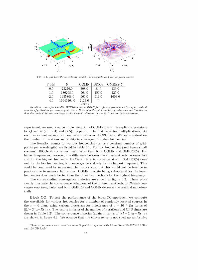
4.1. CARP-CG. We illustrate the properties of the iterative method numeri-cally on a well-known seismic benchmark model (the Overthrust model) depicted infigure 4.1 (a). The corresponding wavefield at 4 Hz for a point source is shown in
10
Algorithm 4 Stochastic L-BFGS method
1: {Initialize}2: η = 0.13: b = 1, β = 1, bmax = M4: choose I0 ⊆ {1, 2, . . . ,M} s.t. |I0| = b5:
6: {evaluate misfit and gradient at initial guess}7: {f0,g0} = misfit(m0, I0, η)8:
9: while not converged do10:
11: {apply L-BFGS Hessian with history size m}12: δmk = lbfgs(−gk, {tl}kl=k−m, {yl}kl=k−m)13:
14: {linesearch}15: {mk+1, fk+1,gk+1} = linesearch(fk,gk, δmk)16:
17: if linesearch successfull then18: {update L-BFGS vectors}19: tk+1 = mk+1 −mk
20: yk+1 = gk+1 − gk
21:
22: {draw new sample}23: choose Ik+1 ⊆ {1, 2, . . . ,M} s.t. |Ik+1| = b24:
25: {misfit and gradient for new sample}26: {f ′k+1,g
′k+1} = misfit(mk+1, Ik+1, η)
27:
28: {check average descent}29: if (fk+1 + f ′k+1) ≥ (fk + f ′k) then30: b = min(b+ β, bmax)31: end if32: fk+1 = f ′k+1, gk+1 = g′k+1
33: k = k + 134: else35: η = η/236: end if37: end while
figure 4.1 (b). For all the experiments, we adapt the gridspacing to the frequency toensure a minimum of 10 gridpoints per wavelength.
CGMN vs. other iterative methods. We compare CGMN to BiCGstab andrestarted GMRES, both with an ILU(0) preconditioner. While other preconditionersare definitely more suitable for Helmholtz equations, our aim is to compare CGMNwith methods of similar simplicity.
To be able to compare the results, we keep track of the residual ||Au−s||2 (insteadof ||(I −Q)u−Rs||2) in CGMN and run GMRES(5) with a right preconditioner. Allthese experiments are done using Matlab’s native bicgstab, gmres and ilu. For this
11
(a) (b)
Fig. 4.1. (a) Overthrust velocity model, (b) wavefield at 4 Hz for point-source
f [Hz] N CGMN BiCGs GMRES(5)0.5 23276.0 308.0 81.0 139.01.0 186208.0 564.0 150.0 425.02.0 1455808.0 960.0 911.0 1603.04.0 11646464.0 2123.0 * *
Table 4.1Iteration counts for CGMN, BiCGstab and GMRES for different frequencies (using a constant
number of gridpoints per wavelength). Here, N denotes the total number of unknowns and * indicatesthat the method did not converge to the desired tolerance of ε = 10−6 within 5000 iterations.
experiment, we used a naive implementation of CGMN using the explicit expressionsfor Q and R (cf. (2.4) and (2.5)) to perform the matrix-vector multiplications. Assuch, we cannot make a fair comparison in terms of CPU time. We focus instead onthe number of iterations and ability to converge for higher frequencies.
The iteration counts for various frequencies (using a constant number of grid-points per wavelength) are listed in table 4.1. For low frequencies (and hence smallsystems), BiCGstab converges much faster than both CGMN and GMRES(5). Forhigher frequencies, however, the difference between the three methods becomes lessand for the highest frequency, BiCGstab fails to converge at all. GMRES(5) doeswell for the low frequencies, but converges very slowly for the highest frequency. Thiscould be countered by increasing the history size, but this would not be feasible inpractice due to memory limitations. CGMN, despite being suboptimal for the lowerfrequencies does much better than the other two methods for the highest frequency.
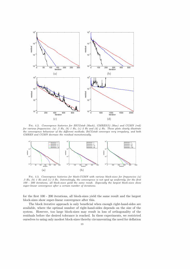
The corresponding convergence histories are shown in figure 4.2. These plotsclearly illustrate the convergence behaviour of the different methods; BiCGstab con-verges very irregularly, and both GMRES and CGMN decrease the residual monoton-ically.
Block-CG. To test the performance of the block-CG approach, we computethe wavefields for various frequencies for a number of randomly located sources inthe z = 0 plane using various blocksizes for a tolerance of ε = 10−6 (in terms of||(I−Q)u−Rs||F ). The results in terms of the number of iterations and CPU times areshown in Table 4.21. The convergence histories (again in terms of ||(I −Q)u−Rs||F )are shown in figure 4.3. We observe that the convergence is not sped up uniformly;
1These experiments were done Dual-core SuperMicro system with 2 Intel Xeon [email protected] Ghzand 128 GB RAM.
12
0 50 100 150 200 250 30010
−6
10−4
10−2
100
iteration
resid
ual
0 100 200 300 400 50010
−6
10−4
10−2
100
iteration
resid
ual
(a) (b)
0 200 400 600 80010
−6
10−4
10−2
100
iteration
resid
ual
0 500 1000 1500 200010
−6
10−4
10−2
100
iteration
resid
ual
(c) (d)
Fig. 4.2. Convergence histories for BICGstab (black), GMRES(5) (blue) and CGMN (red)for various frequencies: (a) .5 Hz, (b) 1 Hz, (c) 2 Hz and (d) 4 Hz. These plots clearly illustratethe convergence behaviour of the different methods; BiCGstab converges very irregulary, and bothGMRES and CGMN decrease the residual monotonically.
0 50 100 150 200 250 30010
−6
10−4
10−2
100
iteration
resid
ual
blocksize = 1
blocksize = 2
blocksize = 5
blocksize = 10
0 100 200 300 400 50010
−6
10−4
10−2
100
iteration
resid
ual
blocksize = 1
blocksize = 5
blocksize = 10
blocksize = 50
0 200 400 600 800 100010
−6
10−4
10−2
100
iteration
resid
ual
blocksize = 1
blocksize = 10
blocksize = 50
blocksize = 100
(a) (b)
Fig. 4.3. Convergence histories for block-CGMN with various block-sizes for frequencies (a).5 Hz, (b) 1 Hz and (c) 2 Hz. Interestingly, the convergence is not sped up uniformly; for the first100 - 200 iterations, all block-sizes yield the same result. Especially the largest block-sizes showsuper-linear convergence after a certain number of iterations.
for the first 100 - 200 iterations, all block-sizes yield the same result and the largestblock-sizes show super-linear convergence after this.
The block iterative approach is only beneficial when enough right-hand-sides areavailable, where the optimal number of right-hand-sides depends on the size of thesystem. However, too large block-sizes may result in loss of orthogonality of theresiduals before the desired tolerance is reached. In these experiments, we restrictedourselves to using only modest block-sizes thereby circumventing the need for deflation
13
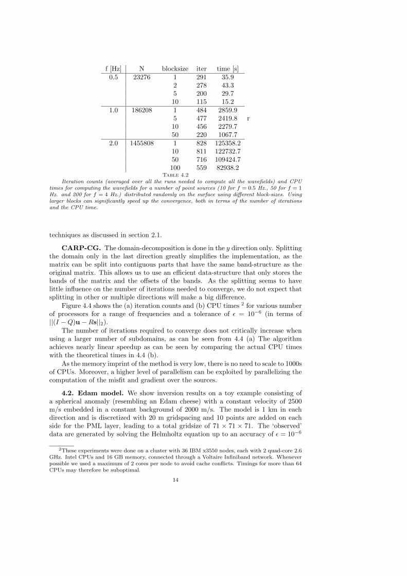
f [Hz] N blocksize iter time [s]0.5 23276 1 291 35.9
2 278 43.35 200 29.710 115 15.2
1.0 186208 1 484 2859.95 477 2419.810 456 2279.750 220 1067.7
2.0 1455808 1 828 125358.210 811 122732.750 716 109424.7100 559 82938.2
r
Table 4.2Iteration counts (averaged over all the runs needed to compute all the wavefields) and CPU
times for computing the wavefields for a number of point sources (10 for f = 0.5 Hz., 50 for f = 1Hz. and 200 for f = 4 Hz.) distributed randomly on the surface using different block-sizes. Usinglarger blocks can significantly speed up the convergence, both in terms of the number of iterationsand the CPU time.
techniques as discussed in section 2.1.
CARP-CG. The domain-decomposition is done in the y direction only. Splittingthe domain only in the last direction greatly simplifies the implementation, as thematrix can be split into contiguous parts that have the same band-structure as theoriginal matrix. This allows us to use an efficient data-structure that only stores thebands of the matrix and the offsets of the bands. As the splitting seems to havelittle influence on the number of iterations needed to converge, we do not expect thatsplitting in other or multiple directions will make a big difference.
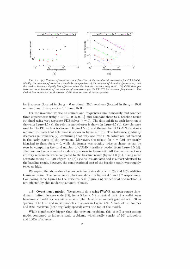
Figure 4.4 shows the (a) iteration counts and (b) CPU times 2 for various numberof processors for a range of frequencies and a tolerance of ε = 10−6 (in terms of||(I −Q)u−Rs||2).
The number of iterations required to converge does not critically increase whenusing a larger number of subdomains, as can be seen from 4.4 (a) The algorithmachieves nearly linear speedup as can be seen by comparing the actual CPU timeswith the theoretical times in 4.4 (b).
As the memory imprint of the method is very low, there is no need to scale to 1000sof CPUs. Moreover, a higher level of parallelism can be exploited by parallelizing thecomputation of the misfit and gradient over the sources.
4.2. Edam model. We show inversion results on a toy example consisting ofa spherical anomaly (resembling an Edam cheese) with a constant velocity of 2500m/s embedded in a constant background of 2000 m/s. The model is 1 km in eachdirection and is discretized with 20 m gridspacing and 10 points are added on eachside for the PML layer, leading to a total gridsize of 71 × 71 × 71. The ‘observed’data are generated by solving the Helmholtz equation up to an accuracy of ε = 10−6
2These experiments were done on a cluster with 36 IBM x3550 nodes, each with 2 quad-core 2.6GHz. Intel CPUs and 16 GB memory, connected through a Voltaire Infiniband network. Wheneverpossible we used a maximum of 2 cores per node to avoid cache conflicts. Timings for more than 64CPUs may therefore be suboptimal.
14
100
101
102
103
103
number of processors
num
ber
of ite
rations
f = 0.5 f = 1 f = 2 f = 4 f = 8
100
101
102
103
10−2
10−1
100
101
102
number of processors
tim
e p
er
itera
tion [s]
f = 0.5 f = 1 f = 2 f = 4 f = 8
(a) (b)
Fig. 4.4. (a) Number of iterations as a function of the number of processors for CARP-CG.Ideally, the number of iterations should be independent of the number of domains (processors), butthe method becomes slightly less effective when the domains become very small. (b) CPU time periteration as a function of the number of processors for CARP-CG for various frequencies. Thedashed line indicates the theoretical CPU time in case of linear speedup.
for 9 sources (located in the y = 0 m plane), 2601 receivers (located in the y = 1000m plane) and 3 frequencies 5, 10 and 15 Hz.
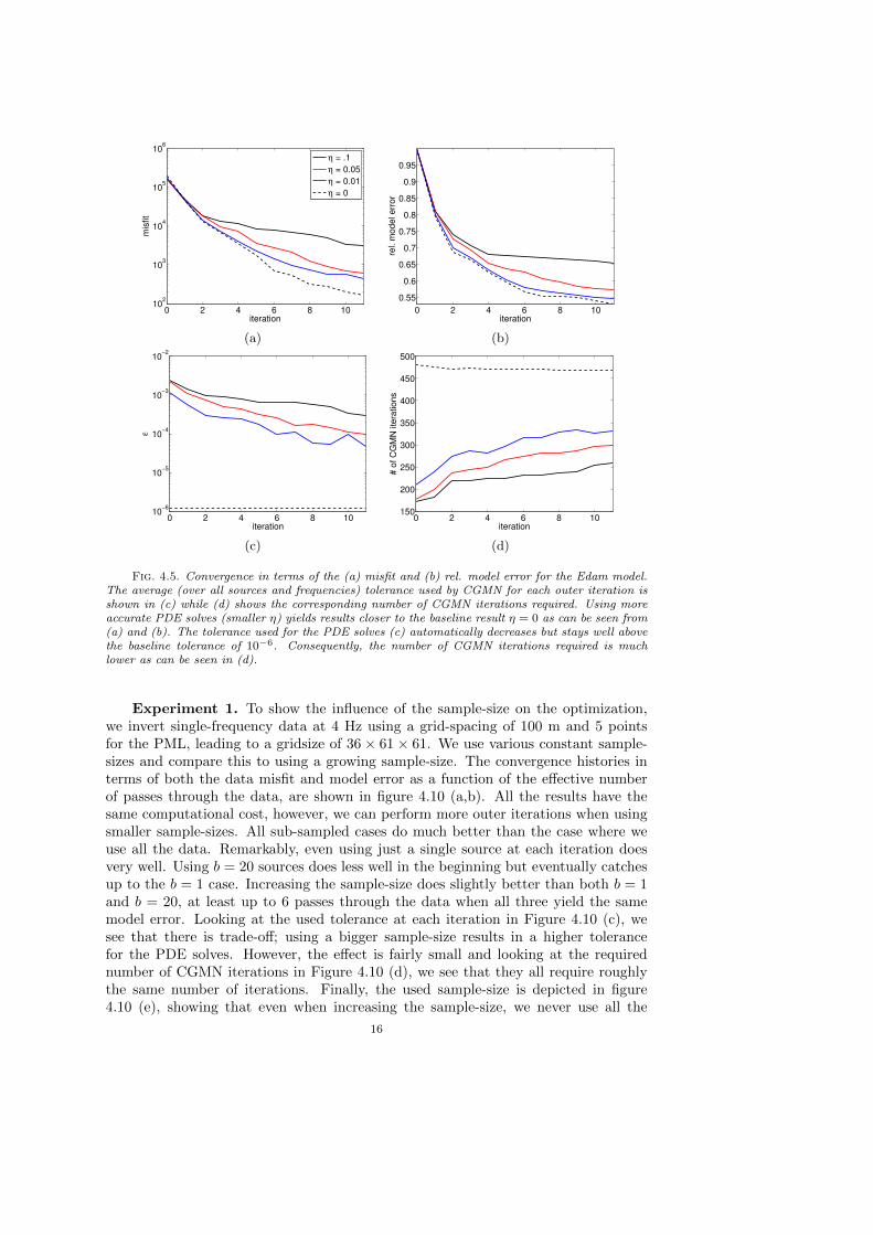
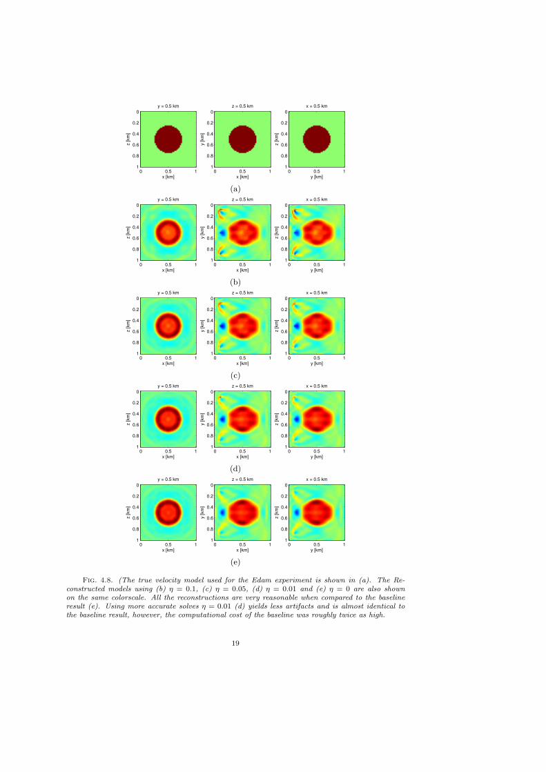
For the inversion we use all sources and frequencies simultaneously and conductthree experiments using η = {0.1, 0.05, 0.01} and compare these to a baseline resultobtained using very accurate PDE solves (η = 0). The data-misfit at each iteration isshown in figure 4.5 (a), the relative model error is shown in figure 4.5 (b), the toleranceused for the PDE solves is shown in figure 4.5 (c), and the number of CGMN iterationsrequired to reach that tolerance is shown in figure 4.5 (d). The tolerance graduallydecreases (automatically), confirming that very accurate PDE solves are not neededin the early stages of the inversion. Moreover, the results for η = 0.01 are nearlyidentical to those for η = 0, while the former was roughly twice as cheap, as can beseen by computing the total number of CGMN iterations needed from figure 4.5 (d).The true and reconstructed models are shown in figure 4.8. All the reconstructionsare very reasonable when compared to the baseline result (figure 4.8 (e)). Using moreaccurate solves η = 0.01 (figure 4.8 (d)) yields less artifacts and is almost identical tothe baseline result, however, the computational cost of the baseline result was roughlytwice as high.
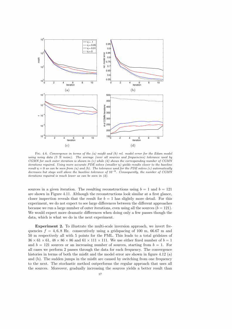
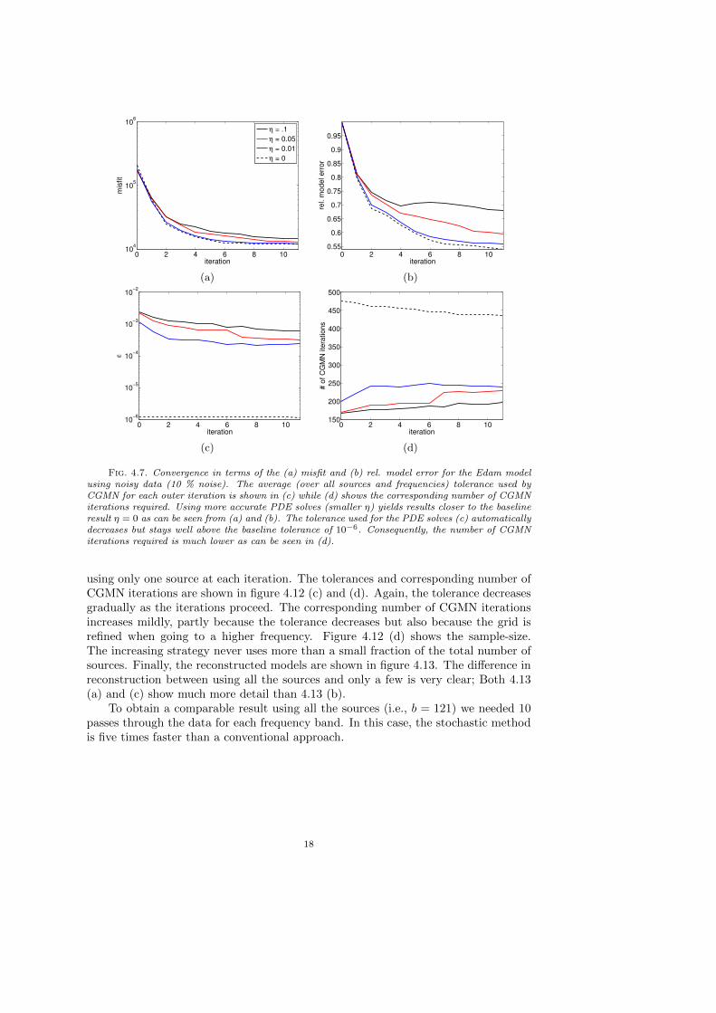
We repeat the above described experiment using data with 5% and 10% additiveGaussian noise. The convergence plots are shown in figures 4.6 and 4.7 respectively.Comparing these figures to the noiseless case (figure 4.5) we see that the method isnot affected by this moderate amount of noise.
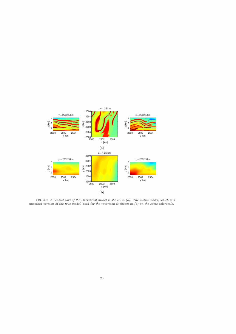
4.3. Overthrust model. We generate data using iWAVE, an open-source time-domain finite-difference code [45], for a 5 km x 5 km central part of a well-knownbenchmark model for seismic inversion (the Overthrust model) gridded with 50 mspacing. The true and initial models are shown in Figure 4.9. A total of 121 sourcesand 2601 receivers (both regularly spaced) cover the top of the model.
While significantly bigger than the previous problem, this is still a post-stampmodel compared to industry-scale problems, which easily consist of 109 gridpointsand 1000s of sources.
15
0 2 4 6 8 1010
2
103
104
105
106
iteration
mis
fit
η = .1
η = 0.05
η = 0.01
η = 0
0 2 4 6 8 10
0.55
0.6
0.65
0.7
0.75
0.8
0.85
0.9
0.95
iteration
rel. m
odel err
or
(a) (b)
0 2 4 6 8 1010
−6
10−5
10−4
10−3
10−2
iteration
ε
0 2 4 6 8 10150
200
250
300
350
400
450
500
iteration
# o
f C
GM
N ite
rations
(c) (d)
Fig. 4.5. Convergence in terms of the (a) misfit and (b) rel. model error for the Edam model.The average (over all sources and frequencies) tolerance used by CGMN for each outer iteration isshown in (c) while (d) shows the corresponding number of CGMN iterations required. Using moreaccurate PDE solves (smaller η) yields results closer to the baseline result η = 0 as can be seen from(a) and (b). The tolerance used for the PDE solves (c) automatically decreases but stays well abovethe baseline tolerance of 10−6. Consequently, the number of CGMN iterations required is muchlower as can be seen in (d).
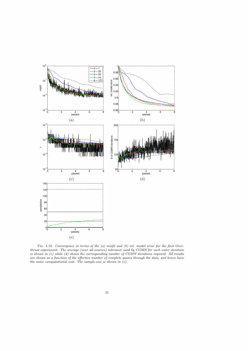
Experiment 1. To show the influence of the sample-size on the optimization,we invert single-frequency data at 4 Hz using a grid-spacing of 100 m and 5 pointsfor the PML, leading to a gridsize of 36× 61× 61. We use various constant sample-sizes and compare this to using a growing sample-size. The convergence histories interms of both the data misfit and model error as a function of the effective numberof passes through the data, are shown in figure 4.10 (a,b). All the results have thesame computational cost, however, we can perform more outer iterations when usingsmaller sample-sizes. All sub-sampled cases do much better than the case where weuse all the data. Remarkably, even using just a single source at each iteration doesvery well. Using b = 20 sources does less well in the beginning but eventually catchesup to the b = 1 case. Increasing the sample-size does slightly better than both b = 1and b = 20, at least up to 6 passes through the data when all three yield the samemodel error. Looking at the used tolerance at each iteration in Figure 4.10 (c), wesee that there is trade-off; using a bigger sample-size results in a higher tolerancefor the PDE solves. However, the effect is fairly small and looking at the requirednumber of CGMN iterations in Figure 4.10 (d), we see that they all require roughlythe same number of iterations. Finally, the used sample-size is depicted in figure4.10 (e), showing that even when increasing the sample-size, we never use all the
16
0 2 4 6 8 1010
3
104
105
106
iteration
mis
fit
η = .1
η = 0.05
η = 0.01
η = 0
0 2 4 6 8 10
0.55
0.6
0.65
0.7
0.75
0.8
0.85
0.9
0.95
iteration
rel. m
odel err
or
(a) (b)
0 2 4 6 8 1010
−6
10−5
10−4
10−3
10−2
iteration
ε
0 2 4 6 8 10150
200
250
300
350
400
450
500
iteration
# o
f C
GM
N ite
rations
(c) (d)
Fig. 4.6. Convergence in terms of the (a) misfit and (b) rel. model error for the Edam modelusing noisy data (5 % noise). The average (over all sources and frequencies) tolerance used byCGMN for each outer iteration is shown in (c) while (d) shows the corresponding number of CGMNiterations required. Using more accurate PDE solves (smaller η) yields results closer to the baselineresult η = 0 as can be seen from (a) and (b). The tolerance used for the PDE solves (c) automaticallydecreases but stays well above the baseline tolerance of 10−6. Consequently, the number of CGMNiterations required is much lower as can be seen in (d).
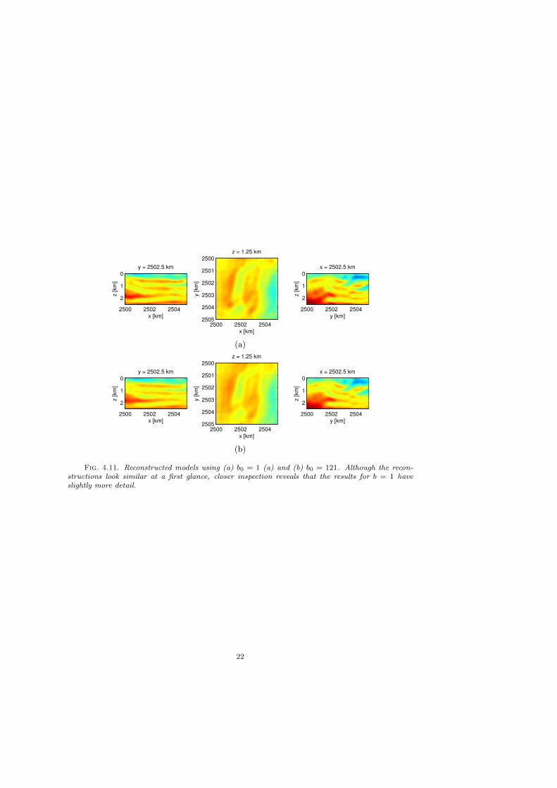
sources in a given iteration. The resulting reconstructions using b = 1 and b = 121are shown in Figure 4.11. Although the reconstructions look similar at a first glance,closer inspection reveals that the result for b = 1 has slightly more detail. For thisexperiment, we do not expect to see large differences between the different approachesbecause we run a large number of outer iterations, even using all the sources (b = 121).We would expect more dramatic differences when doing only a few passes though thedata, which is what we do in the next experiment.
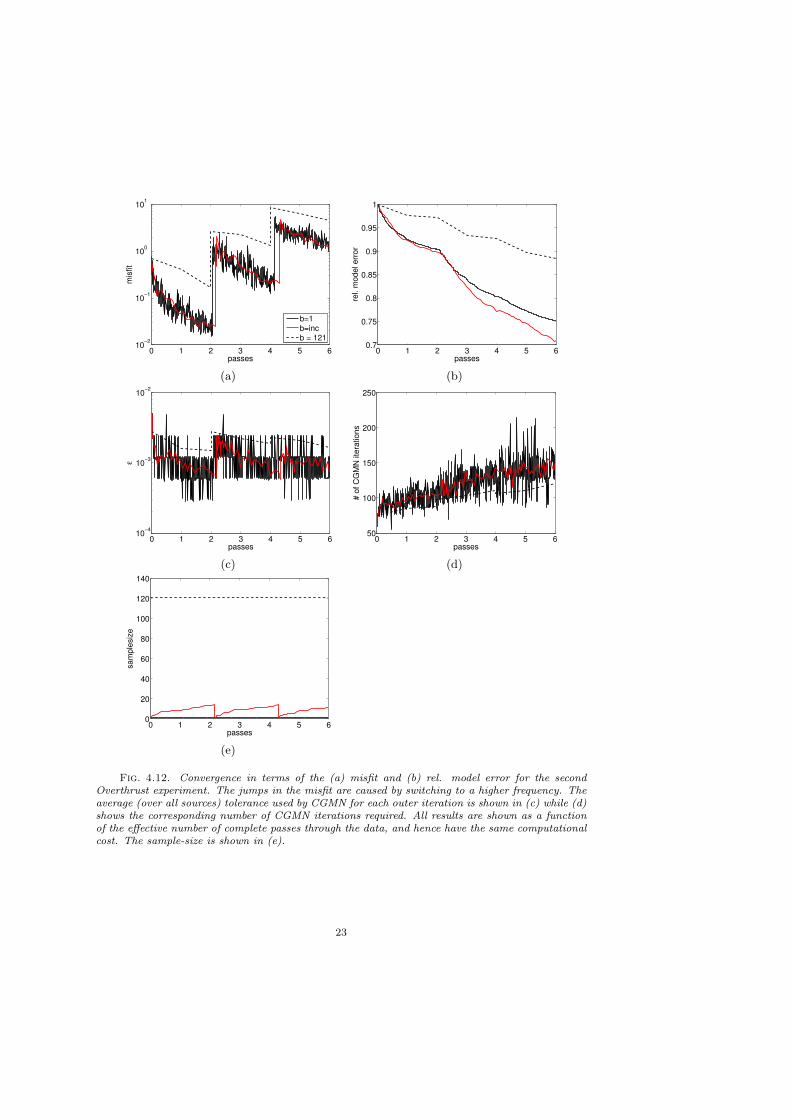
Experiment 2. To illustrate the multi-scale inversion approach, we invert fre-quencies f = 4, 6, 8 Hz. consecutively using a gridspacing of 100 m, 66.67 m and50 m respectively all with 5 points for the PML. This leads to a total gridsizes of36× 61× 61, 48× 86× 86 and 61× 111× 111. We use either fixed number of b = 1and b = 121 sources or an increasing number of sources, starting from b = 1. Forall cases we perform 2 passes through the data for each frequency. The convergencehistories in terms of both the misfit and the model error are shown in figure 4.12 (a)and (b). The sudden jumps in the misfit are caused by switching from one frequencyto the next. The stochastic method outperforms the regular approach that uses allthe sources. Moreover, gradually increasing the sources yields a better result than
17
0 2 4 6 8 1010
4
105
106
iteration
mis
fit
η = .1
η = 0.05
η = 0.01
η = 0
0 2 4 6 8 10
0.55
0.6
0.65
0.7
0.75
0.8
0.85
0.9
0.95
iteration
rel. m
odel err
or
(a) (b)
0 2 4 6 8 1010
−6
10−5
10−4
10−3
10−2
iteration
ε
0 2 4 6 8 10150
200
250
300
350
400
450
500
iteration
# o
f C
GM
N ite
rations
(c) (d)
Fig. 4.7. Convergence in terms of the (a) misfit and (b) rel. model error for the Edam modelusing noisy data (10 % noise). The average (over all sources and frequencies) tolerance used byCGMN for each outer iteration is shown in (c) while (d) shows the corresponding number of CGMNiterations required. Using more accurate PDE solves (smaller η) yields results closer to the baselineresult η = 0 as can be seen from (a) and (b). The tolerance used for the PDE solves (c) automaticallydecreases but stays well above the baseline tolerance of 10−6. Consequently, the number of CGMNiterations required is much lower as can be seen in (d).
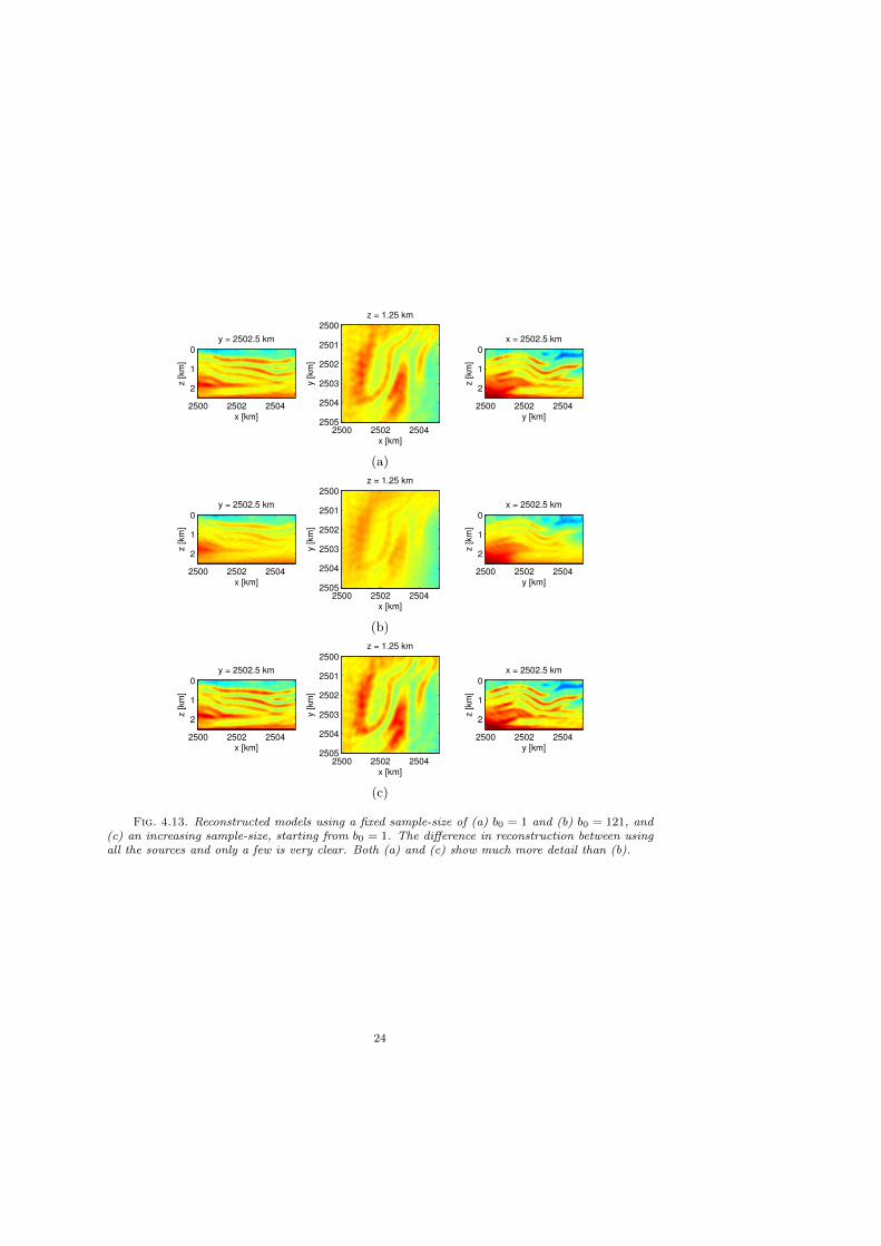
using only one source at each iteration. The tolerances and corresponding number ofCGMN iterations are shown in figure 4.12 (c) and (d). Again, the tolerance decreasesgradually as the iterations proceed. The corresponding number of CGMN iterationsincreases mildly, partly because the tolerance decreases but also because the grid isrefined when going to a higher frequency. Figure 4.12 (d) shows the sample-size.The increasing strategy never uses more than a small fraction of the total number ofsources. Finally, the reconstructed models are shown in figure 4.13. The difference inreconstruction between using all the sources and only a few is very clear; Both 4.13(a) and (c) show much more detail than 4.13 (b).
To obtain a comparable result using all the sources (i.e., b = 121) we needed 10passes through the data for each frequency band. In this case, the stochastic methodis five times faster than a conventional approach.
18
x [km]
z [km
]
y = 0.5 km
0 0.5 1
0
0.2
0.4
0.6
0.8
1
x [km]
y [km
]
z = 0.5 km
0 0.5 1
0
0.2
0.4
0.6
0.8
1
y [km]
z [km
]
x = 0.5 km
0 0.5 1
0
0.2
0.4
0.6
0.8
1
(a)
x [km]
z [km
]
y = 0.5 km
0 0.5 1
0
0.2
0.4
0.6
0.8
1
x [km]
y [km
]z = 0.5 km
0 0.5 1
0
0.2
0.4
0.6
0.8
1
y [km]z [km
]
x = 0.5 km
0 0.5 1
0
0.2
0.4
0.6
0.8
1
(b)
x [km]
z [km
]
y = 0.5 km
0 0.5 1
0
0.2
0.4
0.6
0.8
1
x [km]
y [km
]
z = 0.5 km
0 0.5 1
0
0.2
0.4
0.6
0.8
1
y [km]
z [km
]
x = 0.5 km
0 0.5 1
0
0.2
0.4
0.6
0.8
1
(c)
x [km]
z [km
]
y = 0.5 km
0 0.5 1
0
0.2
0.4
0.6
0.8
1
x [km]
y [km
]
z = 0.5 km
0 0.5 1
0
0.2
0.4
0.6
0.8
1
y [km]
z [km
]
x = 0.5 km
0 0.5 1
0
0.2
0.4
0.6
0.8
1
(d)
x [km]
z [km
]
y = 0.5 km
0 0.5 1
0
0.2
0.4
0.6
0.8
1
x [km]
y [km
]
z = 0.5 km
0 0.5 1
0
0.2
0.4
0.6
0.8
1
y [km]
z [km
]
x = 0.5 km
0 0.5 1
0
0.2
0.4
0.6
0.8
1
(e)
Fig. 4.8. (The true velocity model used for the Edam experiment is shown in (a). The Re-constructed models using (b) η = 0.1, (c) η = 0.05, (d) η = 0.01 and (e) η = 0 are also shownon the same colorscale. All the reconstructions are very reasonable when compared to the baselineresult (e). Using more accurate solves η = 0.01 (d) yields less artifacts and is almost identical tothe baseline result, however, the computational cost of the baseline was roughly twice as high.
19
x [km]
z [km
]
y = 2502.5 km
2500 2502 2504
0
1
2
x [km]
y [km
]
z = 1.25 km
2500 2502 2504
2500
2501
2502
2503
2504
2505y [km]
z [km
]
x = 2502.5 km
2500 2502 2504
0
1
2
(a)
x [km]
z [km
]
y = 2502.5 km
2500 2502 2504
0
1
2
x [km]
y [km
]
z = 1.25 km
2500 2502 2504
2500
2501
2502
2503
2504
2505y [km]
z [km
]
x = 2502.5 km
2500 2502 2504
0
1
2
(b)
Fig. 4.9. A central part of the Overthrust model is shown in (a). The initial model, which is asmoothed version of the true model, used for the inversion is shown in (b) on the same colorscale.
20
0 2 4 6 810
−3
10−2
10−1
100
passes
mis
fit
b = 1
b = 20
b = 50
b = inc
b = 121
0 2 4 6 80.86
0.88
0.9
0.92
0.94
0.96
0.98
1
passes
rel. m
odel err
or
(a) (b)
0 2 4 6 810
−5
10−4
10−3
10−2
passes
ε
0 2 4 6 850
100
150
200
passes
# o
f C
GM
N ite
rations
(c) (d)
0 2 4 6 80
20
40
60
80
100
120
140
passes
sam
ple
siz
e
(e)
Fig. 4.10. Convergence in terms of the (a) misfit and (b) rel. model error for the first Over-thrust experiment. The average (over all sources) tolerance used by CGMN for each outer iterationis shown in (c) while (d) shows the corresponding number of CGMN iterations required. All resultsare shown as a function of the effective number of complete passes through the data, and hence havethe same computational cost. The sample-size is shown in (e).
21
x [km]
z [km
]
y = 2502.5 km
2500 2502 2504
0
1
2
x [km]
y [km
]
z = 1.25 km
2500 2502 2504
2500
2501
2502
2503
2504
2505y [km]
z [km
]
x = 2502.5 km
2500 2502 2504
0
1
2
(a)
x [km]
z [km
]
y = 2502.5 km
2500 2502 2504
0
1
2
x [km]
y [km
]
z = 1.25 km
2500 2502 2504
2500
2501
2502
2503
2504
2505y [km]
z [km
]
x = 2502.5 km
2500 2502 2504
0
1
2
(b)
Fig. 4.11. Reconstructed models using (a) b0 = 1 (a) and (b) b0 = 121. Although the recon-structions look similar at a first glance, closer inspection reveals that the results for b = 1 haveslightly more detail.
22
0 1 2 3 4 5 610
−2
10−1
100
101
passes
mis
fit
b=1
b=inc
b = 121
0 1 2 3 4 5 60.7
0.75
0.8
0.85
0.9
0.95
1
passesre
l. m
odel err
or
(a) (b)
0 1 2 3 4 5 610
−4
10−3
10−2
passes
ε
0 1 2 3 4 5 650
100
150
200
250
passes
# o
f C
GM
N ite
rations
(c) (d)
0 1 2 3 4 5 60
20
40
60
80
100
120
140
passes
sam
ple
siz
e
(e)
Fig. 4.12. Convergence in terms of the (a) misfit and (b) rel. model error for the secondOverthrust experiment. The jumps in the misfit are caused by switching to a higher frequency. Theaverage (over all sources) tolerance used by CGMN for each outer iteration is shown in (c) while (d)shows the corresponding number of CGMN iterations required. All results are shown as a functionof the effective number of complete passes through the data, and hence have the same computationalcost. The sample-size is shown in (e).
23
x [km]
z [km
]
y = 2502.5 km
2500 2502 2504
0
1
2
x [km]
y [km
]z = 1.25 km
2500 2502 2504
2500
2501
2502
2503
2504
2505y [km]
z [km
]
x = 2502.5 km
2500 2502 2504
0
1
2
(a)
x [km]
z [km
]
y = 2502.5 km
2500 2502 2504
0
1
2
x [km]
y [km
]
z = 1.25 km
2500 2502 2504
2500
2501
2502
2503
2504
2505y [km]
z [km
]
x = 2502.5 km
2500 2502 2504
0
1
2
(b)
x [km]
z [km
]
y = 2502.5 km
2500 2502 2504
0
1
2
x [km]
y [km
]
z = 1.25 km
2500 2502 2504
2500
2501
2502
2503
2504
2505y [km]
z [km
]
x = 2502.5 km
2500 2502 2504
0
1
2
(c)
Fig. 4.13. Reconstructed models using a fixed sample-size of (a) b0 = 1 and (b) b0 = 121, and(c) an increasing sample-size, starting from b0 = 1. The difference in reconstruction between usingall the sources and only a few is very clear. Both (a) and (c) show much more detail than (b).
24
5. Conclusions and discussion. In this paper, we outlined the challenges facedby industry to come up with a versatile and practical 3D inversion scheme that scalesto large problem sizes with many right-hand-sides. We made it clear that comingup with scalable inversion schemes is extremely challenging because of i) the needto propagate tens to hundreds of wavelenghts, leading to large computational grids(∼ 109 gridpoints), and ii) the large amount of source experiments (typically 1000s),requiring 1000s of PDE solves at each iteration of a conventional non-linear data-fitting algorithm. While industry is slowly incorporating full-waveform inversion basedon the scalar wave equation into their workflows, major challenges remain given thethe recent push towards multi-parameter inversions with vector-Helmholtz equations.
We address a number of these challenges by developing a new stochastic inversionalgorithm designed to work with small subsets of right-hand-sides and inexact PDEsolves. Our method derives from the observation that we can allow for large errors inthe gradient calculations (as compared to the full gradient computed with exact PDEsolves and all the right-hand sides) in the course of a gradient-based optimizationalgorithm, as long as these errors are gradually decreased as the algorithm converges.The errors are controlled via heuristics that automatically adapt the sample-size andaccuracy of the PDE solves.
To solve the Helmholtz equation we used the CGMN method and its parallelextension, CARP-CG. While this preconditioner may not be optimal in the sense ofrequiring only a few iterations or an iteration count that is independent of the size ofthe system, our approach has a few notable advantages that make it a very suitablecandidate for use in a scalable inversion framework, namely i) it is guaranteed toconverge and does not rely on model-specific tuning parameters that may change asthe inversion progresses, ii) the iterations are very cheap, are easily parallelized andallow for straightforward matrix-free implementation, iii) the preconditioner is genericand hence the inversion algorithm can be easily extended to multi-parameter elasticinversion using a vector Helmholtz equation. Aside from these three key advantages,the CARP-CG based preconditioner is well suited for a control of the accuracy duringthe early stages of the inversion. For instance, in our examples we never neededvery accurate solves limiting the Helmholtz solves to no more than a few hundredCGMN iterations to converge to the desired accuracy. We also found in our numericalexamples that CGMN outperforms BiCGstab and GMRES (both with an ILU(0)preconditioner) for high frequencies.
To further speed up the inversion of multi-source seismic data, we extendedCGMN to a block-iterative method that handles multiple right-hand-sides at thesame time. Numerical experiments showed that this block-iterative Helmholtz solvercan significantly speed up the convergence as long as we avoid a breakdown due toloss of orthogonality of the residuals. In our application the right-hand-sides representindividual source experiments, which are naturally independent when their physicallocations are far apart. Hence, the initial residuals are naturally orthogonal and inour numerical experiments we typically reach the desired tolerance before the resid-uals become (numerically) linearly dependent. For a more robust implementation,variable-block or deflation techniques can be used but these are beyond the scope ofthis paper. Finally, the parallel extension of the Kaczmarz-based preconditioner weused resembles an additive Schwarz approach but with the difference that convergenceis still guaranteed. Moreover, our numerical examples show that the method scaleswell and that using more domains does not critically slow down the convergence.
Aside from heuristics to adapt sample-size and accuracy as needed by the inver-
25
sion, the true contribution of this paper lies in striking a balance between speedingup the Helmholtz solves, via model-space parallelism in the form of domain decom-position, and data-space parallelism by looping over different frequencies and sourcesubsets. Striking this balance is critical because massively parallel Helmholtz solves,with their memory overhead and setup costs, would immediately saturate the largestcompute clusters for realistic full-waveform inversion problems that involve manysource experiments. Without the high level of parallelism via domain decompositions,blocks of multiple right-hand-sides, and parallelism over randomized source subsetsand frequencies, we would not be able to attain the level of parallelism required byfull-waveform inversion in an industrial setting.
We demonstrate the efficacy of our inversion framework on two relatively smallbenchmark models (132651 unknowns, 9 sources and 520251 unknowns, 121 sources)and the results are very encouraging and show the practical validity of the proposedheuristics of adaptively increasing the accuracy of the PDE solves and the sample-size. With our adaptive approach, we get competitive inversion results at a cost thatis equivalent to performing only a few iterations with all the data at full accuracy.
In summary, we developed an adaptive stochastic algorithm for seismic waveforminversion geared towards application to large-scale seismic datasets. We attain a highlevel of parallelism by iteratively inverting domain-decomposed Helmholtz systemsfor manageable numbers of blocked right-hand-sides made of randomized subsets ofsource experiments. Our approach leads to drastic accelerations as it only increasesthe sample size and accuracy of the Helmholtz solves as needed by the optimiza-tion to converge. Numerical results on small benchmark models are very promising.While scalability to industrial data-sets has not been shown, we see no fundamentaldifficulties in doing so.
Acknowledgments. The authors wish to thank Dan and Rachel Gordon andMichael Friedlander for valuable discussions, and Uri Ascher and Eldad Haber forvaluable feedback on the first draft this manuscript. Zhi Long Fang is gratefully ac-knowledged for his contribution to the parallel Matlab code. This work was in partfinancially supported by the Natural Sciences and Engineering Research Council ofCanada Discovery Grant (22R81254) and the Collaborative Research and Develop-ment Grant DNOISE II (375142-08). This research was carried out as part of theSINBAD II project with support from the following organizations: BG Group, BGP,BP, Chevron, CGG, ConocoPhillips, ION, Petrobras, PGS, Total SA, WesternGecoand Woodside.
26
REFERENCES
[1] A.Y. Aravkin, M.P. Friedlander, F.J. Herrmann, and T. van Leeuwen, Robust inver-sion, dimensionality reduction, and randomized sampling, Mathematical Programming,134 (2012), pp. 101–125.
[2] A.Y. Aravkin and T. van Leeuwen, Estimating nuisance parameters in inverse problems,Inverse Problems, 28 (2012), p. 115016.
[3] M. Arioli, I. Duff, D. Ruiz, and M. Sadkane, Block Lanczos Techniques for Accelerating theBlock Cimmino Method, SIAM Journal on Scientific Computing, 16 (1995), pp. 1478–1511.
[4] G. Biros and O. Ghattas, Inexactness issues in the Lagrange-Newton-Krylov-Schurmethod for PDE-constrained optimization, in Large-Scale PDE-Constrained Optimization,Springer, 2003, pp. 93–114.
[5] A. Bjorck and T. Elfving, Accelerated projection methods for computing pseudoinverse so-lutions of systems of linear equations, BIT, 19 (1979), pp. 145–163.
[6] C. Bunks, Multiscale seismic waveform inversion, Geophysics, 60 (1995), p. 1457.[7] R.H. Byrd, G.M. Chin, W. Neveitt, and J. Nocedal, On the Use of Stochastic Hessian In-
formation in Optimization Methods for Machine Learning, SIAM Journal on Optimization,21 (2011), pp. 977–995.
[8] H. Calandra, S. Gratton, J. Langou, X. Pinel, and X. Vasseur, Flexible Variants of BlockRestarted GMRES Methods with Application to Geophysics, SIAM Journal on ScientificComputing, 34 (2012), pp. A714–A736.
[9] B. Engquist, Sweeping Preconditioner for the Helmholtz Equation : Hierarchical Matrix Rep-resentation, Communications on pure and applied mathematics, LXIV (2011), pp. 0697–0735.
[10] I. Epanomeritakis, V. Akcelik, O. Ghattas, and J. Bielak, A Newton-CG method forlarge-scale three-dimensional elastic full-waveform seismic inversion, Inverse Problems,24 (2008), p. 034015.
[11] Y.A. Erlangga, C. Vuik, and C.W. Oosterlee, On a robust iterative method for heteroge-neous Helmholtz problems for geophysics applications, Int. J. Numer. Anal. Model. v2, 2(2005), pp. 197–208.
[12] O.G. Ernst and M.J. Gander, Why it is difficult to solve helmholtz problems with classi-cal iterative methods, in Numerical Analysis of Multiscale Problems, Ivan G. Graham,Thomas Y. Hou, Omar Lakkis, and Robert Scheichl, eds., vol. 83 of Lecture Notes inComputational Science and Engineering, Springer Berlin Heidelberg, 2012, pp. 325–363.
[13] M.P. Friedlander and M. Schmidt, Hybrid Deterministic-Stochastic Methods for Data Fit-ting, SIAM Journal on Scientific Computing, 34 (2012), pp. A1380–A1405.
[14] D. Gordon and R. Gordon, Component-averaged row projections: A robust, block-parallelscheme for sparse linear systems, SIAM J. on Scientific Computing, 27 (2005), pp. 1092–1117.
[15] , CARP-CG: A robust and efficient parallel solver for linear systems, applied to stronglyconvection dominated pdes, Parallel Computing, 36 (2010), pp. 495–515.
[16] , Parallel solution of high-frequency Helmholtz equations using high-order finite differenceschemes, Int. Conf. on the Math. and Num. aspects of waves, (2011).
[17] D. Gordon and R. Gordon, Robust and highly scalable parallel solution of the helmholtzequation with large wave numbers, Journal of Computational and Applied Mathematics,232 (2012), pp. 182–196.
[18] A. Greenbaum, Iterative methods for solving linear systems, Society for Industrial and AppliedMathematics, Philadelphia, PA, USA, 1997.
[19] E. Haber, U.M. Ascher, and D. Oldenburg, On optimization techniques for solving non-linear inverse problems, Inverse Problems, 16 (2000), pp. 1263–1280.
[20] E. Haber, M. Chung, and F.J. Herrmann, An Effective Method for Parameter Estimationwith PDE Constraints with Multiple Right-Hand Sides, SIAM Journal on Optimization,22 (2012), pp. 739–757.
[21] E. Haber and S. MacLachlan, A fast method for the solution of the Helmholtz equation,Journal of Computational Physics, 230 (2011), pp. 4403–4418.
[22] M. Heinkenschloss and D. Ridzal, An inexact trust-region SQP method with applicationsto PDE-constrained optimization, Numerical Mathematics and Advanced Applications,(2008), pp. 613–620.
[23] M. Heinkenschloss and L.N. Vicente, Analysis of Inexact Trust-Region SQP Algorithms,SIAM Journal on Optimization, 12 (2002), pp. 283–302.
[24] S. Kaczmarz, Angenaherte auflosung von systemen linearer gleichungen, Bulletin Internationalde l’Academie Polonaise des Sciences et des Lettres, 35 (1937), pp. 355–357.
27
[25] H. Knibbe, W.A. Mulder, C.W. Oosterlee, and C. Vuik, Closing the performance gapbetween an iterative frequency-domain solver and an explicit time-domain scheme for 3Dmigration on parallel architectures, Geophysics, 79 (2014).
[26] X. Li, A.Y. Aravkin, T. van Leeuwen, and F.J. Herrmann, Fast randomized full-waveforminversion with compressive sensing, Geophysics, 77 (2012), p. A13.
[27] Y. Luo and G. Schuster, Wave-equation traveltime inversion, Geophysics, 56 (1991), p. 645.[28] P.P. Moghaddam, H. Keers, F.J. Herrmann, and W.A. Mulder, A new optimization ap-
proach for source-encoding full-waveform inversion, GEOPHYSICS, 78 (2013), pp. R125–R132.
[29] A.A. Nikishin and A.Yu. Yeremin, Variable Block CG Algorithms for Solving Large SparseSymmetric Positive Definite Linear Systems on Parallel Computers, I: General IterativeScheme, SIAM Journal on Matrix Analysis and Applications, 16 (1995), p. 1135.
[30] J. Nocedal and S.J. Wright, Numerical Optimization, Springer, 2000.[31] S. Operto, J. Virieux, P. Amestoy, J.Y. L’Excellent, L. Giraud, and H.B.H. Ali, 3D
finite-difference frequency-domain modeling of visco-acoustic wave propagation using amassively parallel direct solver: A feasibility study, Geophysics, 72 (2007), p. SM195.
[32] D. Osei-Kuffuor and Y. Saad, Preconditioning Helmholtz linear systems, Applied numericalmathematics, 60 (2010), pp. 420–431.
[33] R.-E. Plessix, A review of the adjoint-state method for computing the gradient of a functionalwith geophysical applications, Geophysical Journal International, 167 (2006), pp. 495–503.
[34] R.-E. Plessix, G Chavent, and Y.-H. De Roeck, Waveform inversion of reflection seismicdata for kinematic parameters by local inversion, SIAM Journal on Scientific Computing,20 (1999), pp. 1033–1052.
[35] J. Poulson, B. Engquist, S. Fomel, S. Li, and L. Ying, A parallel sweeping preconditionerfor high frequency heterogeneous 3D Helmholtz equations, Tech. Report 1204.0111, arXiv,Mar. 2012.
[36] G.R. Pratt, C. Shin, and G.J. Hicks, Gauss-Newton and full Newton methods in frequency-space seismic waveform inversion, Geophysical Journal International, 133 (1998), pp. 341–362.
[37] R.G. Pratt, Z.M. Song, P. Williamson, and M. Warner, Two-dimensional velocity modelsfrom wide-angle seismic data by wavefield inversion, Geophysical Journal International,124 (1996), pp. 232–340.
[38] C. Riyanti, A. Kononov, Y.A. Erlangga, C. Vuik, C. Oosterlee, R.-E. Plessix, andW.A. Mulder, A parallel multigrid-based preconditioner for the 3D heterogeneous high-frequency Helmholtz equation, Journal of Computational Physics, 224 (2007), pp. 431–448.
[39] N.N. Schraudolph, Jin Yu, and S Gunter, A stochastic Quasi-Newton Method for onlineconvex optimization, Proceedings of 11th International Conference on Artificial Intelligenceand Statistics, (2007).
[40] F. Sourbier, A. Haidar, L. Giraud, H. Ben-Hadj-Ali, J. Virieux, and S. Operto, Three-dimensional parallel frequency-domain visco-acoustic wave modelling based on a hybriddirect / iterative solver, Geophysical Prospecting, 59 (2011), pp. 834–856.
[41] W.W. Symes, Layered velocity inversion: a model problem from reflection seismology, SIAMJournal on Mathematical Analysis, 22 (1991), pp. 680–716.
[42] , Reverse time migration with optimal checkpointing, GEOPHYSICS, 72 (2007),pp. SM213–SM221.
[43] , The seismic reflection inverse problem, Inverse Problems, 25 (2009), p. 123008.[44] A. Tarantola and A. Valette, Generalized nonlinear inverse problems solved using the least
squares criterion, Reviews of Geophysics and Space Physics, 20 (1982), pp. 129–232.[45] I.S. Terentyev, T Vdovina, W.W. Symes, X. Wang, and D. Sun, IWAVE: a framework for
wave simulation.[46] K. van den Doel and U.M. Ascher, Adaptive and Stochastic Algorithms for Electrical
Impedance Tomography and DC Resistivity Problems with Piecewise Constant Solutionsand Many Measurements, SIAM Journal on Scientific Computing, 34 (2012), pp. A185–A205.
[47] T. van Leeuwen, Fourier analysis of the CGMN method for solving the Helmholtz equation,Tech. Report 1210.2644, arXiv, Oct. 2012.
[48] T. van Leeuwen, A.Y. Aravkin, and F.J. Herrmann, Seismic Waveform Inversion byStochastic Optimization, International Journal of Geophysics, (2011), pp. 1–18.
[49] T. van Leeuwen and F.J. Herrmann, Fast waveform inversion without source-encoding,Geophysical Prospecting, (2012), pp. no–no.
[50] , Mitigating local minima in full-waveform inversion by expanding the search space,Geophysical Journal International, 195 (2013), pp. 661–667.
28
[51] T. van Leeuwen and W.A. Mulder, A comparison of seismic velocity inversion methods forlayered acoustics, Inverse Problems, 26 (2010), p. 015008.
[52] , A correlation-based misfit criterion for wave-equation traveltime tomography, Geophys-ical Journal International, 182 (2010), pp. 1383–1394.
[53] J. Virieux and S. Operto, An overview of full-waveform inversion in exploration geophysics,Geophysics, 74 (2009), pp. WCC1–WCC26.
[54] S. Wang, M.V. de Hoop, and J. Xia, On 3D modeling of seismic wave propagation via astructured parallel multifrontal direct Helmholtz solver, Geophysical Prospecting, 59 (2011),pp. 857–873.
[55] J. Young and D. Ridzal, An Application of Random Projection to Parameter Estimationin Partial Differential Equations, SIAM Journal on Scientific Computing, 34 (2012),pp. A2344–A2365.
29