3D joint inversion of seismic traveltime and gravity data: a case study Dengguo Zhou

*1, Daniel R.H. O’Connell

2, Weizhong Wang

1 , Jie Zhang

1, 1GeoTomo LLC, 2Fugro Consultants

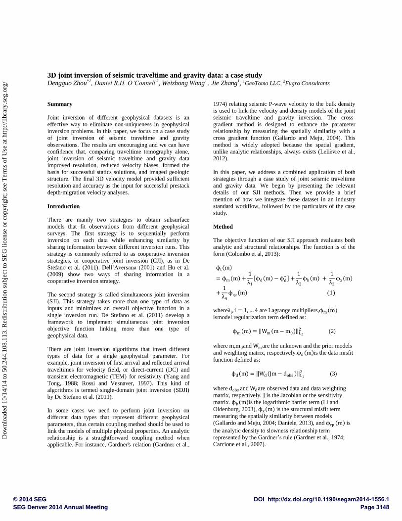
Summary Joint inversion of different geophysical datasets is an effective way to eliminate non-uniqueness in geophysical inversion problems. In this paper, we focus on a case study of joint inversion of seismic traveltime and gravity

observations. The results are encouraging and we can have confidence that, comparing traveltime tomography alone, joint inversion of seismic traveltime and gravity data improved resolution, reduced velocity biases, formed the basis for successful statics solutions, and imaged geologic structure. The final 3D velocity model provided sufficient resolution and accuracy as the input for successful prestack depth-migration velocity analyses.

Introduction There are mainly two strategies to obtain subsurface models that fit observations from different geophysical surveys. The first strategy is to sequentially perform inversion on each data while enhancing similarity by sharing information between different inversion runs. This

strategy is commonly referred to as cooperative inversion strategies, or cooperative joint inversion (CJI), as in De Stefano et al. (2011). Dell’Aversana (2001) and Hu et al. (2009) show two ways of sharing information in a cooperative inversion strategy. The second strategy is called simultaneous joint inversion (SJI). This strategy takes more than one type of data as inputs and minimizes an overall objective function in a

single inversion run. De Stefano et al. (2011) develop a framework to implement simultaneous joint inversion objective function linking more than one type of geophysical data. There are joint inversion algorithms that invert different types of data for a single geophysical parameter. For example, joint inversion of first arrival and reflected arrival

traveltimes for velocity field, or direct-current (DC) and transient electromagnetic (TEM) for resistivity (Yang and Tong, 1988; Rossi and Vesnaver, 1997). This kind of algorithms is termed single-domain joint inversion (SDJI) by De Stefano et al. (2011). In some cases we need to perform joint inversion on different data types that represent different geophysical

parameters, thus certain coupling method should be used to link the models of multiple physical properties. An analytic relationship is a straightforward coupling method when applicable. For instance, Gardner's relation (Gardner et al.,

1974) relating seismic P-wave velocity to the bulk density is used to link the velocity and density models of the joint seismic traveltime and gravity inversion. The cross-gradient method is designed to enhance the parameter relationship by measuring the spatially similarity with a cross gradient function (Gallardo and Meju, 2004). This

method is widely adopted because the spatial gradient, unlike analytic relationships, always exists (Lelièvre et al., 2012). In this paper, we address a combined application of both strategies through a case study of joint seismic traveltime and gravity data. We begin by presenting the relevant details of our SJI methods. Then we provide a brief

mention of how we integrate these dataset in an industry standard workflow, followed by the particulars of the case study.

Method

The objective function of our SJI approach evaluates both analytic and structural relationships. The function is of the

form (Colombo et al, 2013):

ϕt m

= ϕm m +1

λ1

ϕd m − ϕd∗ +

1

λ2ϕb m +

1

λ3ϕx m

+1

λ4ϕrp m (1)

whereλi , i = 1, … 4 are Lagrange multipliers,ϕm m ismodel regularization term defined as:

ϕm m = Wm m − m0 L2

2 (2)

where m,m0and Wmare the unknown and the prior models

and weighting matrix, respectively.ϕd m is the data misfit

function defined as:

ϕd m = Wd Jm − dobs L2

2 (3)

where dobs and Wdare observed data and data weighting

matrix, respectively. J is the Jacobian or the sensitivity

matrix. ϕb m is the logarithmic barrier term (Li and

Oldenburg, 2003), ϕx m is the structural misfit term

measuring the spatially similarity between models (Gallardo and Meju, 2004; Daniele, 2013), and ϕrp m is

the analytic density to slowness relationship term represented by the Gardner’s rule (Gardner et al., 1974; Carcione et al., 2007).

Page 3148SEG Denver 2014 Annual MeetingDOI http://dx.doi.org/10.1190/segam2014-1556.1© 2014 SEG

Dow

nloa

ded

10/1

4/14

to 5

0.24

4.10

8.11

3. R

edis

trib

utio

n su

bjec

t to

SEG

lice

nse

or c

opyr

ight

; see

Ter

ms

of U

se a

t http

://lib

rary

.seg

.org

/

3D joint inversion of seismic traveltime and gravity data: a case study

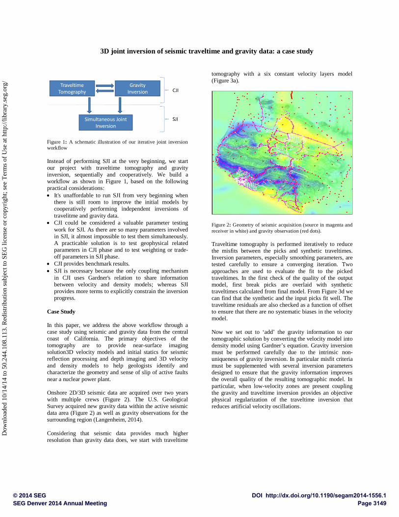
Figure 1: A schematic illustration of our iterative joint inversion

workflow Instead of performing SJI at the very beginning, we start our project with traveltime tomography and gravity inversion, sequentially and cooperatively. We build a workflow as shown in Figure 1, based on the following practical considerations:

It's unaffordable to run SJI from very beginning when there is still room to improve the initial models by cooperatively performing independent inversions of

travelitme and gravity data.

CJI could be considered a valuable parameter testing

work for SJI. As there are so many parameters involved in SJI, it almost impossible to test them simultaneously. A practicable solution is to test geophysical related parameters in CJI phase and to test weighting or trade-off parameters in SJI phase.

CJI provides benchmark results.

SJI is necessary because the only coupling mechanism

in CJI uses Gardner's relation to share information between velocity and density models; whereas SJI provides more terms to explicitly constrain the inversion progress.

Case Study

In this paper, we address the above workflow through a case study using seismic and gravity data from the central coast of California. The primary objectives of the tomography are to provide near-surface imaging solution3D velocity models and initial statics for seismic reflection processing and depth imaging and 3D velocity and density models to help geologists identify and characterize the geometry and sense of slip of active faults

near a nuclear power plant. Onshore 2D/3D seismic data are acquired over two years with multiple crews (Figure 2). The U.S. Geological Survey acquired new gravity data within the active seismic data area (Figure 2) as well as gravity observations for the surrounding region (Langenheim, 2014).

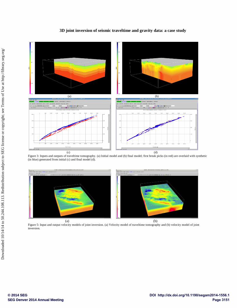
Considering that seismic data provides much higher resolution than gravity data does, we start with traveltime

tomography with a six constant velocity layers model (Figure 3a).

Figure 2: Geometry of seismic acquisition (source in magenta and

receiver in white) and gravity observation (red dots). Traveltime tomography is performed iteratively to reduce the misfits between the picks and synthetic traveltimes. Inversion parameters, especially smoothing parameters, are tested carefully to ensure a converging iteration. Two

approaches are used to evaluate the fit to the picked traveltimes. In the first check of the quality of the output model, first break picks are overlaid with synthetic traveltimes calculated from final model. From Figure 3d we can find that the synthetic and the input picks fit well. The traveltime residuals are also checked as a function of offset to ensure that there are no systematic biases in the velocity model.

Now we set out to ‘add’ the gravity information to our tomographic solution by converting the velocity model into density model using Gardner’s equation. Gravity inversion must be performed carefully due to the intrinsic non-uniqueness of gravity inversion. In particular misfit criteria must be supplemented with several inversion parameters designed to ensure that the gravity information improves the overall quality of the resulting tomographic model. In

particular, when low-velocity zones are present coupling the gravity and traveltime inversion provides an objective physical regularization of the traveltime inversion that reduces artificial velocity oscillations.

Page 3149SEG Denver 2014 Annual MeetingDOI http://dx.doi.org/10.1190/segam2014-1556.1© 2014 SEG

Dow

nloa

ded

10/1

4/14

to 5

0.24

4.10

8.11

3. R

edis

trib

utio

n su

bjec

t to

SEG

lice

nse

or c

opyr

ight

; see

Ter

ms

of U

se a

t http

://lib

rary

.seg

.org

/

3D joint inversion of seismic traveltime and gravity data: a case study

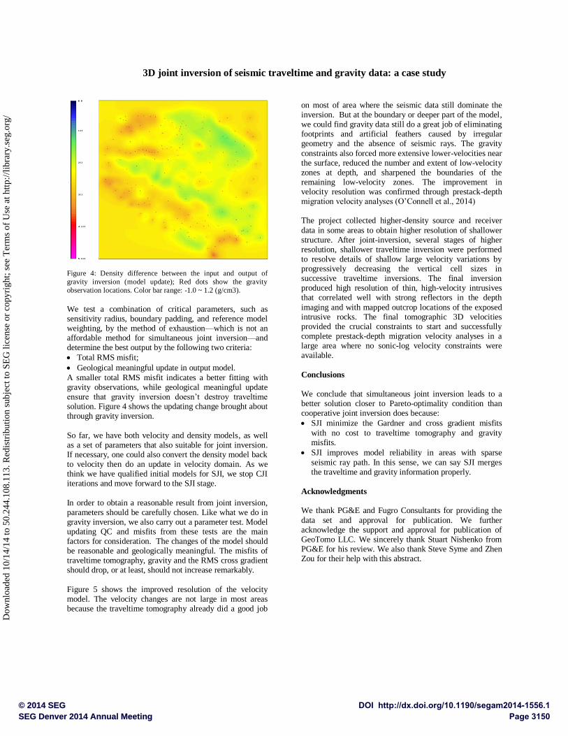
Figure 4: Density difference between the input and output of

gravity inversion (model update); Red dots show the gravity

observation locations. Color bar range: -1.0 ~ 1.2 (g/cm3). We test a combination of critical parameters, such as sensitivity radius, boundary padding, and reference model weighting, by the method of exhaustion—which is not an affordable method for simultaneous joint inversion—and determine the best output by the following two criteria:

Total RMS misfit;

Geological meaningful update in output model.

A smaller total RMS misfit indicates a better fitting with gravity observations, while geological meaningful update ensure that gravity inversion doesn’t destroy traveltime solution. Figure 4 shows the updating change brought about through gravity inversion.

So far, we have both velocity and density models, as well as a set of parameters that also suitable for joint inversion. If necessary, one could also convert the density model back to velocity then do an update in velocity domain. As we think we have qualified initial models for SJI, we stop CJI iterations and move forward to the SJI stage.

In order to obtain a reasonable result from joint inversion, parameters should be carefully chosen. Like what we do in gravity inversion, we also carry out a parameter test. Model updating QC and misfits from these tests are the main factors for consideration. The changes of the model should be reasonable and geologically meaningful. The misfits of traveltime tomography, gravity and the RMS cross gradient should drop, or at least, should not increase remarkably.

Figure 5 shows the improved resolution of the velocity model. The velocity changes are not large in most areas because the traveltime tomography already did a good job

on most of area where the seismic data still dominate the inversion. But at the boundary or deeper part of the model, we could find gravity data still do a great job of eliminating footprints and artificial feathers caused by irregular geometry and the absence of seismic rays. The gravity

constraints also forced more extensive lower-velocities near the surface, reduced the number and extent of low-velocity zones at depth, and sharpened the boundaries of the remaining low-velocity zones. The improvement in velocity resolution was confirmed through prestack-depth migration velocity analyses (O’Connell et al., 2014) The project collected higher-density source and receiver

data in some areas to obtain higher resolution of shallower structure. After joint-inversion, several stages of higher resolution, shallower traveltime inversion were performed to resolve details of shallow large velocity variations by progressively decreasing the vertical cell sizes in successive traveltime inversions. The final inversion produced high resolution of thin, high-velocity intrusives that correlated well with strong reflectors in the depth

imaging and with mapped outcrop locations of the exposed intrusive rocks. The final tomographic 3D velocities provided the crucial constraints to start and successfully complete prestack-depth migration velocity analyses in a large area where no sonic-log velocity constraints were available.

Conclusions

We conclude that simultaneous joint inversion leads to a better solution closer to Pareto-optimality condition than cooperative joint inversion does because:

SJI minimize the Gardner and cross gradient misfits

with no cost to traveltime tomography and gravity misfits.

SJI improves model reliability in areas with sparse

seismic ray path. In this sense, we can say SJI merges the traveltime and gravity information properly.

Acknowledgments We thank PG&E and Fugro Consultants for providing the

data set and approval for publication. We further acknowledge the support and approval for publication of GeoTomo LLC. We sincerely thank Stuart Nishenko from PG&E for his review. We also thank Steve Syme and Zhen Zou for their help with this abstract.

Page 3150SEG Denver 2014 Annual MeetingDOI http://dx.doi.org/10.1190/segam2014-1556.1© 2014 SEG

Dow

nloa

ded

10/1

4/14

to 5

0.24

4.10

8.11

3. R

edis

trib

utio

n su

bjec

t to

SEG

lice

nse

or c

opyr

ight

; see

Ter

ms

of U

se a

t http

://lib

rary

.seg

.org

/

3D joint inversion of seismic traveltime and gravity data: a case study

(a) (b)

(c) (d)

Figure 3: Inputs and outputs of traveltime tomography. (a) Initial model and (b) final model; first break picks (in red) are overlaid with synthetic

(in blue) generated from initial (c) and final model (d).

(a) (b)

Figure 5: Input and output velocity models of joint inversion. (a) Velocity model of traveltime tomography and (b) velocity model of joint

inversion.

Page 3151SEG Denver 2014 Annual MeetingDOI http://dx.doi.org/10.1190/segam2014-1556.1© 2014 SEG

Dow

nloa

ded

10/1

4/14

to 5

0.24

4.10

8.11

3. R

edis

trib

utio

n su

bjec

t to

SEG

lice

nse

or c

opyr

ight

; see

Ter

ms

of U

se a

t http

://lib

rary

.seg

.org

/

http://dx.doi.org/10.1190/segam2014-1556.1 EDITED REFERENCES Note: This reference list is a copy-edited version of the reference list submitted by the author. Reference lists for the 2014 SEG Technical Program Expanded Abstracts have been copy edited so that references provided with the online metadata for each paper will achieve a high degree of linking to cited sources that appear on the Web. REFERENCES

Alvarez, G., and K. Larner, 1996, Implications of multiple suppression for AVO analysis and CMP-stacked data: 66th Annual International Meeting, SEG, Expanded Abstracts, 1518–1521.

Carcione, J. M., B. Ursin, and J. I. Nordskag, 2007, Cross-property relations between electrical conductivity and the seismic velocity of rocks : Geophysics, 72, no. 5, E193–E204, http://dx.doi.org/10.1190/1.2762224.

Colombo, D., D. Rovetta, E. Sandoval, R. E. Ley, W. Wang, and C. Liang, 2013, 3D seismic-gravity simultaneous joint inversion for near-surface velocity estimation: Presented at the 75th Annual International Conference and Exhibition, EAGE.

De Stefano, M., F. Golfré Andreasi, S. Re, M. Virgilio, and F. F. Snyder, 2011, Multiple-domain, simultaneous joint inversion of geophysical data with application to subsalt imaging: Geophysics, 76, no. 3, R69–R80, http://dx.doi.org/10.1190/1.3554652.

Dell’Aversana, P., 2001, Integration of seismic, Mt, and gravity data in a thrust belt interpretation: First Break, 19, no. 6, 335–341, http://dx.doi.org/10.1046/j.1365-2397.2001.00158.x.

Gallardo, L. A., and M. A. Meju, 2004, Joint two-dimensional DC resistivity and seismic traveltime inversion with cross-gradients constraints: Journal of Geophysical Research, 109, B3, B03311, http://dx.doi.org/10.1029/2003JB002716.

Gardner, G. H. F., L. W. Gardner, and A. R. Gregory, 1974, Formation velocity and density — The diagnostic basics for stratigraphic traps: Geophysics, 39, 770–780, http://dx.doi.org/10.1190/1.1440465.

Hu, W., A. Abubakar, and T. M. Habashy, 2009, Joint electromagnetic and seismic inversion using structural constraints: Geophysics, 74, no. 6, R99–R109, http://dx.doi.org/10.1190/1.3246586.

Langenheim, V. E., 2014, Gravity, aeromagnetic and rock-property data of the central California coast ranges: U. S. Geological Survey Open-File Report 2013–1282, http://dx.doi.org/10.3133/ofr20131282.

Lelièvre, P. G., C. G. Farquharson, and C. A. Hurich, 2012, Joint inversion of seismic traveltimes and gravity data on unstructured grids with application to mineral exploration: Geophysics, 77, no. 1, K1–K15, http://dx.doi.org/10.1190/geo2011-0154.1.

O’Connell, D.R.H., S. Nishenko, K. Brock, G. Stankovic , N. Pralica, D. Zhou, and W. Wang, 2014, Onshore depth imaging with extremely crooked 2D and irregular 3D seismic data in rugged terrain: Presented at the 84th Annual International Meeting, SEG.

Rossi, G., and A. Vesnaver, 1997, 3D imaging by adaptive joint inversion of reflected and refracted arrivals: 67th Annual International Meeting, SEG, Expanded Abstracts, 1873–1876.

Yang, C. H., and L. T. Tong, 1988, Joint inversion of DC, TEM, and MT data: Presented at the 58th Annual International Meeting, SEG.

Page 3152SEG Denver 2014 Annual MeetingDOI http://dx.doi.org/10.1190/segam2014-1556.1© 2014 SEG

Dow

nloa

ded

10/1

4/14

to 5

0.24

4.10

8.11

3. R

edis

trib

utio

n su

bjec

t to

SEG

lice

nse

or c

opyr

ight

; see

Ter

ms

of U

se a

t http

://lib

rary

.seg

.org

/