Embed Size (px)
Citation preview

3D LASER HOLOGRAPHIC INTERFEROMETRY MEASUREMENTS
by
Zhenhua Huang
A dissertation submitted in partial fulfillment of the requirements for the degree of
Doctor of Philosophy (Mechanical Engineering)
in The University of Michigan 2006
Doctoral Committee: Associate Professor Albert J. Shih, Co-Chair Professor Jun Ni, Co-Chair
Professor Elijah Kannatey-Asibu Jr Professor Jianjun Shi Adjunct Assistant Professor John Patrick Spicer

© Zhenhua Huang 2006 All rights reserved

ii
To my beloved family, especially my wife Mingmin Zhu and my daughter Cindy Huang.

iii
Acknowledgements
I would like to express my sincere gratitude to my advisors Dr. Albert Shih and
Dr. Jun Ni for their continuous guidance and education not only on my research but also
on my moral maturity. Dr. Shih and Dr. Ni spent tremendous time from their busy
schedules teaching me word by word how to write good papers and how to give good
presentations. They also coached me through many trivial details how to treat other
people well and how to be a good man. The significant efforts from Dr. Shih and Dr. Ni
to secure my financial support are highly recognized.
The kind helps from all the other committee members, Dr. Jianjun Shi, Dr. Elijah
Kannatey-Asibu Jr, and Dr. Pat Spicer, are greatly appreciated.
I am grateful to Mr. Dwight Carlson, Mr. Ron Swonger, and many other
gentlemen from Coherix Inc. for their generous and unreserved technical supports. They
not only provided me the opportunity to use their advanced equipment but also created
the environment for me to learn the in-depth knowledge about this exciting technology.
The Engineering Research Center for Reconfigurable Manufacturing Systems
directed by Professor Yoram Koren generously sponsored this research. And through the
active involvement of many activities in ERC, my academic and social skills have been
improved significantly. This precious experience in ERC will be treasured through the
rest of my life.
The advanced measurement group directed by Robert Waite in DaimlerChrysler
helped me initiate this exciting research area and provided me the access to their state-of-
the-art instruments. The CogniTens Ltd. under Eyal Mizrahi also offered a lot of
measurement help. Professor Jack Hu generously offered me the opportunities to use his
devices for my research experiments. I thank them all.

iv
My family, especially my wife Mingmin, always stood behind me throughout the
four year PhD study, no matter up or down. Without their supports, I could not make this
dissertation happen.

v
Contents
Dedication ........................................................................................................................... ii
Acknowledgements............................................................................................................ iii
List of Figures .................................................................................................................. viii
List of Tables ..................................................................................................................... xi
List of Appendices ............................................................................................................ xii
Chapter 1. Introduction ...................................................................................................... 1
1.1. Research motivations and goals.............................................................................. 1
1.2. Laser holographic interferometry for powertrain components measurement......... 3
1.3. Feasibility study of 3D optical systems for engine head measurement .................. 4
1.4. Overview of research .............................................................................................. 5
Chapter 2. Hologram Registration for 3D Precision Holographic Interferometry Measurement..................................................................................................................... 11
2.1. Introduction........................................................................................................... 11
2.2. Hologram registration ........................................................................................... 12
2.2.1. Translation..................................................................................................... 13
2.2.2. Tilt and shift correction ................................................................................. 14
2.2.3. Rotation ......................................................................................................... 16
2.2.3.1. Rotation identification ........................................................................... 17
2.2.3.2. Rotation correction................................................................................. 18
2.3. Accuracy evaluation of hologram registration...................................................... 19
2.3.1. Accuracy evaluation procedures.................................................................... 19
2.3.2. Example I -- wheel hub ................................................................................. 20
2.3.3. Example II -- engine head combustion deck surface..................................... 22
2.4. Concluding remarks .............................................................................................. 23
Chapter 3. Phase Unwrapping for Large Depth-of-Field 3D Laser Holographic Interferometry Measurement of Laterally Discontinuous Surfaces.................................. 33
3.1. Introduction........................................................................................................... 33
3.2. Region-referenced phase unwrapping................................................................... 35

vi
3.2.1. Principle........................................................................................................ 35
3.2.2. Segmentation and patching........................................................................... 36
3.3. Masking, dynamic segmentation and phase adjustment ....................................... 37
3.3.1. Phase wrap identification on boundary pixels.............................................. 38
3.3.2. Masking and recovery .................................................................................. 38
3.3.3. Dynamic segmentation ................................................................................. 39
3.3.4. Phase adjustment for thin boundary regions with phase wrap ..................... 40
3.4. Example ................................................................................................................ 43
3.4.1. Phase unwrapping results ............................................................................. 43
3.4.2. Effect of W and Wo on computational efficiency ......................................... 45
3.4.3. Convergence ................................................................................................. 45
3.5. Concluding remarks .............................................................................................. 46
Chapter 4........................................................................................................................... 57
Laser Holographic Interferometry Measurement of Cylinders......................................... 57
4.1. Introduction........................................................................................................... 57
4.2. Mathematical model.............................................................................................. 58
4.2.1. System design............................................................................................... 58
4.2.2. Mathematical deduction ............................................................................... 59
4.2.2.1. Geometric relation definition ................................................................ 59
4.2.2.2. Format of measurement data................................................................. 60
4.2.2.3. Data conversion .................................................................................... 61
4.2.3. Cylindricity evaluation .................................................................................. 64
4.2.4. Registration adjustment ................................................................................ 68
4.3. Calibrations ........................................................................................................... 69
4.4. Examples............................................................................................................... 69
4.4.1. Simulations ................................................................................................... 70
4.4.1.1. Cylindricity measurement ..................................................................... 70
4.4.1.2. Calibration............................................................................................. 71
4.4.1.3. Error analysis ........................................................................................ 72
4.4.2. Experiment ................................................................................................... 74
4.4.2.1. System configurations........................................................................... 74
4.4.2.2. Adjustments .......................................................................................... 75
4.4.2.3. Measurement results ............................................................................. 75

vii
4.4.2.4. Processing ............................................................................................. 76
4.5. Concluding remarks ............................................................................................... 78
Chapter 5. Conclusions and Future Work........................................................................ 92
5.1. Conclusions........................................................................................................... 92
5.2. Future work........................................................................................................... 93
5.2.1. Performance improvement of cylindricity measurement ............................. 94
5.2.2. Error analysis of geometrical form evaluation for high definition measurements .......................................................................................................... 95
Appendices........................................................................................................................ 97
References....................................................................................................................... 139

viii
List of Figures
Fig. 1.1. Examples of automotive powertrain and wheel assembly components: (a) engine head, (b) automatic transmission valve body, (c) wheel hub, and (d) wheel rotor............. 8
Fig. 1.2. Measurement size and tolerance requirement for automotive components. [1]... 9
Fig. 1.3. Top view of a V6 engine head combustion deck surface. ................................. 10
Fig. 1.4. Flatness measurement results by: (a) Zeiss CMM, model UPMC CARAT 850/1200 with a scanning probe, (b) laser holographic interferometer Coherix Shapix 1000, and (c) stereovision system CogniTens Optigo 200. .............................................. 10
Fig. 2.1. Measurement regions and variables used for hologram registration: (a) Measurement A and (b) Measurement B. In this research, W = 1024, p = 0.293 mm, and pW = 300 mm.................................................................................................................... 25
Fig. 2.2. Wheel hub: (a) isometric view, (b) top view, and (c) close-up view of the dent marked in solid rectangle in (b). ....................................................................................... 26
Fig. 2.3. Measured holograms of the wheel hub: (a) intensity and (b) phase of Measurements A and B..................................................................................................... 27
Fig. 2.4. Correlation matrix C of Measurements A and B of the wheel hub. .................. 28
Fig. 2.5. Registered hologram of the wheel hub: (a) phase and (b) intensity. ................. 29
Fig. 2.6. 3D profile measurement of the wheel hub: (a) registered measurement hm(i, j) and (b) standard measurement hs(i, j). .............................................................................. 30
Fig. 2.7. Difference between hs(i, j) and hm(i, j) of the wheel hub. ................................. 30
Fig. 2.8. Effect of the area of the overlapped region on the error erms. ............................ 31
Fig. 2.9. Overview of a V6 engine head combustion deck surface. ................................ 31
Fig. 2.10. 3D profile of the engine head combustion deck surface: (a) registered measurement and (b) CMM measurement........................................................................ 32
Fig. 3.1. Artificially created phase map: (a) 3D true phase map without phase wrap and (b) 3D wrapped phase map. .............................................................................................. 48
Fig. 3.2. The automatic transmission valve body: (a) isometric view and (b) top view.. 49
Fig. 3.3. Detection of phase wrap at pixel (i, j): (a) surrounding four pixels and (b) reference region surrounding the pixel. ............................................................................ 50
Fig. 3.4. Measured phase map with phase wrap for the automatic transmission valve body................................................................................................................................... 51

ix
Fig. 3.5. Close-up view of the region S1 in Fig. 3.4 as an example of the boundary pixels with decreased noise robustness in the detection of phase wrap: (a) before phase unwrapping, (b) after phase unwrapping and before recovery, and (c) after phase unwrapping and recovery.................................................................................................. 52
Fig. 3.6. Segmentation: (a) static segmentation of the region S2 in Fig. 3.4, (b) close-up view of the region S4 in Fig. 3.6(a), and (c) dynamic segmentation of the region S2 in Fig. 3.4...................................................................................................................................... 53
Fig. 3.7. Definition of the boundary width pm: (a) two boundary regions and (b) the condition with pixels on the top side close to the left side of the segment....................... 54
Fig. 3.8. Example of the dynamic segmentation of region S3 in Fig. 3.4 (W = 50, Wo = 20, and T = 6 pixels). .............................................................................................................. 55
Fig. 3.9. Phase unwrapping of the automatic transmission valve body: (a) unwrapped phase map without adjustment, (b) close-up view of the region S5 in (a), (c) close-up view of the region S6 in (a), (d) unwrapped phase map after adjustment, (e) close-up view of the region S΄5 in (d) after adjustment, and (f) close-up view of the region S΄6 in (d) after adjustment................................................................................................................. 56
Fig. 4.1. Conceptual system design of the laser holographic interferometry system: (a) flat object measurement and (b) cylindricity measurement.............................................. 81
Fig. 4.2. 3D illustration of the geometric relations in the mathematical model for the cylindricity measurement with the laser holographic interferometry system................... 82
Fig. 4.3. 3D illustration of four simulated laser holographic interferometry measurements of the cylinder with O0 = (0, 0, 0.5) mm, D0 = (0, 1, 0), O2 = (0, 0, –1) mm, D2 = (0.0995, 0.9950, 0), R = 12.5 mm, and S = 12 mm (O1 = (0, 0, 1) mm and D1 = (0, 0.9988, 0.0499) at the 0º angular position of the cylinder): (a) at 0º angular position, (b) at 90º angular position, (c) at the angular position of 180º, and (d) at the angular position of 270º of the cylinder. ............................................................................................................................ 83
Fig. 4.4. Generated cylinder surface profile from the simulated data (cylindricity = 7.9×10⁻⁷ mm). ................................................................................................................... 84
Fig. 4.5. The cylindricity measurement error distribution simulated by the Monte Carlo method............................................................................................................................... 85
Fig. 4.6. System configurations of the cylindricity measurement. .................................. 86
Fig. 4.7. Height measurement of the master cylinder at the angular position of 333.140º: (a) 2D color map, (b) height profile along Line1 from left to right in (a), and (c) height profile along Line 2 from top to bottom in (a).................................................................. 87
Fig. 4.8. Height measurement of the master cylinder at the angular position of 62.227º: (a) 2D color map, (b) height profile along the Line 1 from left to right in (a), and (c) height profile along the Line 2 from top to bottom in (a). ........................................................... 88
Fig. 4.9. Height measurement of the master cylinder at the angular position of 149.988º: (a) 2D color map, (b) height profile along the Line 1 from left to right in (a), and (c) height profile along the Line 2 from top to bottom in (a). ................................................ 89
x
Fig. 4.10. Height measurement of the master cylinder at the angular position of 244.377º: (a) 2D color map, (b) height profile along the Line 1 from left to right in (a), and (c) height profile along the Line 2 from top to bottom in (a). ................................................ 90
Fig. 4.11. 3D illustration of the final estimation of the master cylinder.......................... 91
Fig. 5.1. Master cylinder with negligible cylindricity errors and precisely rectified grooves.............................................................................................................................. 96
Fig. B.1. Plane light wave distribution in space at a time spot. [5] ............................... 114
Fig. B.2. Diagram of the laser holographic interferometer: (a) configuration of the machine and (b) scheme of the optical measurement unit in (a). ................................... 115
Fig. B.3. Optical configurations of the laser holographic interferometer under research.......................................................................................................................................... 116
Fig. B.4. Valve body surface flatness measurement by the laser holographic interferometer.................................................................................................................. 116
Fig. B.5. Step gage for performance evaluation: (a) overview and (b) CAD model. .... 117
Fig. B.6. Target value measurement of the step heights by Taylor Hobson contact profilometer..................................................................................................................... 117
Fig. B.7. 3D profile of the step gage measured by the laser holographic interferometer.......................................................................................................................................... 118
Fig. B.8. An automotive automatic transmission valve body for performance evaluation.......................................................................................................................................... 119
Fig. B.9. 3D profile of the automotive automatic transmission valve body measured by the laser holographic interferometry............................................................................... 120
Fig. C.1. Geometric form evaluation based on the measurement data with the part and measurement variations. ................................................................................................. 136
Fig. C.2. Simulated part variation of profile 4 without measurement errors: (a) 3D profile and (b) histogram of height distribution. ........................................................................ 136
Fig. C.3. Simulated part variation of profile 1 without measurement errors: (a) 3D profile and (b) histogram of height distribution. ........................................................................ 136
Fig. C.4. Simulated part variation of profile 2 without measurement errors: (a) 3D profile and (b) histogram of height distribution. ........................................................................ 137
Fig. C.5. Simulated part variation of profile 3 without measurement errors: (a) 3D profile and (b) histogram of height distribution. ........................................................................ 137
Fig. C.6. Simulated part variation of profile 5 without measurement errors: (a) 3D profile and (b) histogram of height distribution. ........................................................................ 138

xi
List of Tables
Table 3.1. Computational time for phase unwrapping of the automatic transmission valve body example (892 x 842 pixels)...................................................................................... 47
Table 3.2. Minimum Wo for phase unwrapping without divergence in the automatic transmission valve body example. .................................................................................... 47
Table 4.1. The cylindricity measurement error due to the parameter estimation ............ 80
Table B.1. Plane distance measurements of the step gage by the laser holographic interferometer.................................................................................................................. 112
Table B.2. Gage R&R evaluation of the laser holographic interferometer. .................. 113
Table C.1. Standard deviation of reference plane coefficients for flatness evaluation.. 134
Table C.2. Flatness evaluation error analysis of different methods............................... 135

xii
List of Appendices
Appendix A. Comparison Matrix of Six 3D Measurement Systems …………………98
Appendix B. Laser Holographic Interferometry and Performance Evaluation …………99
Appendix C. Flatness Evaluation for High Definition Measurements…………………121

1
Chapter 1
Introduction
1.1. Research motivations and goals
Automotive manufacturers are continually challenged by the needs to improve
product quality and reduce warranty cost. Effective measurement methods are required
to assure the precision and accuracy of component manufacturing, assembly, and testing.
For automobile bodies and sub-assemblies, the optical measurement technologies have
revolutionized the dimensional quality monitoring and control in the past two decades.
The optical measurement systems enable the in-line, 100% inspection and use of
advanced statistical analysis methods for root cause diagnostics. Such success has not yet
been realized in the automotive powertrain and wheel assembly.
The automotive powertrain, which includes the engine, engine accessories,
transmissions, differentials, and axles, generates and transmits powers to the wheel
assembly. Powertrain and wheel assembly components have more stringent dimensional
and geometrical form tolerances compared with body parts to meet the performance
requirements. Five examples are presented in Fig. 1.1 to illustrate the powertrain and
wheel assembly components. Typical tolerance specifications are discussed as following.
A typical V6 internal combustion engine head is shown in Fig. 1.1(a). The
combustion deck surface on the engine head is a representative feature for precision
powertrain components. The flatness specifications of this combustion deck surface are
150 µm along the 400 mm length, 100 µm across the 250 mm width, and 25 µm over any
25 mm x 25 mm surface area. Fig. 1.1(b) shows a hydraulic valve body for the automatic
transmission. The part has the flatness specifications of 50 µm over the 200 mm x 100

2
mm surface and 25 µm across any 80 mm line. The wheel hub, as shown in Fig. 1.1(c),
transmits power from the axle to wheel and supports the vehicle. The flatness
specification of the hub surface, as marked by A, is from 30 to 50 µm. Figure 1.1(d)
shows a rotor for disk brake. The surface, as marked by B on the rotor in Fig. 1.1(d),
contacts the surface A on the hub in the wheel assembly. The brake pads contact the
surface, marked by C on the rotor in Fig. 1.1(d). The runout specifications of surface C
relative to the datum surface A of the rotor is usually 50 µm or less. This specification is
critical to reduce the vehicle noise, vibration, and harshness (NVH) and improve
drivability.
A Coordinate Measurement Machine (CMM) is a flexible and accurate contact-
based measurement system which has been extensively used for the inspection of
automotive powertrain components. However, CMMs are not feasible for the in-line
inspection desired by transfer line production applications due to the extended
measurement cycle time and lack of the full surface measurement capability. Some
critical regions may be neglected. This can introduce the leakage problem when the
engine head is assembled to the engine block. Further quality control and root cause
diagnostics is also difficult from the incomplete data measured by CMMs.
The 3D non-contact optical measurement technologies have been widely utilized
in quality inspection [1], reverse engineering [2], remote sensing [3], and robot guidance
[4]. In recent years, new optical hardware and software developments have further
advanced the accuracy and reduced the cost of 3D optical measurement systems. Optical
measurement systems have been successfully applied in the automotive quality control
and process diagnosis of body manufacturing and assembly.
Figure 1.2 shows the measurement size and form tolerance requirements for
different automotive components [1]. The powertrain and wheel assembly components,
marked in boxes, have the form tolerances from 10 to 100 µm in the measurement
volume less than 0.1 m3. Extensive research efforts [5-8] have been dedicated to the
applications of non-contact optical measurements for powertrain components. There is
still a gap before widespread and practical in-line utilization by industry due to the
following three reasons. First, a wide variety of surface features, surface textures and

3
finish, and surface reflectance exist for the powertrain components. This imposes a great
challenge on precision optical measurement systems. Second, the performance of optical
measurements usually depends on the environment conditions. An optical system with
good performance in laboratory may not function well due to the vibration, thermal
deviation, and environment illumination disturbance in the production line. Third, the
measurement speed needs further improvement to satisfy the in-line measurement
requirements.
This research is motivated by the lack of effective and efficient 3D non-contact
optical measurement methods for precision automotive components. The 3D µm-level
accurate optical systems, which will be capable of the in-line, full surface precision
measurement, are targeted in this research.
1.2. Laser holographic interferometry for powertrain components measurement
A wide variety of 3D optical measurement methods are available. Based on the
principles of the data extraction for 3D dimensional and geometrical form measurement,
the 3D optical measurement methods can be categorized as: stereovision [9],
interferometry [10,11], structured lighting [12,13], laser triangulation [14], Moiré fringe
[15-17], focus detection [18,19], time-of-flight [20], and laser speckle pattern sectioning
[21]. A comparison matrix of six 3D measurement systems is illustrated in Appendix A.
The laser holographic interferometry method is demonstrated to have the potential
capabilities for in-line, full surface precision measurement of powertrain and wheel
assembly components. The basic principles and characteristics of the laser holographic
interferometry methods are described as following. The system principle, configurations,
and the performance evaluation are discussed in detail in Appendix B.
Laser holographic interferometry extracts the 3D profile of an object by
identifying the phase of the light wave which is reflected from the object surface and
carries the height information of the object. The laser holographic interferometer usually
uses a beam splitter to separate the laser into two separate beams, the reference and the
carrier beams of the same wavelength. The carrier beam is directed onto the object

4
surface and the phase is modulated by the 3D object profile. The modulated carrier beam
interferes with the reference beam and generates the hologram containing the 3D profile
information of the object surface. By identifying the phase difference at each pixel in the
hologram, the 3D profile of the object can be extracted.
The laser holographic interferometry for 3D surface profile measurement has
three advantages. (1) High accuracy. Combined with phase shifting analysis,
interferometric methods can have the accuracy of 1/100 of a fringe [22]. For a typical
system, the accuracy of the height measurement can reach 0.50 µm for a 300 mm x 300
mm field of view (FOV) with the height measurement range up to 17 mm [3]. The lateral
resolution and range of phase shifting interferometric instruments depend on the CCD
pixel spacing and the magnification of the objective. (2) No shadowing or occlusion.
Shadowing occurs when the object cannot be illuminated but is visible to the sensor.
Occlusion occurs when the object is illuminated but invisible to the sensor. Either
shadowing or occlusion does not exist in the laser holographic interferometry because the
object is illuminated and viewed from the same direction. (3) No moving parts. The 3D
image of the entire field of view is generated without scanning. With all parts fixed, the
system has high reliability and repeatability.
There are three limitations for the current laser holographic interferometry method.
First, the measurement area is limited by the system FOV and no hologram registration
method is available for the measurement of part larger than the system FOV. Second, the
height measurement range is limited by the optical configurations. And the height
measurement accuracy and resolution will decrease if the height measurement range
increases using the wavelength-tuning technology. Third, difficulties are usually
expected for the precision measurement of round and more generally free-form specular
surfaces due to the large surface curvature which makes insufficient modulated light
reflected back to generate the hologram.
1.3. Feasibility study of 3D optical systems for engine head measurement
The CMM, laser holographic interferometry, and stereovision methods are
compared to identify the feasibility for powertrain component measurement. The

5
combustion deck surface of a V6 engine head, as shown in Fig. 1.1(a), is applied as an
example. Figure 1.3 shows the top view of the combustion deck surface.
The flatness measurement results using the CMM, laser holographic
interferometry and stereovision methods are shown in Fig. 1.4. Figure 1.4(a) shows the
measurement results using a Zeiss CMM, model UPMC CARAT 850/1200 with a
scanning probe. The length (size) measurement accuracy of this CMM is 0.7 + L/600 µm
within the 1 m3 measurement volume, where L is the length or size of the part in mm.
And the scanning probing error is 1.8 µm for 88 sec. Therefore the measurement result
of this CMM can be used as the target value. Figure 1.4(b) shows the measurement result
of the laser holographic interferometer. The FOV of this system is 300 mm x 300 mm
and only a portion of the entire combustion deck surface is measured, as shown in Fig.
1.4(b). The stereovision measurement is shown in Fig. 1.4(c). A total of 21 3D images
are combined to represent the whole surface. Instead of the line data in CMM, the full
surface area data is obtained for flatness characterization using the stereovision system.
A line is marked at corresponding locations of the combustion deck surface in
Figs. 1.4(a), 1.4(b), and 1.4(c). The surface height deviations across the line for the
CMM, laser holographic interferometry, and stereovision are all around 15 µm. This
indicates that similar trends are obtained by the laser holographic interferometry and
stereovision compared to the CMM measurement result. The standard deviations of the
data points measured using CMM, laser holographic interferometry, and stereovision are
24.5, 24.8, and 17.4 µm, respectively. This shows the potential of the laser holographic
interferometry for precision powertrain measurements. This is a preliminary result and
further detailed investigation is necessary.
1.4. Overview of research
The objective of this dissertation is to develop a 3D non-contact optical system
based on laser holographic interferometry with enhanced performance for the in-line, full
surface, and µm-level precision measurement of automotive components, such as engine

6
heads and blocks, automatic transmission valve bodies, wheel hubs and rotors, and
precision journals. Following research issues are studied in this dissertation.
In Chapter 2, a hologram registration method is developed to enable the laser
holographic interferometry for the precision measurement of objects larger than the FOV.
The performance of the developed method is evaluated by comparing the registered and
standard measurements of the same hub surface. The combustion engine head deck
surface is measured by CMM and the laser holographic interferometry with the hologram
registration method to verify the developed method.
In Chapter 3, a phase unwrapping method is developed to mathematically increase
the height measurement range of the laser holographic interferometry while maintaining
the same level of accuracy and resolution. Three approaches, including the masking and
recovery, dynamic segmentation, and phase adjustment for pixels in thin boundary
regions, are developed to effectively avoid the divergence problem of boundary pixels.
An automatic transmission valve body is applied as an example of laterally discontinuous
surfaces to verify this method.
In Chapter 4, a mathematical method is developed to utilize the laser holographic
interferometry with customized optical and mechanical configurations for flexible and
full surface measurement of cylinders with variable diameters. Simulations are
conducted to verify the capability of the developed method. The experiment is performed
to measure the master cylinder with negligible cylindricity errors and the practical
feasibility of the method is demonstrated.
In Chapter 5, the contributions of this research are specified in the conclusions
and the future work is identified in two areas. First is to further improve the performance
of the cylindricity measurement with the laser holographic interferometry system. An
effective calibration method of the aspherical cylindrical lens with minimum aberrations
should be developed. More robust and efficient optimization methods shall be explored
to reach a more reliable estimation of the system configuration parameters. Second is to
develop a more comprehensive method to quantitatively analyze the error flows starting
from each measured points to the final evaluated flatness result for the high definition

7
measurement system. This method will be extended to other complicated geometrical
forms such as cylinder and sphere.

8
(a) (b)
(c) (d)
Fig. 1.1. Examples of automotive powertrain and wheel assembly components: (a) engine head, (b) automatic transmission valve body, (c) wheel hub, and (d) wheel rotor.
A
B
C

9
Fig. 1.2. Measurement size and tolerance requirement for automotive components. [1]
Tole
ranc
e

10
Fig. 1.3. Top view of a V6 engine head combustion deck surface.
(a) (b) (c)
Fig. 1.4. Flatness measurement results by: (a) Zeiss CMM, model UPMC CARAT 850/1200 with a scanning probe, (b) laser holographic interferometer Coherix Shapix
1000, and (c) stereovision system CogniTens Optigo 200.

11
Chapter 2
Hologram Registration for 3D Precision Holographic Interferometry Measurement
2.1. Introduction
The limited size of FOV is a constraint in the current laser holographic
interferometer for precision measurement of large objects, such as the internal
combustion engine head combustion deck surfaces and the automatic transmission valve
bodies. Increasing the dimensions of optical mirrors in the interferometer to enlarge the
measurement FOV is possible but cost prohibited. The goal of this research is to develop
a hologram registration method as a more practical alternative to enable the laser
holographic interferometry measurement of objects larger than the FOV.
Several 3D image registration methods have been developed. VanderLugt [23]
and Kim et al. [24,25] applied the 3D pattern recognition, Dias et al. [26] fused the range
and intensity data of the image, and Hsu et al. [27,28] extracted and matched the edge
and surface features for hologram registration. However, the hologram registration
method is still lacking.
This study develops a hologram registration method to enable laser holographic
interferometry for the precision measurement of large objects. The mathematical
procedures for hologram registration are discussed in Sec. 2.2. In Sec. 2.3, the accuracy
of hologram registration is evaluated using two examples and this method is validated.

12
2.2. Hologram registration
The hologram registration method is developed to enable the laser holographic
interferometry for measuring objects larger than the FOV. Traditionally, targets have
been used for image registration in 3D optical measurement [29,30]. The approach
proposed in this study eliminates the use of targets and simplifies the measurement
procedure for image registration.
The procedures to register two holographic measurements are shown in Fig. 2.1.
The FOV contains W rows and W columns of measurement points, which correspond to
pixels in the CCD camera. The distance between adjacent rows or columns of points in
FOV is p. The size of the FOV is pW x pW, as illustrated in Fig. 2.1(a). Mathematically,
the measured data in FOV is represented by a W x W matrix. Each element in the matrix
is a complex number. The magnitude and angle of the complex number represent the
light intensity I and the phase difference ∆ϕ, respectively, of a measurement point in the
FOV.
The length of the measurement object is larger than the width pW of the FOV, as
shown in Fig. 2.1. Two measurements, marked as Measurement A in Fig. 2.1(a) and
Measurement B in Fig. 2.1(b), are conducted. An overlapped region exists between the
Measurements A and B.
A procedure called masking is applied to extract the region of the measurement
object in FOV for data analysis. The measurement object in Fig. 2.1 is a rectangle with
three holes. The masking procedure eliminates the data points outside the measurement
object area. The region after masking, called the Unmasked Region, is marked by
hatched lines in Fig. 2.1. The Unmasked Region can have an arbitrary shape. A
rectangle shape to enclose the whole Unmasked Region, called the Rectangle Unmasked
Region, is selected for mathematical representation and processing of the region by
matrices. For example, as shown in Fig. 2.1(a) for Measurement A, the dimension of the
Rectangle Unmasked Region is pNA x pMA. Two matrices associated with the Rectangle
Unmasked Region are the intensity matrix IA and phase matrix ∆ϕA, which represent the
array of measured intensities and calculated phase differences, respectively. Both
matrices have the dimension NA x MA. These two matrices are extracted from the

13
measurement data in the FOV. Similarly, the Measurement B after masking has the
Rectangle Unmasked Region, as illustrated by the hatched region as shown in Fig. 2.1(b),
with physical dimension of pNB x pMB. The intensity matrix IB and phase matrix ∆ϕB,
both with the dimension of NB x MB, are extracted to represent the measurement.
The correlation analysis, to be discussed in Sec. 2.2.1, is used to calculate the
translation to match the two measurements and find the Overlapped Region.
2.2.1. Translation
Translation is the lateral movement in the x and y directions between the two
measurements of the same measurement object. The lateral translation is determined by
the location of the correlation peak in the cross-correlation matrix C of two intensity
matrices IA and IB.
The direct normalized method [31] is utilized to calculate the cross-correlation
matrix C, which has the dimension of (NA + NB – 1) x (MA + MB – 1).
C = IA ⊗ IB (2.1)
where ⊗ is the cross-correlation operator.
Each element of the matrix C is expressed by
( ) ( )( )[ ] ( )[ ]( ) ( )( )[ ] ( )[ ]∑ −⋅∑ −−−−−
∑ −−−−−−=
yx BByx AAAA
yx BBAAAA
IyxIIMvyNuxI
IyxIIMvyNuxIvuC
,2
,2
,
,,
,,),( (2.2)
where

14
u and v are the lateral shift coordinates, ranging from 1 to NA + NB – 1 and
from 1 to MA + MB – 1, respectively,
x and y are the integers indicating location (x, y) of each element in the matrix,
and
AI and BI are the means of IA and IB, respectively.
The correlation peak is the maximum value in the cross-correlation matrix C. If
the correlation peak is located at (Np, Mp), the lateral translation in pixels of Measurement
A relative to Measurement B is (Np – NA, Mp – MA).
The lateral translation identified from the procedures described above has the
resolution of pixel spacing. Sub-pixel spacing resolution is possible by using interpolated
pixel data. The interpolation does enlarge the dimensions of the cross-correlation matrix
and increase the computation time.
A rectangular Overlapped Region exists between Measurements A and B. This is
illustrated by the Overlapped Regions A′ and B′ in Measurements A and B, as shown by
the bold dashed line in Figs. 2.1(a) and 2.1(b), respectively. Overlapped Regions A′ and
B′ have identical shape and size. The location and size of the Overlapped Regions can be
calculated from the translation between Measurements A and B. The phase matrices of
Overlapped Regions A′ and B′ are denoted as ∆ϕA′ and ∆ϕB′ and have the dimension of
NA΄ x MA΄ and NB΄ x MB΄, respectively, where NA΄ = NB΄ and MA΄ = MB΄. The relative tilt
and phase shift between Measurements A and B are calculated by processing ∆ϕA′ and
∆ϕB′. This is elaborated in Sec. 2.2.2.
2.2.2. Tilt and shift correction
Tilting and shifting are adjustments used to make two planes match in the 3D
space. Tilt are represented by two angles, relative to the x and y axes, of the difference
between the normal vectors of the two planes. Tilt one plane relative to the other and the
two planes can be made parallel. Shift is the translation along the z axis after the tilt
15
correction to make two parallel planes match in space. Because the phase is linearly
proportional to the height of the object surface, as described in Sec. B.2.3.1, the tilt and
shift are represented in the phase domain for the processing convenience.
The measured data points on the Overlapped Regions do not necessarily form a
plane in practical applications. However, because the Overlapped Regions are the same
portion of the object surface in two separate measurements, the difference between
phases of measured data points on two Overlapped Regions should follow the trend of a
plane. By least square fitting this plane, the tilt and shift corrections can be calculated.
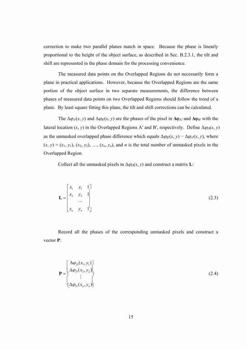
The ∆ϕA′(x, y) and ∆ϕB′(x, y) are the phases of the pixel in ∆ϕA′ and ∆ϕB′ with the
lateral location (x, y) in the Overlapped Regions A′ and B′, respectively. Define ∆ϕD(x, y)
as the unmasked overlapped phase difference which equals ∆ϕB′(x, y) − ∆ϕA′(x, y), where
(x, y) = (x1, y1), (x2, y2), …, (xn, yn), and n is the total number of unmasked pixels in the
Overlapped Region.
Collect all the unmasked pixels in ∆ϕD(x, y) and construct a matrix L:
⎥⎥⎥⎥
⎦
⎤
⎢⎢⎢⎢
⎣
⎡
=
1
11
22
11
nn yx
yxyx
LL (2.3)
Record all the phases of the corresponding unmasked pixels and construct a
vector P:
⎪⎪⎭
⎪⎪⎬
⎫
⎪⎪⎩
⎪⎪⎨
⎧
∆
∆∆
=
),(
),(),(
22
11
nnD
D
D
yx
yxyx
ϕ
ϕϕ
MP (2.4)

16
Fit a least square plane to ∆ϕD, defined by cbyaxyxD ++=∆ ),(ϕ . The
coefficients a, b, and c are determined by:
( ) ( )PLLL TT
cba
1−=
⎪⎭
⎪⎬
⎫
⎪⎩
⎪⎨
⎧ (2.5)
The coefficients a and b relate to the tilt about y and x axes, respectively, of
Measurement B relative to Measurement A. The coefficient c determines the relative
shift of Measurement B relative to Measurement A in z axis.
Once the coefficients, a, b, and c are obtained, the phase ),( yxBϕ∆ of the whole
measurement region in Measurement B is corrected by:
[ ]cbyaxyxyx BcB ++−∆=∆ ),(),( ϕϕ (2.6)
where ),( yxcBϕ∆ is the tilt-corrected phase of ∆ ),( yxBϕ .
In summary, to register two holograms shown in Fig. 2.1, the unmasked
Measurements A and B are first identified. Using the cross-correlation analysis, the
translational shift is calculated and the rectangular Overlapped Regions A′ and B′ are
marked. The phase matrices of two Overlapped Regions are used to find the tilt and shift
between Measurements A and B and complete the data registration.
2.2.3. Rotation
Rotation is the angular movement of the measurement object in the xy plane
between the two measurements. If the rotation occurs with the lateral translation, the
identification and correction of the rotation will be conducted before the lateral
translation which is described in Sec. 2.2.1.

17
2.2.3.1. Rotation identification
The identification of the rotation is implemented using the Fourier transform [32]
of the intensity matrices. Assume the object in the Measurement B is rotated by θ0 and
translated by (xs, ys) relative to the Measurement A, the intensity matrix IB can be
expressed by
)cossin,sincos(),( 0000 ssAB yyxxyxIyxI −+−−+= θθθθ (2.7)
The Fourier transform F of the intensity matrix I is determined by [33]
∑= +−
yx
Nyxjkk eyxI
NF
,
/)(2),(1),( ηξπηξ (2.8)
where k = A or B, and N is the total number of data points.
The relation between FA and FB is determined by
)cossin,sincos(),( 0000)(2 θηθξθηθξηξ ηξπ +−+= +−
Ayxj
B FeF ss (2.9)
From Eq. (2.9), we have
)cossin,sincos(),( 0000 θηθξθηθξηξ +−+= AB MM (2.10)
where MA = |FA| and MB =|FB| are the magnitudes of FA and FB, respectively.
Eq. (2.10) indicates that the matrix MB is rotated by the angle θ0 relative to the
matrix MA in the ζη plane. Convert the Cartesian coordinate (ζ, η) of the matrices MA

18
and MB into the polar coordinate (ρ, θ), where ρ and θ are the magnitude and angle of the
coordinate (ζ, η), respectively. Then the relation between the matrices MA and MB in Eq.
(2.10) is expressed by
),(),( 0θθρθρ += AB MM (2.11)
The rotation θ0 between the two matrices MA and MB is separated from the lateral
translation (xs, ys) using the Eq. (2.11). This rotation can be identified using the cross-
correlation, defined by Eqs. (2.1) and (2.2), of the matrices MA and MB in the ρθ plane.
2.2.3.2. Rotation correction
Once the rotation θ0 of the object between the two measurements is identified
using the method described in Sec. 2.2.3.1, the rotation will be corrected before the
identification of the lateral translation by [33]
⎥⎦
⎤⎢⎣
⎡⎥⎦
⎤⎢⎣
⎡−
=⎥⎦
⎤⎢⎣
⎡yx
yx
r
r
00
00
cossinsincos
θθθθ
(2.12)
where xr and yr are the lateral coordinates after rotation.
Interpolation is required in general after the rotation because the lateral
coordinates (x, y), which are integers in the matrix before the rotation, will not
necessarily be integers after the rotation.
The bilinear interpolation [33] is applied due to the easy implementation and less
computational cost. Assume that the intensity values I11, I12, I21, and I22 at the four
positions (x1, y1), (x1, y2), (x2, y1), and (x2, y2), respectively, are known and the intensity at
the position (x, y) can be estimated by Eq. (2.13), where x1 < x < x2 and y1 < y < y2.

19
))(())((
))(())((
))(())((
))(())((
),(
111212
2212
1212
12
211212
2122
1212
11
yyxxyyxx
Iyyxxyyxx
I
yyxxyyxx
Iyyxxyyxx
IyxI
−−−−
+−−−−
+−−−−
+−−−−
=
(2.13)
2.3. Accuracy evaluation of hologram registration
Two examples using different approaches are applied to evaluate the accuracy of
the proposed hologram registration method. The first approach uses a measurement
object which is small and fits in the FOV. The object can be accurately measured to
create a standard height measurement hs(x, y). The same object is then measured twice
on two sides with an overlapped region in between. The proposed method is applied to
calculate the registered height measurement hm(x, y). The accuracy of the registration
method is quantified by comparing hs(x, y) to hm(x, y). A wheel hub is used as the
Example I.
The other approach uses a measurement object larger than the FOV. The CMM
measurement of the whole measurement object is used as the standard measurement hs(x,
y). It is compared to the registered measurement hm(x, y). An engine combustion deck
surface is used as the Example II.
2.3.1. Accuracy evaluation procedures
Two parameters, the root mean squared (RMS) error erms of the difference
between the hs(x, y) and hm(x, y) and the surface flatness, are used to evaluate the
accuracy of the hologram registration method.
To compare hs(x, y) and hm(x, y), a linear transformation is required to tilt and
shift the hm(x, y) relative to hs(x, y) before calculating erms. Since the measurement
system in this study only delivers the relative height measurement, this linear
transformation is required. Let Fs(x, y) = asx + bsy + cs and Fm(x, j) = amx + bmy + cm be

20
the least square fitted planes of hs(x, y) and hm(x, y), respectively. The linear
transformation of hm(x, y) can be expressed as:
[ ])()()(),(),( smsmsmmTm ccybbxaayxhyxh −+−+−−= . (2.13)
The RMS error erms is:
( )d
yxhyxhe
dd yx
yxyx
Tms
rms
∑ −= =
),(
),(),(
2
11
),(),( (2.14)
where d is the total number of all unmasked pixels.
The surface flatness is also used as an index to evaluate the accuracy. Two
flatness definitions are used in this study. One is 6σ flatness, which is equal to six times
the standard deviation of measured points from the least square fitted plane [34]. This
definition suppresses the spike noise contribution to the flatness. The other is the
maximum peak to valley from the least square fitted plane. This is called the peak-to-
valley flatness.
2.3.2. Example I -- wheel hub
As shown in Fig. 2.2, a wheel hub, which is small to fit the FOV, is used as a
measurement object to evaluate the accuracy of the hologram registration method. Five
bolts were assembled to the wheel hub to transmit power to the wheel. These bolts after
being assembled may alter the original hub surface flatness and need to be inspected.
The laser holographic interferometry is a unique method to measure the surface flatness
of the hub with the assembled bolts. The diameter of the hub, as shown in Fig. 2.2(b), is
about 150 mm.

21
The intensities and phases for each measurement are shown in Fig. 2.3. The solid
black regions in Figs. 2.3(a) and 2.3(b) are masked and excluded for height measurement.
The intensity matrices IA and IB have the dimension of 649 x 964 and 615 x 964 pixels,
respectively.
The cross-correlation matrix C of IA and IB is represented in Fig. 2.4. The
dimension of C is 1297 x 1927 pixels. The location of the correlation peak is identified
at (301, 964). This indicates that the measurement matrix A should translate 301 − 649 =
−348 pixels in +x direction and 964 − 964 = 0 pixels in the +y direction to make the
strongest match with the measurement matrix B. With this translational movement, the
Overlapped Regions A′ and B′ can be chosen from the measurements A and B,
respectively.
The hologram phase ∆ϕA′ and ∆ϕB′ of the Overlapped Regions A′ and B′,
respectively, are shown in Fig. 2.3(b) in dashed rectangles. The reference point is
marked with a plus sign. The dimension NA΄ x MA΄ of the Overlapped Regions is 300 x
964 pixels. The relative tilt and shift parameters [a, b, c], defined in Eq. (2.5), are
[−1.0×10⁻⁴ rad/pixel, 1.2×10⁻⁵ rad/pixel, 1.23×10⁻² rad]. Correct the relative tilt using
Eq. (2.6) and register two holograms. The phase and intensity of the registered hologram
are shown in Fig. 2.5. A clear separation line between two measurements can be
observed in the registered intensity, as shown in Fig. 2.5(b). This is because the intensity
of the Measurements A and B are connected without any correction. This does not affect
the height measurement, which is calculated from the registered phase, as shown in Fig.
2.5(a).
There is a dent on the hub surface, which is marked in Fig. 2.2(b) and shown in
close-up view in Fig. 2.2(c). Because this dent is more than 9 pixels in the image, this
cannot be eliminated by 9 point median filtering. The 6σ surface flatness definition is
applied to suppress the effect of this dent on the surface flatness measurement results.
Interpolation is applied to achieve sub-pixel resolution for the hologram
registration. First, the lateral cross-correlation process, defined in Eq. (2.2), is
interpolated. For example, one point linear interpolation is utilized in the 300 x 964

22
pixels overlapped region. The lateral translation is the same after processing. For higher
sub-pixel resolution, two or more points can be linear interpolated.
The registered height measurement hm(x, y) is shown in Fig. 2.6(a). The standard
measurement hs(x, y), as shown in Fig. 2.6(b), is obtained in a single holographic
interferometry measurement of the wheel hub, which is small to fit in the FOV. The 6σ
flatness of hs(x, y) and hm(x, y) are 25.3 and 25.2 µm, respectively. The gage repeatability
(1σ ) of the system is evaluated as 0.3 µm. Compared to this value, the 0.1 µm or 0.4%
flatness difference is not significant. It indicates that the hologram registration does not
significantly contribute to the measurement error.
The difference between hs(x, y) and hm(x, y) is presented in Fig. 2.7. The RMS
value erms is 0.4 µm. This further proves the accuracy of the proposed hologram
registration method.
The effect of the area of the overlapped region was also evaluated. As shown in
Fig. 2.8, hologram registration with 10, 25, and 40% of the overlapped vs. total
measurement area were conducted with the corresponding erms of 0.9, 0.5 and 0.4 µm,
respectively. As the area of the overlapped region increases, the error introduced by the
registration method decreases. The increase of overlapped region from 10 to 25%
reduces the erms by 0.4 µm. The same 15% increase of overlapped region from 25 to 40%
only reduces the erms by 0.1 µm. Also, when the area of the overlapped region is larger
than 40%, the error erms is approaching the 0.3 µm system error. It is expected that
increasing the overlapped region beyond 40% will not reduce erms significantly.
2.3.3. Example II -- engine head combustion deck surface
As shown in Fig. 2.9, an engine head combustion deck surface has a large, 420 x
180 mm, measurement area. Two measurements, marked as Measurements A and B in
Fig. 2.9, were conducted. The translation of the measurement object was achieved by
moving it with the side datum surface of the measurement object in contact with a
straight reference bar in the machine. The intensity matrices IA and IB have dimensions
of 948 x 584 and 889 x 599 pixels, respectively. Following the cross-correlation

23
procedure, the overlapped region with the size of 598 x 458 pixels is identified. The
relative tilt and phase shift parameters [a, b, c], defined in Eq. (2.5), are [4.5×10⁻⁴
rad/pixel, 3.1×10⁻³ rad/pixel, −0.5 rad]. The tilt and phase shift are corrected using Eq.
(2.6) and the two measurements are registered as a 1378 x 599 matrix.
The 3D profile of the registered surface is shown in Fig. 2.10(a). In comparison,
the same surface was measured by a Zeiss Model UPMC 850 CMM with a scanning
probe. The CMM measurement, which covers only a small portion of the surface, is
shown in Fig. 2.10(b).
The peak-to-valley flatness definition is applied for evaluation because the surface
area measured by CMM and laser holographic interferometry is significantly different.
Under such condition, the standard deviation does not provide a comparable
representation of measurement results. The peak-to-valley flatness of the CMM and the
registered laser holographic measurement are 149.7 and 153.5 µm, respectively. This
close comparison, 2.5% discrepancy, further verifies that the developed hologram
registration method is feasible for the precision measurement of large components.
2.4. Concluding remarks
This research developed a hologram registration method for the laser holographic
interferometry to measure the 3D profile of objects larger than the FOV. Two examples
were used to validate the registration method using two different approaches. The first
example, a wheel hub, was smaller than the FOV and enabled the use of holographic
interferometry to create the standard measurement for the accuracy evaluation of
hologram registration. The second example, an engine head combustion deck surface,
was larger than the FOV and a CMM was used to create the standard measurement. The
erms was 0.4 µm for the wheel hub (Example I) and peak-to-valley flatness difference was
about 4 µm for the engine head combustion deck surface (Example II). The feasibility of
the proposed hologram registration method was demonstrated.
The unique feature of the proposed registration method is the elimination of using
target for data registration. This could simplify the measurement procedure and reduce

24
the time. Several research investigations can follow this study. The robustness of the
proposed registration method with more complex surface geometric shapes than
examples of the wheel hub and engine combustion deck surfaces is a good future research
topic. The limit of the tilt and shift and optimal percentage of the area of the overlapped
region can also be investigated as a series of follow-up research for practical application
of the proposed hologram registration method. Only two measurements are used for the
hologram registration examples in this study. A more comprehensive program to register
multiple holograms can be developed and the error propagation analysis can be
conducted to further advance the capability of hologram registration for precision
measurements.

25
Field of View
xy
pW
pW
Measurement AOverlapped Region A'
pMA
pMA
'
pNA
pNA'
Field of View
xy
pW
Measurement BOverlapped Region B'
pMB
pMB
'
pNB
pNB'
(a) (b)
Fig. 2.1. Measurement regions and variables used for hologram registration: (a) Measurement A and (b) Measurement B. In this research, W = 1024, p = 0.293 mm, and
pW = 300 mm.
Measurement object

26
(a) (b)
(c)
Fig. 2.2. Wheel hub: (a) isometric view, (b) top view, and (c) close-up view of the dent marked in solid rectangle in (b).
Ø150 mm
Measurement A Measurement B
4 mm
Overlapped Region

27
(a)
(b)
Fig. 2.3. Measured holograms of the wheel hub: (a) intensity and (b) phase of Measurements A and B.
Reference point Reference point
649 pixels 615 pixels
964
pixe
ls
Phase ∆ϕA΄ of overlapped region Phase ∆ϕB΄ of overlapped region
Intensity IA
Intensity Intensity
Intensity IB
300 pixels
964
pixe
ls
300 pixels

28
Fig. 2.4. Correlation matrix C of Measurements A and B of the wheel hub.
Correlation peak

29
(a)
(b)
Fig. 2.5. Registered hologram of the wheel hub: (a) phase and (b) intensity.
964
pixe
ls
Intensity

30
(a) (b)
Fig. 2.6. 3D profile measurement of the wheel hub: (a) registered measurement hm(x, y) and (b) standard measurement hs(x, y).
Fig. 2.7. Difference between hs(x, y) and hm(x, y) of the wheel hub.
6σ Flatness: 25.3 µm 6σ Flatness: 25.2 µm
µ µ
µ

31
00.10.20.30.40.50.60.70.80.9
1
0% 5% 10% 15% 20% 25% 30% 35% 40% 45%
Percentage of the area of the overlapped region
Erro
r erm
s ( µ
m)
Fig. 2.8. Effect of the area of the overlapped region on the error erms.
Fig. 2.9. Overview of a V6 engine head combustion deck surface.
Measurement A Measurement B
420 mm
180
mm
Overlapped Region

32
(a)
(b)
Fig. 2.10. 3D profile of the engine head combustion deck surface: (a) registered measurement and (b) CMM measurement.
Peak-to-valley flatness: 149.7 µm
Peak-to-valley flatness: 153.5 µm

33
Chapter 3
Phase Unwrapping for Large Depth-of-Field 3D Laser Holographic Interferometry Measurement of Laterally Discontinuous Surfaces
3.1. Introduction
Phase unwrapping is a mathematical procedure to eliminate the ambiguity in the
phase map for imaging applications, including the synthetic aperture radar interferometry,
laser holographic interferometry, magnetic resonance imaging, and others [35]. In this
research, phase unwrapping is studied to increase the depth-of-field for the 3D laser
holographic interferometry measurement of laterally discontinuous surfaces. The phases
calculated by the laser holographic interferometry range from –π to π, the principal value
range of reverse trigonometric functions. The limited range of phase creates ambiguity,
called phase wrap. Fig. 3.1(a) shows an example of a parabolic-shaped surface with
phases ranging from 0 to 18 radians. The measurement of this surface with phase wraps
is shown in Fig. 3.1(b). Sudden changes of phase are observed at pixels with the phase
value near –π or π. Phase unwrapping restores the true phase map (Fig. 3.1(a)) from the
measured phase map (Fig. 3.1(b)). If the spatial sampling rate in the phase map is at least
twice of the highest frequency of the change of phase, so called Shannon sampling
theorem [36], a phase wrap is assumed when the phase difference between two adjacent
pixels exceeds the threshold π. The wrapped phase is compensated by the integral
multiples of 2π to be unwrapped.
The technical advancements in phase unwrapping have been aimed to achieve the
high noise robustness and low computational cost. Both temporal- and spatial-based
approaches for phase unwrapping have been developed. Temporal-based phase
unwrapping, developed by Huntley and Saldner [36,37], unwraps the change of phase
over time for each pixel independently. The error is restricted to individual pixels and

34
does not propagate between pixels. Special optical configurations [38] are required to
relate the unwrapped phase to the height of surface and it makes the temporal-based
approach not suitable for the laser holographic interferometry measurement, the targeted
application in this research.
Spatial-based phase unwrapping processes the phase in the 2D spatial domain
using either path-dependent or path-independent methods. The path dependent method
unwraps the phase along a specially designed path by converting the 2D array into a
folded 1D data set. This method needs complex path design strategy in the presence of
noise [39] and is not feasible for the measurement of the laterally discontinuous surface,
which contains regions disconnected with each other. Information between disconnected
regions is unavailable along the designed path. The automatic transmission valve body,
as shown in Fig. 3.2(a), has the laterally discontinuous surface. Figure 3.2(b) shows the
top view of the measurement surface of a valve body. It contains grooves which carry
pressurized fluid to control the position of valves for gear shifting. The surface with high
aspect ratio regions disconnected with each other makes the phase unwrapping difficult.
The spatial-based path-independent methods, including model- [40,41], Bayesian-
[42], least-squares- [43], and integration-based [44-52], do not require a specially
designed path for the phase unwrapping. However, none of these spatial-based path-
independent methods can be directly applied to unwrap the phase of laterally
discontinuous surfaces because of narrow, curved regions and the discontinuity among
regions. The region-referenced method [52], which is an integration-based and path-
independent method, uses the phase data in regions surrounding a pixel to detect the
phase wrap. This method has good noise robustness, can automatically adjust the
direction to adapt for narrow and curved regions, and is selected to be further developed
in this study.
The region-referenced phase unwrapping, segmentation and patching, and its
problems for narrow segmented regions and boundary pixels are explained in Sec. 3.2. In
Sec. 3.3, the solutions of phase wrap identification on boundary pixels, masking and
recovery, dynamic segmentation, and phase adjustment are developed. An example is

35
presented in Sec. 3.4 to validate the proposed method and study the computational
efficiency and convergence.
3.2. Region-referenced phase unwrapping
The region-referenced method is applied as the base for the developed phase
unwrapping method. The region-referenced method uses an iterative algorithm to
unwrap the phase. This method searches the pixels with phase wraps and compensates
the phase by adding or subtracting 2π depending on the sign of phase wrap. The surface
is assumed continuous in the height direction with no phase jump over π between two
adjacent pixels. The searching and compensation processes are repeated until no phase
wrap is detected.
3.2.1. Principle
A simple method to determine the phase wrap is to use the four adjacent pixels of
a pixel, marked as (i, j) in Fig. 3.3(a), to determine the phase wrap [39,54]. If at least one
of the four adjacent pixels has the phase difference larger than π, this pixel is recognized
to have phase wrap and needs to be compensated by adding or subtracting 2π for phase
unwrapping. The problem of this phase unwrapping method is the sensitivity to noise,
which can cause the divergence of the iteration. A more complicated region-referenced
criterion is developed by Huang and He [52] to overcome this problem. Each adjacent
pixel in Fig. 3.3(a) is replaced by a region to determine the phase wrap. For example, the
adjacent pixel (i−1, j) in Fig. 3.3(a) is replaced by 15 pixels, as shown by the shaded area
in Fig. 3.3(b), to determine the phase wrap. If over half of the pixels in the shaded region
have the phase difference larger than π with the pixel (i, j), a phase wrap is identified at
pixel (i, j). The criterion of over half of pixels, which is 8 in the case in Fig. 3.3(b), is
empirically optimal [52]. Rotating the shaded region around the pixel (i, j) by 90, 180,
and 270º, the other three reference regions corresponding to the other three adjacent
pixels in Fig. 3.3(a) can be obtained. The phase wrap at pixel (i, j) is identified if any of
the four reference regions have the phase wrap. Other reference regions of different

36
shapes are also developed [52]. This method can significantly improve the noise
robustness. However, pixels on the boundary, so called boundary pixels, have limited
number of pixels in the reference region to detect the phase wrap. This makes boundary
pixels more sensitive to noise. The laterally discontinuous surface, like the automatic
transmission valve body in Fig. 3.2, has many boundary pixels due to the discontinuity
between regions, and may introduce the divergence problem in phase unwrapping.
Figure 3.4 shows the measured phase map of the automatic transmission valve
body. The solid black background is the region not for measurement. All the phase
values are within the range from –π to π, the principal value range of reverse
trigonometric functions. Phase wraps are observed in the phase map. The close-up view
of the region S1 is shown in Fig. 3.5(a). The boundary pixels, marked by arrows, are a
source of instability and make the region-referenced phase unwrapping easy to diverge.
The idea proposed in this research is to first conduct the phase unwrapping without
considering these boundary pixels, i.e., boundary pixels with phase wrap are masked.
After phase unwrapping, these masked pixels are recovered by median filtering. This
concept will be elaborated in Sec. 3.3.1.
3.2.2. Segmentation and patching
Segmentation, which divides the phase map into many small overlapped segments,
has been developed to improve the computational efficiency for phase unwrapping
[50,52]. Each segment is first unwrapped independently. Then, the data of two adjacent
segments is connected using the overlapped region between these two segments. The
static segmentation is defined as the segmentation method with fixed size of segments
and overlapped regions during unwrapping.
Patching is the process to combine the data of individual segments after phase
unwrapping into an integral phase map. Two adjacent segments with an overlapped
region are compared with each other and the phases of one segment are shifted by the
multiple of 2π to make the overlapped regions of the two segments match. After shifting,
these two adjacent segments are concatenated. This procedure is applied to all the
adjacent segments until an integral phase map including all the individual segments is

37
reached. The path which the patching process follows is determined iteratively by
systematically selecting one of the four adjacent segments as the next segment to be
patched.
An example of static segmentation with patching is shown in Fig. 3.6(a), which
illustrates the close-up view of region S2 of the valve body in Fig. 3.4. The size of each
segment is (W + Wo) x (W + Wo) with the width of the overlapped region equal to Wo.
The unwrapped phase in segments C1D1E1F1 and C2D2E2F2 will be patched by shifting
the phases of the segment C1D1E1F1 relative to the segment C2D2E2F2 to make the
overlapped region C2D1E1F2 matches in both C1D1E1F1 and C2D2E2F2.
The problem of the static segmentation for laterally discontinuous surfaces is the
thin boundary regions. An example of the boundary region is shown in Fig. 3.6(b),
which is the close-up view of the region S4 in Fig. 3.6(a). A boundary region with only 1
to 2 pixels in width after static segmentation and patching is observed on the top of the
segment. The phase wrap which exists in this boundary region cannot be detected or
removed using the phase unwrapping method. The dynamic segmentation and the phase
adjustment, to be discussed in Secs. 3.3.3 and 3.3.4, respectively, are developed to
overcome this problem.
3.3. Masking, dynamic segmentation and phase adjustment
The masking and recovery, dynamic segmentation, and phase adjustment are
developed to improve the robustness and the computational efficiency for phase
unwrapping of laterally discontinuous surfaces. To avoid the divergence problem,
boundary pixels with phase wrap are masked during phase unwrapping. These pixels are
recovered after phase unwrapping. Dynamic segmentation adaptively determines the size
of segments to reduce the number of thin boundary regions in segmentation. The phase
adjustment corrects the errors after dynamic segmentation to complete phase unwrapping.

38
3.3.1. Phase wrap identification on boundary pixels
To determine if a boundary pixel has phase wrap, a criterion is developed. Each
boundary pixel has four reference regions. In each reference region, some pixels are not
on the object surface, and do not have valid phase information. Those pixels with valid
phase information are denoted as valid pixels. If more than half of the valid pixels in any
of the four reference regions of a boundary pixel have the phase difference larger than π,
this boundary pixel is designated to have the phase wrap and will be masked in the phase
unwrapping.
3.3.2. Masking and recovery
Masking is applied on the boundary pixels with phase wrap to avoid the
divergence. The masked boundary pixels with phase wrap are not processed for the
phase unwrapping. However, the masked boundary pixel is still a valid pixel and its
phase information is used in reference regions of other pixels for phase unwrapping
analysis.
After phase unwrapping, to recover the value at a masked boundary pixel, the
median filtering [55] is applied. Median filtering first sorts the phase values of pixels in a
matrix (usually 3x3, 5x5, 7x7, or 9x9 in dimension) centered at the pixel and then
chooses the median as the new phase value. If any of the pixels in the matrix have been
masked, values of these pixels are not included in the sorting sequence. Median filtering
has the advantage of suppressing the spike noise.
An example of the masking and recovery process is illustrated in Fig. 3.5. Figure
3.5(a) shows the close-up view of the region S1 in Fig. 3.4. Boundary pixels with phase
wrap are marked by arrows. These pixels are masked for the phase unwrapping. Fig.
3.5(b) shows the result after phase unwrapping and before the recovery. Seven masked
boundary pixels still have the phase wrap before the recovery. The recovery process
assigns the phase values to the masked pixels using a 7x7 median filter. The result after
applying the median filtering is shown in Fig. 3.5(c). The phase unwrapping is
completed without divergence problem and the phase values of the masked boundary
pixels have been recovered.

39
3.3.3. Dynamic segmentation
The static segmentation, as discussed in Sec. 3.2.2, has fixed size of segments and
fixed width of overlapped regions. Dynamic segmentation is developed in this study to
overcome the problem of thin boundary regions of laterally discontinuous surfaces.
To identify the thin boundary region, the width of boundary regions needs to be
quantified. A parameter, called the boundary width pm, of each boundary region is
defined as the maximum number of pixels inside the boundary region in the direction
perpendicular to the side of the segment. An example is shown in Fig. 3.7(a). Two
unmasked boundary regions, marked by the hatched lines, have pm equal to pm1 and pm2,
respectively. The smaller of the two, pm1, is denoted as the minimum side width pmin,
which is defined as the minimum of the boundary widths of all the boundary regions on a
side of the segment.
An exception in the determination of pm occurs when a narrow region exists along
the two adjacent sides. As shown in Fig. 3.7(b), the pixels, which are on the top side of
the segment and are close (less than a predetermined threshold T) to the left side of the
segment, are not considered in the calculation of the pm3. In Fig. 3.7(b), the smaller of
pm3 and pm4 is used to determine the pmin to represent the minimum boundary width of the
top side of the rectangular segment.
Dynamic segmentation starts with the static segmentation. If one side of a
segment has pmin smaller than T after the static segmentation, dynamic segmentation is
triggered. The side of the segment after the static segmentation will be moved toward
outside of the segment by m1 = (T – pmin) pixels to increase the width of the thin boundary
region. The counting of pmin is applied again to identify if any thin boundary region still
exists on the new segment. If it does, the side of the segment is moved in the opposite
direction by m2 = m1 + T/2 pixels. This dynamic segmentation is repeated to all four
sides of the rectangular segment and has demonstrated the ability to eliminate most, but
not all, of the thin boundary regions in practical applications.
Figure 3.8 shows an example of the dynamic segmentation of the region S3 in Fig.
3.4. The size of segments and the width of overlapped regions are W = 50 and Wo = 20
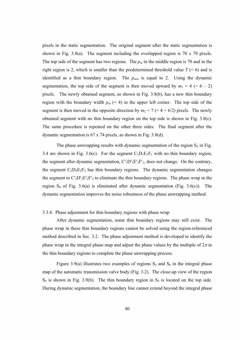
40
pixels in the static segmentation. The original segment after the static segmentation is
shown in Fig. 3.8(a). The segment including the overlapped region is 70 x 70 pixels.
The top side of the segment has two regions. The pm in the middle region is 70 and in the
right region is 2, which is smaller than the predetermined threshold value T (= 6) and is
identified as a thin boundary region. The pmin is equal to 2. Using the dynamic
segmentation, the top side of the segment is then moved upward by m1 = 4 (= 6 – 2)
pixels. The newly obtained segment, as shown in Fig. 3.8(b), has a new thin boundary
region with the boundary width pm (= 4) in the upper left corner. The top side of the
segment is then moved in the opposite direction by m2 = 7 (= 4 + 6/2) pixels. The newly
obtained segment with no thin boundary region on the top side is shown in Fig. 3.8(c).
The same procedure is repeated on the other three sides. The final segment after the
dynamic segmentation is 67 x 74 pixels, as shown in Fig. 3.8(d).
The phase unwrapping results with dynamic segmentation of the region S2 in Fig.
3.4 are shown in Fig. 3.6(c). For the segment C1D1E1F1 with no thin boundary region,
the segment after dynamic segmentation, C′1D′1E′1F′1, does not change. On the contrary,
the segment C2D2E2F2 has thin boundary regions. The dynamic segmentation changes
the segment to C′2D′2E′2F′2 to eliminate the thin boundary regions. The phase wrap in the
region S4 of Fig. 3.6(a) is eliminated after dynamic segmentation (Fig. 3.6(c)). The
dynamic segmentation improves the noise robustness of the phase unwrapping method.
3.3.4. Phase adjustment for thin boundary regions with phase wrap
After dynamic segmentation, some thin boundary regions may still exist. The
phase wrap in these thin boundary regions cannot be solved using the region-referenced
method described in Sec. 3.2. The phase adjustment method is developed to identify the
phase wrap in the integral phase map and adjust the phase values by the multiple of 2π in
the thin boundary regions to complete the phase unwrapping process.
Figure 3.9(a) illustrates two examples of regions S5 and S6 in the integral phase
map of the automatic transmission valve body (Fig. 3.2). The close-up view of the region
S5 is shown in Fig. 3.9(b). The thin boundary region in S5 is located on the top side.
During dynamic segmentation, the boundary line cannot extend beyond the integral phase

41
map and the thin boundary region exists. The close-up view of S6 is shown in Fig. 3.9(c).
The thin boundary region with phase wrap still exists after moving the boundary line
twice in dynamic segmentation.
The phase values of pixels in thin boundary regions can be estimated or
extrapolated using a polynomial function fitted by the data of the integral phase map. If
the difference between the estimated phase values and the existing phases of pixels in
thin boundary regions is larger than 2π, the multiple of 2π is subtracted to the existing
phases to make the difference smaller than 2π. The polynomial function can be of the
first, second, third, or higher order. The first order polynomial function representation of
the integral phase map is:
1 0,1 1,1 2,1( , )i j a a i a jϕ = + + (3.1)
where
ϕ1(i, j) is the estimated phase value of the pixel (i, j) in the integral phase map,
i and j are the row and column coordinates, respectively, of the integral phase map,
and
a0,1, a1,1, and a2,1 are the coefficients of the first order polynomial function,
determined using the least square estimation [56]:
⎪⎭
⎪⎬
⎫
⎪⎩
⎪⎨
⎧
∑∑∑
⎥⎥⎥
⎦
⎤
⎢⎢⎢
⎣
⎡
∑∑∑∑∑∑∑∑∑
=⎪⎭
⎪⎬
⎫
⎪⎩
⎪⎨
⎧ −
1
1
11
2
2
1,2
1,1
1,0 1
ϕϕϕ
ji
jijjijiiji
aaa
(3.2)
The second order polynomial function of ϕ(i, j) is:

42
2 22 0,2 1,2 2,2 3,2 4,2 5,2( , )i j a a i a j a i a ij a jϕ = + + + + + (3.3)
where a0,2, a1,2, a2,2, a3,2, a4,2, and a5,2 are estimated by [56]:
⎪⎪⎪⎪
⎭
⎪⎪⎪⎪
⎬
⎫
⎪⎪⎪⎪
⎩
⎪⎪⎪⎪
⎨
⎧
∑∑∑∑∑∑
⎥⎥⎥⎥⎥⎥⎥⎥
⎦
⎤
⎢⎢⎢⎢⎢⎢⎢⎢
⎣
⎡
∑∑∑∑∑∑∑∑∑∑∑∑
∑∑∑∑∑∑∑∑∑∑∑∑∑∑∑∑∑∑∑∑∑∑∑∑
=
⎪⎪⎪⎪
⎭
⎪⎪⎪⎪
⎬
⎫
⎪⎪⎪⎪
⎩
⎪⎪⎪⎪
⎨
⎧−
22
2
22
2
2
21
4322322
322322
2234232
3222
2232
22
2,5
2,4
2,3
2,2
2,1
2,0 1
ϕϕϕϕϕϕ
jijiji
jijjijijjijjijiijjiij
jijiijiiijijjijijj
ijjiiijiijijiji
aaaaaa
(3.4)
The third order polynomial function is defined by:
2 2 3 2 2 33 0,3 1,3 2,3 3,3 4,3 5,3 6,3 7,3 8,3 9,3( , )i j a a i a j a i a ij a j a i a i j a ij a jϕ = + + + + + + + + + (3.5)
where a0,3, a1,3, a2,3, a3,3, a4,3, a5,3, a6,3, a7,3, a8,3, and a9,3 are the coefficients to be
estimated by the same least square estimation principle [56].
To determine which order polynomial is adequate for the phase adjustment, the
root mean square erms, defined by Eq. (3.6), of the estimation error is applied.
( )N
jijie ji
k
rms
∑ −= ,
2),(),( ϕϕ (3.6)
where k is the order of the polynomial function and N is the total number of data points in
the integral phase map.

43
If the erms is small than a predefined threshold (for example, 0.2 rad which is
experimentally verified to be sufficient in this study), the polynomial function is
considered adequate for the phase adjustment. Otherwise, higher order polynomial
function will be fitted using the least square method [56] until the erms is smaller than the
threshold.
3.4. Example
The measurement of the surface on an automatic transmission valve body, as
shown in Fig. 3.2, is used as an example of the laterally discontinuous surface to
demonstrate the developed phase unwrapping method. The measurement area, as shown
in Fig. 3.2(b), was 265 x 250 mm. The measurement result was represented in a matrix
with the dimension of 892 x 842 pixels. The height measurement range was set as 0.3
mm. The lower right corner of the valve body was raised by a wedge to increase the
height range of the valve body surface beyond 0.3 mm and generate the phase wrap.
3.4.1. Phase unwrapping results
The measured phase map is shown in Fig. 3.4. To unwrap the measured phase
map in Fig. 3.4, the region-referenced phase unwrapping method described in Sec. 3.2 is
applied. The 15 pixels reference region, as shown in Fig. 3.3(b), is utilized to identify the
phase wrap. For each pixel, if more than 8 pixels in any of the four reference regions
have the phase difference larger than 2π, that pixel is marked to have phase wrap. The
masking and the 7x7 median filter for recovery, as discussed in Sec. 3.3.2, are applied on
those boundary pixels with phase wrap to avoid the divergence problem on boundary
pixels.
The dynamic segmentation with W = 50 pixels, Wo = 15 pixels, and T = 6 pixels,
is applied to generate 18x17 (=306) segments. This segmentation generates 71 thin
boundary regions. The dynamic segmentation is applied to move all four sides (top,
bottom, right, and left) of the segments to reduce the number of thin boundary regions.
In this example, 53 segments have at least one of the four sides moved once and 3

44
segments have at least one of the four sides moved twice. After the dynamic
segmentation, only 5 thin boundary regions exist. These remaining thin boundary regions
are marked by three arrows and two boxes (S5 and S6) in Fig. 3.9(a). Figures 3.9(b) and
3.9(c) illustrate the close-up view of the thin boundary regions in S5 and S6.
The dynamic segmentation was necessary to achieve a converged solution to
phase unwrapping in this example. If only the static segmentation was used, the integral
phase map was incorrect and the phase adjustment could not correct the errors in the
integral phase map.
To recover the phase values in the five thin boundary regions shown in Fig. 3.9(a),
the first and second order polynomial functions were applied to fit the integral phase map.
Results of the fitted polynomial functions are ϕ1(i, j) = –1.521 + 0.006i + 0.013j with a0,1
= –1.521, a1,1 = 0.006, and a2,1 = 0.013, and ϕ2(i, j) = –0.497 + 0.003i + 0.010j + 4×10⁻⁶i2
+ 1×10⁻⁷ij + 4×10⁻⁶j2 with a0,2 = –0.497, a1,2 = 0.003, a2,2 = 0.010, a3,2 = 4×10⁻⁶, a4,2 =
1×10⁻⁷, and a5,2 = 4×10⁻⁶.
The root mean square erms is calculated to determine which order of the
polynomial function is adequate for the phase adjustment. The erms for the first and
second order polynomials are 0.33 rad and 0.16 rad, respectively, with the total number
of data points N = 191131. Because the second order polynomial has the erms smaller
than the predefined threshold 0.2 rad, this polynomial is used for the phase adjustment.
The difference is calculated between the existing phase values and the estimated
values of ϕ2(i, j) in the thin boundary regions. The multiple of 2π is added to or
subtracted from those pixels in the thin boundary regions to make the difference smaller
than 2π. For example, in S5 and S6, 2π was subtracted from both regions to bring the
phase values from the level of 15 rad to 9 rad and from the 9 rad to 3 rad, respectively.
Figure 3.9(d) shows the integral phase map after the phase adjustment. The close-up
views of the two regions S΄5 and S΄6 in Fig. 3.9(d) are shown in Figs. 3.9(e) and 3.9(f),
respectively. The errors have been removed and the whole phase unwrapping process is
complete.

45
3.4.2. Effect of W and Wo on computational efficiency
Two sets of the numerical experiments to study the effect of W and Wo on
computational efficiency are conducted and results are summarized in Table 3.1. The Wo
is fixed at 25 pixels in the first set of test. The reduction of W from 150 to 30 pixels
improves the computational time from 38 to 15 minutes using a common personal
computer with the MATLAB software. A smaller size segment requires less
computational time for phase unwrapping. However, reducing W increases the number of
segments and will eventually increase the computational time. As shown in Table 3.1,
when W is reduced to 29 pixels, the computation time is increased to 16 min. When W is
smaller than 29 pixels, the phase unwrapping method diverges.
The second set of the numerical experiment is conducted by fixing W and
reducing Wo. With a fixed W at 40 pixels, as shown in Table 3.1, the reduction of Wo
from 25 to 10 pixels further reduces the computational time to 6 min while the number of
segments remains the same at 506. As Wo reduces, the size of segments after dynamic
segmentation becomes smaller and makes the phase unwrapping of each segment faster.
The total computational time is reduced. When Wo is smaller than 10 pixels (W = 40
pixels), the divergence problem occurs.
3.4.3. Convergence
The convergence of the phase unwrapping method is also investigated. As shown
in Table 3.2, for W at 50, 40, and 29, the minimum Wo without the divergence problem
are 10, 10, and 24, respectively, for the automatic transmission valve body example.
When W reduces from 50 to 40 pixels, the minimum Wo is the same (10 pixels) to make
the phase unwrapping method converge. When W reduces from 40 to 29 pixels, the
minimum Wo increases to 24 pixels. This is likely due to the increase in the number of
boundary pixels in smaller segments makes the region-referenced phase unwrapping
more prone to divergence.
This example demonstrates the importance of selecting W and Wo to improve
computational efficiency without compromising the stability in phase unwrapping. The
selection of W and Wo will change for different applications. The basic principle learned

46
in this example is to use an optimal W which balances the number of segments and
computational time in each segment. Small Wo without triggering the instability is
desired.
3.5. Concluding remarks
A new phase unwrapping method was developed to mathematically increase the
height measurement range of the laser holographic interferometry while maintaining the
same level of accuracy and resolution. This method had successfully solved the phase
unwrapping problem of the laterally discontinuous surfaces using an example of the
automatic transmission valve body. Three new approaches, including the masking and
recovery, dynamic segmentation, and phase adjustment for pixels in thin boundary
regions, had demonstrated to be effective to avoid the divergence problem of boundary
pixels. A guideline was developed to select the size of segment for improving the
computational efficiency without convergence problem.
This phase unwrapping method, together with the hologram registration method
developed by Huang et al. [53], can successfully increase the measurement volume for
laser holographic interferometry measurements. The phase unwrapping method increases
the height and the hologram registration method expands the field of view.
Two research investigations can be further developed to advance the laser
holographic interferometry measurement system. For measuring objects with height
discontinuity, the 3D CAD model or predetermined (a priori) value on the discontinuity
point can be used in phase unwrapping. The adaptive filtering of the phase map [58] can
also be applied to improve the noise robustness.

47
Table 3.1. Computational time for phase unwrapping of the automatic transmission valve body example (892 x 842 pixels).
Size of segments, W (pixels)
Width of overlapped regions, Wo (pixels)
Number of segments
Computational time (min)
150 25 36 38
100 25 81 25
50 25 306 18
40 25 506 15
30 25 870 15
29 25 930 16
40 20 506 12
40 15 506 9
40 10 506 6
Table 3.2. Minimum Wo for phase unwrapping without divergence in the automatic transmission valve body example.
W (pixels) Minimum Wo (pixels) without divergence
50 10
40 10
29 24

48
(a)
(b)
Fig. 3.1. Artificially created phase map: (a) 3D true phase map without phase wrap and (b) 3D wrapped phase map.

49
(a)
(b)
Fig. 3.2. The automatic transmission valve body: (a) isometric view and (b) top view.
350
mm
265
mm
250 mm

50
(i, j)(i-1, j)
(i, j+1)
(i+1, j)
(i, j-1)
(i, j)
(a) (b)
Fig. 3.3. Detection of phase wrap at pixel (i, j): (a) surrounding four pixels and (b) reference region surrounding the pixel.

51
Fig. 3.4. Measured phase map with phase wrap for the automatic transmission valve body.
842 pixels
892
pixe
ls
S1
S2
S3

52
(a)
(b)
(c)
Fig. 3.5. Close-up view of the region S1 in Fig. 3.4 as an example of the boundary pixels with decreased noise robustness in the detection of phase wrap: (a) before phase unwrapping, (b) after phase unwrapping and before recovery, and (c) after phase
unwrapping and recovery.
: Boundary pixels with phase wrap

53
(a) (b)
(c)
Fig. 3.6. Segmentation: (a) static segmentation of the region S2 in Fig. 3.4, (b) close-up view of the region S4 in Fig. 3.6(a), and (c) dynamic segmentation of the region S2 in Fig.
3.4.
W Wo
C′1 D′1
E′1F′1
C′2 D′2
E′2 F′2
C1 D1
E1 F1
C2 D2
E2 F2
S4

54
(a)
(b)
Fig. 3.7. Definition of the boundary width pm: (a) two boundary regions and (b) the condition with pixels on the top side close to the left side of the segment.
p m1
p m3
p m2
p m4

55
(a) (b)
(c) (d)
Fig. 3.8. Example of the dynamic segmentation of region S3 in Fig. 3.4 (W = 50, Wo = 20, and T = 6 pixels).
70 pixels
70 pixels
67 p
ixel
s
67 p
ixel
s
74 pixels
70 p
ixel
s
70 pixels 74
pix
els

56
(a) (c)
(d) (f)
Fig. 3.9. Phase unwrapping of the automatic transmission valve body: (a) unwrapped phase map without adjustment, (b) close-up view of the region S5 in (a), (c) close-up
view of the region S6 in (a), (d) unwrapped phase map after adjustment, (e) close-up view of the region S΄5 in (d) after adjustment, and (f) close-up view of the region S΄6 in (d)
after adjustment.
S5
S6
(e) S΄6
S΄5
(b)
Thin Boundary Region with phase wrap
Thin Boundary Region with phase wrap
S5
S6
S΄5
S΄6
: thin boundary regions
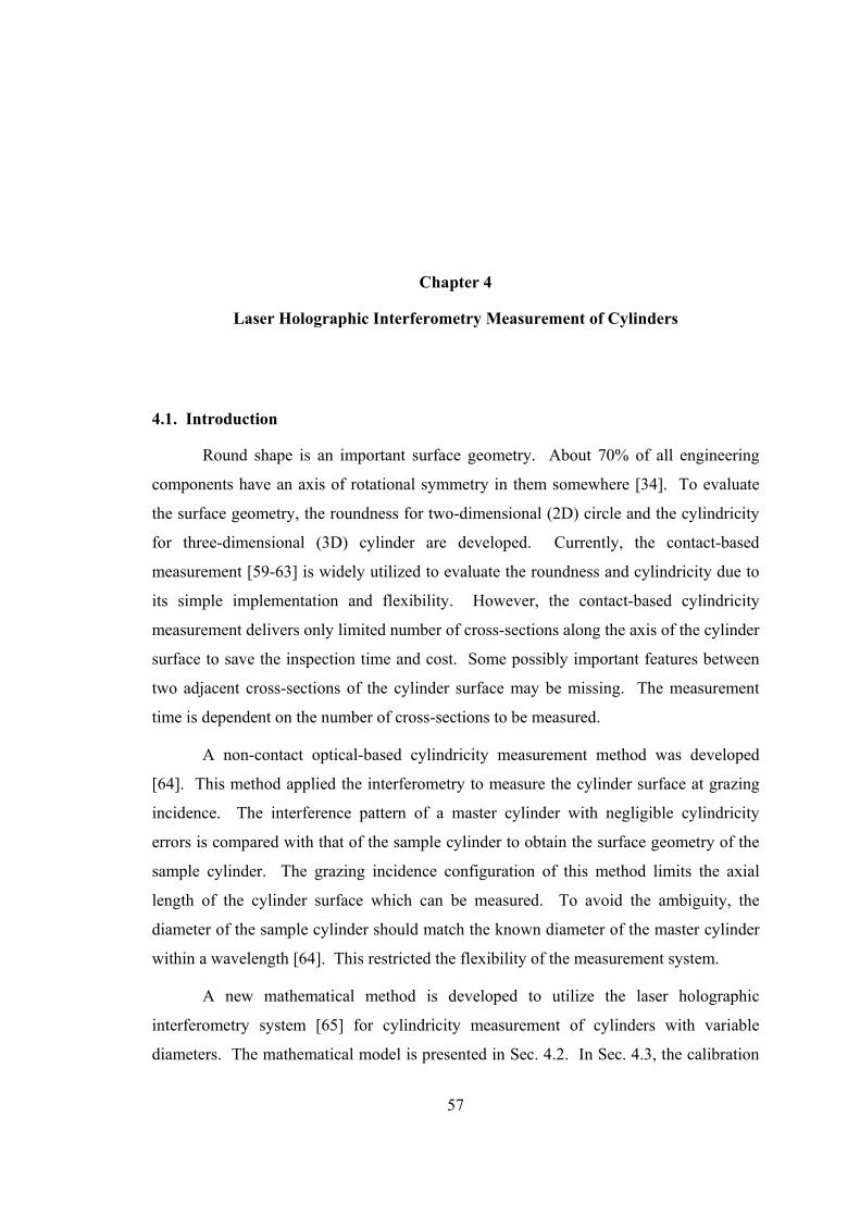
57
Chapter 4
Laser Holographic Interferometry Measurement of Cylinders
4.1. Introduction
Round shape is an important surface geometry. About 70% of all engineering
components have an axis of rotational symmetry in them somewhere [34]. To evaluate
the surface geometry, the roundness for two-dimensional (2D) circle and the cylindricity
for three-dimensional (3D) cylinder are developed. Currently, the contact-based
measurement [59-63] is widely utilized to evaluate the roundness and cylindricity due to
its simple implementation and flexibility. However, the contact-based cylindricity
measurement delivers only limited number of cross-sections along the axis of the cylinder
surface to save the inspection time and cost. Some possibly important features between
two adjacent cross-sections of the cylinder surface may be missing. The measurement
time is dependent on the number of cross-sections to be measured.
A non-contact optical-based cylindricity measurement method was developed
[64]. This method applied the interferometry to measure the cylinder surface at grazing
incidence. The interference pattern of a master cylinder with negligible cylindricity
errors is compared with that of the sample cylinder to obtain the surface geometry of the
sample cylinder. The grazing incidence configuration of this method limits the axial
length of the cylinder surface which can be measured. To avoid the ambiguity, the
diameter of the sample cylinder should match the known diameter of the master cylinder
within a wavelength [64]. This restricted the flexibility of the measurement system.
A new mathematical method is developed to utilize the laser holographic
interferometry system [65] for cylindricity measurement of cylinders with variable
diameters. The mathematical model is presented in Sec. 4.2. In Sec. 4.3, the calibration

58
process is discussed. Simulations and experiment are conducted to demonstrate the
feasibility of the developed method in Sec. 4.4.
4.2. Mathematical model
The mathematical model is based on the customized design of a laser holographic
interferometry system. This model transforms the measurement data from the laser
holographic interferometry into the 3D Cartesian representation of the cylinder surface.
The cylindricity of the cylinder surface is then evaluated.
4.2.1. System design
The regular laser holographic interferometry system for the flat object
measurement is shown in Fig. 4.1(a). This system, which can successfully measure the
flat surfaces of machined metals with µm-level accuracy [65], is composed of three major
components, the vibration isolated table, the optical measurement unit, and the off-axis
parabolic mirror. The vibration isolated table supports the optical measurement unit and
the measurement object. The diverging light coming from the optical measurement unit
is collimated by the parabolic mirror and directed to the measurement object directly.
The light reflected from the measurement object carries the height information of the
object, interferes with the reference light in the optical measurement unit, and generates
the interference pattern. Fourier transformation [65] is applied to analyze the interference
pattern and the 3D surface profile of the flat measurement object is generated.
A cylindrical lens, as shown in Fig. 4.1(b), is applied to customize the optical
system for the cylindricity measurement. Without the cylindrical lens, small amount of
the collimated light coming down from the parabolic mirror can be reflected back from
the round object surface due to the large surface curvature. An ideal cylindrical lens
changes the incident parallel light beam into a converging beam and focuses at a straight
line. With this cylindrical lens, a cylinder can be positioned with the center axis very
close to the focus line of the cylindrical lens as shown in Fig. 4.1(b). The converging
light beam from the cylindrical lens hits the cylinder surface in the direction close to
59
normal and is reflected back through the cylindrical lens to convert into parallel light
beam again. The converted parallel light beam after the cylindrical lens follows the same
path as for the flat surface to generate the interference pattern in the optical measurement
unit.
The cylindrical lens virtually converts the cylindrical surface into flat shape. To
the optical measurement unit, the cylindrical measurement object is still flat. The same
Fourier transformation described above is applied and the calculated value of each
measured point relates to the distance from the corresponding point on the cylindrical
measurement object surface to the focus line of the cylindrical lens.
Only a section of the whole circumference of the cylindrical surface can be
covered in each measurement with the cylindrical lens configured as shown in Fig. 4.1(b).
A rotational stage will be used to hold the cylinder and precisely change its angular
positions. The developed mathematical model is applied to convert the measurement
data from the laser holographic interferometry into the 3D Cartesian representation of the
cylindrical measurement object surface.
4.2.2. Mathematical deduction
The geometric relations between the cylindrical lens, the rotational stage, and the
cylinder are defined in the mathematical model. The format of the measurement data by
the laser holographic interferometry is described. The mathematical transformation is
derived to convert the measurement data into 3D Cartesian representation of the cylinder
surface.
4.2.2.1. Geometric relation definition
The 3D positions of the cylindrical lens focus line, the rotational stage center axis,
and the cylinder center axis do not match in practice. Figure 4.2 is a 3D illustration of the
geometric relations in this configuration. The positions are referred to a common
Cartesian coordinate system with the origin at O(0, 0, 0). This coordinate system is
predefined by the laser holographic interferometry measurement system. The center axis
of the rotational stage goes through the point denoted as O0(x0, y0, z0) and follows the

60
direction denoted as D0(a0, b0, c0). The cylinder center goes through the point denoted as
O1(x1, y1, z1) and follows the direction denoted as D1(a1, b1, c1). As the rotational stage
rotates the cylinder, the position of O1(x1, y1, z1) and the direction D1(a1, b1, c1) will
change. The focus line of the cylindrical lens goes through the point denoted as O2(x2, y2,
z2) and follows the direction denoted as D2(a2, b2, c2). The focal length of the cylindrical
lens is R0.
The collimated light travels down and reaches the cylindrical lens, which converts
the collimated light into converging light. The converging light, which virtually focuses
at a line going through the point O2 and following the direction D2, reaches the cylinder
and covers the region on the cylinder surface marked by hexagons in Fig. 4.2. The
reflected light from the cylinder surface travels through the cylindrical lens and converts
into collimated light to generate the interference pattern in the optical measurement unit
for calculation of “height,” which relates to the distance from the cylinder surface to the
focus line of the cylindrical lens.
It is assumed that the true values of the parameters O1(x1, y1, z1), D1(a1, b1, c1),
O2(x2, y2, z2), D2(a2, b2, c2), and R0 are known for the conversion of measurement data. In
Sec. 4.3, the calibration process is elaborated to estimate these values.
4.2.2.2. Format of measurement data
The measurement data from the laser holographic interferometry system is
delivered in a matrix. For flat surface measurement, the row and column positions of
each element in the matrix linearly correspond to the x and y coordinates of the point on
the object surface, respectively. The value of each element in the matrix indicates the
height of the corresponding point on the object surface. The heights of all the data points
are measured relative to a reference point, which has the height value equal to zero in the
matrix.
For the cylindricity measurement with the configurations shown in Fig. 4.2, the
row and column positions of each element in the matrix correspond to the x and y
coordinates of the point on the cylindrical lens. The value of each element in the matrix
indicates the distance from the point on the cylinder to the focus line of the cylindrical

61
lens minus a constant shift, denoted as S. This constant shift S is the distance from the
reference point, denoted as Pr, to the focus line of the cylindrical lens. In the matrix, the
value of the reference point is zero.
4.2.2.3. Data conversion
The measurement data of a cylinder from the laser holographic interferometry
should be converted into Cartesian form to represent a 3D cylinder surface and calculate
the cylindricity.
The conversion is composed of three steps. First, the point on the focus line of
the cylindrical lens and the optical path, which relates to an element in the measurement
matrix, is calculated. For example, the point Pm on the cylindrical lens, as shown in Fig.
4.2, has the coordinates (xm, ym, zm), in which xm and ym can be calculated from the row
and column positions of the corresponding element in the measurement matrix. The
collimated light reaches Pm and follows the illustrated path to reach the point Po with the
coordinate (xo, yo, zo) on the cylinder. This path virtually converges to the point Pc with
the coordinate (xc, yc, zc) on the focus line of the cylindrical lens. With the (xm, ym) data
of the point Pm, the known focal length R0 of the cylindrical lens, the point O2 (x2, y2, z2),
and the direction D2 (a2, b2, c2), the 3D coordinate of the point Pc and the direction vector
from Pc to Pm can be determined. Second, the relative 3D coordinates of the point Po on
the cylinder surface is calculated with the value, denoted as d0, of the element in the
measurement matrix corresponding to the point Pm, the known constant shift S, and the
calculated 3D coordinate of the point Pc. Third, the calculated 3D coordinate of the point
Po is rotated about the center axis of the rotational stage with the angular position of the
cylinder to compensate its angular position change in different measurements.
The point Pc (xc, yc, zc) on the focus line of the cylindrical lens is determined by:
⎪⎩
⎪⎨
⎧
+=+=+=
tczztbyytaxx
c
c
c
22
22
22
(4.1)

62
where t is the scalar parameter to be determined.
The distance from the point Pc on the focus line of the cylindrical lens to the point
Pm on the cylindrical lens is R0. This relation is expressed by
( ) ( ) ( ) 20
222 Rzzyyxx cmcmcm =−+−+− (4.2)
The direction from the point Pc to Pm is perpendicular to the direction of the focus
line of the cylindrical lens. This relation is expressed by
( ) ( ) ( ) 0222 =−+−+− cmcmcm zzcyybxxa (4.3)
Combine Eqs. (4.1)-(4.3) and a two-degree equation of t is formulated:
[ ]( )( ) ( ) ( )[ ]
( ) ( ) ( )[ ] 0
2
2
22
22
22
22
22
20
2222222
2222
2222222222
22
22
22
22
22
22
22
22
42
42
2
=−+−+−−−+
+−−−−−−++
+++++
cyycxxcRbyaxbyax
cbyycaxxbyaxbyaxbat
cbcababat
mmmm
mmmm (4.4)
The coefficients of t in each term of Eq. (4.4) are known or measurable and Eq.
(4.4) can be solved. There are two roots to the Eq. (4.4). The larger root is always
selected with the assumption that the point O2 is on the beginning side of the cylinder in
the direction of D2.
With the calculated solution to t, the coordinate of the point Pc is calculated using
Eq. (4.1) and the zm coordinate of the point Pm is calculated using Eq. (4.3).

63
The element, corresponding to the point Pm on the cylindrical lens, in the
measurement matrix has the value do. The do plus the constant shift S is the distance from
the point Po to the point Pc. The 3D coordinate of the point Po is calculated by
( )Sdocm
cmco +
−−
+=PPPPPP (4.5)
As the rotational stage rotates the cylinder, the center of the rotational stage and
the focus line of the cylindrical lens are stationary, but the center of the cylinder changes
and the measured surface region on the cylinder is different.
The rotation is conducted to compensate the angular position change of the
cylinder. In practice, the cylinder rotates about the rotational stage center and the
cylindrical lens is fixed. In the model, the cylinder is assumed fixed and the cylindrical
lens is rotated reversely about the center axis of the rotational stage. This assumption
does not change the calculated 3D representation of the cylinder surface because the
movement is relative. Let θ be the angular position of the cylinder, –θ is the angular
position of the cylindrical lens about the center axis of the rotational stage. The
transformation about the center axis of the rotational stage is defined by [66]
( ) ( )( )( ) ( ) )sin()cos(1)cos( 2222222 θθθ −−×+−−−⋅+−−+= OPDOPDDOPOP oooTo
(4.6)
where ToP is the coordinate of the point Po after the transformation by angular rotation –θ
about the center axis of the rotational stage.
Each element in the measurement matrix at every angular position of the cylinder
is converted using the method described above to reach the 3D coordinate ToP . All the
converted ToP form a 3D discrete representation of the cylinder surface in the Cartesian

64
coordinate system. Based on this 3D representation, the cylindricity of the cylinder can
be evaluated.
4.2.3. Cylindricity evaluation
Many cylindricity evaluation methods, based on least square and minimum zone
[67-70], have been developed. The least square evaluation with Gauss-Newton iteration
is applied to estimate the cylindricity because the estimated reference cylinder using this
method is unique and robust to a few isolated noisy points [34]. The reference cylinder,
from which the deviations of all the measured points are determined, should be identified
to calculate the cylindricity. The cylindricity is defined as the range of the deviations of
all the measured points from the reference cylinder. This cylindricity evaluation method
starts with an initial guess of the reference cylinder and conducts iterations until the
estimation of the reference cylinder (radius and position of center axis) converges within
a predefined error.
Some transformations of the data points are conducted at the beginning of each
iteration to simplify the process. The data points are translated and rotated at the
beginning of each iteration to make the trial reference cylinder of this iteration have its
center axis lie on the y axis. The Jacobian matrix is calculated to identify the incremental
step for each parameter estimate. Update the parameter estimates for the next iteration by
adding the incremental step to each parameter with the reverse transformations.
The translation and rotation are conducted to make the center axis of the reference
cylinder lie on the y axis.
The translation of the data points is achieved by:
⎟⎟⎟
⎠
⎞
⎜⎜⎜
⎝
⎛−
⎟⎟⎟
⎠
⎞
⎜⎜⎜
⎝
⎛=
⎟⎟⎟
⎠
⎞
⎜⎜⎜
⎝
⎛
1
1
1
:zyx
zyx
zyx
oi
oi
oi
oi
oi
oi
(4.7)
where

65
the operator := means update the parameters on the left side,
i is the number of converted points TP io, , i = 1,2,…, N, and
N is the total number of measured points.
The rotation of the data points is achieved by:
⎟⎟⎟
⎠
⎞
⎜⎜⎜
⎝
⎛=
⎟⎟⎟
⎠
⎞
⎜⎜⎜
⎝
⎛
oi
oi
oi
oi
oi
oi
zyx
zyx
U: (4.8)
where
U is the rotation matrix ⎟⎟⎟
⎠
⎞
⎜⎜⎜
⎝
⎛−
⎟⎟⎟
⎠
⎞
⎜⎜⎜
⎝
⎛
−=
1000cossin0sincos
cossin0sincos0
001
11
11
22
22 θθθθ
θθθθU ,
θ1 is the angle to be rotated around the z axis, and
θ2 is the angle to be rotated around the x axis.
The angles θ1 and θ2 are determined by the condition:
⎟⎟⎟
⎠
⎞
⎜⎜⎜
⎝
⎛=
⎟⎟⎟
⎠
⎞
⎜⎜⎜
⎝
⎛
010
1
1
1
cba
U (4.9)
Eq. (4.9) defines the transformation which makes the direction D1(a1, b1, c1) of
the center axis of the cylinder parallel to the y axis (0, 0, 1).

66
The data points can be reversely transformed by:
⎟⎟⎟
⎠
⎞
⎜⎜⎜
⎝
⎛+
⎟⎟⎟
⎠
⎞
⎜⎜⎜
⎝
⎛=
⎟⎟⎟
⎠
⎞
⎜⎜⎜
⎝
⎛
1
1
1
:zyx
zyx
zyx
oi
oi
oi
oi
oi
oiTU (4.10)
where UT is the transpose of the matrix U.
To identify the incremental step of each parameter estimate for next iteration, the
Jocobian matrix is calculated by
J =
⎟⎟⎟⎟⎟
⎠
⎞
⎜⎜⎜⎜⎜
⎝
⎛
∂∂
∂∂
∂∂
∂∂
∂∂
∂∂
∂∂
∂∂
∂∂
∂∂
11111
1
1
1
1
1
1
1
1
1
1
...
Rq
cq
aq
zq
xq
rq
cq
aq
zq
xq
nnnnn
(4.11)
where
1Rrq ii −= , (4.12)
[ ][ ][ ]
( ) 2/121
21
21
2/1
21111
21111
21111
)()(
)()(
)()(
cba
yyaxxb
xxczza
zzbyyc
r
oioi
oioi
oioi
i ++
⎪⎪⎭
⎪⎪⎬
⎫
⎪⎪⎩
⎪⎪⎨
⎧
−−−
+−−−
+−−−
= , (4.13)
R1 is the radius of the reference cylinder.
With the center axis of the reference cylinder lie on the y axis, a1 = 0, b1 = 1, c1 =
0, x1 = 0, and y1 = 0. Eq. (4.13) can be simplified as

67
22oioii zxr += (4.14)
And each element in the Jacobian matrix J, described in Eq. (4.11), can have a
significantly simplified expression:
i
oii
rx
xq
−=∂∂
1
,
i
oii
rz
zq
−=∂∂
1
,
i
oioii
ryx
aq
−=∂∂
1
, (4.15)
i
oioii
rzy
cq
−=∂∂
1
,
11
−=∂∂Rqi .
The incremental steps of the parameter estimates are determined by
( )⎟⎟⎟
⎠
⎞
⎜⎜⎜
⎝
⎛
−
−=
⎟⎟⎟⎟⎟⎟
⎠
⎞
⎜⎜⎜⎜⎜⎜
⎝
⎛
−
n
R
c
a
z
x
q
q
IIIII
...1
1
1
1
1
1
1
JJT (4.16)
The parameter estimates are updated by

68
⎟⎟⎟
⎠
⎞
⎜⎜⎜
⎝
⎛
−−+⎟⎟⎟
⎠
⎞
⎜⎜⎜
⎝
⎛=
⎟⎟⎟
⎠
⎞
⎜⎜⎜
⎝
⎛
1
1111
1
1
1
1
1
1
1
:
z
czbx
x
IIIII
I
zyx
zyx
TU ,
⎟⎟⎟
⎠
⎞
⎜⎜⎜
⎝
⎛
=⎟⎟⎟
⎠
⎞
⎜⎜⎜
⎝
⎛
1
1
1:
1
1
1
c
a
I
I
cba
TU , and (4.17)
111 : RIRR += .
4.2.4. Registration adjustment
The registration adjustment is developed to reduce the effect of parameter
estimate errors on the cylindricity evaluation. In the process described above, the true
values of all the parameters are assumed to be known. In practice, these values have to
be estimated or measured with some errors. The registration adjustment is applied before
the cylindricity calculation of the whole cylinder to transform the converted 3D data
points of each measurement so that the center axis of the reference cylinders of all the
measurements match with each other.
The center axis of the fitted cylinder of each measurement is estimated using the
cylindricity calculation iteration process described in Sec. 4.2.3. For example, the center
point and the direction of the center axis are estimated as O1k and D1k for measurement k.
The means of O1k and D1k, denoted as 1O and 1D , respectively, are the target axis
position for all the measurements. The transformation of the data points for each
measurement is determined by
11 OOT +⎟⎟⎟
⎠
⎞
⎜⎜⎜
⎝
⎛−
⎟⎟⎟
⎠
⎞
⎜⎜⎜
⎝
⎛=
⎟⎟⎟
⎠
⎞
⎜⎜⎜
⎝
⎛
oi
oi
oi
oi
oi
oi
zyx
zyx
(4.18)

69
where Ti is the rotation matrix determined by kk 11 DTD = .
4.3. Calibrations
Calibrations are conducted to estimate the position of the rotational stage center
axis, the position of the focus line of the cylindrical lens, the focal length of the
cylindrical lens, and the constant shift of the reference point, which are assumed to be
known in the mathematical model described in Sec. 4.2.
A master cylinder with known radius and negligible cylindricity errors is used for
the calibrations. The cylindricity of the master cylinder is calculated using the
mathematical model described in Sec. 4.2 with the initial guess of all the parameters to be
estimated. Within the possible range of all the parameters to be estimated, iterations are
conducted to find an optimal combination of these parameters, which deliver the
minimum cylindricity error. This optimal combination of these parameters will be used
for the mathematical model. Multiple randomly-selected initial guess combinations of
the parameters are used to reduce the sensitivity of the converged results to the initial
guess.
The computational time of this calibration may be long but this is a one-time
process and can be implemented offline. Once all the parameters are calibrated, the
master cylinder is released. Without changing the relative locations between the
rotational stage and the cylindrical lens, a sample cylinder with variable diameters is
fixed. It is important to note that the center of the sample cylinder does not have to be
maintained same as the master cylinder. Centering and leveling of the sample cylinder
on the chuck of the rotational stage will only change the center axis of the sample
cylinder, not the rotational stage center axis.
4.4. Examples
Simulations and an experiment are conducted to demonstrate the developed
mathematical model.

70
4.4.1. Simulations
Three simulations, one for the cylindricity measurement, one for the calibration
process, and the other for the error analysis, are conducted.
4.4.1.1. Cylindricity measurement
The simulation for the cylindricity measurement assumes that the true values of
the position of the center axis of the rotational stage, the position of the focus line of the
cylindrical lens, the focal length of the cylindrical lens, and the constant shift of the
reference point, are known. The laser holographic interferometry measurements at
different angular positions of a perfect cylinder are simulated excluding any measurement
errors. These simulated measurement results are input to the developed algorithm and the
cylindricity of the cylinder is calculated. By comparing the calculated cylindricity with
the true cylindricity (= 0), the algorithm is evaluated.
The true values of the following parameters are assumed. The coordinate of point
O0 which the center axis of the rotational stage goes through is O0 = (0, 0, 0.5) mm. The
direction D0 which the center axis of the rotational stage follows is D0 = (0, 1, 0). The
coordinate of point O1 which the center axis of the cylinder goes through at the angular
position of 0º is O1 = (0, 0, 1) mm. The direction D1 which the center axis of the cylinder
follows at the angular position of 0º is D1 = (0, 0.9988, 0.0499). The coordinate of point
O2 which the center axis of the converging light goes through is O2 = (0, 0, –1) mm. The
direction D2 which the center axis of the converging light follows is D2 = (0.0995, 0.9950,
0). The focal length R0 of the cylindrical lens is 50 mm. The radius R of the perfect
cylinder is R = 12.5 mm. The constant shift S of the reference point is assumed to be S =
12 mm. For each measurement, the angular and axial coverage of the cylinder surface
are 90º and 15 mm, respectively. The covered region of the cylinder surface in each
measurement is represented by a measurement matrix with the dimension of 128 x 128.
Four rotations with an angular incremental step of 90º are simulated.
The 3D illustrations of the four simulated measurement matrices from the laser
holographic interferometry system are shown in Fig. 4.3 with the sampling rate of every 8

71
points for the purpose of easy illustration. The angular positions of the four
measurements in Figs. 4.3(a) to 4.3(d) are 0º, 90º, 180º, and 270º, respectively. The black
dots correspond to elements in the measurement matrix. The lines connecting the dots
indicate the rows, which correspond to the direction closely perpendicular to the cylinder
axis, in the measurement matrix. Irregular shapes of the simulated measurements are
observed and these shapes change as the angular position of the cylinder changes. This is
because center axes of the cylinder, the rotational stage, and the cylindrical lens do not
match in 3D space. Ideally, if these three center axes match, the measurement matrix will
appear as the same flat plane at different angular positions.
These four simulated measurement matrices and the corresponding angular
positions of the cylinder are input to the cylindricity measurement program, which has
the true values of the O0, D0, O2, D2, R0, and S. Using the mathematical model described
in Sec. 4.2, the 3D surface profile of the cylinder is generated, as shown in Fig. 4.4. A
mismatch is observed in the connecting regions between two adjacent sets of the
converted 3D measurement data points. This is because that the center axis of the
rotational stage and the focus line of the cylindrical lens do not match. However, this
mismatch does not impact the estimated cylindricity because all the converted data points
are still on the same cylinder surface. The estimated cylindricity using the evaluation
algorithm in Sec. 4.2.3 is 1.24 × 10 –14 mm. Compared with the true value (= 0 mm), the
algorithm is validated.
4.4.1.2. Calibration
The same four simulated measurement matrices and the corresponding angular
positions as in Sec. 4.4.1.1 are input to the calibration program. However, the program
does not have the information of the true values for the parameters: O0, D0, O2, D2, R0,
and S. The iteration process, described in Sec. 4.3, is applied to estimate these values. In
practice, these estimated values will be used as the true values for the cylindricity
calculation.
After totally 18,042 iterations for 10 min in MATLAB 7.0 on a standard PC, the
final estimated parameters are O0 = (–2.9694×10⁻⁵, 0, –0.3718) mm, D0 = (1.5568×10⁻⁸,

72
1, –3.4482×10⁻⁹), O2 = (–3.1332×10⁻⁵, 0, –1.8718) mm, D2 = (0.099504, 0.99504, –
4.0115×10⁻⁸), R0 = 50.000 mm, and S = 12.001 mm, which delivers the cylindricity as
7.8741×10⁻⁷ mm. The estimated cylindricity converges to the true value (0 for a perfect
cylinder) within the error smaller than 0.001 µm. Those estimated parameters also
converge very closely to the true values except the positions of O0 and O2. However, the
relative position between the estimated O0 and O2 is (1.7693×10⁻⁵, 0, –1.5000) mm,
which is very close to the true relative position, which is (0, 0, –1.5) mm, between O0 and
O2. This is because wherever the center axis of the rotational stage and the focus line of
the cylindrical lens are located, the generated cylinder surface profile will be the same if
the relative position between the center axis of the rotational stage and the focus line of
the cylindrical lens keeps the same. These results demonstrate the convergence and
feasibility of developed mathematical model.
4.4.1.3. Error analysis
The cylindricity measurement error is analyzed by considering the parameter
estimation errors in the cylindrical lens, the rotational stage, and the measurement system
with the assumption that the cylindrical lens is ideal, i.e., there is no aberration to disable
the cylindrical lens to focus at a straight line.
The parameter estimation errors in the cylindrical lens include the focal length
error ∆R0, the point position error ∆O2(∆x2, ∆y2, ∆z2), the direction error ∆D2(∆a2, ∆b2,
∆c2) in which only two parameters are independent, and the constant shift error ∆S. The
rotational stage error is the angular position error ∆θ. The measurement system errors
include the lateral position errors ∆xm and ∆ym, and the height measurement error ∆do.
The errors of these parameters are assumed to follow the normal distribution with a
reasonable deviation. The true values of all the parameters are also assumed known.
The cylindricity measurement error is analyzed in two steps. First, the error of
each parameter is applied separately with all the other parameters equal to true value to
quantify the sensitivity of the cylindricity measurement error using the Eqs. (4.1)-(4.6).
Due to the complexity of the equations, explicit expression of the sensitivity is not
derived. The true value plus error is input directly to the cylindricity calculation program

73
to calculate the cylindricity error. Second, Monte Carlo simulation is conducted with the
effects of all the parameters errors included simultaneously in the cylindricity
measurement. The error of each parameter is assumed to follow the normal distribution.
The true values of these parameters are assumed to be the same as in Sec. 4.4.1.1.
The errors of each parameter are assumed to follow the normal distribution with the
expected value equal to 0. The 3σ of these parameters are: ∆R0 = 0.010 mm, ∆O2 is
within a sphere of 0.010 mm radius centered at the true position O2, ∆D2 is within 0.05º
range from the true direction D2, ∆S = 0.010 mm, ∆xm = 0.15 mm, ∆ym = 0.15 mm, ∆d0 =
1 µm, and ∆θ = 0.04º.
The effect of each parameter error on the final cylindricity measurement is shown
in Table 4.1. The first set of the cylindricity error is due to the effect of the parameter
estimation error of the cylindrical lens. With the error of each parameter (3σ) listed in
Table 4.1, the corresponding cylindricity measurement errors before and after the
registration adjustment are recorded. The registration adjustment can significantly reduce
the cylindricity measurement error induced by the cylindrical lens parameter estimation
errors, except the position estimation error ∆O2. This is because position error ∆O2
makes the converted 3D representation out of the cylindrical shape and this error cannot
be rectified by adjusting the measurement data to match the reference cylinder of
different measurements. The 0.05º ∆D2 error makes one end of the focus line 0.079 mm
away from the true position for a 45 mm long cylinder, which is used in the simulation.
After converting the error to the same scale, it is observed that the cylindricity
measurement error is most sensitive to position estimation error ∆O2 of the point on the
focus line. Only 0.010 mm ∆O2 introduces 0.030 mm cylindricity measurement error.
The other two sets of Table 4.1 are the effects of the system measurement error
and the rotational stage error. The 0.15 mm ∆xm and ∆ym are the lateral resolution of the
laser holographic interferometry system. The 1 µm ∆d0 is the height measurement
accuracy of the system. The 0.04º ∆θ is the calibrated accuracy of the rotational stage
used in this research. The registration adjustment does not affect any effect of the system
measurement error or the rotational stage error because these two kinds of errors change
the position of the measured data points symmetrically about the center axis. The lateral

74
position error of the system has an important effect on the cylindricity measurement. The
height measurement error of the system is linearly mapped to the cylindricity
measurement error. The effect of the angular positioning error of the rotational stage on
the cylindricity measurement is trivial.
The Monte Carlo simulation is conducted to include all the error effects
simultaneously and investigate the performance of the cylindricity measurement. The
same parameter estimation errors listed in Table 4.1 are used and 1000 simulations are
conducted. The histogram of the simulated cylindricity measurement error after the
registration adjustment is shown in Fig. 4.5. The minimum cylindricity measurement
error is 0.024 mm. The mean and standard deviation of the cylindricity measurement
error are 0.097 mm and 0.054 mm, respectively.
4.4.2. Experiment
This experiment applies the Coherix Shapix 2000 laser holographic
interferometry system with a cylindrical lens, the rotational stage, and a fine adjustment
mechanism to measure a centerless ground steel cylinder. The system configurations, the
experiment procedures, the measurement results, and the processing are elaborated.
4.4.2.1. System configurations
The system configuration of the cylindricity measurement experiment is shown in
Fig. 4.6. All the components are inside the measurement cabinet of the laser holographic
interferometry system. The rotational stage HAAS HA5C is fixed on the vibration
isolated table. A centerless ground steel cylinder (25.4 mm in diameter) is used as a
master cylinder to verify the developed mathematical model. The master cylinder is
fixed in the chuck, which is attached to the rotational stage. There are 4 centering screws
(only 2 visible in Fig. 4.6), positioned at 0º, 90º, 180º, and 270º around the circumference
of the chuck to adjust the center position of the master cylinder. The cylindrical lens,
which is bonded to the fine adjustment mechanism with 4 degrees of freedom, is

75
positioned above the master cylinder. A granite plate is positioned beside the master
cylinder. This granite plate, used as a height datum, is fixed through the whole
measurement process and measured with the laser going down directly to the surface.
4.4.2.2. Adjustments
Adjustment is conducted before the measurement. Three components, the master
cylinder, the cylindrical lens, and the granite plate, are adjusted in sequence.
The master cylinder is centered after it is fixed in the chuck. This centering is
conducted by adjusting the four centering screws on the chuck with a dial indicator in
contact with the master cylinder surface. The runout of the master cylinder after
centering is less than 25 µm.
The cylindrical lens is adjusted by the fine adjustment mechanism to have good
modulations at 0º, 90º, 180º, and 270º positions. The mechanism has four degrees of
freedom: translation in x direction, translation in z direction, rotation about x axis, and
rotation about z axis.
The orientations of the granite plate are adjusted by the three adjustment screws
underneath to have good surface reflectivity. This granite plate is fixed after the
adjustment and used as a height datum. This will be elaborated in Sec. 4.4.2.4.
After the adjustment, measurement of the cylinder surface and the granite plate is
conducted in one image capturing. Between two consecutive measurements, the
rotational stage is rotated by inputting an angle value on the control panel with the
resolution of 0.001º.
4.4.2.3. Measurement results
The surface area covered in one measurement is about 9º of the cylinder and
about 42 mm axial length. Each measurement contains more than 20,000 points. Totally
there are 58 measurements, which add up to more than 1 million points.
Figures 4.7 to 4.10 show four typical height measurement results obtained by
Coherix Shapix 2000 system. The angular positions of these four measurements are

76
333.140º, 62.227º, 149.988º, and 244.377º, respectively, with about 90º spacing. Fig.
4.7(a) is a 2D grayscale illustration of the measurement matrix. The left rectangle
corresponds to the master cylinder surface. The right rectangle is for the granite plate.
Two lines, Line 1 from –y to +y and Line 2 from –x to +x, are drawn across the grayscale
map in Fig. 4.7(a). The height profiles along these two lines are illustrated in Figs. 4.7(b)
and 4.7(c), respectively. These two lines are drawn at the same positions in Figs. 4.8(a),
4.9(a), and 4.10(a) as in Fig. 4.7(a). Compare the profiles at these four angular positions
along Line 1 and Line 2, respectively, it is observed that at angular positions of 333.140º
and 244.377º, the trend of the master cylinder surface leans upward from –y to +y;
whereas the trend at the angular positions of 62.227º and 149.988º is opposite. This
indicates that the center axis of the rotational stage and the center axis of the cylinder do
not match in the 3D space. The height positions of the granite plate change between the
four angular positions. This is because the reference point, which has the height value
equal to 0 in the measurement matrix, changes as the cylinder rotates. The trend of Line
2 at the angular positions of 333.140º and 62.227º leans downward from –x to +x;
whereas the trend at the angular positions of 149.988º and 244.377º is opposite.
4.4.2.4. Processing
The height measurement data of the master cylinder from the 58 measurements
are first adjusted with reference to the height measurement data of the granite plate,
which is fixed through the whole measurement process and used as common height
datum. The reason of this adjustment is that the Coherix Shapix measurement is relative,
i.e., all the height data points in one measurement are relative to a reference point, and
this reference point changes as the master cylinder rotates. The measured height of the
granite plate from all the measurements is compared with the first measurement. The
difference of height is least square fitted by a plane and the trend of this plane will be
subtracted from the corresponding height measurement data of the master cylinder.
The row and column coordinates of the element in the height matrix of the
Coherix Shapix 2000 measurement are converted into the x and y coordinates. All the 58
adjusted and converted measurement data of the master cylinder together with the
77
corresponding angular positions are input to the program. Initial guess are generated to
estimate O0, D0, O2, D2, R0, and S. Then iterations are conducted to find the optimal
values of these unknown parameters, which deliver the minimum cylindricity error of the
master cylinder. To avoid the problem of iteration sensitivity to initial guess, multiple
initial guess of the randomly selected unknown parameters are used.
The converged solution is reached after 4568 iterations for more than 33 hours.
Figure 4.11 shows the generated 3D surface profile of the master cylinder surface with
the final estimation of these parameters. The estimated values of all the unknown
parameters are: O0 = (160.3313, 0, –12.4622) mm, D0 = (–0.1369, 0.9796, –0.1469), O2 =
(162.1639, 0, –14.2365) mm, D2 = (–0.1467, 0.9783, –0.1466), R0 = 251.12 mm, and S =
123.22 mm, which delivers the cylindricity error as 123 µm.
The master cylinder was measured by the contact-based Taylor Hobson TalyRond
265 system. The cylindricity of the same surface region was 8 µm with 2 mm spacing
between two adjacent cross-sections of the cylinder. Compared with this contact-based
measurement result, a 115 µm error in the laser holographic interferometry measurement
exists. There are four possible reasons for this error. First, the possible runout error of
the rotational stage may have a significant effect on the cylindricity evaluation. Second,
the measurement data from the laser holographic interferometry system is not rectified
and some significant errors in the lateral coordinates x and y may exist. Third, the
iteration process to estimate the system configuration parameters may not find the
globally optimal combination. Fourth, the cylindrical lens used in this research is off-the-
shelf and some significant aberrations of the cylindrical lens may exist. A calibration
process of the cylindrical lens shall be developed.
Different error sources are quantified to analyze their contributions to the 115 µm
cylindricity measurement error. The maximum runout error of the rotational stage, which
is used in this research, is the 10 µm [71]. This indicates that the center axis of the
rotational stage should be within a virtual 10 µm radius cylinder centered at a stationary
and perfect straight line. The maximum cylindricity measurement error introduced by the
10 µm runout of the rotational stage is 20 µm. The lateral coordinate measurement errors
∆xm (= 0.15 mm) and ∆ym (= 0.15 mm) of the laser holographic interferometry system

78
will have the cylindricity measurement errors equal to 15 µm and 29 µm, respectively, as
shown in Table 4.1. The 1 µm height measurement accuracy of the laser holographic
interferometry will generate the 2 µm cylindricity measurement error. The total error
contribution of the laser holographic interferometry is 46 µm. The iteration process
described in Sec. 4.3 can also have some system parameter estimation errors. Assume
the system parameter estimation errors are ∆R0 = 10 µm, ∆S = 10 µm, and ∆O2 = 10 µm,
the cylindricity measurement errors introduced by these errors are calculated using the
Eqs. (4.1)-(4.6) as 0.8 µm, 0.4 µm, and 30 µm, respectively. The total error contribution
of these assumed system parameter estimation errors is 31 µm. The aberration of the
cylindrical lens also contributes to the cylindricity measurement error. Assume there is 5
µm error in focusing the light to the focus line of the cylindrical lens. This focusing error
will generate another ∆O2 up to 5 µm for all light directions and introduce up to 15 µm
cylindricity measurement error. These four error contributions, 20 µm by the 10 µm
runout of the rotational stage, 46 µm by the lateral and height measurement errors of the
laser holographic interferometry system, 31 µm by the assumed system parameter
estimation errors ∆R0 = 10 µm, ∆S = 10 µm, and ∆O2 = 10 µm, and 15 µm by the
assumed 5 µm focusing error, add up to about 112 µm cylindricity measurement error.
This quantitatively explains the error sources of the cylindricity measurement. More
experiments shall be conducted to verify the assumed system parameter estimation errors
and evaluate the aberrations of the cylindrical lens.
4.5. Concluding remarks
A mathematical method was developed to utilize the laser holographic
interferometry with customized optical and mechanical configurations for flexible and
full surface measurement of cylinders with variable diameters. A cylindrical lens was
used to customize the optical system and enable the laser holographic interferometry for
the inspection of cylinders. A rotational stage was applied to rotate the cylinder and the
whole circumference of the cylinder can be measured. The developed mathematical
model converted the laser holographic interferometry measurements into the 3D

79
representation of the cylinder surface from which the cylindricity can be calculated. The
simulation demonstrates that the developed method can estimate the system configuration
parameters with good accuracy. The effect of the estimation error of system
configuration parameters and the measurement error on the cylindricity measurement was
analyzed. The experiment with the master cylinder was conducted and the cylindricity
was estimated with an error of 115 µm, which was mainly due to the four possible error
sources.
Two possible future researches can follow. First, this method assumes no
aberration in the cylindrical lens. A calibration procedure of the cylindrical lens should
be developed to accommodate the aberrations of the optical system. Second, a more
robust and time-efficient calibration process should be developed to improve the
performance of the estimation of the unknown parameters.

80
Table 4.1. The cylindricity measurement error due to the parameter estimation errors.
Maximum cylindricity error (mm) Parameter estimation error
(3σ) Before registration adjustment
After registration adjustment
∆R0 = 0.010 mm 0.002 0.001
∆O2 = 0.010 mm 0.029 0.030
∆D2 = 0.05º 0.043 0.010
∆S = 0.010 mm 0.0008 0.0004
∆xm = 0.15 mm 0.015 0.015
∆ym = 0.15 mm 0.028 0.029
∆d0 = 1 µm 0.002 0.002
∆θ = 0.04º 0.000 0.000

81
Vibration isolated table
Optical measurement unit
Off-axis parabolic mirror
Object
(a)
Vibration isolated table
Optical measurement unit
Off-axis parabolic mirror
Cylinder
Cylindrical lens
(b)
Fig. 4.1. Conceptual system design of the laser holographic interferometry system: (a) flat object measurement and (b) cylindricity measurement.
x
z
x
z

82
Fig. 4.2. 3D illustration of the geometric relations in the mathematical model for the
cylindricity measurement with the laser holographic interferometry system.
x
z
y
O0 O1 O2
Pc
Cylindrical lens
Collimated light
Po
Pm
O
R0
D0 D1 D2
Cylinder
Pr
S

83
-40-30
-20-10
010
2030
40
-50
510
1520-1
0
1
2
3
4
x (mm)y (mm)
z (m
m)
-40-30
-20-10
010
2030
40
-50
510
1520-1
0
1
2
3
4
x (mm)y (mm)
z (m
m)
(a) (b)
-40-30
-20-10
010
2030
40
-50
510
1520-1
0
1
2
3
4
x (mm)y (mm)
z (m
m)
-40
-30-20
-100
1020
3040
-50
510
1520-1
0
1
2
3
4
x (mm)y (mm)
z (m
m)
(c) (d)
Fig. 4.3. 3D illustration of four simulated laser holographic interferometry measurements of the cylinder with O0 = (0, 0, 0.5) mm, D0 = (0, 1, 0), O2 = (0, 0, –1) mm, D2 = (0.0995, 0.9950, 0), R = 12.5 mm, and S = 12 mm (O1 = (0, 0, 1) mm and D1 = (0, 0.9988, 0.0499)
at the 0º angular position of the cylinder): (a) at 0º angular position, (b) at 90º angular position, (c) at the angular position of 180º, and (d) at the angular position of 270º of the
cylinder.

84
-15-10
-50
510
15
-50
510
1520-15
-10
-5
0
5
10
15
x (mm)y (mm)
z (m
m)
Fig. 4.4. Generated cylinder surface profile from the simulated data (cylindricity = 7.9×10⁻⁷ mm).

85
Fig. 4.5. The cylindricity measurement error distribution simulated by the Monte Carlo
method.
0%
2%
4%
6%
8%
10%
12%
0.02 0.05 0.08 0.11 0.14 0.17 0.20 0.23 0.26 0.29 0.32 0.35 0.38Cylindricity Error (mm)

86
Fig. 4.6. System configurations of the cylindricity measurement.
Rotational Stage
Cylindrical Lens
Master Cylinder
Fine Adjustment Mechanism
Granite Plate Centering Screws
y
z
Adjustment Screws
Measurement cabinet of the laser holographic interferometry system

87
(a)
0 20 40 60 80 100 120-0.04
0.01
0.06
0.11
0.16
0.21
(mm)
Hei
ght (
mm
)
0 5 10 15 20 25 30 35 40 45
-0.01
0
0.01
0.02
0.03
0.04
0.05
(mm)
Hei
ght (
mm
)
(b) (c)
Fig. 4.7. Height measurement of the master cylinder at the angular position of 333.140º: (a) 2D color map, (b) height profile along Line1 from left to right in (a), and (c) height
profile along Line 2 from top to bottom in (a).
Master cylinder
Granite PlateLine 1
Line 2
y
x

88
(a)
0 20 40 60 80 100 120-0.04
0.01
0.06
0.11
0.16
0.21
(mm)
Hei
ght (
mm
)
0 5 10 15 20 25 30 35 40 45
-0.01
0
0.01
0.02
0.03
0.04
0.05
(mm)
Hei
ght (
mm
)
(b) (c)
Fig. 4.8. Height measurement of the master cylinder at the angular position of 62.227º: (a) 2D color map, (b) height profile along the Line 1 from left to right in (a), and (c)
height profile along the Line 2 from top to bottom in (a).
Master cylinder
Granite PlateLine 1
Line 2
y
x

89
(a)
0 20 40 60 80 100 120-0.04
0.01
0.06
0.11
0.16
0.21
(mm)
Hei
ght (
mm
)
0 5 10 15 20 25 30 35 40 45
-0.01
0
0.01
0.02
0.03
0.04
0.05
(mm)
Hei
ght (
mm
)
(b) (c)
Fig. 4.9. Height measurement of the master cylinder at the angular position of 149.988º: (a) 2D color map, (b) height profile along the Line 1 from left to right in (a), and (c)
height profile along the Line 2 from top to bottom in (a).
Master cylinder
Granite PlateLine 1
Line 2
y
x

90
(a)
0 20 40 60 80 100 120-0.04
0.01
0.06
0.11
0.16
0.21
(mm)
Hei
ght (
mm
)
0 5 10 15 20 25 30 35 40 45
-0.01
0
0.01
0.02
0.03
0.04
0.05
(mm)
Hei
ght (
mm
)
(b) (c)
Fig. 4.10. Height measurement of the master cylinder at the angular position of 244.377º: (a) 2D color map, (b) height profile along the Line 1 from left to right in (a), and (c)
height profile along the Line 2 from top to bottom in (a).
Master cylinder
Granite PlateLine 1
Line 2
y
x

91
Fig. 4.11. 3D illustration of the final estimation of the master cylinder.

92
Chapter 5
Conclusions and Future Work
5.1. Conclusions
This research developed three new methods to improve the laser holographic
interferometry for the 3D precision and full surface measurement of manufactured
components. The flatness evaluation errors for the high definition measurement system
were investigated.
A hologram registration method without using targets was developed in Chapter 2
for the laser holographic interferometry measurement of objects larger than the field of
view (FOV). The cross-correlation analysis was used to identify the translation and
overlapped regions, which determine the tilt and shift correction for hologram registration.
The proposed method was validated using two examples with different approaches. The
first example, a wheel hub smaller than the FOV, demonstrated only 0.1 µm discrepancy
of the surface flatness between the registered and standard measurements. The second
example, an engine head combustion deck surface, was larger than the FOV. The
registered surface measurements were compared to that of CMM with only 2.5%
discrepancy of the peak-to-valley flatness. This hologram registration method enables
the µm-level precision measurement of large objects.
A phase unwrapping method was developed in Chapter 3 to mathematically
increase the height measurement range of the laser holographic interferometry while
maintaining the same level of accuracy and resolution. Three approaches, including the
masking and recovery, dynamic segmentation, and phase adjustment for pixels in thin
boundary regions, were developed to effectively avoid the divergence problem of

93
boundary pixels. This method successfully solves the phase unwrapping problem of the
laterally discontinuous surfaces and is validated using an example of the automatic
transmission valve body.
A mathematical method was developed in Chapter 4 to utilize the laser
holographic interferometry with customized optical and mechanical configurations for
flexible and full surface measurement of cylinders with variable diameters. The
developed mathematical model converts the laser holographic interferometry
measurements into the 3D representation of the cylinder surface from which cylindricity
was calculated. The simulation demonstrated that the developed method can estimate the
system configuration parameters with good accuracy. The effect of the estimation error
of system configuration parameters and the measurement error on the cylindricity
measurement was analyzed. The experiment was conducted to measure the master
cylinder with negligible cylindricity errors and the feasibility of the developed method
was verified.
A preliminary study was conducted in Appendix C to analyze the flatness
evaluation errors for high definition measurements. Two commonly used methods, least
square and minimum zone, were analyzed in the estimation error of the reference plane
for flatness evaluation. The widely-used peak-to-valley flatness definition and two
proposed flatness definitions, 6σf and modified peak-to-valley, were assessed. Five
surface profiles with the random measurement errors were generated to simulate the
flatness evaluation process. The results showed that the least square method with the
modified peak-to-valley definition has the good potential among the analyzed methods to
effectively evaluate the flatness with good noise robustness for the high definition
measurement system.
5.2. Future work
This research will continue in two areas. First is to further improve the
performance of the cylindricity measurement with the laser holographic interferometry
system. Third is to develop a more comprehensive method to quantitatively evaluate

94
different geometrical form measurement errors for the high definition measurement
system.
5.2.1. Performance improvement of cylindricity measurement
The cylindricity measurement methods developed in Chapter 4 is verified in
simulations to be capable of estimating the system configuration parameters and
evaluating the cylindricity with good accuracy. The conducted experiment demonstrates
the feasibility of this method in practice but the cylindricity evaluation accuracy needs
improvement.
To further improve the performance of the cylindricity measurement, two
research investigations will follow.
• Calibration of cylindrical lens: The cylindrical lens used in Chapter 4 is off-the-shelf
and no calibration was conducted. An aspherical cylindrical lens with minimum
aberrations should be utilized to advance the performance of the method. An
effective calibration method of the cylindrical lens, using a master cylinder with
negligible cylindricity errors and precisely rectified grooves, as shown in Fig. 5.1,
should be developed. The rectified grooves will appear in a possibly distorted way in
the generated 3D representation of the cylinder due to the aberrations of the
cylindrical lens. By comparing the measured profile with the rectified profile of the
grooves, the cylindrical lens can be calibrated.
• Improvement of the iteration process. Iteration is conducted in the mathematical
method described in Chapter 4 to estimate the unknown system configuration
parameters. The converged results are sensitive to the initial guess though multiple
combinations of randomly selected initial guess are applied because the optimization
search is gradient-based. More robust and efficient optimization methods will be
explored to reach a more reliable estimation of these system configuration parameters.

95
5.2.2. Error analysis of geometrical form evaluation for high definition measurements
The huge number (more than 1 million) of data points by the high definition
measurement system imposes a great challenge on how to evaluate the geometrical form
variation because the huge number of data points makes the small probability event of
large measurement error happen frequently. The preliminary analysis of the flatness
evaluation error for high definition measurements was conducted in Appendix C. The
reference plane estimated by least square method for flatness evaluation was
demonstrated more robust to measurement errors than the minimum zone method. And
the least square method with the modified peak-to-valley flatness definition has the
potential among the analyzed methods to effectively evaluate the flatness with good noise
robustness for the high definition measurement system. However, a more comprehensive
theoretical analysis to quantitatively evaluate the geometrical form variations for the high
definition measurement system should be conducted.
• Flatness evaluation analysis: The flatness is determined in two steps. First, a
reference plane, from which the deviations of all the measured points are referred, is
identified. Second, some parameter, such as peak-to-valley deviations of all the
measured points, will be calculated as the flatness. In this research, a more
comprehensive mathematical method will be developed to quantitatively analyze
error flows starting from each measured points to the final evaluated flatness result
for the high definition measurement system. Some more robust and efficient flatness
evaluation methods can be developed.
• Cylindricity and other geometric form analysis: The research work in the flatness
evaluation analysis for high definition measurements will be extended to other more
complicated geometric forms, such as cylinder and sphere.

96
Fig. 5.1. Master cylinder with negligible cylindricity errors and precisely rectified
grooves.
grooves

97
Appendices

98
Appendix A
Comparison Matrix of Six 3D Measurement Systems
The specifications of six different 3D measurement systems are compared. The
comparison matrix is developed as following with the help of Robert Waite and Bill
Haukkala from DaimlerChrysler and Dr. Lianxiang Yang from Oakland University.

99
Appendix B
Laser Holographic Interferometry and Performance Evaluation
B.1. Introduction
The holographic interferometry technology was initiated by Leith and Upatnieks
[72-74] and invented by Stetson and Powell in 1960s [75].
The laser holographic interferometry includes the following important features:
• High accuracy: For a typical laser holographic interferometer, the height
measurement accuracy of machined metal surfaces is 0.30 µm for the 0.3 mm height
measurement range.
• No shadowing or occlusion: Shadowing occurs when the object cannot be illuminated
but is visible to the sensor. Occlusion occurs when the object is illuminated but
invisible the sensor. Either shadowing or occlusion does not exist in the laser
holographic interferometry because the object is illuminated and viewed from the
same direction.
• No moving parts: The instrument generates a 3D image of the entire FOV without
scanning. The process is accomplished by flood illuminating the object and
collecting the light with a 2D CCD camera. With all parts fixed, the instrument has
high reliability and repeatability.
In this appendix, the principles of the laser holographic interferometry are
described in Sec. B.2. The configurations and specifications of a state-of-the-art laser

100
holographic interferometer are presented in Sec. B.3. The performance is evaluated in
Sec. B.4.
B.2. Principles of laser holographic interferometry
The 3D profiling of the laser holographic interferometry is based on the coherence
property of light wave. The mathematical descriptions of light waves and their
interference are introduced as following [76].
B.2.1. Mathematical expression of light wave
Light is an electromagnetic wave. For a plane light wave u, the electromagnetic
field at an arbitrary point (x, y, z) is generally described as,
[ ]tUtzyxu πυϕ 2cos),,,( −= (B.1)
where
u represents the field in an electromagnetic wave,
U is the wave amplitude,
ϕ is the phase which is a function of x, y, and z,
υ is the frequency of the light wave, and
t is the time.
Figure B.1 shows the field distribution of the plane wave in 3D space at a time
spot. At each plane perpendicular to the wave propagation direction, marked by k in Fig.
B.1, the phases ϕ are constant at a time spot.

101
The observable quantity in the image recording media is the light intensity I,
which is defined as the squared amplitude of the light wave, i.e., I = U2.
B.2.2. Interference
Interference occurs when two plane waves u1 (= )2cos( 11 tU πυϕ − ) and u2
(= )2cos( 22 tU πυϕ − ) with the same frequency overlap. The interfered wave is u = u1 +
u2. The light intensity in the CCD camera of the interfered wave is expressed as,
ϕϕϕ ∆++=−++=+== cos2)cos(2 2121212122
21
221
2 IIIIUUUUuuuI (B.2)
where 21 ϕϕϕ −=∆ as the phase difference between the two waves.
No light source can emit light of a single frequency practically and Eq. (B.2)
should be modified as
ϕγ ∆++= cos2 2121 IIIII (B.3)
where γ is a complex degree of coherence term as a measure of the ability of the two
wave fields to interfere.
B.2.3. Height measurement in laser holographic interferometry
The height of the measurement object is extracted by the phase-shifting and multi-
wavelength tuning techniques.
The setup of the laser holographic measurement system is shown in Fig. B.2(a).
The optical measurement unit generates the laser beam for measurement and acquires the
hologram for computation. The optical measurement unit and object are both placed on a
vibration isolated table to ensure the mechanical stability. An off-axis parabolic mirror is

102
located on the top of the machine to collimate the carrier beam uc from the optical
measurement unit to the object. The laser beam reflected from the object carries the
surface height information and reflects by the parabolic mirror back to the optical
measurement unit for processing.
The setup of the Twyman-Green interferometer [76] inside the optical
measurement unit is shown in Fig. B.2(b). The laser beam from a tunable laser source is
split by the beam splitter into two coherent laser beams: the reference beam ur and carrier
beam uc. The reference beam ur is a plane wave, i.e., phase ϕr is a constant across any
plane perpendicular to the wave propagation direction. The reference beam ur is reflected
by a reference mirror, which is moved by a piezoelectric motor to apply the phase-
shifting for measurement. The carrier beam uc, re-directed by a mirror, is enlarged by a
beam expander and directed to the parabolic mirror and object. The carrier beam uc
reflected from the object surface has the phase ϕc modulated by the height of the object.
The Fourier transform method [76,77] is applied to analyze the hologram to extract the
3D surface profile of the object.
In this research, the carrier beam after collimation by the parabolic mirror is 300
mm x 300 mm in size, which is the FOV of the measurement system.
Two techniques, phase-shifting and multi-wavelength tuning, are applied to
measure the height of an object surface.
B.2.3.1. Phase-shifting
The phase-shifting is applied to convert the intensity of each pixel in the CCD
camera into the height of the corresponding point on the object surface. The light
intensity I generated by the two interfering beams ur and uc is [76]:
ϕγ ∆++= cos2 crcr IIIII (B.4)

103
where cr ϕϕϕ −=∆ is the phase difference between the reference beam and the carrier
beam.
The phase difference ∆ϕ ranges from −π to π and can be linearly mapped to the
height measurement ranging from −1/4 wavelength to 1/4 wavelength. To solve ∆ϕ, the
phase-shifting technique [78] is applied by moving the piezoelectric stage (shown in Fig.
B.2(b)) with small, incremental steps. Moving the piezoelectric stage introduces a phase
shift α and Eq. (B.4) can be rearranged as:
( )αϕ +∆+= cosnmI (B.5)
where
m = cr II + ,
n = γcr II2 , and
α is the given phase shift.
When the phase of the reference beam is shifted by three given values α1, α2, and
α3, three light intensities )cos( kk nmI αϕ +∆+= (k = 1, 2, and 3) can be measured. The
phase difference ∆ϕ, which corresponds to height, on each pixel is [76]:
321231132
3212311321
sin)(sin)(sin)(cos)(cos)(cos)(tan
ααααααϕ
IIIIIIIIIIII
−+−−−−+−−−
=∆ − (B.6)
In practice, more than three phase shifts, which introduce a set of over-determined
equations, are applied to obtain a more numerically stable solution. The least square

104
method [76] has been derived to solve ∆ϕ of a set of over-determined equations. In this
research, four or five 100 nm incremental movements of the piezoelectric stage are
utilized to generate the phase shift.
B.2.3.2. Multi-wavelength tuning
To increase the range of height measurement, the multi-wavelength laser source,
so called tunable laser, is applied. If a single wavelength laser source is used, the overall
height range of all the pixels in the CCD camera must be smaller than ½ of the laser
wavelength to avoid the ambiguity in the phase domain. This limits the range of height
measurements. The use of multi-wavelength tuning can overcome this obstacle.
The multi-wavelength laser can be generated using a laser-cavity design [79].
The laser beam in the cavity strikes a diffraction grating at near grazing incidence, i.e., an
incidence angle near 90°. The laser diffracts off the grating at different diffraction angles
with different wavelengths. Each diffraction angle corresponds to a specific wavelength.
In this study, a tunable diode laser, Velocity made by New Focus, can generate infrared
wavelengths ranging from 830.80 nm to 850.60 nm. During measurement, the laser is
tuned to 16 wavelengths with a constant step change of wavelength ranging from 0.02 nm
to 1.00 nm.
In holographic interferometry, the concept of reference point is applied to
improve the measurement accuracy and reduce the adverse effect caused by mechanical
vibration from the surrounding environment. A reference point is arbitrarily selected in
the measurement region. The phase of the reference point is designated as 0 by shifting
the phase of all measurement points by a constant value. The height h and phase
difference ∆ϕ of all other points are calculated relative to the reference point.
The height h is extracted by tuning the wavelength of the laser source and
calculating the change of the phase difference ∆ϕ for each point [80]. If the wavelength
λ1 is used, the phase difference is ∆ϕ1, then 11 4 λπϕ h=∆ . If the wavelength is changed
to λ2, the phase difference is 22 4 λπϕ h=∆ . The height h can be solved by combining
the two relations as below:

105
)(4)(
12
2121
λλπλλϕϕ
−∆−∆
=h (B.7)
Eq. (B.7) shows that the height measurement range depends on the wavelength
tuning step (λ2 – λ1). A smaller wavelength tuning step generates a larger height
measurement range. If the tuning step (λ2 – λ1) is 0.02 nm, the wavelength is 830 nm,
and the change of phase difference ( )21 ϕϕ ∆−∆ is 2π, then the height measurement range
is 17 mm. If the tuning step (λ2 – λ1) is increased to 1.00 nm, the height measurement
range is reduced to 0.34 mm. The tradeoff of the increase in height measurement range is
the decrease of resolution and accuracy.
In practical holographic measurement, more than two wavelengths are used to
achieve a more robust solution. In this study, 16 wavelengths, marked as λ1 to λ16 were
applied. During the time interval, 4 or more phase shifts are conducted to calculate ∆ϕ
for each wavelength. The change of wavelength occurs at a constant rate with period ∆t
and a constant tuning step ∆λ (∆λ = λ2 – λ1 = λ3 – λ2 = ... = λ16 – λ15). At each
wavelength, only the calculated phase difference ∆ϕ was selected as the angle of a
complex number with unit magnitude. As the wavelength changes, the complex number
rotates around the origin of the complex plane at the frequency fs [81]. The Fourier
transform analysis of the 16 complex values at 16 wavelengths generates a peak at fs in
the frequency domain. The height h can be expressed as [81]:
βλ /21sfh = (B.8)
where β is a constant which determines the wavelength tuning speed, i.e., ∆λ (=β∆t).
The wavelength λ1 and the constant β are known parameters. The height h on each point
can be solved using Eq. (B.8) with the identified fs.

106
The 3D surface profile is extracted from the measured hologram using the method
described above. The height measurement calibration and the median filtering [82] are
applied to reduce the noise.
B.3. Configurations of the laser holographic interferometer
The optical configurations of the laser holographic interferometer system under
this research are shown in Fig. B.3. All the optical components are fixed. The laser
comes out from the laser source, goes through a set of lenses, and reaches the
beamsplitter which is inside of the black box in front of the CCD camera. A certain
percent amount of the beam is transmitted as reference beam and reaches the mirror
controlled by the piezoelectric translator in the reference arm. The other amount of the
beam is reflected as carrier beam and goes through the neutral density (ND) filter. A
series of ND filter are available for different surface reflectance. The flipper is designed
to further reduce noise of measurement. The carrier beam then travels up to the parabolic
mirror, which is positioned on the top of the machine.
An example measurement of an automatic transmission valve body is shown in
Fig. B.4. The part is located on the tip-tilt support, which is used to level measurement
surfaces. The complicated surface region of the valve body can be selected by the
masking tool in the software.
The laser source is the Velocity tunable diode laser, provided by New Focus Co.
The tunable wavelength range is from 831.00 to 853.00 nm. The minimum wavelength
tuning step is 0.02 nm [83]. The maximum tuning speed is 8 nm/s [83]. The CCD
camera is Dalstar DS-12-01M30, with 1024 x 1024 pixel resolution. The data sampling
rate is 40 MHz, 30 frames per second with 12 bit digitization [84].
The basic claimed specifications of a typical laser holographic interferometer,
Coherix Shapix 1000, are as following [85,86]. The FOV is 300 mm x 300 mm. The
largest depth-of-field is 17 mm. For single wavelength measurement, the accuracy is
0.050 µm and the repeatability is 0.020 µm. For multi-wavelength measurement, the

107
accuracy is 0.50 µm and the repeatability is 0.20 µm. The claimed accuracy and the gage
R&R will be evaluated in Sec. B.4.
B.4. Performance evaluation
Two kinds of parts, an artifact Step Gage, as shown in Fig. B.5, and five
automatic transmission valve bodies from the production line, one of them shown in Fig.
B.8, are used to evaluate the accuracy and the gage repeatability and reproducibility
(R&R) of the laser holographic interferometer.
B.4.1. Accuracy evaluation
B.4.1.1. Artifact
The 48 mm x 48 mm Step Gage, made of stainless steel, has four ground surfaces
denoted as A, B, C, and D, as shown in Figs. B.5(a) and B.5(b). The ground surfaces,
each of 12 mm x 48 mm, are specular with about 0.2 µm Ra roughness. Three Step
Heights, designated as I, II, and III in Fig. B.5(b), are used to evaluate height
measurement accuracy of the laser holographic interferometer. The nominal value of
Step Heights I, II, and III are 5, 15, and 35 µm, respectively. The target values of step
heights are measured using the Taylor Hobson Form Talysurf profilometer. Ten
measurement traces, all parallel to each other and perpendicular to the line between two
adjacent step surfaces, are used to measure the Step Heights I, II, and III. An example of
the profilometer measurement trace on the surface is shown in Fig.B.6. The algorithm
presented in Sec. B.4.1.3 is used to calculate the step height. The average of the five
measurements is used as the target value. As shown in Table B.1, target values for Step
Heights I, II, and III are equal to 3.9, 13.6, and 32.1 µm, respectively.
B.4.1.2. Measurement procedures
The Step Gage is positioned in the middle of the field of view of the system.
Three measurement groups, each of 11 measurements without moving the part, are

108
conducted. No powder spray is applied on the surface for each measurement. Between
each group, the part is repositioned in the field of view.
B.4.1.3. Step height calculation
The least squares method is used to find the step height between two segments of
data points. Three Step Heights I, II, and III, as shown in Fig. B.5(b), are referenced
from the datum surface A. The points representing surface J are denoted as the vector PJi,
where J = A, B, C, and D, i = 1, 2, …, nJ, and nJ is the number of points on surface J.
The middle point of surface J, denoted as PJM, is calculated by:
PJM = J
n
1iJi
n
J∑=
P (B.9)
The vector from a point in the segment to the middle point of plane J is PJi–PJM, J
= B, C, and D, and i = 1, 2, …, nJ. Two groups of vectors PAi – PAM and PJi – PJM (J = B,
C, and D) are combined together and a least square plane is calculated to fit these two
combined segments. The normal vector of the least square plane is N. The plane
distance between two segments is d = ( ) NPP JMAM ⋅− .
B.4.1.4. Step height measurement
The 3D profile of the Step Gage measured by the laser holographic interferometer
is shown in Fig. B.7. The four steps A, B, C, and D corresponding to the four surfaces
shown in Fig. B.5(a), are observed. The center points, marked as PAM, PBM, PCM, and PDM,
of the four steps are identified to calculate the height.
The mean values, marked as µd, of the three measurement groups for Step Heights
I, II, and III are listed in Table B.1. The deviation of µd from the target value is the
accuracy of measurement system. As listed in Table B.1, the worst case accuracy in three

109
measurement groups for Step Heights I, II, and III are 0.1, 0.7, and 1.0 µm or 3%, 5%,
and 3% of the target value, respectively. This demonstrates the µm-level accuracy of the
laser holographic interferometer for the 3D profile measurement of the machined
components.
B.4.2. Gage R&R evaluation
B.4.2.1. Measurement parts
Five automotive automatic transmission valve bodies from the production line are
used to evaluate the gage R&R of the laser holographic interferometer. These five parts,
from the same production line but with different clamps, have the same surface geometry.
One of the five parts is shown in Fig. B.8. The size of the part is about 225 mm x 370
mm, which is larger than the FOV of the laser holographic interferometer under research.
Because the flatness of the region enclosed by a dashed rectangle is critical to avoid the
fluid leakage and this is the region under warranty by the manufacturing plant, only this
region is measured for the gage R&R evaluation. The overall surface flatness tolerance
of this region is 50 µm.
B.4.2.2. Measurement procedures
The parts are positioned on a 3-2-1 fixture, i.e., three blocks support the parts
from the bottom, a pin through a hole of the part restricts the lateral x and y movement,
and a stop bar in contact with the side surface of the part restricts the rotation about the
pin.
The five parts are measured three times by two operators. Each operator
measures the whole five parts for once before the operator switches.
B.4.2.3. Flatness measurement
An example of the 3D profile of the valve body measured by the laser holographic
interferometer is shown in Fig. B.9. From the 3D profile measurement, the flatness can
be calculated. Table B.2 shows the flatness measurements of the five parts by two

110
operators. Following the standard evaluation procedures [87,88], the gage R&R is
calculated as 11 µm. Take 50 µm as the tolerance and the gage R&R is about 23%,
which is in the acceptable condition. Due to the restriction of the current fixture, the part
cannot be located with the pixel accuracy laterally and some edges might introduce some
errors. The performance is expected better with a better fixture design.
B.5. Concluding remarks
In this appendix, the overview of the laser holographic interferometry and detailed
study of the state-of-the-art laser holographic interferometer were presented. Features of
the laser holographic interferometer were discussed. The principles of laser holographic
interferometry were described. Detailed optical hardware setup and claimed
specifications of a typical laser holographic interferometer, Coherix Shapix 1000, were
presented. The performance of the system was evaluated.
The Coherix laser holographic interferometer is capable for the µm-level
precision measurement on machined metal components. Limitations and potential
research of this system are identified.
• Limited field of view: This system can measure parts within the 300 mm x 300 mm
FOV. Only a portion of the surface area can be measured if the part, such as the
engine head in Fig. 1.1, is larger than the FOV.
• Limited depth-of-field: This system can measure parts within the depth-of-field from
0.3 mm up to 17 mm depending on the optical configurations. The tradeoff of
increasing the depth-of-field is the decrease of height measurement accuracy and
resolution.
• No capability for round surface measurement: This system is targeted for flat surface
measurement. If the surface is round such as a cylinder, very few amount of light can
be reflected back from the round surface to generate the hologram, which is used for
the calculation of 3D surface profile, due to the large surface curvature.

111
This research is aimed to solve the above problems for laser holographic
interferometry, which are described in Chapter 2, Chapter 3, and Chapter 4, respectively.

112
Table B.1. Plane distance measurements of the step gage by the laser holographic interferometer.
Step height Measurement
method I II III
Profilometer Target value (µm) 3.9 13.6 32.1
Group 1 2 3 1 2 3 1 2 3
Mean, µd (µm) 4.0 3.9 3.9 13.1 12.9 13.0 32.7 31.8 31.1
Difference (µm) 0.1 0.03 0.04 0.5 0.7 0.6 0.6 0.3 1.0
Accuracy (µm) 0.1 0.7 1.0
Laser holographic
interferometer
Percentage of target
value 3% 5% 3%
µd: mean of step height
σd: standard deviation of step height

113
Table B.2. Gage R&R evaluation of the laser holographic interferometer.
Repeatability = 11.3 µm
Reproducibility = 2.2 µm
Gage R&R = 11.5 µm
% Gage R&R = 23% for a 50 µm tolerance specification
Operator A ==> Operator #1 B ==> Operator #2
Sample # 1st Trial 2nd Trial 3rd Trial 1st Trial 2nd Trial 3rd Trial
1 55.4 59.5 61.5 60.6 59.6 57.7
2 62.7 56.2 64.2 63.3 63.2 62.0
3 70.4 64.2 69.8 69.1 71.5 73.0
4 51.0 53.9 49.4 51.0 50.0 50.8
5 52.5 52.3 51.6 52.8 50.5 51.2
Unit: µm

114
Fig. B.1. Plane light wave distribution in space at a time spot. [76]

115
Vibration isolated table
Optical measurement unit
Off-axis parabolic mirror
Object
(a)
(b)
Fig. B.2. Diagram of the laser holographic interferometer: (a) configuration of the machine and (b) scheme of the optical measurement unit in (a).
Reference beam ur
Carrier beam uc
Tunable laser source
CCD camera
Beam splitter
Piezoelectric motor driven
Beam expander Mirror
Carrier beam uc
To parabolic mirror
Reference mirror
Optical measurement unit
Collimated laser beam

116
Fig. B.3. Optical configurations of the laser holographic interferometer under research.
Fig. B.4. Valve body surface flatness measurement by the laser holographic interferometer.
Tunable laser source
CCD camera
Flipper
Piezoelectric translators
ND filter
Lenses
Tip-tilt support Valve body
Beamsplitter inside

117
(a) (b)
Fig. B.5. Step gage for performance evaluation: (a) overview and (b) CAD model.
-40
-35
-30
-25
-20
-15
-10
-5
0
5
0 10 20 30 40 50
X (mm)
Z - h
eigh
t (µm
)
Step height I
II
III
Fig. B.6. Target value measurement of the step heights by Taylor Hobson contact
profilometer.
X
YZ
A B
C D
A B
C D
Step Heights I II III
48 mm
48 mm

118
Fig. B.7. 3D profile of the step gage measured by the laser holographic interferometer.
A B
C
D
PAM
PBM
PCM PDM

119
Fig. B.8. An automotive automatic transmission valve body for performance evaluation.
370
mm
225 mm
220
mm

120
Fig. B.9. 3D profile of the automotive automatic transmission valve body measured by
the laser holographic interferometry.

121
Appendix C
Flatness Evaluation for High Definition Measurements
C.1. Introduction
The goal of the geometric form evaluation is to determine the variation of actual
part features with reference to the ideal features. In practice, all the geometric form
evaluations are based on the measurement data, which contains both the variation of part
features and the measurement errors. Figure C.1 illustrates the geometric form evaluation
process based on the measurement data. The variation of part features is captured by the
measurement system, which introduces the data acquisition error and possibly the
registration error for combining multiple measurements if the part is larger than the field
of view. The measured cloud of points contains both the variation of part features and
the measurement errors. The geometric form evaluation method is to effectively estimate
the variation of part features from the measurement data with errors.
The high definition measurement system usually generates a huge number (larger
than a million) of data points, which impose a great challenge on how to evaluate the
geometric form variations because the huge number of data points makes the small
probability event of large measurement error happen frequently. Assume the
measurement error of each point acquired by the high definition measurement system
follows the normal distribution N(µe, σe) and the error of each point is independent on the
others. The 99.73% of measured points will statistically have the measurement error in
the range from µe – 3σe to µe + 3σe. If the number of measured points is a hundred, the
possibility that at least one point has the measurement error out of this range is 0.27. As

122
the number of measured points increases to a million level, the possibility to have points
with large measurement errors increases significantly.
An example is elaborated to explain the problem of the current geometric form
evaluation method for high definition measurement system. Let the flatness tolerance of
the part be 100 µm. A capable measurement system must have the precision/tolerance
ratio less than 20% [87]. This means that the repeatability of the measurement system
5.15σe must be smaller than 20 µm (= 100 µm x 20%), i.e., the standard deviation σe
should be equal to or smaller than 3.9 µm. For a high definition measurement system
with the deviation σe equal to 3.9 µm, if there are 1x10⁷ points measured in one
acquisition, it will statistically have at least one data point with the measurement error
larger than 21.8 µm. The current ANSI and ISO standards [89,90] define the flatness as
the minimum zone which encloses all the measured data points of the part surface.
Following this definition, the evaluated flatness can have an error up to 21.8 µm
statistically due to the large number of data points by the high definition measurement
system. This error is unacceptable in most industrial applications though the
measurement system is capable by definition.
In this appendix, the preliminary research is conducted to quantitatively analyze
the flatness evaluation errors of different methods for the high definition measurement
system.
C.2. Mathematical analysis
The surface flatness is generally evaluated in two steps. First, a reference plane,
to which the deviations of all the points are referred, is determined. Second, a flatness
definition, such as the range of deviations of all the measured points from the identified
reference plane, is applied to calculate the flatness.
C.2.1. Reference plane estimation
Two methods, least square and minimum zone, are mainly used to estimate the
reference plane for flatness evaluation. The least square method identifies the reference

123
plane by least square fitting all the measured points. The minimum zone method defines
the reference plane as the plane from which the range of deviations of all the measured
points is the minimum.
The error in the estimation of the reference plane is different for the least square
and minimum zone methods.
C.2.1.1. Least square estimation of the reference plane
The least square method assumes that the surface can be fitted with a plane
equation:
cybxaz ++= (C.1)
where
z is the height of a surface point,
x and y are the lateral position of a surface point, and
a, b, and c are the coefficients of the plane equation. The a determines the
shift in the height direction and b and c determine the orientation of the
reference plane.
In practice, the part is not ideal and each point on the part surface has a deviation
δi from the ideal plane and the Eq. (C.1) is modified as
iiii cybxaz δ+++= (C.2)
where

124
zi is the height of the point i on the part surface,
xi and yi are the lateral coordinates of the point i, and
δi is the deviation of the point i from the plane z = a +bx + cy.
Assume the measurement error εi of the point i is independent of other points and
follows the normal distribution with the mean µe and variance 2eσ . Then to include the
measurement error, Eq. (C.2) is modified as
iiiii cybxaz δε +++=+ (C.3)
The least square method minimizes the sum of squared deviation from the
reference plane
( )[ ]∑ =++−+i iiii cybxaz min2ε (C.4)
To satisfy the Eq. (C.4), the parameters a, b, and c can be estimated by
⎥⎥⎥
⎦
⎤
⎢⎢⎢
⎣
⎡
∑+∑∑+∑∑+∑
⎥⎥⎥
⎦
⎤
⎢⎢⎢
⎣
⎡
∑∑∑∑∑∑∑∑∑
=⎥⎥⎥
⎦
⎤
⎢⎢⎢
⎣
⎡−
iiii
iiii
ii
iiii
iiii
ii
yzyxzx
z
yyxyyxxx
yx
cba
εε
ε1
2
2
1 (C.5)
The mathematical expression of the parameters a, b, and c determined by the Eq.
(C.5) is complicated. In order to simplify the expression without losing the generality,

125
the coordinate system is shifted to the center of the plane to satisfy the following
conditions
0=∑ ix (C.6)
0=∑ iy (C.7)
0=∑ ii yx (C.8)
Then the parameters a, b, and c are determined by
∑∑∑⎥⎥⎥
⎦
⎤
⎢⎢⎢
⎣
⎡
∑∑∑+∑∑∑∑∑∑+∑∑∑
∑∑∑+∑∑∑=
⎥⎥⎥
⎦
⎤
⎢⎢⎢
⎣
⎡22
22
22
2222
11111 ii
iiiiii
iiiiii
iiiiii
yxyxzyxxyzxy
yxzyx
cba
εεε
(C.9)
From Eq. (C.9), the means or expected value and variance of the estimated
parameters a, b, and c due to the measurement error can be determined by
⎥⎥⎥
⎦
⎤
⎢⎢⎢
⎣
⎡
∑∑∑∑∑∑∑∑∑∑∑∑
+∑∑∑∑∑∑=
⎟⎟⎟
⎠
⎞
⎜⎜⎜
⎝
⎛
⎥⎥⎥
⎦
⎤
⎢⎢⎢
⎣
⎡
222
222
2222
1/11/1
1/
iiiii
iiiii
eiiiii
yxzyxyxzxy
yxzyx
cba
Eµ
(C.10)
and
⎥⎥⎥
⎦
⎤
⎢⎢⎢
⎣
⎡
∑∑∑
=⎟⎟⎟
⎠
⎞
⎜⎜⎜
⎝
⎛
⎥⎥⎥
⎦
⎤
⎢⎢⎢
⎣
⎡
22
22
2
//
1/
ie
ie
e
yx
cba
Vσσσ
(C.11)
126
where, E(.) and V(.) indicate the expected value and variance function, respectively.
It is observed from Eq. (C.10) that the expected values of the parameters b and c
are not affected by the measurement error. This indicates that the orientation of the
reference plane estimated by the least square method is expected to be the same with the
measurement error. The µe change of the expected value of a does not affect the flatness
evaluation because a only determines the shift of the reference plane in the height
direction.
It is observed from Eq. (C.11) that as the number of measured points increases,
the variance of the parameters b and c decreases. This indicates that the orientation of the
reference plane estimated by the least square method is insensitive to the measurement
error of the high definition measurement system which generates a huge number of data
points.
C.2.1.2. Minimum zone estimation of the reference plane
Several approaches, such as Monte Carlo [91], simplex [91], and convex hull [92],
have been developed to find the reference plane for minimum zone estimation.
The Monte Carlo approach randomly selects the values of the parameters a, b, and
c to calculate the distance of the enclosing parallel plane pair. If the distance is smaller
than the current, the parameters a, b, and c will be set to these values and the process is
repeated until the change is below the threshold. Because of the random selection of
parameters, the possibility of missing the true minimum is not ruled out [91] for this
approach.
The simplex approach utilizes the gradient search to find the optimal combination
of the parameters a, b, and c, which construct the enclosing parallel plane pair with
minimum distance, for the reference plane.
The convex hull approach has two steps. First all the supporting planes, which
have all the measured points on one side, are identified. Second, based on that the
reference plane must be one of the supporting planes, this approach designates the

127
supporting plane, which constructs the enclosing parallel plane pair with minimum
distance, as the reference plane.
Only the convex hull approach is considered in the following error analysis
because the simplex approach should reach the reference plane very close to that of the
convex hull approach. The reference plane defined by the convex hull approach is
determined only by three measured points no matter which supporting plane is selected.
Based on Eq. (C.11), the variation of the reference plane coefficients are inversely
proportional to the sum of the squared coordinates of only these three points. Compared
with the least square method, the reference plane determined by minimum zone method
using the convex hull approach is more sensitive to the measurement error.
C.2.2. Flatness definition
The flatness is usually defined as the range of deviations, so called peak-to-valley,
from the identified reference plane. However, this definition does not consider the effect
of the possibly large measurement errors from the high definition measurement system.
Two other flatness definitions, the 6σf and the modified peak-to-valley, are
proposed and analyzed.
C.2.2.1. 6σf flatness definition
This 6σ flatness calculates the standard deviation σf of the deviations of all the
measured points from the identified reference plane and uses 6σf as the flatness.
This definition cuts off all the measured points outside of 6σf range and can
effectively suppress the measurement error. However, this definition can also cut off or
overestimate some true part variations. For example, the surface of the part has the
simulated profile as shown in Fig. C.2(a). Assume the profile in Fig. C.2(a) is the true
surface profile and does not have any measurement error. Most of the data points are
concentrated in a very small height range and only a small center region of the profile is
protruded in the height. The histogram of the height distribution is illustrated by Fig.
C.2(b). The 6σf flatness is 23 µm, 71 µm smaller than the 94 µm peak-to-valley flatness

128
with the reference plane defined by the least square method because the protruded profile
is cut off by the 6σf flatness definition.
C.2.2.2. Modified peak-to-valley flatness definition
A criterion is proposed to modify the peak and valley points if large measurement
errors on these two points are identified. All the measured points are sorted in the
sequence of deviation. The peak point with maximum deviation and the valley point with
minimum deviation from the reference plane are identified. The local 5 x 5 region
centered at the peak point is least square fitted by a plane. The trend of the fitted plane is
subtracted from the local region. If there is another point which has the height value
within the σf range from the height value of the peak point in the local region, this peak
point will be used for flatness evaluation. Otherwise, this peak point is discarded as the
point with large measurement error and the point next to the peak point in the sequence
will be checked. This process is repeated until the peak point is found. The same process
is conducted on the valley point. The flatness is defined as the range of deviations of the
peak and valley points determined by the proposed criterion from the identified reference
plane.
C.3. Simulations
Five surface profiles are simulated to investigate the flatness evaluation errors on
different part variations. A random noise with normal distribution is added to the surface
profile. The reference plane and the flatness are estimated from the generated surface
profile plus the random measurement error.
The five surface profiles are generated in a matrix with the dimension 1024 x
1024 to simulate the measurement result by the high definition measurement system. The
ranges of the lateral coordinates x and y are both from 1 to 1024 for the five surface
profiles.

129
Profile 1: an ideal horizontal plane, as shown in Fig. C.3(a). The surface
expression is z = 0 mm. The height distribution histogram of this surface profile is
illustrated in Fig. C.3(b). All the data points are concentrated at the height position 0 mm.
Profile 2: an ideal tilted plane, as shown in Fig. C.4(a). The surface expression is
z = 5×10⁻⁵x + 2×10⁻⁵y mm. The height distribution histogram of this surface profile
approximates the normal distribution, as illustrated in Fig. C.4(b). The minimum and
maximum heights are 7×10⁻⁵ mm and 0.072 mm, respectively.
Profile 3: an ideal bowl-shaped plane, as shown in Fig. C.5(a). The surface
expression is z = 1.92×10⁻⁵[(x – 512)2 + (y – 512)2] mm. The height distribution
histogram of this surface profile is illustrated in Fig. C.5(b). The distribution of data
points with height smaller than 0.05 mm levels around 16%. As the height of points
increases above 0.05 mm, the percentage of points decreases. The minimum and
maximum heights are 0 mm and 0.100 mm, respectively.
Profile 4: a plane with a protrusion in the center and some ripples around the
protrusion, as shown in Fig. C.2(a). The surface expression is
⎥⎦
⎤⎢⎣
⎡−
−+
−−
=)1002.0(
)1002.0sin()1002.0(
)1002.0sin(077.0y
yx
xz mm. The height distribution histogram of
this surface profile is illustrated in Fig. C.2(b). More than 90% of the points are
concentrated in the height range close to 0 mm. The minimum and maximum heights are
–0.017 mm and 0.077 mm, respectively.
Profile 5: a surface composed of multiple sine functions, as shown in Fig. C.6(a).
The surface expression is z = 0.01[sin(6.13×10⁻³x) + sin(1.53×10⁻²x) + sin(9.20×10⁻³y) +
sin(2.15×10⁻²y) + sin(3.99×10⁻²y)] mm. The height distribution histogram of this surface
profile approximates the normal distribution as illustrated in Fig. C.4(b). The minimum
and maximum heights are –0.049 mm and 0.038 mm, respectively.
A random noise matrix, following the normal distribution with the mean and
standard deviation equal to 0 µm and 3.9 µm, respectively, is added to each of the five
generated surface profile. Using the methods described in Sec. C.2, the reference plane
and the flatness are estimated from the generated surface profiles with the random noises.

130
To investigate the statistics of the flatness evaluation error, the evaluation is repeated
1000 times with 1000 different random noise samples.
Table C.1 lists the standard deviations σa, σb, and σc of the coefficients a, b, and c,
respectively, of the estimated reference planes from the 1000 evaluations for the five
surface profiles using the least square and convex hull minimum zone methods. Only the
coefficients b and c are considered because they determine the orientation of reference
plane which affects the flatness evaluation result.
The standard deviations σb and σc estimated by the least square method is very
stable on the five surface profiles, as shown in Table C.1. This indicates that the
variation of the orientation of the reference plane estimated by the least square method is
independent on the surface profile. The standard deviations σb and σc estimated by the
convex hull minimum zone method changes on different surface profiles. The maximum
σb is 1.3×10⁻⁵ mm for the profile 4 of a plane with protrusion and the minimum σb is
1.6×10⁻⁶ mm for the profile 1 of a perfect horizontal plane. This indicates that the
variation of the orientation of the reference plane estimated by the convex hull minimum
zone method is dependent on the surface profile.
The standard deviations σb and σc estimated by the convex hull minimum zone
method are always larger (from 100 to 1000 times) than those estimated by the least
square method for all the five surface profiles, as shown in Table C.1. For example, the
σb and σc estimated by the convex hull minimum zone method are 1.3×10⁻⁵ mm for the
profile 4 of a plane with protrusion and those estimated by the least square methods are
1.1×10⁻⁸ mm. With the 1024 x 1024 dimension of the measurement matrix, the
maximum 3σ tilt error of the reference plane from one corner of the plane to the other is
about 69 µm for the convex hull minimum zone method and is about 0.07 µm for the
least square method. This verifies the argument in Sec. C.2 that the reference plane
estimated by the least square method is more robust to measurement errors compared
with minimum zone method.
Table C.2 shows the mean and standard deviation of the estimated flatness from
the 1000 evaluations for the five surface profiles. For each surface profile, the reference

131
planes estimated by the least square and minimum zone methods are used. With the
identified reference plane, the three flatness definitions, discussed in Sec. C.2.2.2, are
applied for evaluation.
The least square and minimum zone methods are compared in the mean and
standard deviations of the evaluated flatness for different surface profiles using the three
flatness definitions. The mean of evaluated flatness by the minimum zone is always
about 1 µm smaller than that of the least square method for the peak-to-valley definition
on different surface profiles. For the modified peak-to-valley flatness definition, the
relation of the evaluated flatness between minimum zone and least square methods is not
definite for different surface profiles. However, the difference of the evaluated flatness
between the two methods for both the peak-to-valley and modified peak-to-valley
flatness definitions is still not significant (about 1 µm). The standard deviations of
evaluated flatness by the least square and minimum zone methods are of the same level
(about 1.5 µm) for different surface profiles.
The three flatness definitions are compared in the mean and standard deviations of
the evaluated flatness for different surface profiles using the least square and minimum
zone methods.
The 6σf definition effectively cuts off the measurement error effect than the other
two definitions for the profiles 1 and 2, which do not have the part variation. However,
the 6σf definition overestimates the flatness for the profile 3 of a bowl-shaped surface and
underestimates the flatness for the profile 4 of a plane with protrusion because this
definition does not consider the part variation separately from the measurement error as
described in Sec. C.2. This indicates the 6σf flatness definition should not be used
generally. The modified peak-to-valley definition effectively suppresses the
measurement error for the profiles 1 and 2. However, this definition does not indicate
much advantage over the peak-to-valley definition to suppress the measurement error for
the other three surface profiles. This is because the points with large measurement errors,
which are discarded by the modified peak-to-valley definition, can be randomly
distributed in some regions of the surface profile which does not have contribution to the

132
flatness evaluation due to that these regions are not on the top or bottom of the whole
surface profile.
The standard deviations of evaluated flatness by the peak-to-valley and modified
peak-to-valley definitions are at the same level and are stable for different surface
profiles. The standard deviation of the 6σf definition changes significantly for different
surface profiles.
In summary, several observations are made based on the analysis of simulation
results of the reference plane and flatness evaluation shown in Tables C.1 and C.2. First,
the orientation of the reference plane estimated by the least square method is more robust
than the minimum zone method. Second, the difference of the evaluated flatness between
the least square and minimum zone methods is not significant with the measurement
errors of high definition measurement system. Third, the 6σf definition should not be
applied generally because it is dependent on the part variation and the possibility of
underestimation and overestimation is not ruled out. Last, the modified peak-to-valley
definition can effectively suppress the large measurement errors which impact the
flatness evaluation though this effect of the definition is not necessarily detected in some
cases.
C.4. Concluding remarks
The flatness evaluation for the high definition measurements was discussed. The
mathematical analysis of the reference plane estimation error by the least square and
minimum zone methods was conducted. The widely used peak-to-valley flatness
definition and two proposed flatness definitions, 6σf and modified peak-to-valley, were
analyzed. Five surface profiles with the random measurement errors were generated to
simulate the flatness evaluation process for the high definition measurement system. The
least square method with the modified peak-to-valley definition was demonstrated to
have the good potential among the analyzed methods to effectively evaluate the flatness
with good noise robustness for the high definition measurement system.

133
This is an exploratory study of the geometrical form evaluation for the high
definition measurements. Many research investigations can follow. For example, a
theoretical error analysis of other flatness evaluation methods such as the minimum
average [93] and function-oriented evaluation [94] can be developed. A more
comprehensive mathematical method shall be developed to quantitatively analyze error
flows starting from each measured points to the final evaluated flatness result for the high
definition measurement system. The research in this appendix can also be extended to
other more complicated geometric forms, such as cylinder and sphere.

134
Table C.1. Standard deviation of reference plane coefficients for flatness evaluation.
Least square Convex hull minimum zone Part variation
σa (mm) σb (mm) σc (mm) σa (mm) σb (mm) σc (mm)
Profile 1 8.9×10⁻⁶ 1.1×10⁻⁸ 1.1×10⁻⁸ 1.6×10⁻² 1.6×10⁻⁶ 1.6×10⁻⁶
Profile 2 9.1×10⁻⁶ 1.1×10⁻⁸ 1.1×10⁻⁸ 1.6×10⁻² 1.7×10⁻⁶ 1.6×10⁻⁶
Profile 3 8.9×10⁻⁶ 1.1×10⁻⁸ 1.1×10⁻⁸ 1.5×10⁻³ 1.9×10⁻⁶ 1.8×10⁻⁶
Profile 4 8.9×10⁻⁶ 1.1×10⁻⁸ 1.1×10⁻⁸ 9.1×10⁻³ 1.3×10⁻⁵ 1.3×10⁻⁵
Profile 5 9.1×10⁻⁶ 1.1×10⁻⁸ 1.1×10⁻⁸ 2.7×10⁻³ 3.3×10⁻⁶ 1.9×10⁻⁶

135
Table C.2. Flatness evaluation error analysis of different methods.
Mean of evaluated flatness (µm) Standard deviation of evaluated flatness (µm)Part variation Method to determine
the reference plane Peak-to-valley 6σf Modified peak-to-
valley Peak-to-valley 6σf Modified peak-to-
valley
Least square 33.1 20.4 27.4 1.2 0.01 1.1 Profile 1
Minimum zone 32.5 20.9 28.2 1.0 0.4 1.2
Least square 33.2 20.4 27.3 1.2 0.01 1.0 Profile 2
Minimum zone 32.6 20.8 28.2 1.0 0.4 1.3
Least square 122.7 129.2 122.7 1.6 0.02 1.6 Profile 3
Minimum zone 121.8 129.2 121.8 1.3 0.09 1.3
Least square 112.4 30.6 111.2 1.7 0.02 1.5 Profile 4
Minimum zone 111.6 43.3 111.4 1.6 7.5 1.5
Least square 105.4 88.8 105.4 1.7 0.02 1.7 Profile 5
Minimum zone 104.0 89.4 104.0 1.5 0.6 1.5

136
Eva
luat
ion
met
hod
Fig. C.1. Geometric form evaluation based on the measurement data with the part and measurement variations.
-0.02 0 0.02 0.04 0.06 0.08
0
20%
40%
60%
80%
100%
Height (mm)
Perc
enta
ge o
f poi
nts
(a) (b)
Fig. C.2. Simulated part variation of profile 4 without measurement errors: (a) 3D profile and (b) histogram of height distribution.
-5 -4 -3 -2 -1 0 1 2 3 4 5
0
20%
40%
60%
80%
100%
Height (mm)
Perc
enta
ge o
f poi
nts
(a) (b)
Fig. C.3. Simulated part variation of profile 1 without measurement errors: (a) 3D profile and (b) histogram of height distribution.

137
0 0.01 0.02 0.03 0.04 0.05 0.06 0.07 0.08
0
5%
10%
15%
Height (mm)
Perc
enta
ge o
f poi
nts
(a) (b)
Fig. C.4. Simulated part variation of profile 2 without measurement errors: (a) 3D profile and (b) histogram of height distribution.
0 0.02 0.04 0.06 0.08 0.1 0.12
0
5%
10%
15%
Height (mm)
Perc
enta
ge o
f poi
nts
(a) (b)
Fig. C.5. Simulated part variation of profile 3 without measurement errors: (a) 3D profile and (b) histogram of height distribution.

138
-0.05 -0.04 -0.03 -0.02 -0.01 0 0.01 0.02 0.03 0.04
0
5%
10%
15%
20%
25%
Height (mm)
Perc
enta
ge o
f poi
nts
(a) (b)
Fig. C.6. Simulated part variation of profile 5 without measurement errors: (a) 3D profile and (b) histogram of height distribution.

139
References

140
1. White, D. A. and Shry, J., 2000, “Noncontact Measurement for Today and Tomorrow,” Quality Digest.
2. Bradley, C., 1998, “Computer Vision Techniques in Reverse Engineering,” Engineering Design and Automation, Vol. 4, pp. 101-12.
3. Maa, H. G., 2002, “Methods for Measuring Height and Planimetry Discrepancies in Airborne Laserscanner Data,” Photogrammetric Engineering and Remote Sensing, Vol.68, pp. 933-40.
4. Rooks, B. W., 1997, “Vision Helping the Automotive Industry to Better Customer Choice,” Industrial Robot, Vol. 24, pp. 48-51.
5. Buckberry, C. H., Towers, D. P., Stockley, B, C., Tavender, B., Jones, M. P., Jones, J. D. C., and Valera, J. D. R., 1996, “Whole-Field Optical Diagnostics for Structural Analysis in the Automotive Industry,” Optics and Lasers in Engineering, Vol. 25, No. 6, pp. 433-453.
6. Beeck, M. A. and Hentschel, W., 2000, “Laser Metrology — A Diagnostic Tool in Automotive Development Processes,” Optics and Lasers in Engineering, Vol. 34, No. 2, pp. 101-120.
7. Leopold, J., and Günther, H., 2002, “Fast 3D Measurement of Gear Wheels,” Proceedings of the SPIE - The International Society for Optical Engineering, Vol. 4900, pp. 185-194.
8. Chen, F., Marchi, M. M., and Allen, T. E., 2002, “Powertrain Engineering Using Holographic/Electronic Speckle Pattern Interferometry,” Proceedings of the SPIE - The International Society for Optical Engineering, Vol. 4778, pp. 302-311.
9. Zollne, F., Matusevich, V., and Kowarschik, R., 2003, “3D Measurement by Stereophotogrammetry,” Proceedings of the SPIE on Optical Measurement Systems for Industrial Inspection III, Vol. 5144, pp. 311-314.
10. Trolinger, J. D., 1996, “Ultrahigh Resolution Interferometry,” Proceedings of the SPIE - The International Society for Optical Engineering, Vol. 2861, pp. 114-123.
11. Kozhevatov, I.E.; Kulikova, E.Kh, 2001, “Interferometric Methods for Surface Testing High-Order White-Light Interferometer,” Instruments and Experimental Techniques, Vol. 44, No. 1, pp. 84-87.
12. Zou, D., Ye, S., and Wang, C., 1995, “Structured-Lighting Surface Sensor and Its Calibration,” Optical Engineering, Vol. 34, No. 10, pp. 3040-3043.
13. Wan, G., Nosekabel, E. H., 1999, “Surface Inspection on Bodies in White in Automotive Industry,” Proceedings of SPIE, Vol. 3824, pp. 329-333.
14. Fraser, C. S., 1992, “Photogrammetric Measurement to One Part in a Million,” Photogrammetric Engineering and Remote Sensing, Vol. 58, No. 3, pp. 305-310.
15. Kafri, O. and Glatt I., 1989, The Physics of Moire Metrology, John Wiley & Sons.
16. Wykes, C. and Morshedizadeh, R., 1995, “Surface Topography Measurement Using Digital Moiré Contouring – Errors and Limitations,” Proceedings of the Institution of

141
Mechanical Engineers, Part B: Journal of Engineering Manufacture, Vol. 209, No. B4, pp. 317-325.
17. Xie, X., Atkinson, J. T., Lalor, M. J., and Burton, D., 1997, “Effects on Absolute Moiré Contouring by Using Gratings with Different Period and Profile and Rotating Angles,” Optics and Lasers in Engineering, Vol. 27, No. 3, pp. 247-257.
18. Hamilton, D. K. and Wilson, T., 1982, “Three-Dimensional Surface Measurement Using the Confocal Scanning Microscope,” Applied Physics B, Vol. 27, No. 4, pp. 211-213.
19. Mignot, J., and Gorecki, C., 1983, “Measurement of Surface Roughness: Comparison between a Defect-of-Focus Optical Technique and the Classic Stylus Technique,” Wear, Vol. 87, No. 1, pp. 39-49.
20. Kilpelä, A., Pennala, R., and Kostamovaara, J., 2001, “Precise Pulsed Time-of-Flight Laser Range Finder for Industrial Distance Measurements,” Review of Scientific Instruments, Vol. 72, No. 4, pp. 2197-2202.
21. Wang, L. S., Jambunathan, K., Dobbins, B. N., and He, S. P., 1996, “Measurement of Three-Dimensional Surface Shape and Deformations Using Phase Stepping Speckle Interferometry,” Optical Engineering, Vol. 35, No. 8, pp. 2333-2340.
22. Chen, F., Brown, G. M., and Song, M., 2000, “Overview of Three-Dimensional Shape Measurement Using Optical Methods,” Optical Engineering, Vol. 39, No. 1, pp. 10-22.
23. VanderLugt, A. B., “Signal Detection by Complex Spatial Filtering,” IEEE Transaction on Information Theory, 1964, Vol. 10, No. 2, pp. 139-145.
24. Kim, T. and Poon, T. C., “Three-Dimensional Matching by Use of Phase-Only Holographic Information and the Wigner Distribution,” Journal of the Optical Society of America A (Optics, Image Science and Vision), 2000, Vol. 17. No. 2, pp. 2520-2528.
25. Kim, T., Poon, T. C., Wu, M. H., Shinoda, K., and Suzuki, Y., “Three-Dimensional Image Matching Using Two-Dimensional Optical Heterodyne Scanning,” Optical Memory and Neural Networks, 1999, Vol. 8, No. 3, pp. 139-145.
26. Dias, P., Sequeira, V., Goncalves, J.G.M., and Vaz, F., “Automatic Registration of Laser Reflectance and Colour Intensity Images for 3D Reconstruction,” Robotics and Autonomous Systems, 2002, Vol. 39, pp. 157-168.
27. Hsu, L. Y. and Loew, M. H., “Evaluation of the Accuracy of an Edge-Based Approach for Multimodality Brain Image Registration,” Proceedings of the SPIE - The International Society for Optical Engineering, 2000, Vol. 3979, pp. 360-371.
28. Hsu, L. Y. and Loew, M. H., “Fully Automatic 3D Feature-Based Registration of Multi-Modality Medical Images,” Image and Vision Computing, 2001, Vol. 19, No. 1-2, pp. 75-85.
29. Shalom, T., “System and Method for Aligning a Locally-Reconstructed Three-Dimensional Object to a Global Coordinate System Using Partially-Detected Control Points,” 2003, United States Patent #: 6556705.

142
30. Shalom, T., Zelnik, I. and Goldberger J., “System and Method for ‘Stitching’ a Plurality of Reconstructions of Three-Dimensional Surface Features of Object(S) in a Scene Defined Relative to Respective Coordinate Systems to Relate Them to a Common Coordinate System,” 2001, United States Patent #: 6201541.
31. Haralick, R. M. and Shapiro, L. G., Computer and Robot Vision, Volume II, 1992, Addison-Wesley.
32. Reddy, B. S. and Chatterji, B. N., “An FFT-Based Technique for Translation, Rotation, and Scale-Invariant Image Registration,” IEEE Transactions on Image Processing, 1996, Vol. 5, No. 8, pp. 1266-1271.
33. Jähne, B., Practical Handbook on Image Processing for Scientific and Technical Applications, 2004, CRC Press.
34. Whitehouse, D. J., Handbook of Surface Metrology, 1994, Institute of Physics Publishing.
35. Strand, J., Taxt, T., and Jain, A. K., “Two-dimensional phase unwrapping using a block least-squares method,” IEEE Transactions on Image Processing, 1999, Vol. 8, No. 3, pp. 375-386.
36. Huntley, J. M. and Saldner, H. “Temporal phase-unwrapping algorithm for automated interferogram analysis,” Applied Optics, 1993, Vol. 32, No. 17, pp. 3047-3052.
37. Huntley, J. M. and Saldner, H. O., “Shape measurement by temporal phase unwrapping: comparison of unwrapping algorithms,” Measurement Science and Technology, 1997, Vol. 8, No. 9, pp. 986-992.
38. Saldner, H. O. and Huntley, J. M., “Temporal phase unwrapping: application to surface profiling of discontinuous objects,” Applied Optics, 1997, Vol. 36, No. 13, pp. 2770-2775.
39. Gasvik, K. J., Optical Metrology, John Wiley & Sons, 2002, Hoboken, NJ.
40. Friedlander, B. and Francos, J. M., “Model based phase unwrapping of 2-D signals,” IEEE Transactions on Signal Processing, 1996, Vol. 44, 2999–3007.
41. Liang, Z. P., “A model-based method for phase unwrapping,” IEEE Transactions on Medical Imaging, 1996, Vol. 15, No. 6, pp. 893–897.
42. Leitao, J. and Figueiredo, M. A., “Interferometric image reconstruction as a nonlinear bayesian estimation problem,” in Proceedings International Conference on Image Processing, 1995, pp. 453–456.
43. Ghiglia, D. C. and Romero, L. A., “Robust two-dimensional weighted and unweighted phase unwrapping that uses fast transforms and iterative methods,” Journal of the Optical Society of America A (Optics and Image Science), 1994, Vol. 11, No. 1, pp. 107-117.
44. Huntley, J. M. and Coggrave, C. R., “Progress in phase unwrapping,” Proceedings of the SPIE - The International Society for Optical Engineering, 1998, Vol. 3407, pp. 86-93.

143
45. Huntley, J. M., “Noise-immune phase unwrapping algorithm,” Applied Optics, 1989, Vol. 28, No. 15, pp. 3268-3270.
46. Cusack, R., Huntley, J. M., and Goldrein, H. T., “Improved noise-immune phase-unwrapping algorithm,” Applied Optics, 1995, Vol. 34, No. 5, pp. 781-789.
47. Buckland, J. R., Huntley, J. M., and Turner, S. R. E., “Unwrapping noisy phase maps by use of a minimum-cost-matching algorithm,” Applied Optics, 1995, Vol. 34, No. 23, pp. 5100-5108.
48. Quiroga, J. A., Gonzalez-Cano, A., and Bernabeu, E., “Stable-marriages algorithm for preprocessing phase maps with discontinuity sources,” Applied Optics, 1995, Vol. 34, No. 23, pp. 5029-5038.
49. Gutmann, B. and Weber, H., “Phase unwrapping with the branch-cut method: role of phase-field direction,” Applied Optics, 2000, Vol. 39, No. 26, pp. 4802-4816.
50. Chang, H. Y., Chen, C. W., Lee, C. K., and Hu, C. P., “The tapestry cellular automata phase unwrapping algorithm for interferogram analysis,” Optics and Lasers in Engineering, 1998, Vol. 30, pp. 487-502.
51. Strand, J. and Taxt, T., “Two-dimensional phase unwrapping using robust derivative estimation and adaptive integration,” IEEE Transactions on Image Processing, 2002, Vol. 10, No. 10, pp. 1192-1200.
52. Huang, M. J. and He, Z. N., “Phase unwrapping through region-referenced algorithm and window-patching method,” Optics Communications, 2002, Vol. 203, pp. 225-241.
53. Huang, Z., Shih, A. J., and Ni, J., “Laser interferometry hologram registration for three-dimensional precision measurements,” Journal of Manufacturing Science and Engineering Transactions of the ASME (in press).
54. Stephenson, P., Burton, D. R., and Lalor, M. J., “Data validation techniques in a tiled phase unwrapping algorithm,” Optical Engineering, 1994, Vol. 33, No. 11, pp. 3703-3708.
55. Gonzalez, R. C. and Woods, R. E., Digital Image Processing, 2002, Prentice Hall, Upper Saddle River, NJ.
56. Wu, C. F. J. and Hamada, M., Experiments: Planning, Analysis, and Parameter Design Optimization, 2000, John Wiley and Sons, New York.
57. Neter, J. and Wasserman, W., Applied Linear Statistical Models, 1974, Richard D. Irwin, Inc.
58. Huang, M. J. and Sheu, W. H., “Histogram-data-orientated filter for inconsistency removal of interferometric phase maps,” Optical Engineering, 2005, Vol. 44, No. 4, 45602-1-11.
59. T. Tsukada and Y. Dahai, “A Study on Evaluation of Circularity and Related Features for Eccentric Cam Shaft (1st Report) – Development of Algorithm and Its Simulation,” International Journal of the Japan Society for Precision Engineering, 1995, Vol. 29, No. 1, pp. 80-85.

144
60. T. Tsukada and Y. Dahai, “A Study on Evaluation of Circularity and Related Features for Eccentric Cam Shaft (2nd Report) – Measured Results and Discussion,” International Journal of the Japan Society for Precision Engineering, 1995, Vol. 29, No. 2, pp. 150-155.
61. Dean J.W. Dawson, “Cylindricity and Its Measurement,” International Journal of Machine Tools and Manufacture, 1992, Vol. 32, No. 1/2, pp. 247-253.
62. Y. Kakino and J. Kitazawa, “In Situ Measurement of Cylindricity,” Annals of the CIRP, 1978, Vol. 27, No. 1, pp. 371-375.
63. S. Y. Li, M. N. Qin, and C. J. Li, “On-line Cylindricity Measurement and Error Compensating Control in Ultra-Precision Lathe,” SPIE Measurement Technology and Intelligent Instruments, 1993, Vol. 2101, pp. 991-994.
64. A. W. Kulawiec, “Interferometric Measurement of Absolute Dimensions of Cylindrical Surfaces at Grazing Incidence,” 1998, United States Patent #: 5,777,738.
65. Z. Huang, A. J. Shih, and J. Ni, “Laser Interferometry Hologram Registration for Three-Dimensional Precision Measurements,” ASME Journal of Manufacturing Science and Engineering (in press).
66. H. Goldstein, Classical Mechanics, 1980, 2nd ed. Addison-Wesley, pp. 164-166.
67. K. Carr and P. Ferreira, “Verification of Form Tolerances Part II: Cylindricity and Straightness of A Median Line,” 1995, Precision Engineering, Vol. 17, pp. 144-156.
68. A. B. Forbes, “Least-Squares Best-Fit Geometric Elements,” NPL Rep DITC 140/89, National Physics Laboratory, UK, April 1989.
69. H. Y. Lai, W. Y. Jywe, C. K. Chen, and C. H. Liu, “Precision modeling of form errors for cylindricity evaluation using genetic algorithms,” Precision Engineering, 2000, Vol. 24, pp. 310-319.
70. O. Devillers and F. P. Preparata, “Culling a set of points for roundness or cylindricity evaluations,” International Journal of Computational Geometry & Applications, 2003, Vol. 13, No. 3, pp. 231-240.
71. http://www.haascnc.com/ROTARY_specs.asp?ID=43&mdl=HA5C#RotaryTreeModel
72. Leith, E. N. and Upatneiks, J., “Reconstructed Wavefronts and Communication Theory,” Journal of Optical Society of America, 1962, Vol. 52, pp. 1123-1130.
73. Leith, E. N. and Upatneiks, J., “Wavefront Reconstruction with Continuous-Tone Objects,” Journal of Optical Society of America, 1963, Vol. 53, pp. 1377-1381.
74. Leith, E. N. and Upatneiks, J., “Wavefront Reconstruction with Diffused Illumination and Three-Dimensional Objects,” Journal of Optical Society of America, 1964, Vol. 54, pp. 1295-1301.
75. Powell, R. L. and Stetson, K. A., “Interferometric Vibration Analysis by Wavefront Reconstruction,” Journal of Optical Society of America, 1965, Vol. 55, pp. 1593-1608.
76. Gåsvik, K. J., 2002, Optical Metrology, John Wiley & Sons Ltd.

145
77. Kreis, T., Holographic Interferometry: Principles and Methods, 1996, Akademie Verlag GmbH, Berlin.
78. Hariharan, P., Oreb, B. F., and Brown, N., “A Digital Phase-Measurement System for Real-Time Holographic Interferometry,” Optics Communications, 1982, Vol. 41, No. 6, pp. 393-396.
79. K. C. Harvey and C. J. Myatt, “External-Cavity Diode Laser Using a Grazing Incidence Diffraction Grating,” Optics Letters, 1991, Vol. 16, pp. 910–912.
80. Maack, T., Notni, G., and Schreiber, W., “Three Coordinate Measurement of an Object Surface with a Combined Two-Wavelength and Two Source Phase Shifting Speckle Interferometer,” Optics Communications, 1995, Vol. 115, No. 5-6, pp. 576–584.
81. Suematsu, M. and Takeda, M., “Wavelength-Shift Interferometry for Distance Measurements Using the Fourier Transform Technique for Fringe Analysis,” Applied Optics, 1991, Vol. 30, No. 28, pp. 4046-4055.
82. Gonzalez, R. C. and Woods, R. E., Digital Image Processing, 2001, Prentice-Hall.
83. http://www.newfocus.com/datasheets/ds_TLB-6300.pdf
84. http://vfm.dalsa.com/docs/manuals/1m30p_user_manual_03-32-10001-03.pdf?refr=
85. Coherix, 2002, User’s Manual for Coherix Non-contact Precision Measurement Holomapper
86. Coherix, 2004, HoloMapper Calculations: A Description in Matlab
87. Liggett, J. V., “Dimensional Variation Management Handbook, A Guide for Quality, Design, and Manufacturing Engineers,” 1993, Prentice-Hall.
88. Automotive IndustryAction Group, “Measurement Systems Analysis. Reference Manual,” 2002.
89. ANSI standard Y14.5, Dimensioning and Tolerancing, 1982, New York: The American Society of Mechanical Engineers.
90. ISO standard 1101, Technical Drawings – Geometrical Tolerancing, 1983-12-01.
91. Murthy, T. S. R. and Abdin, S. Z., “Minimum Zone Evaluation of Surfaces,” International Journal of Machine Tool Design and Research, 1980, Vol. 20, pp. 123-136.
92. Samuel, G. L. and Shunmugam, M. S., “Evaluation of Straightness and Flatness Error Using Computational Geometric Techniques,” Computer-Aided Design, 1999, Vol. 31, pp. 829-843.
93. Shunmugam, M. S., “New Approach for Evaluating Form Errors of Engineering Surfaces,” Computer-Aided Design, 1987, Vol. 19, No. 7, pp. 368-374.
94. Narayanan Namboothiri, V. N. and Shunmugam, M. S., “Function-Oriented Form Evaluation of Engineering Surfaces,” Precision Engineering, 1998, Vol. 22, pp. 98-109.


![[Click here are type Paper Title] - Université Laval · Web viewOptical methods, based on holographic interferometry, have been widely applied as diagnostic tools in the conservation](https://img.pdfslide.net/doc/110x75/5ece017757b2e565dd3c1d4c/click-here-are-type-paper-title-universit-laval-web-view-optical-methods.jpg)