Embed Size (px)
Citation preview
Technical Note PR-TN 2011/00415
Issued: 09/2011
3D Map Creation using the Structured Light Technique for Obstacle Avoidance
M.J. Rocque
Philips Research Europe
Unclassified
Koninklijke Philips Electronics N.V. 2011

PR-TN 2011/00415 Unclassified
ii
Koninklijke Philips Electronics N.V. 2011
Authors’ address
M.J. Rocque [email protected]
© KONINKLIJKE PHILIPS ELECTRONICS NV 2011 All rights reserved. Reproduction or dissemination in whole or in part is prohibited without the prior written consent of the copyright holder .
Unclassified PR-TN 2011/00415
Koninklijke Philips Electronics N.V. 2011
iii
Title: 3D Map Creation using the Structured Light Technique for Obstacle Avoidance
Author(s): M.J. Rocque
Reviewer(s): Haan, G. de, Heesch, F.H. van, IPS Facilities
Technical Note:
PR-TN 2011/00415
Project: Florence - AAL lifestyle services on a multi-purpose device (2009-369)
Customer:
Keywords: obstacle avoidance, depth map, Structured light pattern
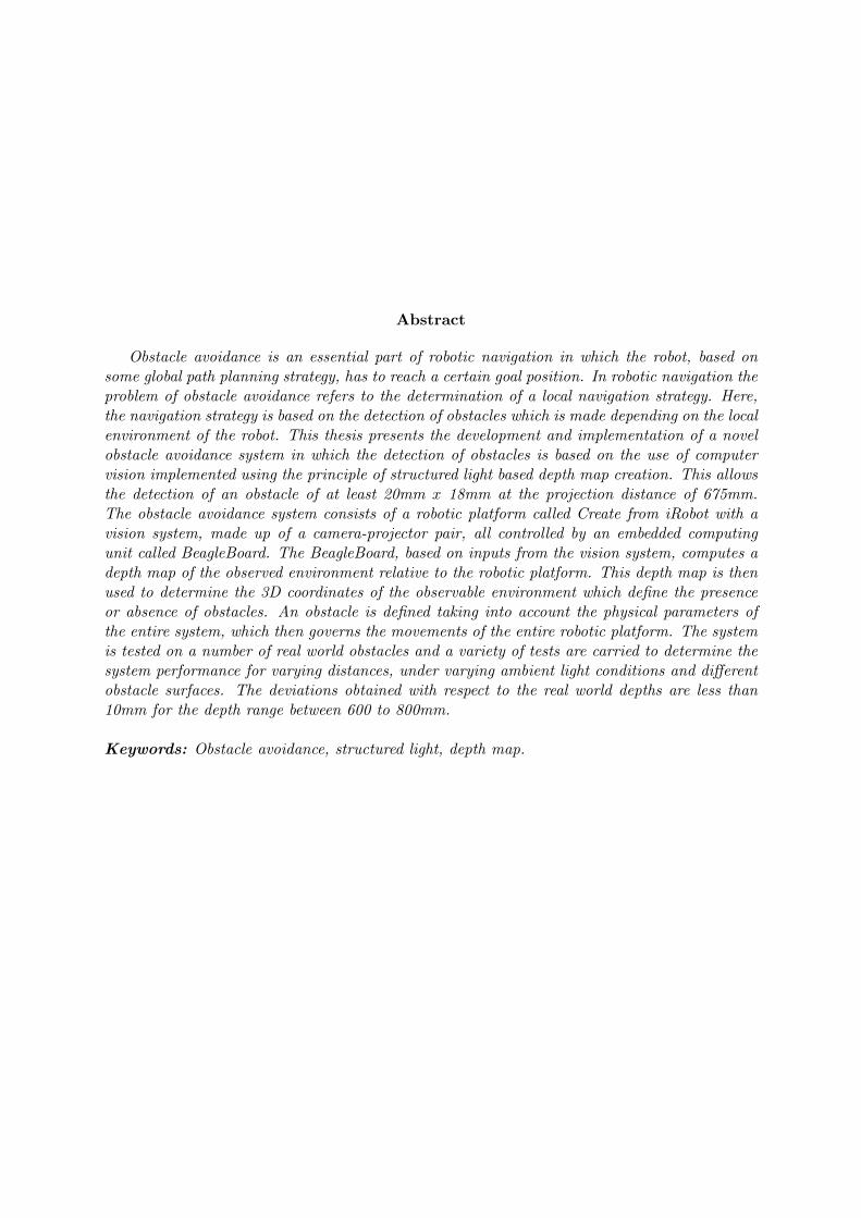
Abstract: Obstacle avoidance is an essential part of robotic navigation in which
the robot, based on some global path planning strategy, has to reach a certain goal position. In robotic navigation the problem of obstacle avoidance refers to the determination of a local navigation strategy. Here, the navigation strategy is based on the detection of obstacles which is made depending on the local environment of the robot. This thesis presents the development and implementation of a novel obstacle avoidance system in which the detection of obstacles is based on the use of computer vision implemented using the principle of structured light based depth map creation. This allows the detection of an obstacle of at least 20mm x 18mm at the projection distance of 675mm. The obstacle avoidance system consists of a robotic platform called Create from iRobot with a vision system, made up of a camera-projector pair, all controlled by an embedded computing unit called BeagleBoard. The BeagleBoard, based on inputs from the vision system, computes a depth map of the observed environment relative to the robotic platform. This depth map is then used to determine the 3D coordinates of the observable environment which define the presence or absence of obstacles. An obstacle is defined taking into account the physical parameters of the entire system, which then governs the movements of the entire robotic platform. The system is tested on a number of real world obstacles and a variety of tests are carried to determine the
system performance for varying distances, under varying ambient light conditions and different obstacle surfaces. The deviations obtained with respect to the real world depths are less than 10mm for the depth range between 600 to 800mm.

PR-TN 2011/00415 Unclassified
iv
Koninklijke Philips Electronics N.V. 2011

Abstract
Obstacle avoidance is an essential part of robotic navigation in which the robot, based onsome global path planning strategy, has to reach a certain goal position. In robotic navigation theproblem of obstacle avoidance refers to the determination of a local navigation strategy. Here,the navigation strategy is based on the detection of obstacles which is made depending on the localenvironment of the robot. This thesis presents the development and implementation of a novelobstacle avoidance system in which the detection of obstacles is based on the use of computervision implemented using the principle of structured light based depth map creation. This allowsthe detection of an obstacle of at least 20mm x 18mm at the projection distance of 675mm.The obstacle avoidance system consists of a robotic platform called Create from iRobot with avision system, made up of a camera-projector pair, all controlled by an embedded computingunit called BeagleBoard. The BeagleBoard, based on inputs from the vision system, computes adepth map of the observed environment relative to the robotic platform. This depth map is thenused to determine the 3D coordinates of the observable environment which define the presenceor absence of obstacles. An obstacle is defined taking into account the physical parameters ofthe entire system, which then governs the movements of the entire robotic platform. The systemis tested on a number of real world obstacles and a variety of tests are carried to determine thesystem performance for varying distances, under varying ambient light conditions and differentobstacle surfaces. The deviations obtained with respect to the real world depths are less than10mm for the depth range between 600 to 800mm.
Keywords: Obstacle avoidance, structured light, depth map.

Dedicated to my parents and my brotherwho have always been a source of inspiration and motivation
in every step of my life.


Acknowledgements
I would firstly like to express my deepest gratitude to my graduation supervisor Prof. Dr.Gerard de Haan for giving me the opportunity to work at Philips Research Eindhoven on thisproject. He has been instrumental in igniting a passion for Video and Image Processing in meand I hope to live up to his expectations in my professional career in the future.
My sincerest thanks to my company supervisor Dr. Frank van Heesch. I feel lucky to havehim as my supervisor, who has never hesitated to find time to listen and help me solve myproblems. He has always encouraged me to be innovative while tackling any problems I facedduring my assignment and I feel a lasting gratitude for all his words of encouragement andsupport. I thank him for having the faith in my abilities to let me work on his project and Ihope I have not disappointed him in any manner. He has not only been a great supervisor butalso a superb friend.
My special thanks to all the researchers at Philips Research Eindhoven and my teachers atthe Eindhoven University of Technology who have always helped me with their timely advicewhenever needed.
I would also like to thank Mr. Sachin Bhardwaj for his review of my thesis and his continuousencouragement and advice during the duration of my graduation project. He has been a greatrole model and a tremendous source of motivation. I thank my friends Ketan Pol, MayurSarode, Mohit Kaushal, Pratik Sahindrakar, Shubhendu Sinha and Vidya Vijayasankaran forall the support, motivation and help they have provided. My special thanks to my best friendHrishikesh who has always provided me with any necessary technical expertise I may havelacked. His words have kept me motivated and smiling and I will always regard him as one ofthe more important reasons for the successes I have achieved.

Contents
1 Introduction 21.1 Problem description . . . . . . . . . . . . . . . . . . . . . . . . . . . . . . . . . . 21.2 Related work . . . . . . . . . . . . . . . . . . . . . . . . . . . . . . . . . . . . . . 31.3 Report Organization . . . . . . . . . . . . . . . . . . . . . . . . . . . . . . . . . . 4
2 Depth estimation 52.1 Depth estimation principle . . . . . . . . . . . . . . . . . . . . . . . . . . . . . . . 5
2.1.1 Human vision . . . . . . . . . . . . . . . . . . . . . . . . . . . . . . . . . . 52.1.2 Correspondence problem . . . . . . . . . . . . . . . . . . . . . . . . . . . . 62.1.3 Stereoscopic machine vision . . . . . . . . . . . . . . . . . . . . . . . . . . 72.1.4 Structured light based depth computation . . . . . . . . . . . . . . . . . . 7
2.1.4.1 Simplified principle . . . . . . . . . . . . . . . . . . . . . . . . . 82.1.4.2 Mathematical analysis . . . . . . . . . . . . . . . . . . . . . . . . 8
2.2 Structured light projection pattern . . . . . . . . . . . . . . . . . . . . . . . . . . 112.2.1 Classification . . . . . . . . . . . . . . . . . . . . . . . . . . . . . . . . . . 11
2.2.1.1 Number of dimensions . . . . . . . . . . . . . . . . . . . . . . . . 112.2.1.2 Multiplexing strategy . . . . . . . . . . . . . . . . . . . . . . . . 122.2.1.3 Coding strategy . . . . . . . . . . . . . . . . . . . . . . . . . . . 132.2.1.4 Pixel depth . . . . . . . . . . . . . . . . . . . . . . . . . . . . . . 14
2.2.2 Finalized pattern . . . . . . . . . . . . . . . . . . . . . . . . . . . . . . . . 142.2.2.1 Pattern encoding . . . . . . . . . . . . . . . . . . . . . . . . . . . 152.2.2.2 Pattern decoding . . . . . . . . . . . . . . . . . . . . . . . . . . . 17
3 System Design 183.1 System setup . . . . . . . . . . . . . . . . . . . . . . . . . . . . . . . . . . . . . . 18
3.1.1 Embedded computing unit . . . . . . . . . . . . . . . . . . . . . . . . . . 193.1.2 Operating System . . . . . . . . . . . . . . . . . . . . . . . . . . . . . . . 193.1.3 Robotic platform . . . . . . . . . . . . . . . . . . . . . . . . . . . . . . . . 193.1.4 Projection system . . . . . . . . . . . . . . . . . . . . . . . . . . . . . . . 20
3.1.4.1 Placement . . . . . . . . . . . . . . . . . . . . . . . . . . . . . . 203.1.4.2 Orientation . . . . . . . . . . . . . . . . . . . . . . . . . . . . . . 213.1.4.3 Projection distance . . . . . . . . . . . . . . . . . . . . . . . . . 21
3.1.5 Camera system . . . . . . . . . . . . . . . . . . . . . . . . . . . . . . . . . 213.1.5.1 Placement . . . . . . . . . . . . . . . . . . . . . . . . . . . . . . 22
3.1.6 Finalized hardware setup . . . . . . . . . . . . . . . . . . . . . . . . . . . 233.2 Calibration . . . . . . . . . . . . . . . . . . . . . . . . . . . . . . . . . . . . . . . 24
iv
3.2.1 System calibration based on Zhang’s method . . . . . . . . . . . . . . . . 243.2.2 Simplified calibration . . . . . . . . . . . . . . . . . . . . . . . . . . . . . 27
3.3 Depth estimation algorithm . . . . . . . . . . . . . . . . . . . . . . . . . . . . . . 293.3.1 Pattern projection . . . . . . . . . . . . . . . . . . . . . . . . . . . . . . . 293.3.2 Image capture . . . . . . . . . . . . . . . . . . . . . . . . . . . . . . . . . 293.3.3 Solution to correspondence problem . . . . . . . . . . . . . . . . . . . . . 29
3.3.3.1 PreProcessing . . . . . . . . . . . . . . . . . . . . . . . . . . . . 303.3.3.2 Grid primitive segmentation . . . . . . . . . . . . . . . . . . . . 313.3.3.3 Grid primitive center location . . . . . . . . . . . . . . . . . . . 313.3.3.4 Grid primitive identification . . . . . . . . . . . . . . . . . . . . 313.3.3.5 4-adjacent neighbors identification . . . . . . . . . . . . . . . . . 333.3.3.6 Projector coordinate computation . . . . . . . . . . . . . . . . . 343.3.3.7 Validity check of computed projector coordinate . . . . . . . . . 35
3.3.4 Depth map computation . . . . . . . . . . . . . . . . . . . . . . . . . . . . 353.3.5 Obstacle detection . . . . . . . . . . . . . . . . . . . . . . . . . . . . . . . 363.3.6 Robotic platform control . . . . . . . . . . . . . . . . . . . . . . . . . . . . 36
4 Results 374.1 Distance tests . . . . . . . . . . . . . . . . . . . . . . . . . . . . . . . . . . . . . . 37
4.1.1 Planar depth . . . . . . . . . . . . . . . . . . . . . . . . . . . . . . . . . . 384.1.2 Multiple planes . . . . . . . . . . . . . . . . . . . . . . . . . . . . . . . . . 384.1.3 Curved surface . . . . . . . . . . . . . . . . . . . . . . . . . . . . . . . . . 394.1.4 Shiny surface . . . . . . . . . . . . . . . . . . . . . . . . . . . . . . . . . . 40
4.2 Ambient light intensity variation . . . . . . . . . . . . . . . . . . . . . . . . . . . 404.3 Effect of depth on measurement accuracy . . . . . . . . . . . . . . . . . . . . . . 414.4 Obstacle detection . . . . . . . . . . . . . . . . . . . . . . . . . . . . . . . . . . . 424.5 Complete system integration . . . . . . . . . . . . . . . . . . . . . . . . . . . . . 434.6 Execution time distribution . . . . . . . . . . . . . . . . . . . . . . . . . . . . . . 44
5 Conclusion and Future Work 45
v
List of Figures
2.1 Disparity in human vision . . . . . . . . . . . . . . . . . . . . . . . . . . . . . . . 62.2 Correspondence problem in stereovision . . . . . . . . . . . . . . . . . . . . . . . 62.3 Depth computation . . . . . . . . . . . . . . . . . . . . . . . . . . . . . . . . . . . 72.4 Hall’s depth computation for coplanar planes . . . . . . . . . . . . . . . . . . . . 82.5 Angles of rotation for non-coplanar planes . . . . . . . . . . . . . . . . . . . . . . 102.6 Coding strategy based on number of dimensions . . . . . . . . . . . . . . . . . . . 112.7 Multiplexing strategies . . . . . . . . . . . . . . . . . . . . . . . . . . . . . . . . . 122.8 Coding strategies . . . . . . . . . . . . . . . . . . . . . . . . . . . . . . . . . . . . 132.9 Coding strategy based on pixel depth . . . . . . . . . . . . . . . . . . . . . . . . 142.10 Projected Pattern . . . . . . . . . . . . . . . . . . . . . . . . . . . . . . . . . . . 162.11 Primitives and spacing . . . . . . . . . . . . . . . . . . . . . . . . . . . . . . . . . 162.12 Decoding window . . . . . . . . . . . . . . . . . . . . . . . . . . . . . . . . . . . . 17
3.1 Project overview . . . . . . . . . . . . . . . . . . . . . . . . . . . . . . . . . . . . 183.2 Create robotic platform . . . . . . . . . . . . . . . . . . . . . . . . . . . . . . . . 193.3 Projector setup . . . . . . . . . . . . . . . . . . . . . . . . . . . . . . . . . . . . . 213.4 Single frame acquisition steps in µEye cameras . . . . . . . . . . . . . . . . . . . 223.5 Final System Setup . . . . . . . . . . . . . . . . . . . . . . . . . . . . . . . . . . . 233.6 Calibration technique based on Zhang’s method . . . . . . . . . . . . . . . . . . . 243.7 Calibration images . . . . . . . . . . . . . . . . . . . . . . . . . . . . . . . . . . . 253.8 Projector - camera orientation . . . . . . . . . . . . . . . . . . . . . . . . . . . . . 263.9 Simplified calibration technique . . . . . . . . . . . . . . . . . . . . . . . . . . . . 273.10 Calibration images placed at different depths . . . . . . . . . . . . . . . . . . . . 283.11 Calibration results . . . . . . . . . . . . . . . . . . . . . . . . . . . . . . . . . . . 283.12 Solving the correspondence problem . . . . . . . . . . . . . . . . . . . . . . . . . 293.13 Binarization . . . . . . . . . . . . . . . . . . . . . . . . . . . . . . . . . . . . . . . 303.14 Filtered output . . . . . . . . . . . . . . . . . . . . . . . . . . . . . . . . . . . . . 303.15 Segmented grid primitives . . . . . . . . . . . . . . . . . . . . . . . . . . . . . . . 313.16 Center location using bounding box . . . . . . . . . . . . . . . . . . . . . . . . . 313.17 Grid primitive location on image plane . . . . . . . . . . . . . . . . . . . . . . . . 323.18 Grid primitive identification using template matching . . . . . . . . . . . . . . . 323.19 Detecting 4-adjacent neighbors . . . . . . . . . . . . . . . . . . . . . . . . . . . . 333.20 Computing the location of grid primitive in structured light pattern . . . . . . . 343.21 Shift of Origin to compute 3D coordinates . . . . . . . . . . . . . . . . . . . . . . 36
4.1 Depth map for planar wall at perpendicular depth of 700mm from system . . . . 384.2 Depth map for perpendicular plane surfaces from system . . . . . . . . . . . . . . 38
vi
4.3 Depth map for curved surface from system . . . . . . . . . . . . . . . . . . . . . . 394.4 Depth map for metallic dustbin . . . . . . . . . . . . . . . . . . . . . . . . . . . . 404.5 Effect of light intensity variation on robustness . . . . . . . . . . . . . . . . . . . 404.6 Error variation with distance . . . . . . . . . . . . . . . . . . . . . . . . . . . . . 414.7 World coordinates for obstacle detection . . . . . . . . . . . . . . . . . . . . . . . 424.8 Platform movement with obstacle . . . . . . . . . . . . . . . . . . . . . . . . . . . 434.9 Relative time consumption for depth computation . . . . . . . . . . . . . . . . . 44
vii

List of Tables
3.1 Intrinsic parameter . . . . . . . . . . . . . . . . . . . . . . . . . . . . . . . . . . . 253.2 Projector extrinsics . . . . . . . . . . . . . . . . . . . . . . . . . . . . . . . . . . . 26
viii

CHAPTER 1
Introduction
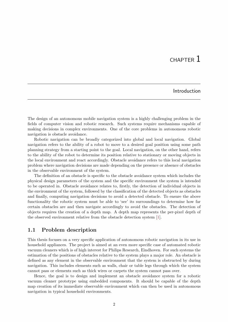
The design of an autonomous mobile navigation system is a highly challenging problem in thefields of computer vision and robotic research. Such systems require mechanisms capable ofmaking decisions in complex environments. One of the core problems in autonomous roboticnavigation is obstacle avoidance.
Robotic navigation can be broadly categorized into global and local navigation. Globalnavigation refers to the ability of a robot to move to a desired goal position using some pathplanning strategy from a starting point to the goal. Local navigation, on the other hand, refersto the ability of the robot to determine its position relative to stationary or moving objects inthe local environment and react accordingly. Obstacle avoidance refers to this local navigationproblem where navigation decisions are made depending on the presence or absence of obstaclesin the observable environment of the system.
The definition of an obstacle is specific to the obstacle avoidance system which includes thephysical design parameters of the system and the specific environment the system is intendedto be operated in. Obstacle avoidance relates to, firstly, the detection of individual objects inthe environment of the system, followed by the classification of the detected objects as obstaclesand finally, computing navigation decisions to avoid a detected obstacle. To ensure the abovefunctionality the robotic system must be able to ‘see’ its surroundings to determine how farcertain obstacles are and then navigate accordingly to avoid the obstacles. The detection ofobjects requires the creation of a depth map. A depth map represents the per-pixel depth ofthe observed environment relative from the obstacle detection system [1].
1.1 Problem description
This thesis focuses on a very specific application of autonomous robotic navigation in its use inhousehold appliances. The project is aimed at an even more specific case of automated roboticvacuum cleaners which is of high interest for Philips Research, Eindhoven. For such systems theestimation of the positions of obstacles relative to the system plays a major role. An obstacle isdefined as any element in the observable environment that the system is obstructed by duringnavigation. This includes elements such as walls, chair or table legs through which the systemcannot pass or elements such as thick wires or carpets the system cannot pass over.
Hence, the goal is to design and implement an obstacle avoidance system for a roboticvacuum cleaner prototype using embedded components. It should be capable of the depthmap creation of its immediate observable environment which can then be used in autonomousnavigation in typical household environments.
2
1.2 Related work
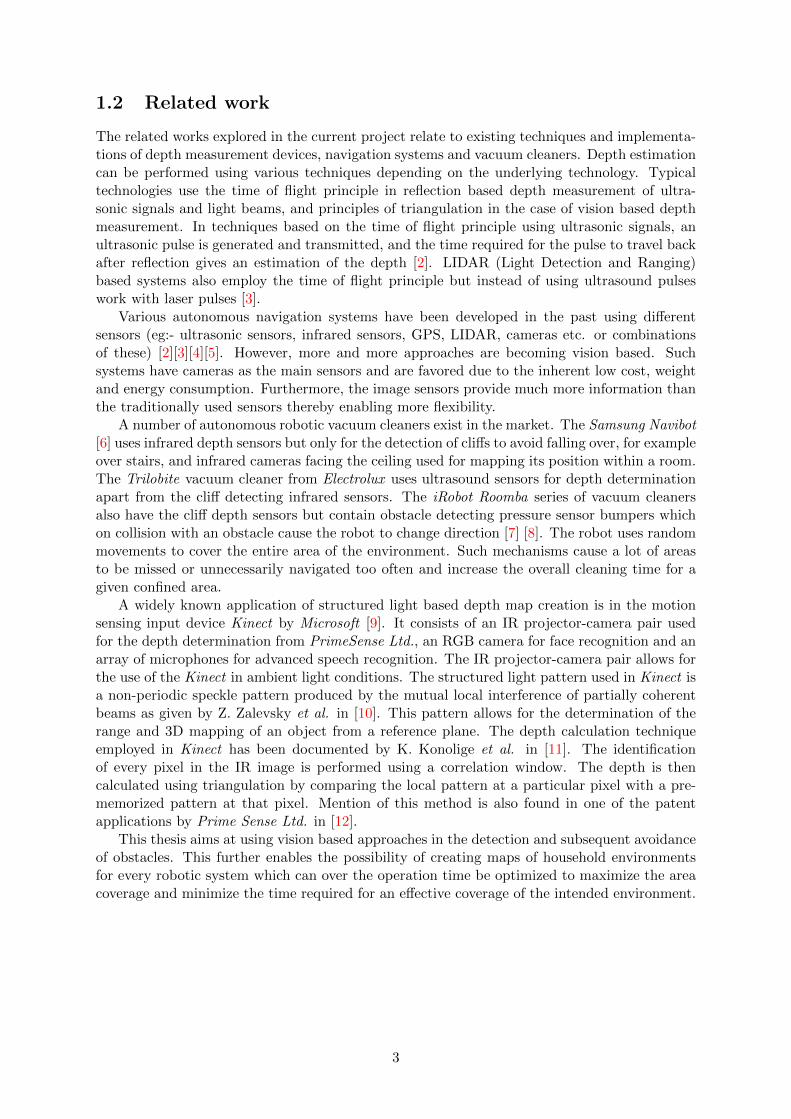
The related works explored in the current project relate to existing techniques and implementa-tions of depth measurement devices, navigation systems and vacuum cleaners. Depth estimationcan be performed using various techniques depending on the underlying technology. Typicaltechnologies use the time of flight principle in reflection based depth measurement of ultra-sonic signals and light beams, and principles of triangulation in the case of vision based depthmeasurement. In techniques based on the time of flight principle using ultrasonic signals, anultrasonic pulse is generated and transmitted, and the time required for the pulse to travel backafter reflection gives an estimation of the depth [2]. LIDAR (Light Detection and Ranging)based systems also employ the time of flight principle but instead of using ultrasound pulseswork with laser pulses [3].
Various autonomous navigation systems have been developed in the past using differentsensors (eg:- ultrasonic sensors, infrared sensors, GPS, LIDAR, cameras etc. or combinationsof these) [2][3][4][5]. However, more and more approaches are becoming vision based. Suchsystems have cameras as the main sensors and are favored due to the inherent low cost, weightand energy consumption. Furthermore, the image sensors provide much more information thanthe traditionally used sensors thereby enabling more flexibility.
A number of autonomous robotic vacuum cleaners exist in the market. The Samsung Navibot[6] uses infrared depth sensors but only for the detection of cliffs to avoid falling over, for exampleover stairs, and infrared cameras facing the ceiling used for mapping its position within a room.The Trilobite vacuum cleaner from Electrolux uses ultrasound sensors for depth determinationapart from the cliff detecting infrared sensors. The iRobot Roomba series of vacuum cleanersalso have the cliff depth sensors but contain obstacle detecting pressure sensor bumpers whichon collision with an obstacle cause the robot to change direction [7] [8]. The robot uses randommovements to cover the entire area of the environment. Such mechanisms cause a lot of areasto be missed or unnecessarily navigated too often and increase the overall cleaning time for agiven confined area.
A widely known application of structured light based depth map creation is in the motionsensing input device Kinect by Microsoft [9]. It consists of an IR projector-camera pair usedfor the depth determination from PrimeSense Ltd., an RGB camera for face recognition and anarray of microphones for advanced speech recognition. The IR projector-camera pair allows forthe use of the Kinect in ambient light conditions. The structured light pattern used in Kinect isa non-periodic speckle pattern produced by the mutual local interference of partially coherentbeams as given by Z. Zalevsky et al. in [10]. This pattern allows for the determination of therange and 3D mapping of an object from a reference plane. The depth calculation techniqueemployed in Kinect has been documented by K. Konolige et al. in [11]. The identificationof every pixel in the IR image is performed using a correlation window. The depth is thencalculated using triangulation by comparing the local pattern at a particular pixel with a pre-memorized pattern at that pixel. Mention of this method is also found in one of the patentapplications by Prime Sense Ltd. in [12].
This thesis aims at using vision based approaches in the detection and subsequent avoidanceof obstacles. This further enables the possibility of creating maps of household environmentsfor every robotic system which can over the operation time be optimized to maximize the areacoverage and minimize the time required for an effective coverage of the intended environment.
3

1.3 Report Organization
This thesis details the various aspects involved in the design and implementation of an auto-mated obstacle avoidance system. Chapter 2 details the principle of depth computation usingcomputer vision. Furthermore, it also contains an overview of the various structured light pat-terns available in literature and ends with the pattern finalized for the current project alongwith its encoding and decoding algorithms. Chapter 3 details the selection criteria for the vari-ous components of the system and the system setup using those components. This chapter alsocontains the calibration methodologies followed, the calibration results obtained and details thealgorithm used for the obstacle avoidance. Chapter 4 gives the results obtained using the systemfor various object surfaces, depths, light conditions and gives the relative time consumption ofthe various parts of the algorithm to solve the correspondence problem. Chapter 5 contains theoverall conclusions and future directions possible for this project.
4
CHAPTER 2
Depth estimation
Depth estimation techniques based on the time of flight principles of ultrasonic or light pulsessuffer from a number of drawbacks. In systems employing such techniques reflections from ob-jects are heavily affected by environmental parameters such as temperature, humidity etc. Theseaffect the velocity of the ultrasonic pulse thereby introducing errors in depth measurement. Fur-thermore, absorptions and refractions of the ultrasound pulse depending on the objects surfaceintroduce additional inaccuracies in depth estimation. Due to the use of the same underlyingprinciple as used in ultrasound based systems, LIDAR also suffers from similar problems. Sys-tems based on time of flight principle require either a number of pulse generator-receiver pairs orcomplex reflection systems to obtain higher spatial resolutions making such systems expensive.
Vision based depth measurement, on the other hand, is less affected by environmental pa-rameters affecting techniques based on the time of flight computation. It refers to the use ofcameras and image processing algorithms for depth measurement. The depth information ispresent due to the disparate views as observed from various camera viewpoints and the depthcan be computed using triangulation techniques. The following sections give detailed descrip-tions of depth estimation principles using vision based technology. In subsequent sections aclassification of special patterns called structured light patterns used for depth measurement isgiven. Finally, the encoding and decoding strategies of a pattern specific to the current projectof obstacle avoidance is described in detail.
2.1 Depth estimation principle
The solution to the problem of vision based depth estimation can be obtained through differentapproaches all related to the triangulation of light rays. Triangulation refers to the computationof depth with the use of geometry and is better explained through examples of human vision.
2.1.1 Human vision
The principle of depth estimation for obstacle avoidance is comparable to the stereopsis principleemployed in e.g. human vision. Stereopsis is the process, in visual perception, that leads to theperception of stereoscopic depth. This is the sensation of depth that emerges from the disparitybetween two different projections of the world on the human retinas.
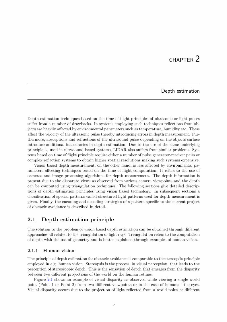
Figure 2.1 shows an example of visual disparity as observed while viewing a single worldpoint (Point 1 or Point 2) from two different viewpoints or in the case of humans - the eyes.Visual disparity occurs due to the projection of light reflected from a world point at different
5
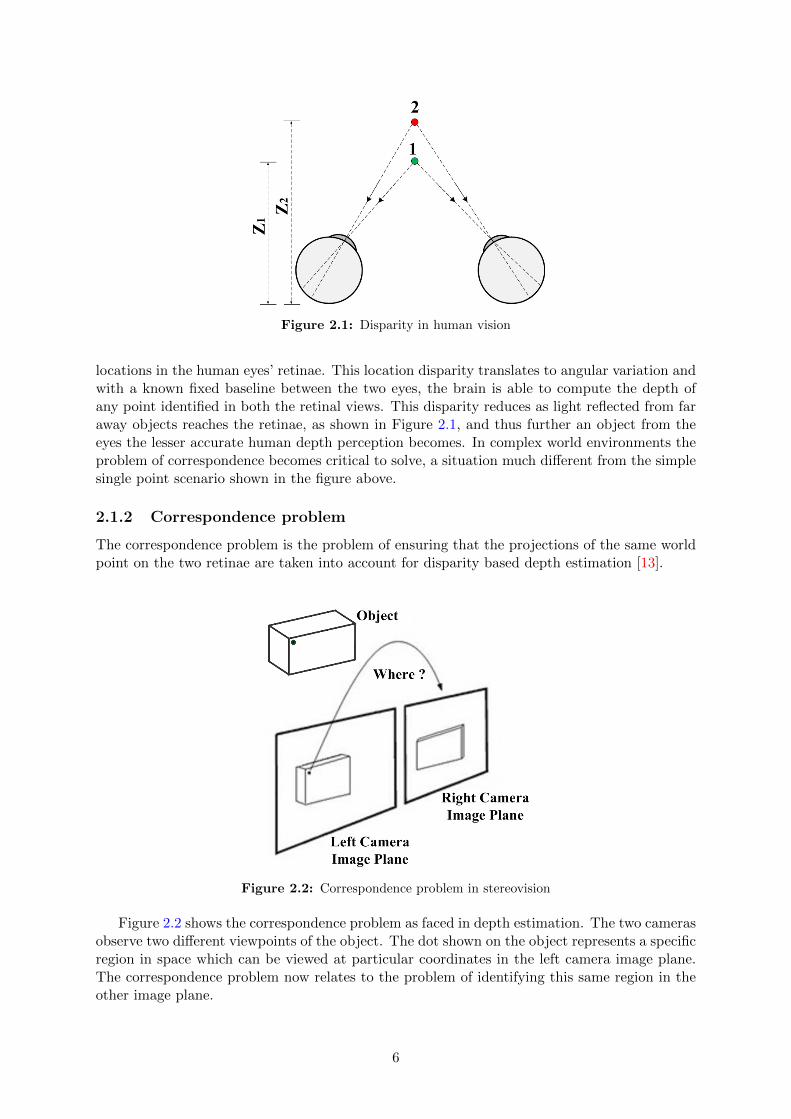
Figure 2.1: Disparity in human vision
locations in the human eyes’ retinae. This location disparity translates to angular variation andwith a known fixed baseline between the two eyes, the brain is able to compute the depth ofany point identified in both the retinal views. This disparity reduces as light reflected from faraway objects reaches the retinae, as shown in Figure 2.1, and thus further an object from theeyes the lesser accurate human depth perception becomes. In complex world environments theproblem of correspondence becomes critical to solve, a situation much different from the simplesingle point scenario shown in the figure above.
2.1.2 Correspondence problem
The correspondence problem is the problem of ensuring that the projections of the same worldpoint on the two retinae are taken into account for disparity based depth estimation [13].
Figure 2.2: Correspondence problem in stereovision
Figure 2.2 shows the correspondence problem as faced in depth estimation. The two camerasobserve two different viewpoints of the object. The dot shown on the object represents a specificregion in space which can be viewed at particular coordinates in the left camera image plane.The correspondence problem now relates to the problem of identifying this same region in theother image plane.
6
2.1.3 Stereoscopic machine vision
The principle of stereopsis can be applied to machine or computer vision with the use of twoor more cameras [14][15][16]. The solution to the correspondence problem is performed usingtechniques such as feature extraction and feature matching between the two or more views. Suchfeatures are typically edges or corners that are searched for within the views. The main drawbackof this method is that such a solution to the correspondence problem is often computationallyexpensive and due to the placements of the cameras or the observable environments, at times,no features might be available for depth map computation. Furthermore, another drawbackof the stereoscopic based systems is the complication increase in low light conditions. Thesystem, thus, inherently requires ambient light for the correct solution to the correspondenceproblem. Even though stereoscopic vision has its drawbacks, in applications with the desiredlight conditions and the presence of appropriate features, depth maps with high resolution andaccuracy can be obtained.
2.1.4 Structured light based depth computation
The use of a structured light based depth computation system highly alleviates the complexityof the correspondence problem. A structured light based system is an active system, obtained byreplacing one of the cameras in a stereoscopic vision system by a projector capable of projectinga desired pattern on the environment to be reconstructed.
Figure 2.3: Depth computation
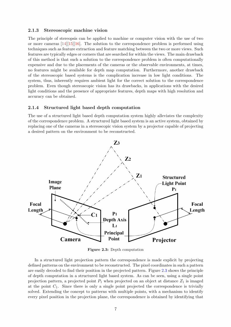
In a structured light projection pattern the correspondence is made explicit by projectingdefined patterns on the environment to be reconstructed. The pixel coordinates in such a patternare easily decoded to find their position in the projected pattern. Figure 2.3 shows the principleof depth computation in a structured light based system. As can be seen, using a single pointprojection pattern, a projected point P1 when projected on an object at distance Z1 is imagedat the point C1. Since there is only a single point projected the correspondence is triviallysolved. Extending the concept to patterns with multiple points, with a mechanism to identifyevery pixel position in the projection plane, the correspondence is obtained by identifying that
7
pixel in the imaging plane. The complexity, robustness, accuracy and resolution of a structurelight based depth computing system depend on the selected structured light pattern. This isanalyzed in depth in Section 2.2.
2.1.4.1 Simplified principle
The simplified principle of depth estimation using structured light can be explained with refer-ence to Figure 2.3. Here, a camera is assumed to be simplified to a pinhole model and a projectorto be originating from a point source (an inverse pinhole-camera model). The projection andcamera planes are at a distance focal length in front of their respective focus points. A struc-tured light pattern point P1 projected at a distance Z1, is imaged at the ray-plane intersectionpoint on the camera plane. For varying depths of a particular projection point (Z1, Z2, Z3),the imaged point is always found to lie on a line L1 in the camera plane. With the knowledgeof the L1, the location of an imaged point on the line directly corresponds to the depth. Here,depth is defined as the perpendicular distance of the world point from a fixed point in the depthcomputation system. To simultaneously compute the depth of multiple points in an observablescene a structured light pattern with multiple points can be used.
2.1.4.2 Mathematical analysis
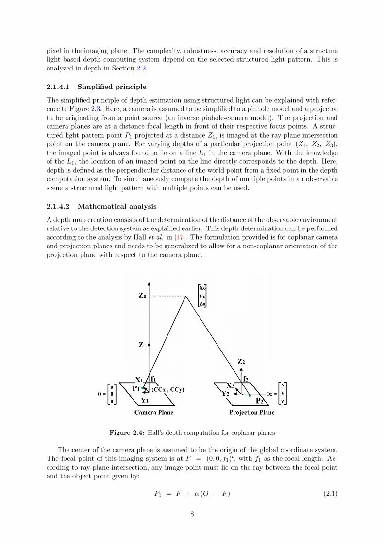
A depth map creation consists of the determination of the distance of the observable environmentrelative to the detection system as explained earlier. This depth determination can be performedaccording to the analysis by Hall et al. in [17]. The formulation provided is for coplanar cameraand projection planes and needs to be generalized to allow for a non-coplanar orientation of theprojection plane with respect to the camera plane.
Figure 2.4: Hall’s depth computation for coplanar planes
The center of the camera plane is assumed to be the origin of the global coordinate system.The focal point of this imaging system is at F = (0, 0, f1)
t, with f1 as the focal length. Ac-cording to ray-plane intersection, any image point must lie on the ray between the focal pointand the object point given by:
P1 = F + α (O − F ) (2.1)
8
Here, P1 represents the coordinates of the object point on the image plane with respect to theglobal origin - the center of the camera plane.Equation 2.1 is expanded as: xi
yi0
=
00f1
+ α
xoyo
zo − f1
(2.2)
where, O = (xo, yo, zo)t represents the object point and
α =f1
f1 − zo(2.3)
From equations 2.2 and 2.1 the object coordinates can be computed as:
xo =
(f1 − zof1
)xi and yo =
(f1 − zof1
)yi (2.4)
Equation 2.4 can be modified assuming a virtual image plane in front of the focal point. Thisallows the direct use of image plane coordinates to compute the height and width dimensionsfrom the depth value with the knowledge of the intrinsic parameters of the camera. xi and yiare the image coordinates and to compute the world coordinates need to be converted takinginto account its relative position to the principal point of the camera (CCx, CCy), the pixelpitch and the direction of x and y axes. For the orientation as shown in Figure 2.4 the objectcoordinates with respect to the global origin as the camera center are given as:
xo(mm) =
(zo − 2 ∗ f1
f1
)∗ (CCx − xi) ∗ PixelP itch
yo(mm) =
(zo − 2 ∗ f1
f1
)∗ (CCy − yi) ∗ PixelP itch (2.5)
Assuming O2 = (x2, y2, z2)t represents the center of the projection plane with respect to
the global origin, F2 = (0, 0, f2)t represents the focal point of the projection plane with respect
to the local origin or F2 = (x2, y2, z2 +f2)t with respect to the global origin, and the projected
point corresponding to the imaged point P1 is represented as P2 = (x2 +x2i, y2 + y2i, z2)t with
respect to the global origin. The coordinate (x2i, y2i, 0)t represents the point corresponding tothe imaged point P1 with respect to the origin of the projection system.
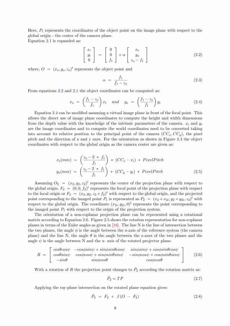
The orientation of a non-coplanar projection plane can be represented using a rotationalmatrix according to Equation 2.6. Figure 2.5 shows the rotation representation for non-coplanarplanes in terms of the Euler angles as given in [18]. The line N is the line of intersection betweenthe two planes, the angle φ is the angle between the x-axis of the reference system (the cameraplane) and the line N, the angle θ is the angle between the z-axes of the two planes and theangle ψ is the angle between N and the x- axis of the rotated projector plane.
R =
cosθcosψ −cosφsinψ + sinφsinθcosψ sinφsinψ + cosφsinθcosψcosθsinψ cosφcosψ + sinφsinθsinψ −sinφcosψ + cosφsinθsinψ−sinθ sinφcosθ cosφcosθ
(2.6)
With a rotation of R the projection point changes to P̂2 according the rotation matrix as:
P̂2 = TP (2.7)
Applying the ray-plane intersection on the rotated plane equation gives:
P̂2 = F2 + β (O − F2) (2.8)
9
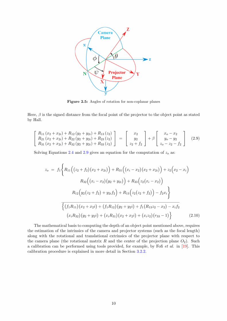
Figure 2.5: Angles of rotation for non-coplanar planes
Here, β is the signed distance from the focal point of the projector to the object point as statedby Hall.
R11 (x2 + x2i) +R12 (y2 + y2i) +R13 (z2)R21 (x2 + x2i) +R22 (y2 + y2i) +R23 (z2)R31 (x2 + x2i) +R32 (y2 + y2i) +R33 (z2)
=
x2y2
z2 + f2
+ β
xo − x2yo − y2
zo − z2 − f2
(2.9)
Solving Equations 2.4 and 2.9 gives an equation for the computation of zo as:
zo = f1
{R11
((z2 + f2
)(x2 + x2i
))+R31
((xi − x2
)(x2 + x2i
))+ z2
(x2 − xi
)R32
((xi − x2
)(y2 + y2i
))+R33
(z2(xi − x2
))R12
(y2(z2 + f2
)+ y2if2
)+R13
(z2(z2 + f2
))− f2xi
}{(f1R11
)(x2 + x2i
)+(f1R12
)(y2 + y2i
)+ f1
(R13z2 − x2
)− xif2(
xiR32
)(y2 + y2i
)+(xiR31
)(x2 + x2i
)+(xiz2
)(r33 − 1
)}(2.10)
The mathematical basis to computing the depth of an object point mentioned above, requiresthe estimation of the intrinsics of the camera and projector systems (such as the focal length)along with the rotational and translational extrinsics of the projector plane with respect tothe camera plane (the rotational matrix R and the center of the projection plane O2). Sucha calibration can be performed using tools provided, for example, by Fofi et al. in [19]. Thiscalibration procedure is explained in more detail in Section 3.2.2.
10
2.2 Structured light projection pattern
In this section the various structured light patterns available in the literature are surveyed andfinally a pattern suitable for the current application is designed.
2.2.1 Classification
The design of structured light patterns has evolved over the years after a large amount of researchdone in this field of computer vision. The projected pattern is designed with the intention ofuniquely identifying each pixel in the projection pattern, done by either coding the pixel with itsrow or column position information or both. Structured light patterns are classified accordingto various pattern design parameters. Classifications are based upon the number of dimensionsthe pattern has, the multiplexing strategy used, the coding strategy used and the pixel depthof the patterns. Such classifications are explained in more detail in the sections below:
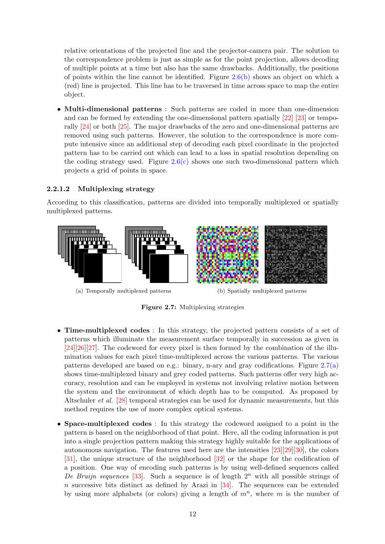
2.2.1.1 Number of dimensions
Structured light patterns can be classified according to the number of dimensions the pattern ismade up of. These can be zero-dimensional points, a one-dimensional line or multi-dimensionalpatterns.
(a) Zero-dimensional point (b) One-Dimensional line (c) Multi-dimensional pattern
Figure 2.6: Coding strategy based on number of dimensions
• Zero-dimensional points : A pattern consisting of a single point is the simplest form ofa structured light pattern. The location of the projected point from the projection planeis known and the single point captured on the image plane can easily be identified. Thisensures a simple and fast solution to the correspondence problem for a single point. How-ever, such systems suffer from some major drawbacks. Firstly, for such point projectionsthe depth of only a single point in space can be computed at a time instant, thus thesingle point pattern has to be extended in space and time by moving the point projectionacross the environment to be mapped. Such an extension increases the time required toscan any given area, reducing the efficiency of the entire system. Secondly, systems em-ploying such projection strategies cannot be used in applications requiring relative motionbetween the system and the region to be mapped, since at one time instant only a singlepoint can be mapped. Finally, a separate system needs to be implemented so as to movethe single projection point across the scene to be mapped. This if done at a very high ratecan completely remove the earlier drawbacks. Figure 2.6(a) shows an example of such apattern with the red dot indicating the point projected at a given time instant and thearrows showing the area traversing direction.
• One-dimensional lines : Improving on the point based structured light systems, a singleline can be projected [20] [21]. A major constraint here is that the projected line mustbe perpendicular to the displacement between the projector-camera pair. This allows thesolution to the correspondence problem for an entire row or column depending on the
11
relative orientations of the projected line and the projector-camera pair. The solution tothe correspondence problem is just as simple as for the point projection, allows decodingof multiple points at a time but also has the same drawbacks. Additionally, the positionsof points within the line cannot be identified. Figure 2.6(b) shows an object on which a(red) line is projected. This line has to be traversed in time across space to map the entireobject.
• Multi-dimensional patterns : Such patterns are coded in more than one-dimensionand can be formed by extending the one-dimensional pattern spatially [22] [23] or tempo-rally [24] or both [25]. The major drawbacks of the zero and one-dimensional patterns areremoved using such patterns. However, the solution to the correspondence is more com-pute intensive since an additional step of decoding each pixel coordinate in the projectedpattern has to be carried out which can lead to a loss in spatial resolution depending onthe coding strategy used. Figure 2.6(c) shows one such two-dimensional pattern whichprojects a grid of points in space.
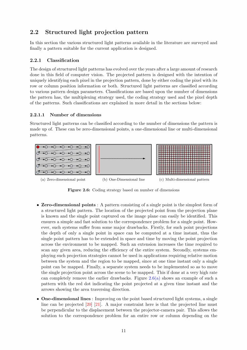
2.2.1.2 Multiplexing strategy
According to this classification, patterns are divided into temporally multiplexed or spatiallymultiplexed patterns.
(a) Temporally multiplexed patterns (b) Spatially multiplexed patterns
Figure 2.7: Multiplexing strategies
• Time-multiplexed codes : In this strategy, the projected pattern consists of a set ofpatterns which illuminate the measurement surface temporally in succession as given in[24][26][27]. The codeword for every pixel is then formed by the combination of the illu-mination values for each pixel time-multiplexed across the various patterns. The variouspatterns developed are based on e.g.: binary, n-ary and gray codifications. Figure 2.7(a)shows time-multiplexed binary and grey coded patterns. Such patterns offer very high ac-curacy, resolution and can be employed in systems not involving relative motion betweenthe system and the environment of which depth has to be computed. As proposed byAltschuler et al. [28] temporal strategies can be used for dynamic measurements, but thismethod requires the use of more complex optical systems.
• Space-multiplexed codes : In this strategy the codeword assigned to a point in thepattern is based on the neighborhood of that point. Here, all the coding information is putinto a single projection pattern making this strategy highly suitable for the applications ofautonomous navigation. The features used here are the intensities [23][29][30], the colors[31], the unique structure of the neighborhood [32] or the shape for the codification ofa position. One way of encoding such patterns is by using well-defined sequences calledDe Bruijn sequences [33]. Such a sequence is of length 2n with all possible strings ofn successive bits distinct as defined by Arazi in [34]. The sequences can be extendedby using more alphabets (or colors) giving a length of mn, where m is the number of
12
alphabets used. Figure 2.7(b) shows examples of spatially multiplexed patterns. Suchpatterns necessitate the identification of the sub-blocks of pixels which have the specialcolor or spatial property associated with them.
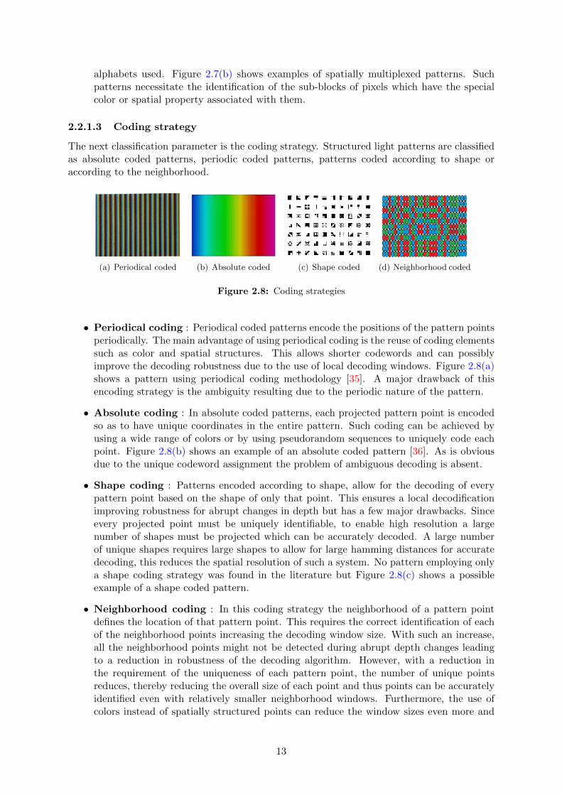
2.2.1.3 Coding strategy
The next classification parameter is the coding strategy. Structured light patterns are classifiedas absolute coded patterns, periodic coded patterns, patterns coded according to shape oraccording to the neighborhood.
(a) Periodical coded (b) Absolute coded (c) Shape coded (d) Neighborhood coded
Figure 2.8: Coding strategies
• Periodical coding : Periodical coded patterns encode the positions of the pattern pointsperiodically. The main advantage of using periodical coding is the reuse of coding elementssuch as color and spatial structures. This allows shorter codewords and can possiblyimprove the decoding robustness due to the use of local decoding windows. Figure 2.8(a)shows a pattern using periodical coding methodology [35]. A major drawback of thisencoding strategy is the ambiguity resulting due to the periodic nature of the pattern.
• Absolute coding : In absolute coded patterns, each projected pattern point is encodedso as to have unique coordinates in the entire pattern. Such coding can be achieved byusing a wide range of colors or by using pseudorandom sequences to uniquely code eachpoint. Figure 2.8(b) shows an example of an absolute coded pattern [36]. As is obviousdue to the unique codeword assignment the problem of ambiguous decoding is absent.
• Shape coding : Patterns encoded according to shape, allow for the decoding of everypattern point based on the shape of only that point. This ensures a local decodificationimproving robustness for abrupt changes in depth but has a few major drawbacks. Sinceevery projected point must be uniquely identifiable, to enable high resolution a largenumber of shapes must be projected which can be accurately decoded. A large numberof unique shapes requires large shapes to allow for large hamming distances for accuratedecoding, this reduces the spatial resolution of such a system. No pattern employing onlya shape coding strategy was found in the literature but Figure 2.8(c) shows a possibleexample of a shape coded pattern.
• Neighborhood coding : In this coding strategy the neighborhood of a pattern pointdefines the location of that pattern point. This requires the correct identification of eachof the neighborhood points increasing the decoding window size. With such an increase,all the neighborhood points might not be detected during abrupt depth changes leadingto a reduction in robustness of the decoding algorithm. However, with a reduction inthe requirement of the uniqueness of each pattern point, the number of unique pointsreduces, thereby reducing the overall size of each point and thus points can be accuratelyidentified even with relatively smaller neighborhood windows. Furthermore, the use ofcolors instead of spatially structured points can reduce the window sizes even more and
13
leads to patterns with higher spatial resolutions. Such neighborhoods can be formed intime or in space. Figure 2.8(d) shows one such pattern as given in [37].
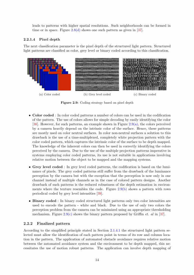
2.2.1.4 Pixel depth
The next classification parameter is the pixel depth of the structured light pattern. Structuredlight patterns are classified as color, grey level or binary coded according to this classification.
(a) Color coded (b) Grey level coded (c) Binary coded
Figure 2.9: Coding strategy based on pixel depth
• Color coded : In color coded patterns a number of colors can be used in the codificationof the pattern. The use of colors allows for simple decoding by easily identifying the color[38]. However, for such patterns, an example shown in Figure 2.9(a), the colors perceivedby a camera heavily depend on the intrinsic color of the surface. Hence, these patternsare mostly used on color neutral surfaces. In color non-neutral surfaces a solution to thisdrawback is the use of a time-multiplexed, completely white projection pattern with thecolor coded pattern, which captures the intrinsic color of the surface to be depth mapped.The knowledge of the inherent colors can then be used in correctly identifying the colorsperceived by the camera. Due to the use of the multiple projection patterns imperative insystems employing color coded patterns, its use is not suitable in applications involvingrelative motion between the object to be mapped and the mapping systems.
• Grey level coded : In grey level coded patterns, the codification is based on the lumi-nance of pixels. The grey coded patterns still suffer from the drawback of the luminanceperception by the camera but with the exception that the perception is now only in onechannel instead of multiple channels as in the case of colored pattern designs. Anotherdrawback of such patterns is the reduced robustness of the depth estimation in environ-ments where the texture resembles the code. Figure 2.9(b) shows a pattern with rowsperiodical coded by grey level intensities [39].
• Binary coded : In binary coded structured light patterns only two color intensities areused to encode the pattern - white and black. Due to the use of only two colors theperception problem from the camera can be minimized using an appropriate thresholdingmechanism. Figure 2.9(c) shows the binary pattern proposed by Griffin et. al in [37].
2.2.2 Finalized pattern
According to the simplified principle stated in Section 2.1.4.1 the structured light pattern se-lected must allow the identification of each pattern point in terms of its row and column loca-tion in the pattern. The application of automated obstacle avoidance requires relative motionbetween the automated avoidance system and the environment to be depth mapped, this ne-cessitates the use of motion robust patterns. The application can involve depth mapping of
14
surfaces with a lot of discontinuities, which makes it imperative to use patterns with smalldecoding windows. Finally, the use-case scenarios of color non-neutral environments providesanother constraint in the selection of the structured light pattern.
With the above constraints in mind the pattern chosen, suggested by Griffin et al. in [37],is two-dimensional and spatially multiplexed to be motion robust. It also has to be absolute-neighborhood coded with a small neighborhood to allow for unique identification of all patternpoints and minimizing surface discontinuity errors. Finally, the pattern must be binary in pixeldepth to work in color non-neutral environments. Additionally, as stated by Griffin, the patternmust consist of unique spatially designed grid primitives instead of color coded primitives tocope for the color non-neutral environments. The next sections detail the encoding and decodingmethodology of the selected pattern.
2.2.2.1 Pattern encoding
The encoding methodology of the pattern requires the formation of a (M,N) 2D De BruijnSequence (dBS), where M is the number of columns and N the rows. This requires the formationof a (P, 3) and (P, 2) dBS and then using those two sequences to form the 2D dBS. A (i, j) dBSis a sequence of length ij , with characters ∈ [1, P ], where every possible subsequence of length jappears as a continuous sequence of characters exactly once. The pattern is generated accordingto the following steps:
1. Selection of P : The span of the dBS (P ) is selected depending on the spatial resolutionrequirements of the application. For the current application the entire structured lightpattern should be at least equal to the working area of the robotic platform. Selecting thepattern dimension exactly equal to the working area at a given projection distance givesthe most efficient use of the available camera resolution and allows for the detection ofobstacles in the platform’s path. The computation of the working area is given in detail inChapter 3. A span of P = 4 gives a spatial resolution adequate for the current application.
2. Formation of (i, j) De Bruijn Sequence : The generation of a (i, j) dBS is as given byHsieh in [40]. Following the procedure results in an efficient decoding methodology andyields the (P, 3) and (P, 2) dBS respectively as:
G(P,3) = 4443442441433432431423422421413412411333233132232131231122212111G(P,2) = 4434241332312211
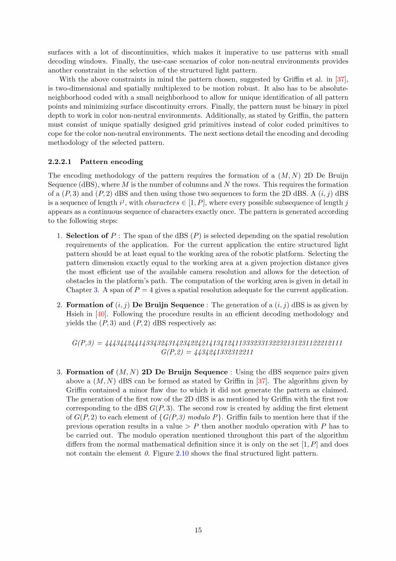
3. Formation of (M,N) 2D De Bruijn Sequence : Using the dBS sequence pairs givenabove a (M,N) dBS can be formed as stated by Griffin in [37]. The algorithm given byGriffin contained a minor flaw due to which it did not generate the pattern as claimed.The generation of the first row of the 2D dBS is as mentioned by Griffin with the first rowcorresponding to the dBS G(P, 3). The second row is created by adding the first elementof G(P, 2) to each element of {G(P,3) modulo P}. Griffin fails to mention here that if theprevious operation results in a value > P then another modulo operation with P has tobe carried out. The modulo operation mentioned throughout this part of the algorithmdiffers from the normal mathematical definition since it is only on the set [1, P ] and doesnot contain the element 0. Figure 2.10 shows the final structured light pattern.
15
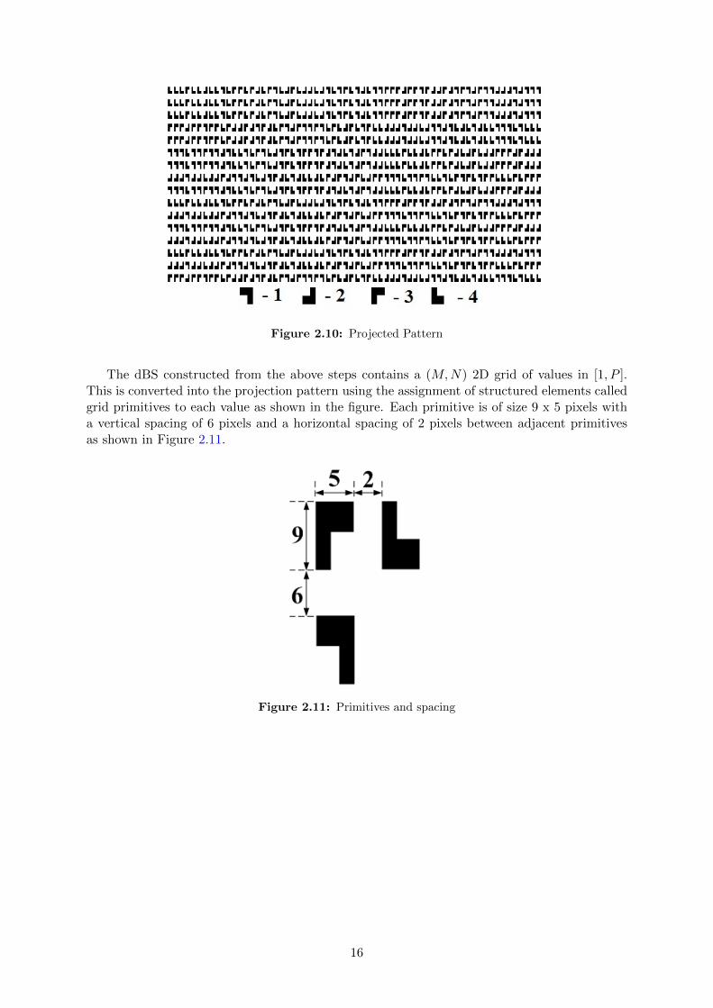
Figure 2.10: Projected Pattern
The dBS constructed from the above steps contains a (M,N) 2D grid of values in [1, P ].This is converted into the projection pattern using the assignment of structured elements calledgrid primitives to each value as shown in the figure. Each primitive is of size 9 x 5 pixels witha vertical spacing of 6 pixels and a horizontal spacing of 2 pixels between adjacent primitivesas shown in Figure 2.11.
Figure 2.11: Primitives and spacing
16
2.2.2.2 Pattern decoding
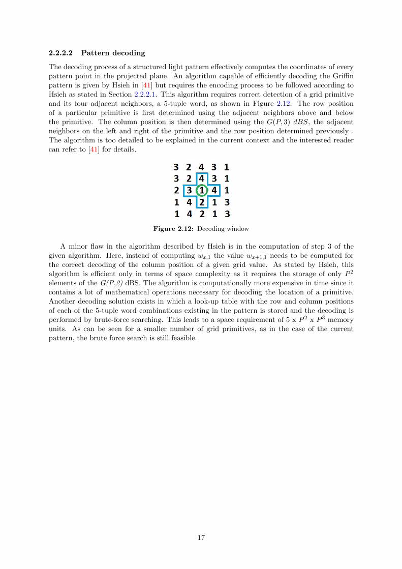
The decoding process of a structured light pattern effectively computes the coordinates of everypattern point in the projected plane. An algorithm capable of efficiently decoding the Griffinpattern is given by Hsieh in [41] but requires the encoding process to be followed according toHsieh as stated in Section 2.2.2.1. This algorithm requires correct detection of a grid primitiveand its four adjacent neighbors, a 5-tuple word, as shown in Figure 2.12. The row positionof a particular primitive is first determined using the adjacent neighbors above and belowthe primitive. The column position is then determined using the G(P, 3) dBS, the adjacentneighbors on the left and right of the primitive and the row position determined previously .The algorithm is too detailed to be explained in the current context and the interested readercan refer to [41] for details.
Figure 2.12: Decoding window
A minor flaw in the algorithm described by Hsieh is in the computation of step 3 of thegiven algorithm. Here, instead of computing wx,1 the value wx+1,1 needs to be computed forthe correct decoding of the column position of a given grid value. As stated by Hsieh, thisalgorithm is efficient only in terms of space complexity as it requires the storage of only P 2
elements of the G(P,2) dBS. The algorithm is computationally more expensive in time since itcontains a lot of mathematical operations necessary for decoding the location of a primitive.Another decoding solution exists in which a look-up table with the row and column positionsof each of the 5-tuple word combinations existing in the pattern is stored and the decoding isperformed by brute-force searching. This leads to a space requirement of 5 x P 2 x P 3 memoryunits. As can be seen for a smaller number of grid primitives, as in the case of the currentpattern, the brute force search is still feasible.
17
CHAPTER 3
System Design
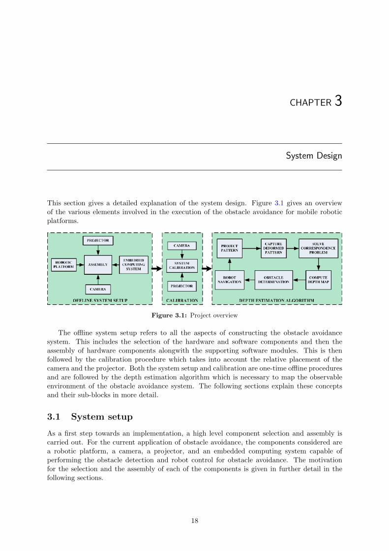
This section gives a detailed explanation of the system design. Figure 3.1 gives an overviewof the various elements involved in the execution of the obstacle avoidance for mobile roboticplatforms.
Figure 3.1: Project overview
The offline system setup refers to all the aspects of constructing the obstacle avoidancesystem. This includes the selection of the hardware and software components and then theassembly of hardware components alongwith the supporting software modules. This is thenfollowed by the calibration procedure which takes into account the relative placement of thecamera and the projector. Both the system setup and calibration are one-time offline proceduresand are followed by the depth estimation algorithm which is necessary to map the observableenvironment of the obstacle avoidance system. The following sections explain these conceptsand their sub-blocks in more detail.
3.1 System setup
As a first step towards an implementation, a high level component selection and assembly iscarried out. For the current application of obstacle avoidance, the components considered area robotic platform, a camera, a projector, and an embedded computing system capable ofperforming the obstacle detection and robot control for obstacle avoidance. The motivationfor the selection and the assembly of each of the components is given in further detail in thefollowing sections.
18
3.1.1 Embedded computing unit
The embedded computing unit is the heart of the navigation system controlling the entiresystem. It needs to be able to communicate with and control the camera, the projector andthe robotic platform to efficiently achieve the goal of automated navigation. One system thatsatisfies all these constraints is the BeagleBoard by Texas Instruments [42]. It contains an ARMcore as the CPU, with additional peripheral connections for USB, RS-232 communication andDVI-D.
3.1.2 Operating System
The selection of an appropriate operating system (OS) is one of the main aspects which affectsthe development of the obstacle avoidance system employing the BeagleBoard. The main factorsin the selection of the OS were economic aspects such as cost and licensing charges and theavailability of drives necessary for the interface with the various elements of the system. Theopen source Linux based Angstrom distribution [43] was found to be the ideal OS for theBeagleBoard for the current application, since it was the only freely available OS having driversfor the interface with the selected camera system. This requirement is mentioned in depth inSection 3.1.5. For an easier development with the BeagleBoard system supplementary softwarepackages need to be used. Packages for the I2C communication over DVI-D, compilers andlibraries for the development of software etc. not supplied with the operating system had to beadditionally installed.
3.1.3 Robotic platform
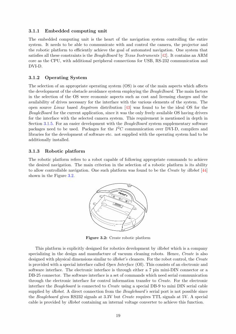
The robotic platform refers to a robot capable of following appropriate commands to achievethe desired navigation. The main criterion in the selection of a robotic platform is its abilityto allow controllable navigation. One such platform was found to be the Create by iRobot [44]shown in the Figure 3.2.
Figure 3.2: Create robotic platform
This platform is explicitly designed for robotics development by iRobot which is a companyspecializing in the design and manufacture of vacuum cleaning robots. Hence, Create is alsodesigned with physical dimensions similar to iRobot’s cleaners. For the robot control, the Createis provided with a special interface called Open Interface (OI). This consists of an electronic andsoftware interface. The electronic interface is through either a 7 pin mini-DIN connector or aDB-25 connector. The software interface is a set of commands which need serial communicationthrough the electronic interface for control information transfer to Create. For the electronicinterface the Beagleboard is connected to Create using a special DB-9 to mini DIN serial cablesupplied by iRobot. A direct connection from the Beagleboard’s serial port is not possible sincethe Beagleboard gives RS232 signals at 3.3V but Create requires TTL signals at 5V. A specialcable is provided by iRobot containing an internal voltage converter to achieve this function.
19
The commands for the control of Create to be used in the current project are mentionedbelow:
• Before sending any command to Create a Start command has to be sent which starts theOI.
Command: [128].
• The drive command controls Create’s drive wheels. This requires two other parametersto be given - the velocity and the radius. Velocity is a value in the range -500 to 500mm/s and radius between -2000 to 2000mm. The radius is measured from the centerof the turning circle to the center of Create. A drive command with a positive velocityand positive radius makes Create drive forward while turning left, while a negative radiusmakes it turn right. Both these parameters are represented in 16-bit 2’s compliment.
Command: [137][Velocity high byte][Velocity low byte][Radius highbyte][Radius low byte]
• Special cases of drive commands are:
– Straight = [8000] or [7FFF] in hex
– Turn in place clockwise = [FFFF] in hex
– Turn in place counter-clockwise = [0001] in hex
• Create contains an internal mechanism which determines how much distance it has traveledwhich can be used in defining the range of movement of the platform. This distance isdefined in mm and also needs to be represented in 16-bit 2’s compliment.
Command: [156][Distance high byte][Distance low byte]
3.1.4 Projection system
The projection system must be capable of projecting the selected projection pattern which is thefirst step in the solution of the correspondence problem. The Pico projector system developedby Texas Instruments [45] allows for an easy construction of a desired projection pattern andhas a very small form factor motivating its selection as the projection system. This projectorsupports a suitable resolution of 320 x 480 and connects to the BeagleBoard using the HDMIconnection with the control being handled by the Angstrom OS through I2C communication.The placement of the projector, with respect to its placement on the platform and its orientation,forms a very important part of the system setup as it determines the depth computation areaof the entire system.
3.1.4.1 Placement
The projector has to be placed on the top of the robotic platform due to the design of theplatform. To ensure minimum angular distortion on the projected plane the projector should beas close to the central line of the robotic platform as possible. A wide gap between the projectorand this central line results in a deformed projection as shown in Figure 3.3(c). Due to thestructure of the projector heat sink the minimum off-center displacement for the projector’scenter is 30mm.
20
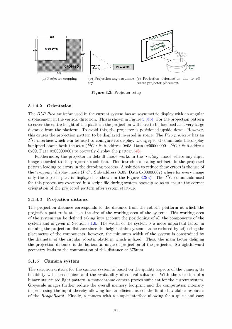
(a) Projector cropping (b) Projection angle asymme-try
(c) Projection deformation due to off-center projector placement
Figure 3.3: Projector setup
3.1.4.2 Orientation
The DLP Pico projector used in the current system has an asymmetric display with an angulardisplacement in the vertical direction. This is shown in Figure 3.3(b). For the projection patternto cover the entire height of the platform the projection will have to be focussed at a very largedistance from the platform. To avoid this, the projector is positioned upside down. However,this causes the projection pattern to be displayed inverted in space. The Pico projector has anI2C interface which can be used to configure its display. Using special commands the displayis flipped about both the axes (I2C : Sub-address 0x08, Data 0x00000000 ; I2C : Sub-address0x09, Data 0x00000000) to correctly display the pattern [46].
Furthermore, the projector in default mode works in the ‘scaling ’ mode where any inputimage is scaled to the projector resolution. This introduces scaling artifacts in the projectedpattern leading to errors in the decoding process. A solution to reduce these errors is the use ofthe ‘cropping ’ display mode (I2C : Sub-address 0x05, Data 0x00000007) where for every imageonly the top-left part is displayed as shown in the Figure 3.3(a). The I2C commands usedfor this process are executed in a script file during system boot-up so as to ensure the correctorientation of the projected pattern after system start-up.
3.1.4.3 Projection distance
The projection distance corresponds to the distance from the robotic platform at which theprojection pattern is at least the size of the working area of the system. This working areaof the system can be defined taking into account the positioning of all the components of thesystem and is given in Section 3.1.6. The width of the system is a more important factor indefining the projection distance since the height of the system can be reduced by adjusting theplacements of the components, however, the minimum width of the system is constrained bythe diameter of the circular robotic platform which is fixed. Thus, the main factor definingthe projection distance is the horizontal angle of projection of the projector. Straightforwardgeometry leads to the computation of this distance at 675mm.
3.1.5 Camera system
The selection criteria for the camera system is based on the quality aspects of the camera, itsflexibility with lens choices and the availability of control software. With the selection of abinary structured light pattern, a monochrome camera proves sufficient for the current system.Greyscale images further reduce the overall memory footprint and the computation intensityin processing the input thereby allowing for an efficient use of the limited available resourcesof the BeagleBoard. Finally, a camera with a simple interface allowing for a quick and easy
21

development is preferred. The µEyeUI122xLE −M USB camera by iDS, with the additionaladvantage of allowing varifocal S-mount lenses, was chosen since it satisfied all the previousconstraints. It also allowed for more flexibility with control over a number of internal featuressuch as resolution, frame rate, region of interest etc.
Figure 3.4: Single frame acquisition steps in µEye cameras
The camera was a major selection criterion in the finalization of the OS for the BeagleBoardsince its drivers were not developed for use on every OS and processor architecture combination.The drivers provided by iDS allowed for extremely slow single frame acquisitions at approx. 1fps, which would not prove adequate for a robot navigation system and were only available asbinaries preventing modifications to allow for more control. Using the APIs provided, a newcontrol software was developed, according to the steps in Figure 3.4. As a first step the cameraneeds to be initialized with parameters for exposure time and the pixel depth. In the next step,memory is allocated and set for the frame to be captured. The frame capture is carried outnext using an appropriate software trigger and the captured frame is saved to memory. Thisframe is then used in the computation of the 3D coordinates as explained in Section 3.3. Itwas found that the bottleneck in achieving the desired frame rate was the initialization step ofthe frame acquisition. By using a single initialization followed by sequential frame acquisitionsthe frame rate could be improved to 10 fps. This, however, made it mandatory for the depthestimation to be performed sequentially after the frame acquisition. For higher frame rates thevideo mode feature of the cameras could be used.
3.1.5.1 Placement
Similar to the placement of the projection system the camera also has to be placed on topof the robotic platform. To allow for focussing at the projection distance and to cover theworking area by the image plane, a S-mount varifocal lens is used. The camera is placed asclose to the central line of the robotic platform as possible so as to reduce distortions causeddue to the angular imaging. However, this allows for smaller displacements in the imagedprojected pattern for varying depths. Increasing the distance between the camera-projector pairincreases the disparity leading to higher accuracy in the depth measurement but increases theocclusions caused due to an increased angular separation between the optical axes. An increasein occlusions reduces the spatial area which can be depth mapped, lowering the resolution ofthe entire system.
22
3.1.6 Finalized hardware setup
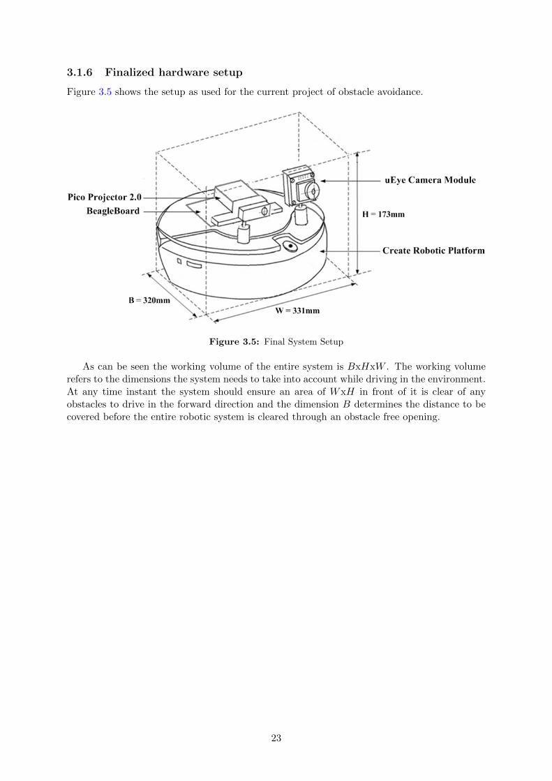
Figure 3.5 shows the setup as used for the current project of obstacle avoidance.
Figure 3.5: Final System Setup
As can be seen the working volume of the entire system is BxHxW . The working volumerefers to the dimensions the system needs to take into account while driving in the environment.At any time instant the system should ensure an area of WxH in front of it is clear of anyobstacles to drive in the forward direction and the dimension B determines the distance to becovered before the entire robotic system is cleared through an obstacle free opening.
23
3.2 Calibration
System calibration is a necessary step in the computation of 3D coordinates. In this thesis, twocalibration procedures were implemented. The first procedure is based on Zhang’s calibrationmethod [47] and aims to be used to determine the intrinsic and extrinsic parameters necessaryfor the depth estimation according to the mathematical analysis, while the second one is asimplified procedure developed to efficiently compute the depth. Both the calibration proceduresare explained in further detail in the following sections.
3.2.1 System calibration based on Zhang’s method
In this calibration procedure intrinsic and extrinsic parameters for the camera, the projectorand the visual system as a whole are computed. This is in accordance to the mathematicalanalysis presented in Section 2.1.4.2, which states that a calibration procedure must precededepth estimation.
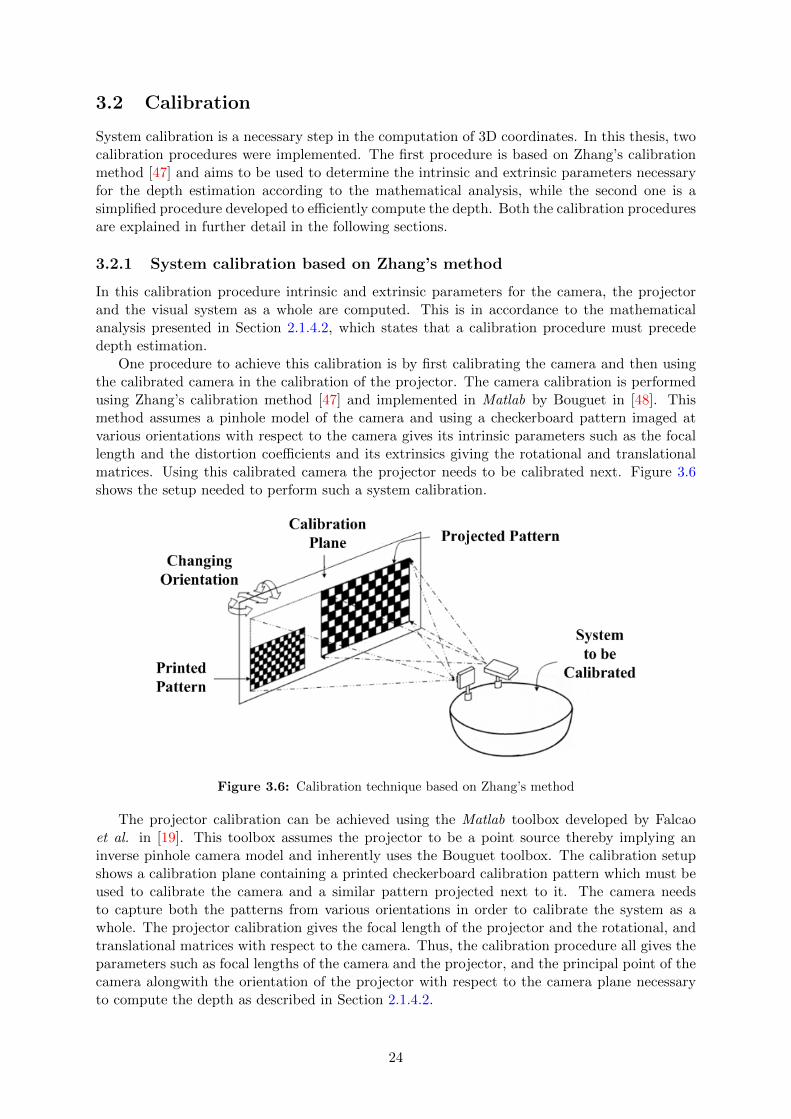
One procedure to achieve this calibration is by first calibrating the camera and then usingthe calibrated camera in the calibration of the projector. The camera calibration is performedusing Zhang’s calibration method [47] and implemented in Matlab by Bouguet in [48]. Thismethod assumes a pinhole model of the camera and using a checkerboard pattern imaged atvarious orientations with respect to the camera gives its intrinsic parameters such as the focallength and the distortion coefficients and its extrinsics giving the rotational and translationalmatrices. Using this calibrated camera the projector needs to be calibrated next. Figure 3.6shows the setup needed to perform such a system calibration.
Figure 3.6: Calibration technique based on Zhang’s method
The projector calibration can be achieved using the Matlab toolbox developed by Falcaoet al. in [19]. This toolbox assumes the projector to be a point source thereby implying aninverse pinhole camera model and inherently uses the Bouguet toolbox. The calibration setupshows a calibration plane containing a printed checkerboard calibration pattern which must beused to calibrate the camera and a similar pattern projected next to it. The camera needsto capture both the patterns from various orientations in order to calibrate the system as awhole. The projector calibration gives the focal length of the projector and the rotational, andtranslational matrices with respect to the camera. Thus, the calibration procedure all gives theparameters such as focal lengths of the camera and the projector, and the principal point of thecamera alongwith the orientation of the projector with respect to the camera plane necessaryto compute the depth as described in Section 2.1.4.2.
24
Calibration results
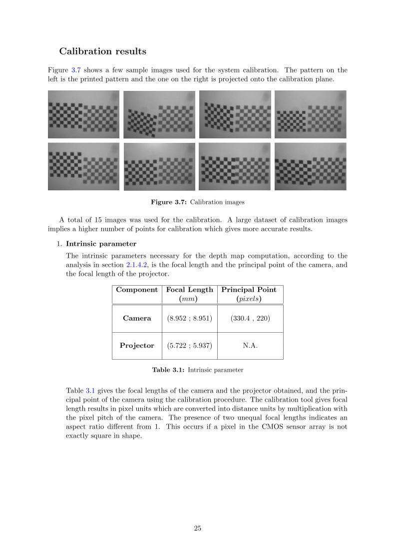
Figure 3.7 shows a few sample images used for the system calibration. The pattern on theleft is the printed pattern and the one on the right is projected onto the calibration plane.
Figure 3.7: Calibration images
A total of 15 images was used for the calibration. A large dataset of calibration imagesimplies a higher number of points for calibration which gives more accurate results.
1. Intrinsic parameter
The intrinsic parameters necessary for the depth map computation, according to theanalysis in section 2.1.4.2, is the focal length and the principal point of the camera, andthe focal length of the projector.
Component Focal Length Principal Point(mm) (pixels)
Camera (8.952 ; 8.951) (330.4 , 220)
Projector (5.722 ; 5.937) N.A.
Table 3.1: Intrinsic parameter
Table 3.1 gives the focal lengths of the camera and the projector obtained, and the prin-cipal point of the camera using the calibration procedure. The calibration tool gives focallength results in pixel units which are converted into distance units by multiplication withthe pixel pitch of the camera. The presence of two unequal focal lengths indicates anaspect ratio different from 1. This occurs if a pixel in the CMOS sensor array is notexactly square in shape.
25
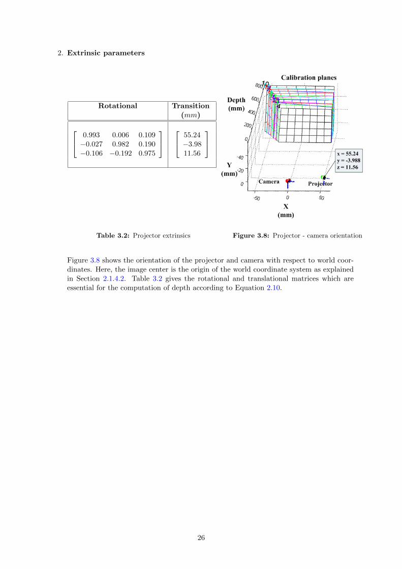
2. Extrinsic parameters
Rotational Transition(mm)
0.993 0.006 0.109−0.027 0.982 0.190−0.106 −0.192 0.975
55.24−3.9811.56
Table 3.2: Projector extrinsics Figure 3.8: Projector - camera orientation
Figure 3.8 shows the orientation of the projector and camera with respect to world coor-dinates. Here, the image center is the origin of the world coordinate system as explainedin Section 2.1.4.2. Table 3.2 gives the rotational and translational matrices which areessential for the computation of depth according to Equation 2.10.
26
3.2.2 Simplified calibration
Since the above mentioned calibration methods provide extremely accurate models for camera-projector pair systems not necessary for the current application of obstacle detection, a simplercalibration method is implemented which exploits the basic principle of depth estimation asgiven in Section 2.1.4.1. This calibration allows for a simple and, hence, a fast depth computa-tion once the correspondence problem has been solved.
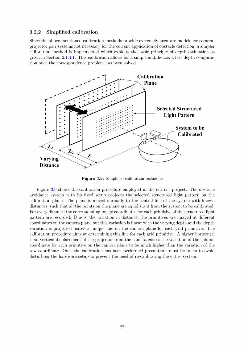
Figure 3.9: Simplified calibration technique
Figure 3.9 shows the calibration procedure employed in the current project. The obstacleavoidance system with its fixed setup projects the selected structured light pattern on thecalibration plane. The plane is moved normally to the central line of the system with knowndistances, such that all the points on the plane are equidistant from the system to be calibrated.For every distance the corresponding image coordinates for each primitive of the structured lightpattern are recorded. Due to the variation in distance, the primitives are imaged at differentcoordinates on the camera plane but this variation is linear with the varying depth and the depthvariation is projected across a unique line on the camera plane for each grid primitive. Thecalibration procedure aims at determining this line for each grid primitive. A higher horizontalthan vertical displacement of the projector from the camera causes the variation of the columncoordinate for each primitive on the camera plane to be much higher than the variation of therow coordinate. Once the calibration has been performed precautions must be taken to avoiddisturbing the hardware setup to prevent the need of re-calibrating the entire system.
27
Calibration results
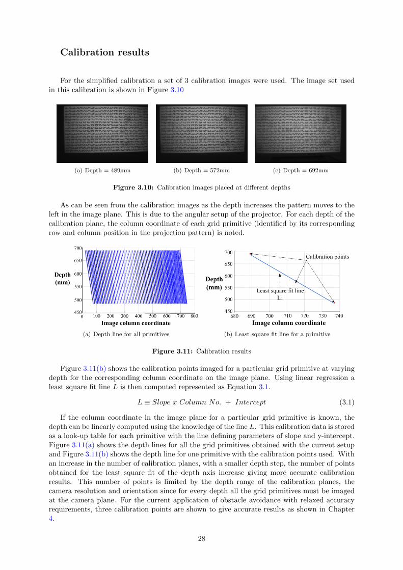
For the simplified calibration a set of 3 calibration images were used. The image set usedin this calibration is shown in Figure 3.10
(a) Depth = 489mm (b) Depth = 572mm (c) Depth = 692mm
Figure 3.10: Calibration images placed at different depths
As can be seen from the calibration images as the depth increases the pattern moves to theleft in the image plane. This is due to the angular setup of the projector. For each depth of thecalibration plane, the column coordinate of each grid primitive (identified by its correspondingrow and column position in the projection pattern) is noted.
(a) Depth line for all primitives (b) Least square fit line for a primitive
Figure 3.11: Calibration results
Figure 3.11(b) shows the calibration points imaged for a particular grid primitive at varyingdepth for the corresponding column coordinate on the image plane. Using linear regression aleast square fit line L is then computed represented as Equation 3.1.
L ≡ Slope x Column No. + Intercept (3.1)
If the column coordinate in the image plane for a particular grid primitive is known, thedepth can be linearly computed using the knowledge of the line L. This calibration data is storedas a look-up table for each primitive with the line defining parameters of slope and y-intercept.Figure 3.11(a) shows the depth lines for all the grid primitives obtained with the current setupand Figure 3.11(b) shows the depth line for one primitive with the calibration points used. Withan increase in the number of calibration planes, with a smaller depth step, the number of pointsobtained for the least square fit of the depth axis increase giving more accurate calibrationresults. This number of points is limited by the depth range of the calibration planes, thecamera resolution and orientation since for every depth all the grid primitives must be imagedat the camera plane. For the current application of obstacle avoidance with relaxed accuracyrequirements, three calibration points are shown to give accurate results as shown in Chapter4.
28
3.3 Depth estimation algorithm
With the system setup and the calibration performed, the system can be deployed in desiredenvironments to estimate depths. In this section a detailed description of the algorithm used toachieve this goal is given. The algorithm follows the sequence of operations as given in Figure3.1. Each of the steps of the algorithm are explained in detail in the sections below.
3.3.1 Pattern projection
The first step in the depth determination algorithm is the projection of the structured lightpattern. Since a single frame pattern is selected for the current application of obstacle avoidance,a simple image viewer (e.g. GQView) can be used to achieve projection using the selected Picoprojector.
3.3.2 Image capture
The projected pattern deforms due to the depth variations in the observable environment to bemapped. This is captured using the µEye camera selected.
3.3.3 Solution to correspondence problem
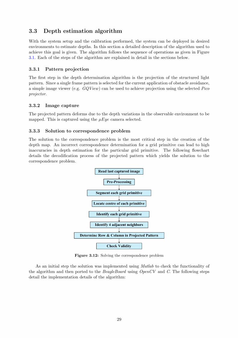
The solution to the correspondence problem is the most critical step in the creation of thedepth map. An incorrect correspondence determination for a grid primitive can lead to highinaccuracies in depth estimation for the particular grid primitive. The following flowchartdetails the decodification process of the projected pattern which yields the solution to thecorrespondence problem.
Figure 3.12: Solving the correspondence problem
As an initial step the solution was implemented using Matlab to check the functionality ofthe algorithm and then ported to the BeagleBoard using OpenCV and C. The following stepsdetail the implementation details of the algorithm:
29
3.3.3.1 PreProcessing
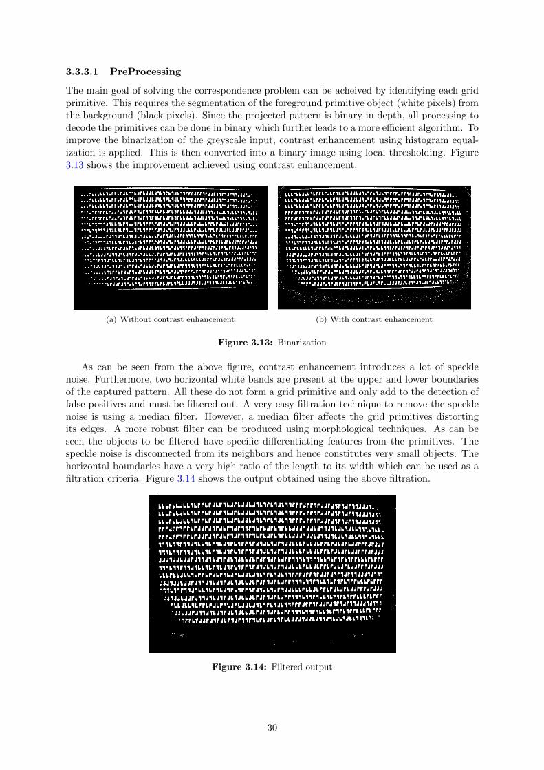
The main goal of solving the correspondence problem can be acheived by identifying each gridprimitive. This requires the segmentation of the foreground primitive object (white pixels) fromthe background (black pixels). Since the projected pattern is binary in depth, all processing todecode the primitives can be done in binary which further leads to a more efficient algorithm. Toimprove the binarization of the greyscale input, contrast enhancement using histogram equal-ization is applied. This is then converted into a binary image using local thresholding. Figure3.13 shows the improvement achieved using contrast enhancement.
(a) Without contrast enhancement (b) With contrast enhancement
Figure 3.13: Binarization
As can be seen from the above figure, contrast enhancement introduces a lot of specklenoise. Furthermore, two horizontal white bands are present at the upper and lower boundariesof the captured pattern. All these do not form a grid primitive and only add to the detection offalse positives and must be filtered out. A very easy filtration technique to remove the specklenoise is using a median filter. However, a median filter affects the grid primitives distortingits edges. A more robust filter can be produced using morphological techniques. As can beseen the objects to be filtered have specific differentiating features from the primitives. Thespeckle noise is disconnected from its neighbors and hence constitutes very small objects. Thehorizontal boundaries have a very high ratio of the length to its width which can be used as afiltration criteria. Figure 3.14 shows the output obtained using the above filtration.
Figure 3.14: Filtered output
30
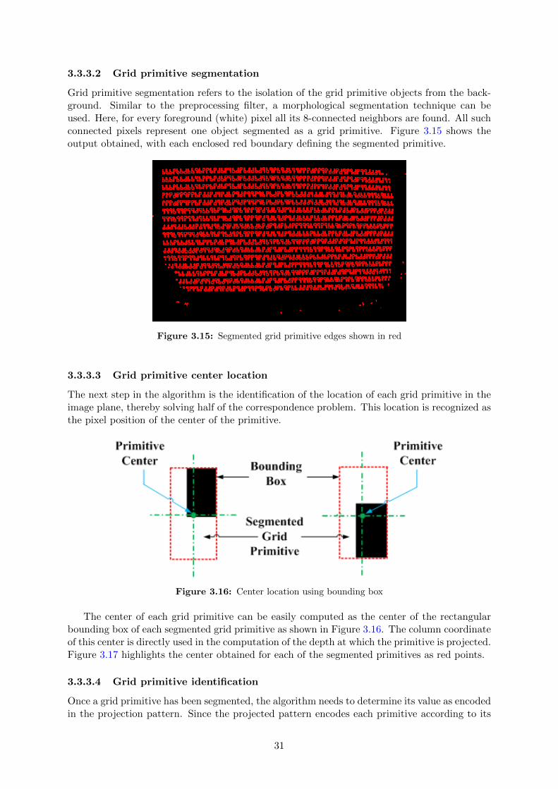
3.3.3.2 Grid primitive segmentation
Grid primitive segmentation refers to the isolation of the grid primitive objects from the back-ground. Similar to the preprocessing filter, a morphological segmentation technique can beused. Here, for every foreground (white) pixel all its 8-connected neighbors are found. All suchconnected pixels represent one object segmented as a grid primitive. Figure 3.15 shows theoutput obtained, with each enclosed red boundary defining the segmented primitive.
Figure 3.15: Segmented grid primitive edges shown in red
3.3.3.3 Grid primitive center location
The next step in the algorithm is the identification of the location of each grid primitive in theimage plane, thereby solving half of the correspondence problem. This location is recognized asthe pixel position of the center of the primitive.
Figure 3.16: Center location using bounding box
The center of each grid primitive can be easily computed as the center of the rectangularbounding box of each segmented grid primitive as shown in Figure 3.16. The column coordinateof this center is directly used in the computation of the depth at which the primitive is projected.Figure 3.17 highlights the center obtained for each of the segmented primitives as red points.
3.3.3.4 Grid primitive identification
Once a grid primitive has been segmented, the algorithm needs to determine its value as encodedin the projection pattern. Since the projected pattern encodes each primitive according to its
31
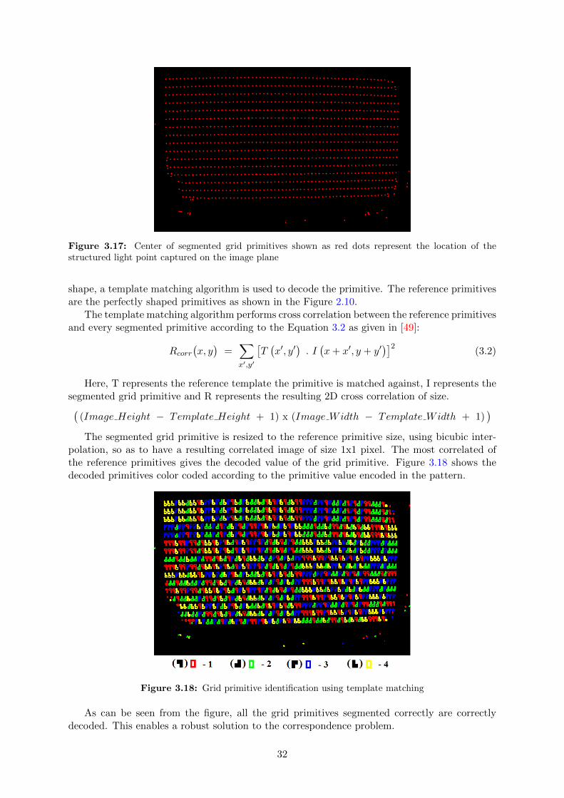
Figure 3.17: Center of segmented grid primitives shown as red dots represent the location of thestructured light point captured on the image plane
shape, a template matching algorithm is used to decode the primitive. The reference primitivesare the perfectly shaped primitives as shown in the Figure 2.10.
The template matching algorithm performs cross correlation between the reference primitivesand every segmented primitive according to the Equation 3.2 as given in [49]:
Rcorr
(x, y)
=∑x′,y′
[T(x′, y′
). I(x+ x′, y + y′
)]2(3.2)
Here, T represents the reference template the primitive is matched against, I represents thesegmented grid primitive and R represents the resulting 2D cross correlation of size.(
(Image Height − Template Height + 1) x (Image Width − Template Width + 1))
The segmented grid primitive is resized to the reference primitive size, using bicubic inter-polation, so as to have a resulting correlated image of size 1x1 pixel. The most correlated ofthe reference primitives gives the decoded value of the grid primitive. Figure 3.18 shows thedecoded primitives color coded according to the primitive value encoded in the pattern.
Figure 3.18: Grid primitive identification using template matching
As can be seen from the figure, all the grid primitives segmented correctly are correctlydecoded. This enables a robust solution to the correspondence problem.
32
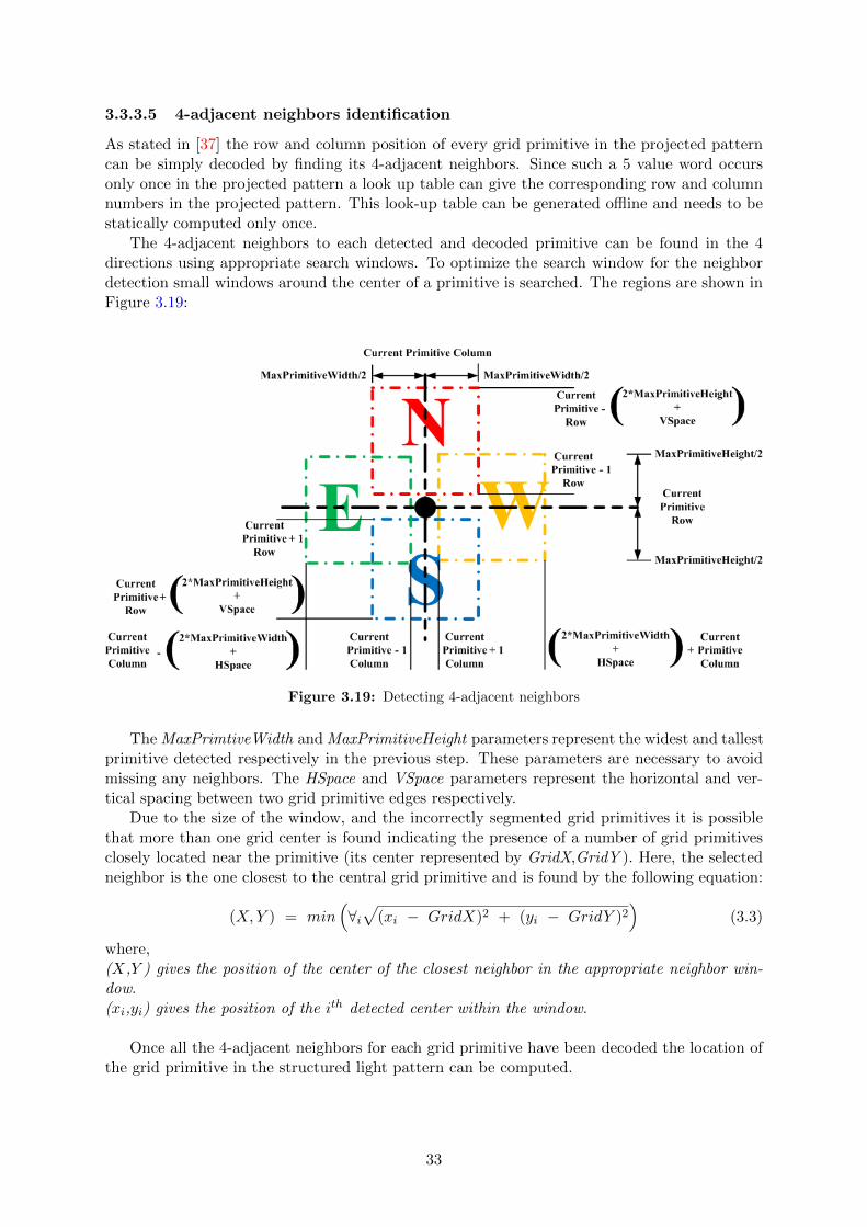
3.3.3.5 4-adjacent neighbors identification
As stated in [37] the row and column position of every grid primitive in the projected patterncan be simply decoded by finding its 4-adjacent neighbors. Since such a 5 value word occursonly once in the projected pattern a look up table can give the corresponding row and columnnumbers in the projected pattern. This look-up table can be generated offline and needs to bestatically computed only once.
The 4-adjacent neighbors to each detected and decoded primitive can be found in the 4directions using appropriate search windows. To optimize the search window for the neighbordetection small windows around the center of a primitive is searched. The regions are shown inFigure 3.19:
Figure 3.19: Detecting 4-adjacent neighbors
The MaxPrimtiveWidth and MaxPrimitiveHeight parameters represent the widest and tallestprimitive detected respectively in the previous step. These parameters are necessary to avoidmissing any neighbors. The HSpace and VSpace parameters represent the horizontal and ver-tical spacing between two grid primitive edges respectively.
Due to the size of the window, and the incorrectly segmented grid primitives it is possiblethat more than one grid center is found indicating the presence of a number of grid primitivesclosely located near the primitive (its center represented by GridX,GridY ). Here, the selectedneighbor is the one closest to the central grid primitive and is found by the following equation:
(X,Y ) = min(∀i√
(xi − GridX)2 + (yi − GridY )2)
(3.3)
where,(X,Y ) gives the position of the center of the closest neighbor in the appropriate neighbor win-dow.(xi,yi) gives the position of the ith detected center within the window.
Once all the 4-adjacent neighbors for each grid primitive have been decoded the location ofthe grid primitive in the structured light pattern can be computed.
33
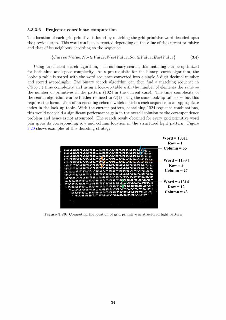
3.3.3.6 Projector coordinate computation
The location of each grid primitive is found by matching the grid primitive word decoded uptothe previous step. This word can be constructed depending on the value of the current primitiveand that of its neighbors according to the sequence:
{CurrentV alue,NorthV alue,WestV alue, SouthV alue,EastV alue} (3.4)
Using an efficient search algorithm, such as binary search, this matching can be optimizedfor both time and space complexity. As a pre-requisite for the binary search algorithm, thelook-up table is sorted with the word sequence converted into a single 5 digit decimal numberand stored accordingly. The binary search algorithm can then find a matching sequence inO(log n) time complexity and using a look-up table with the number of elements the same asthe number of primitives in the pattern (1024 in the current case). The time complexity ofthe search algorithm can be further reduced to O(1) using the same look-up table size but thisrequires the formulation of an encoding scheme which matches each sequence to an appropriateindex in the look-up table. With the current pattern, containing 1024 sequence combinations,this would not yield a significant performance gain in the overall solution to the correspondenceproblem and hence is not attempted. The search result obtained for every grid primitive wordpair gives its corresponding row and column location in the structured light pattern. Figure3.20 shows examples of this decoding strategy.
Figure 3.20: Computing the location of grid primitive in structured light pattern
34
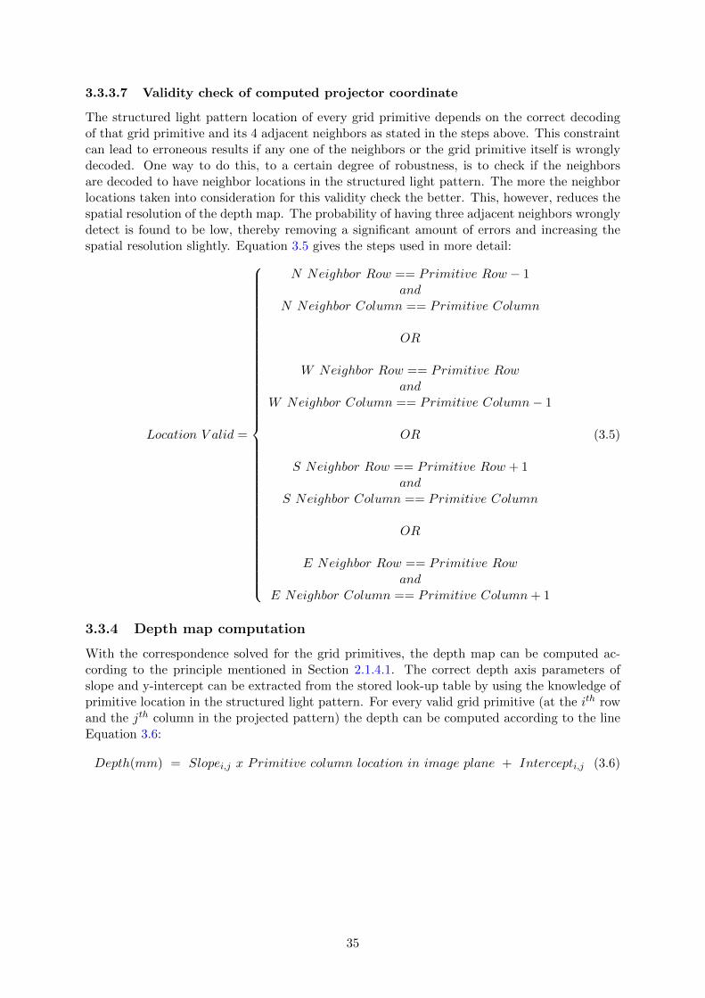
3.3.3.7 Validity check of computed projector coordinate
The structured light pattern location of every grid primitive depends on the correct decodingof that grid primitive and its 4 adjacent neighbors as stated in the steps above. This constraintcan lead to erroneous results if any one of the neighbors or the grid primitive itself is wronglydecoded. One way to do this, to a certain degree of robustness, is to check if the neighborsare decoded to have neighbor locations in the structured light pattern. The more the neighborlocations taken into consideration for this validity check the better. This, however, reduces thespatial resolution of the depth map. The probability of having three adjacent neighbors wronglydetect is found to be low, thereby removing a significant amount of errors and increasing thespatial resolution slightly. Equation 3.5 gives the steps used in more detail:
Location V alid =
N Neighbor Row == Primitive Row − 1and
N Neighbor Column == Primitive Column
OR
W Neighbor Row == Primitive Rowand
W Neighbor Column == Primitive Column− 1
OR
S Neighbor Row == Primitive Row + 1and
S Neighbor Column == Primitive Column
OR
E Neighbor Row == Primitive Rowand
E Neighbor Column == Primitive Column+ 1
(3.5)
3.3.4 Depth map computation
With the correspondence solved for the grid primitives, the depth map can be computed ac-cording to the principle mentioned in Section 2.1.4.1. The correct depth axis parameters ofslope and y-intercept can be extracted from the stored look-up table by using the knowledge ofprimitive location in the structured light pattern. For every valid grid primitive (at the ith rowand the jth column in the projected pattern) the depth can be computed according to the lineEquation 3.6:
Depth(mm) = Slopei,j x Primitive column location in image plane + Intercepti,j (3.6)
35
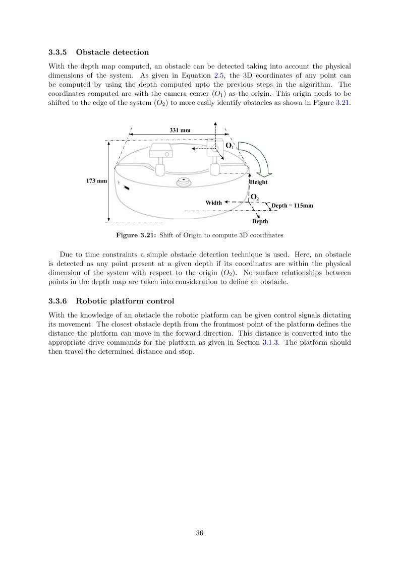
3.3.5 Obstacle detection
With the depth map computed, an obstacle can be detected taking into account the physicaldimensions of the system. As given in Equation 2.5, the 3D coordinates of any point canbe computed by using the depth computed upto the previous steps in the algorithm. Thecoordinates computed are with the camera center (O1) as the origin. This origin needs to beshifted to the edge of the system (O2) to more easily identify obstacles as shown in Figure 3.21.
Figure 3.21: Shift of Origin to compute 3D coordinates
Due to time constraints a simple obstacle detection technique is used. Here, an obstacleis detected as any point present at a given depth if its coordinates are within the physicaldimension of the system with respect to the origin (O2). No surface relationships betweenpoints in the depth map are taken into consideration to define an obstacle.
3.3.6 Robotic platform control
With the knowledge of an obstacle the robotic platform can be given control signals dictatingits movement. The closest obstacle depth from the frontmost point of the platform defines thedistance the platform can move in the forward direction. This distance is converted into theappropriate drive commands for the platform as given in Section 3.1.3. The platform shouldthen travel the determined distance and stop.
36
CHAPTER 4
Results
In this chapter results obtained using the obstacle avoidance system are presented. Sampleresults for the depth computation are shown first for different surfaces. From these depth mapsthe presence or absence of an obstacle, defined by the system setup parameters, and the 3Dcoordinates of the obstacle are computed. Furthermore, a sample case of the system detectingan obstacle is shown. Finally, the performance of the system under varying light conditions isevaluated.
4.1 Distance tests
For obstacle detection and the subsequent obstacle avoidance, it is necessary to firstly determinethe depth of objects in the observable environment. This section gives a few sample resultsshowing the depth maps obtained for various observed environments. The results show thedepths obtained for the image points as seen by the camera.
37
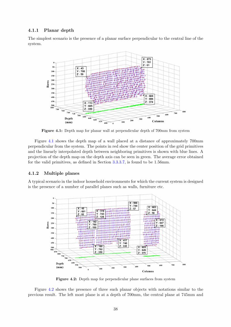
4.1.1 Planar depth
The simplest scenario is the presence of a planar surface perpendicular to the central line of thesystem.
Figure 4.1: Depth map for planar wall at perpendicular depth of 700mm from system
Figure 4.1 shows the depth map of a wall placed at a distance of approximately 700mmperpendicular from the system. The points in red show the center position of the grid primitivesand the linearly interpolated depth between neighboring primitives is shown with blue lines. Aprojection of the depth map on the depth axis can be seen in green. The average error obtainedfor the valid primitives, as defined in Section 3.3.3.7, is found to be 1.56mm.
4.1.2 Multiple planes
A typical scenario in the indoor household environments for which the current system is designedis the presence of a number of parallel planes such as walls, furniture etc.
Figure 4.2: Depth map for perpendicular plane surfaces from system
Figure 4.2 shows the presence of three such planar objects with notations similar to theprevious result. The left most plane is at a depth of 700mm, the central plane at 745mm and
38
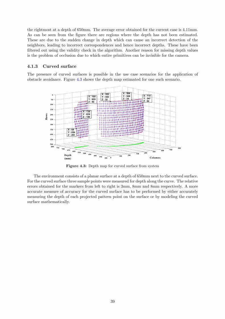
the rightmost at a depth of 650mm. The average error obtained for the current case is 4.11mm.As can be seen from the figure there are regions where the depth has not been estimated.These are due to the sudden change in depth which can cause an incorrect detection of theneighbors, leading to incorrect correspondences and hence incorrect depths. These have beenfiltered out using the validity check in the algorithm. Another reason for missing depth valuesis the problem of occlusion due to which entire primitives can be invisible for the camera.
4.1.3 Curved surface
The presence of curved surfaces is possible in the use case scenarios for the application ofobstacle avoidance. Figure 4.3 shows the depth map estimated for one such scenario.
Figure 4.3: Depth map for curved surface from system
The environment consists of a planar surface at a depth of 650mm next to the curved surface.For the curved surface three sample points were measured for depth along the curve. The relativeerrors obtained for the markers from left to right is 3mm, 8mm and 8mm respectively. A moreaccurate measure of accuracy for the curved surface has to be performed by either accuratelymeasuring the depth of each projected pattern point on the surface or by modeling the curvedsurface mathematically.
39
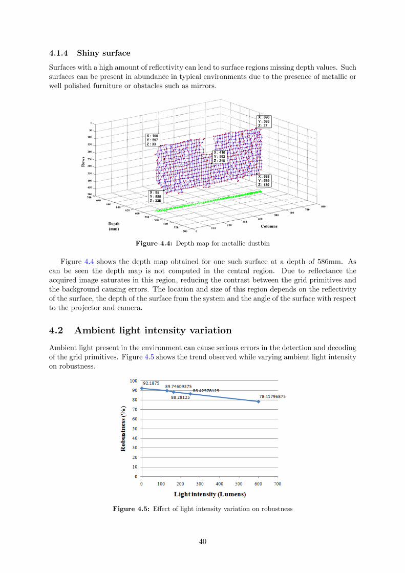
4.1.4 Shiny surface
Surfaces with a high amount of reflectivity can lead to surface regions missing depth values. Suchsurfaces can be present in abundance in typical environments due to the presence of metallic orwell polished furniture or obstacles such as mirrors.
Figure 4.4: Depth map for metallic dustbin
Figure 4.4 shows the depth map obtained for one such surface at a depth of 586mm. Ascan be seen the depth map is not computed in the central region. Due to reflectance theacquired image saturates in this region, reducing the contrast between the grid primitives andthe background causing errors. The location and size of this region depends on the reflectivityof the surface, the depth of the surface from the system and the angle of the surface with respectto the projector and camera.
4.2 Ambient light intensity variation
Ambient light present in the environment can cause serious errors in the detection and decodingof the grid primitives. Figure 4.5 shows the trend observed while varying ambient light intensityon robustness.
Figure 4.5: Effect of light intensity variation on robustness
40
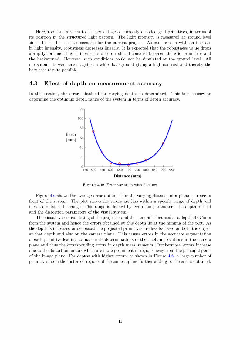
Here, robustness refers to the percentage of correctly decoded grid primitives, in terms ofits position in the structured light pattern. The light intensity is measured at ground levelsince this is the use case scenario for the current project. As can be seen with an increasein light intensity, robustness decreases linearly. It is expected that the robustness value dropsabruptly for much higher intensities due to reduced contrast between the grid primitives andthe background. However, such conditions could not be simulated at the ground level. Allmeasurements were taken against a white background giving a high contrast and thereby thebest case results possible.
4.3 Effect of depth on measurement accuracy
In this section, the errors obtained for varying depths is determined. This is necessary todetermine the optimum depth range of the system in terms of depth accuracy.
Figure 4.6: Error variation with distance
Figure 4.6 shows the average error obtained for the varying distance of a planar surface infront of the system. The plot shows the errors are less within a specific range of depth andincrease outside this range. This range is defined by two main parameters, the depth of fieldand the distortion parameters of the visual system.
The visual system consisting of the projector and the camera is focussed at a depth of 675mmfrom the system and hence the errors obtained at this depth lie at the minima of the plot. Asthe depth is increased or decreased the projected primitives are less focussed on both the objectat that depth and also on the camera plane. This causes errors in the accurate segmentationof each primitive leading to inaccurate determinations of their column locations in the cameraplane and thus the corresponding errors in depth measurements. Furthermore, errors increasedue to the distortion factors which are more prominent in regions away from the principal pointof the image plane. For depths with higher errors, as shown in Figure 4.6, a large number ofprimitives lie in the distorted regions of the camera plane further adding to the errors obtained.
41
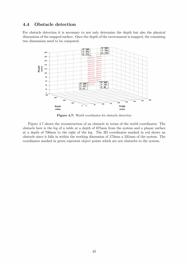
4.4 Obstacle detection
For obstacle detection it is necessary to not only determine the depth but also the physicaldimensions of the mapped surface. Once the depth of the environment is mapped, the remainingtwo dimensions need to be computed.
Figure 4.7: World coordinates for obstacle detection
Figure 4.7 shows the reconstruction of an obstacle in terms of the world coordinates. Theobstacle here is the leg of a table at a depth of 675mm from the system and a planar surfaceat a depth of 700mm to the right of the leg. The 3D coordinates marked in red shows anobstacle since it falls in within the working dimension of 173mm x 331mm of the system. Thecoordinates marked in green represent object points which are not obstacles to the system.
42
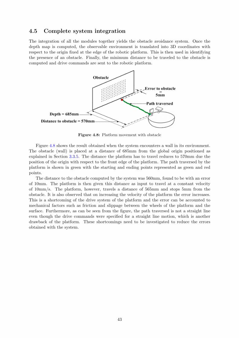
4.5 Complete system integration
The integration of all the modules together yields the obstacle avoidance system. Once thedepth map is computed, the observable environment is translated into 3D coordinates withrespect to the origin fixed at the edge of the robotic platform. This is then used in identifyingthe presence of an obstacle. Finally, the minimum distance to be traveled to the obstacle iscomputed and drive commands are sent to the robotic platform.
Figure 4.8: Platform movement with obstacle
Figure 4.8 shows the result obtained when the system encounters a wall in its environment.The obstacle (wall) is placed at a distance of 685mm from the global origin positioned asexplained in Section 3.3.5. The distance the platform has to travel reduces to 570mm due theposition of the origin with respect to the front edge of the platform. The path traversed by theplatform is shown in green with the starting and ending points represented as green and redpoints.
The distance to the obstacle computed by the system was 560mm, found to be with an errorof 10mm. The platform is then given this distance as input to travel at a constant velocityof 10mm/s. The platform, however, travels a distance of 565mm and stops 5mm from theobstacle. It is also observed that on increasing the velocity of the platform the error increases.This is a shortcoming of the drive system of the platform and the error can be accounted tomechanical factors such as friction and slippage between the wheels of the platform and thesurface. Furthermore, as can be seen from the figure, the path traversed is not a straight lineeven though the drive commands were specified for a straight line motion, which is anotherdrawback of the platform. These shortcomings need to be investigated to reduce the errorsobtained with the system.
43
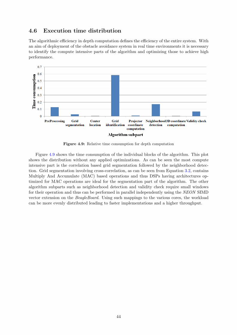
4.6 Execution time distribution
The algorithmic efficiency in depth computation defines the efficiency of the entire system. Withan aim of deployment of the obstacle avoidance system in real time environments it is necessaryto identify the compute intensive parts of the algorithm and optimizing those to achieve highperformance.
Figure 4.9: Relative time consumption for depth computation
Figure 4.9 shows the time consumption of the individual blocks of the algorithm. This plotshows the distribution without any applied optimizations. As can be seen the most computeintensive part is the correlation based grid segmentation followed by the neighborhood detec-tion. Grid segmentation involving cross-correlation, as can be seen from Equation 3.2, containsMultiply And Accumulate (MAC) based operations and thus DSPs having architectures op-timized for MAC operations are ideal for the segmentation part of the algorithm. The otheralgorithm subparts such as neighborhood detection and validity check require small windowsfor their operation and thus can be performed in parallel independently using the NEON SIMDvector extension on the BeagleBoard. Using such mappings to the various cores, the workloadcan be more evenly distributed leading to faster implementations and a higher throughput.
44
CHAPTER 5
Conclusion and Future Work
This thesis details the design and implementation of an obstacle avoidance system for a roboticvacuum cleaner prototype using embedded components. It is based on the principle of depthestimation using the active vision technique of structured light. This structured light basedsystem shows accurate depth estimation over a range of surface objects under varying ambientlight conditions which shows its advantages over the conventional stereoscopic vision baseddepth estimation. It is able to estimate the depth of an obstacle with upto 10mm accuracy forobstacle depths ranging from 600 to 800mm and is able to determine the presence of an obstacleof size 20mm x 18mm at a projection distance of 675mm. This is found to be adequate for anumber of real world obstacles, expected to be encountered by a vacuum cleaning system. Theresults obtained using the current system also demonstrate that by using a simplified calibrationprocedure and principle, depth can be accurately measured and obstacles can be detected.
For the design of a mobile obstacle avoidance system, the components selected need to beembedded in nature. The entire system consists of a robotic platform, a visual system to providethe depth information input, and an embedded computing unit to analyze the input and givedrive commands to the platform. The robotic platform selected was the Create from iRobotwhich allows navigation based on the reception of drive commands through a serial interface. Itis found to be accurate to distance commands at low drive velocity but this accuracy decreaseswith an increase in drive velocity. The visual system consists of a Pico projector from TexasInstruments that allows an easy construction of any desired projection pattern and a µEyeUSB camera from iDS that gives more control over its internal parameters. The embeddedcomputing unit selected for the current project is the BeagleBoard by Texas Instruments whichcontains peripheral connections to interface with all the other components of the system andhardware to satisfy the performance needs. The OS was selected based on the availability ofcompatible drivers for the camera. The placement of the visual system on the robot platformwas another critical aspect of the system design with the finalized system setup as shown inFigure 3.5.
The selection of the structured light pattern marks another critical aspect of the systemdesign with the pattern defining the robustness and the accuracy with which an obstacle isdetected. The pattern finally selected is shown in Figure 2.10. It is a two-dimensional andspatially multiplexed pattern to enable motion robustness, and binary in pixel depth to workin color non-neutral environments. The pattern is absolute- neighborhood coded with spatialprimitives and a small neighborhood to allow for a unique identification of all pattern pointswhich minimizes surface discontinuity errors
45
Future works
The main drawback of the current system is the repeated need for calibration. This hap-pens due to the unstable nature of the projector and camera mountings which change theirorientation due to any applied forces. A simple solution to this problem is the use of fixedmountings instead of the variable ones used in the current development setup.
To improve the performance of the entire system the algorithm can be split and distributedon multiples cores. The correlation based grid segmentation can be performed on the DSP coreoptimized for such operations. The neighborhood detection and the validity check operationsare based on individual windows and thus can be performed in parallel on the SIMD vectorextension for ARM using the provided NEON instruction set available on the BeagleBoard.Using an efficient algorithm mapping on such a heterogenous architecture can provide ordersof magnitude improvement in the algorithm implementation and such mappings need to beinvestigated for an increased throughput for the entire system.
Results show a reduction in robustness of the current system with an increase in the ambientlight in the observable environment. A possible solution to improving the robustness is by usingan Infrared (IR) visual system. However, IR wavelengths are also present in ambient light andcan be emitted by other sources present in the environments the current system is aimed for.Hence, the use of imaging at different light spectrum needs to be investigated with an aim toimprove the robustness of the entire system.
Another aspect which can be investigated is the use of a higher resolution visual system. Ahigher resolution projector will be capable of projecting finer patterns reducing the individualsize of the primitives, thereby reducing the decoding window size and thus the shape disconti-nuity errors giving a more accurate object mapping along its edges. A higher resolution visualsystem also promises to increase the spatial resolution of the system allowing the depth map-ping of smaller obstacles. However, the need of increasing the spatial resolution depends on thedefinition of an obstacle which in turn depends on the application.
46
Bibliography
[1] D. De Silva, W. Fernando, S. Worrall, and A. Kondoz, “A novel depth map quality metricand its usage in depth map coding,” in 3DTV Conference: The True Vision - Capture,Transmission and Display of 3D Video (3DTV-CON), 2011, may 2011, pp. 1 –4.
[2] C.-H. Kuo, H.-W. Yeh, and C.-E. Wu, “Development of autonomous navigation roboticwheelchairs using programmable system-on-chip based distributed computing architec-ture,” in Systems, Man and Cybernetics, 2007. ISIC. IEEE International Conference on,oct. 2007, pp. 2939 –2944.
[3] M. Goebl, M. Althoff, M. Buss, G. Farber, F. Hecker, B. Heissing, S. Kraus, R. Nagel,F. Leon, F. Rattei, M. Russ, M. Schweitzer, M. Thuy, C. Wang, and H. Wuensche, “Designand capabilities of the munich cognitive automobile,” in Intelligent Vehicles Symposium,2008 IEEE, june 2008, pp. 1101 –1107.
[4] P.-C. Hsieh and W. jong Kim, “Autonomous robotic wheelchair with collision-avoidancenavigation and real-time path planning,” in Advanced Intelligent Mechatronics (AIM), 2010IEEE/ASME International Conference on, july 2010, pp. 1396 –1401.
[5] D. Sales, P. Shinzato, G. Pessin, D. Wolf, and F. Osorio, “Vision-based autonomous navi-gation system using ann and fsm control,” in Robotics Symposium and Intelligent RoboticMeeting (LARS), 2010 Latin American, oct. 2010, pp. 85 –90.
[6] “Autonomous robotic vacuum cleaner,” Samsung, 2009. [Online]. Available: http://en.wikipedia.org/wiki/Samsung Navibot
[7] “Autonomous robotic vacuum cleaner,” iCreate, 2009. [Online]. Available: http://en.wikipedia.org/wiki/Roomba
[8] “Roomba - how it works,” iCreate. [Online]. Available: http://resources.irobot.com/index.php/howitworks/US/3881236
[9] “Kinect,” Microsoft, 2010. [Online]. Available: http://www.xbox.com/en-US/kinect
[10] Z. Z. et al., “Method and system for object reconstruction,” Patent US 60/724,903,November 10, 2005. [Online]. Available: http://www.wipo.int/pctdb/en/wo.jsp?WO=2007043036&IA=IL2006000335&DISPLAY=DESC
[11] K. Konolige and P. Mihelich, “Technical description of kinect calibration.” [Online].Available: http://www.ros.org/wiki/kinect calibration/technical
47
[12] B. F. et al., “Depth mapping using projected patterns,” Patent US 61/016,832,December 27, 2007. [Online]. Available: http://www.wipo.int/pctdb/en/wo.jsp?WO=2008120217&IA=IL2008000458&DISPLAY=DESC
[13] E. Mouaddib, J. Batlle, and J. Salvi, “Recent progress in structured light in order tosolve the correspondence problem in stereovision,” in Robotics and Automation, 1997.Proceedings., 1997 IEEE International Conference on, vol. 1, apr 1997, pp. 130 –136 vol.1.
[14] Y. Jianxi, Q. Jinwu, Y. Juxia, and F. Zengliang, “Research on computer aided surgicalnavigation based on binocular stereovision,” in Mechatronics and Automation, Proceedingsof the 2006 IEEE International Conference on, june 2006, pp. 1532 –1536.
[15] E. Olaya and L. Torres-Mendez, “A foveated stereo vision system for active depth per-ception,” in Robotic and Sensors Environments, 2009. ROSE 2009. IEEE InternationalWorkshop on, nov. 2009, pp. 110 –115.
[16] W. Chuan-xu and S. Ying-he, “A new method of depth measurement with binocular visionbased on surf,” in Computer Science and Engineering, 2009. WCSE ’09. Second Interna-tional Workshop on, vol. 1, oct. 2009, pp. 568 –571.
[17] E. Hall, J. Tio, C. McPherson, and F. Sadjadi, “Measuring curved surfaces for robotvision,” Computer, vol. 15, no. 12, pp. 42 – 54, dec 1982.
[18] “Euler angles.” [Online]. Available: http://en.wikipedia.org/wiki/Euler angles
[19] J. M. D. F. G. Falcao, N. Hurtos, “Projector-camera calibration toolbox,” 2009. [Online].Available: http://code.google.com/p/procamcalib/
[20] S. Narasimhan and S. Nayar, “Structured light methods for underwater imaging: lightstripe scanning and photometric stereo,” in OCEANS, 2005. Proceedings of MTS/IEEE,2005, pp. 2610 – 2617 Vol. 3.
[21] R. Benveniste and C. Unsalan, “Single stripe projection based range scanning of shinyobjects under ambient light,” in Computer and Information Sciences, 2009. ISCIS 2009.24th International Symposium on, sept. 2009, pp. 1 –6.
[22] B. Carrihill and R. Hummel, “Experiments with the intensity ratio depth sensor,”Computer Vision, Graphics, and Image Processing, vol. 32, no. 3, pp. 337 – 358, 1985.[Online]. Available: http://www.sciencedirect.com/science/article/pii/0734189X85900568
[23] M. Maruyama and S. Abe, “Range sensing by projecting multiple slits with random cuts,”Pattern Analysis and Machine Intelligence, IEEE Transactions on, vol. 15, no. 6, pp. 647–651, jun 1993.
[24] F. S.Inokuchi, K.Sato, “Range imaging system for 3d object recognition,” Proceedings ofthe international conference on pattern recognition, pp. 806–808, 1984.
[25] O. H.-H. Szymon, “Stripe boundary codes for real-time structured-light range scanningof moving objects,” 2001. [Online]. Available: http://alexandria.tue.nl/repository/books/252901.pdf
[26] J. POSDAMER and M. ALTSCHULER, “Surface measurement by space-encoded pro-jected beam systems,” Graphical Models /graphical Models and Image Processing /com-puter Vision, Graphics, and Image Processing, vol. 18, pp. 1–17, 1982.
[27] M. Minou, T. Kanade, and T. Sakai, “A method of time-coded parallel planes of lightfor depth measurement,” Trans. Institute of Electronics and Communication Engineers ofJapan, vol. E64, no. 1, pp. 521–528, August 1981.
48
[28] B. A. M.D. Altschuler and J.Taboada, “Laser electro-optic system for rapid three-dimensional (3d) topographic mapping of surfaces,” Optical engineering, vol. 20, pp. 953–961, 1981.
[29] N. Durdle, J. Thayyoor, and V. Raso, “An improved structured light technique for surfacereconstruction of the human trunk,” in Electrical and Computer Engineering, 1998. IEEECanadian Conference on, vol. 2, may 1998, pp. 874 –877 vol.2.
[30] M. Ito and A. Ishii, “A three-level checkerboard pattern (tcp) projection method for curvedsurface measurement,” Pattern Recognition, vol. 28, pp. 27–40, 1995.
[31] K. L. Boyer and A. C. Kak, “Color-encoded structured light for rapid active ranging,”Pattern Analysis and Machine Intelligence, IEEE Transactions on, vol. PAMI-9, no. 1, pp.14 –28, jan. 1987.
[32] C.-S. Chen, Y.-P. Hung, C.-C. Chiang, and J.-L. Wu, “Range data acquisition using colorstructured lighting and stereo vision.” Image Vision Comput.
[33] N. Bruijn, “Acknowledgement of priority to c. flye sainte-marie on the countingof circular arrangements of 2n zeros and ones that show each n-letter wordexactly once,” Eindhoven University of Technology, 1975. [Online]. Available:http://alexandria.tue.nl/repository/books/252901.pdf
[34] B. Arazi, “Method of constructing de-bruijn sequences,” Electronics Letters, vol. 12, no. 25,pp. 658 –659, 9 1976.
[35] C. Wust and D. W. Capson, “Surface profile measurement using color fringe projection,”Machine Vision and Applications, vol. 4, pp. 193–203, 1991, 10.1007/BF01230201.[Online]. Available: http://dx.doi.org/10.1007/BF01230201
[36] J. Tajima and M. Iwakawa, “3d data acquisition by rainbow range finder,” in InternationalConference on pattern recognition, 1990, pp. 309–313.
[37] P. M. Griffin, L. S. Narasimhan, and S. R. Yee, “Generation of uniquely encoded lightpatterns for range data acquisition,” Pattern Recognition, vol. 25, no. 6, pp. 609 – 616, 1992.[Online]. Available: http://www.sciencedirect.com/science/article/pii/003132039290078W
[38] C. Rocchini, P. Cignoni, C. Montani, P. Pingi, and R. Scopigno, “A low cost 3d scannerbased on structured light,” 2001.
[39] N. Durdle, J. Thayyoor, and V. Raso, “An improved structured light technique for surfacereconstruction of the human trunk,” in Electrical and Computer Engineering, 1998. IEEECanadian Conference on, vol. 2, may 1998, pp. 874 –877 vol.2.
[40] Y.-C. Hsieh, “A note on the structured light of three-dimensional imaging systems,”Pattern Recognition Letters, vol. 19, no. 3-4, pp. 315 – 318, 1998. [Online]. Available:http://www.sciencedirect.com/science/article/pii/S0167865597001591
[41] Y. chih Hsieh, “Decoding structured light patterns for three-dimensional imaging systems,”Pattern Recognition, vol. 34, pp. 343–349, 2001.
[42] “Beagleboard,” Texas Instruments. [Online]. Available: http://beagleboard.org
[43] “Beagleboard demo image,” The Angstrom distribution. [Online]. Available: http://www.angstrom-distribution.org/beagleboard-demo-image-available
[44] “Create,” iRobot, 2007. [Online]. Available: http://resources.irobot.com/index.php/global
49

[45] “Using the dlp pico2.0 kit for structured light applications,” Texas Instruments, January2010. [Online]. Available: http://focus.ti.com/lit/an/dlpa021/dlpa021.pdf
[46] J. Thompson, Pico-Projector Development Kit Programmer’s Guide, Texas Instruments,august 2009. [Online]. Available: http://www.dlinnovations.com/doc/PicoKitGuide.pdf
[47] Z. Zhang, “A flexible new technique for camera calibration,” IEEE Transactions onPattern Analysis and Machine Intelligenc, vol. 22, no. 11, pp. 1330–1334, 2000. [Online].Available: http://research.microsoft.com/en-us/um/people/zhang/papers/TR98-71.pdf
[48] J. Bouguet, “Camera calibration toolboxfor matlab,” July 2010. [Online]. Available:http://www.vision.caltech.edu/bouguetj/calib doc/
[49] G. Bradski and A. Kaehler, Learning OpenCV - Computer Vision with the OpenCV Library.O’Reilly, 2008.
50