3D MODELING OF SALT RELATED STRUCTURES

IN THE FRIESLAND PLATFORM, THE NETHERLANDS

A THESIS SUBMITTED TO

THE GRADUATE SCHOOL OF NATURAL AND APPLIED SCIENCES

OF

MIDDLE EAST TECHNICAL UNIVERSITY

BY

KIVANÇ YÜCEL

IN PARTIAL FULFILLMENT OF THE REQUIREMENTS

FOR

THE DEGREE OF MASTER OF SCIENCE

IN

GEOLOGICAL ENGINEERING

JULY 2010

Approval of the thesis:

3D MODELING OF SALT RELATED STRUCTURES IN THE FRIESLAND

PLATFORM, THE NETHERLANDS

submitted by KIVANÇ YÜCEL in partial fulfillment of the requirements for the degree

of Master of Science in Geological Engineering Department, Middle East Technical

University by,

Prof. Dr. Canan Özgen

Dean, Graduate School of Natural and Applied Sciences _________________

Prof. Dr. Zeki Çamur

Head of Department, Geological Engineering _________________

Assoc. Prof. Dr. Nuretdin Kaymakcı

Supervisor, Geological Engineering Dept., METU _________________

Assist. Prof. Dr. A. Arda Özacar

Co-Supervisor, Geological Engineering Dept., METU _________________

Examining Committee Members:

Prof. Dr. Erdin Bozkurt

Geological Engineering Dept., METU _________________

Assoc. Prof. Dr. Nuretdin Kaymakcı

Geological Engineering Dept., METU _________________

Assist. Prof. Dr. A. Arda Özacar

Geological Engineering Dept., METU _________________

Dr. Özgür Sipahioğlu

Turkish Petroleum Corporation _________________

Dr. Sadun Arzuman

Schlumberger , TURKEY _________________

Date: 19.07.2010

iii

I hereby declare that all information in this document has been obtained and

presented in accordance with academic rules and ethical conduct. I also declare that,

as required by these rules and conduct, I have fully cited and referenced all material

and results that are not original to this work.

Name, Last name: Kıvanç Yücel

Signature:

iv

ABSTRACT

3D MODELING OF SALT RELATED STRUCTURES IN THE FRIESLAND

PLATFORM, THE NETHERLANDS

Yücel, Kıvanç

M.Sc., Department of Geological Engineering

Supervisor: Assoc. Prof. Dr. Nuretdin Kaymakcı

Co-Supervisor: Assist. Prof. Dr. A. Arda Özacar

July 2010, 78 pages

Southern North Sea Basin is one of the mature hydrocarbon basins in NW Europe and

is shaped by a number of phases of tectonic deformations during the Phanerozoic. In

addition, mobilization and halokinesis of thick Permian Zechstein Salt has enhanced

and contributed to the deformation of the region since Triassic, which further

complicated the geology of the region. The Friesland Platform, which is a stable

platform area located in northern Netherlands, experienced the main deformation

phases that Europe has been endured together with the deformation of Permian

Zechstein salt.

In this study a computer based 3D modeling has been carried out within the Friesland

Platform with the use of 3D seismic and borehole data in order to delineate structural

elements and geological development of the area with special emphasis on the salt

tectonic deformation.

The model was constructed by picking key horizons and major faults from the seismic

sections in time domain and then migrated into depth domain. The stratigraphy of the

area is correlated with horizons by well-seismic matching.

v

The model includes major structures and seismostratigraphic units of Permian to

recent, revealing salt and salt induced structures formed during the periods of active

salt movements. Thick Zechstein salt layers deposited in N-S-oriented grabens and half

grabens of South Permian Basin acted as the primary control for the location of salt

diapirs and are reflected on the overburden without a direct continuation (unlinked) of

the basement faults into the overburden. The mapped N-S oriented salt-cored anticline

and a convergent conjugate transfer zone between a pair of segmented normal growth

faults at the crest of the anticline are controlled by the ascent of the Zechstein salt.

Keywords: 3D solid modeling, 3D seismics, salt tectonics, transfer fault, Friesland

Platform, the Netherlands.

vi

ÖZ

HOLLANDA, FRIESLAND PLATFORMUNDAKİ TUZ YAPILARININ 3 BOYUTLU

MODELLEMESİ

Yücel, Kıvanç

Yüksek Lisans, Jeoloji Mühendisliği Bölümü

Tez Yöneticisi: Doç. Dr. Nuretdin Kaymakcı

Ortak Tez Yöneticisi: Yrd. Doç. Dr. A. Arda Özacar

Temmuz 2010, 78 sayfa

Güney Kuzey Denizi havzası, kuzeybatı Avrupa’da bulunan ve çeşitli Fanerozoik

tektonik deformasyonlarla şekillenmiş hidrokarbon havzalarından birisidir. Buna ek

olarak Permiyen Zecshstein tuzunun Trias’la başlayan hareketlenmesi ve halokinesi ile

bölgedeki deformasyon daha da karmaşık bir hal almıştır. Friesland Platformu, kuzey

Hollanda’da sabit bir platform olarak Avrupa’nın tuz deformasyonu dahilinde, bu ana

deformasyon fazlarından etkilenmiştir.

Bölgede 3 boyutlu sismik ve kuyu verileri kullanılarak bilgisayar tabanlı 3 boyutlu

modelleme yapılması ve tuz deformasyonu başta olmak üzere bölgenin jeolojik

geçmişinin yorumlanması amaçlanmıştır.

Model fay ve stratigrafik katmanların zaman tabanlı sismik kesitlerde yorumlanması ve

zamandaki modelin derinliğe göçü ile oluşturulmuştur. Bölgenin stratigrafisinin

sismiklerle korelasyonu kuyu verisi ile yapılmıştır.

Model ana jeolojik yapılar ve sismik stratigrafik birimleri içermektedir. Böylece tuz ve

tuz ilişkili yapıları ortaya koyarak bölgenin Permiyen’den günümüze kadar olan aktif

tuz deformasyonu ortaya çıkartılmıştır. Kalın Zechstein tuz tabakası Güney Permiyen

Havzası’nda, kuzey-güney uzanımlı graben ve yarı-graben yapılarının üzerine

vii

depolanmıştır. Bu graben yapıları tuz domlarının aynı şekilde kuzey güney yönünde

oluşmasını da tetiklemiştir. Çekirdeğinde tuz bulunan kuzey-güney uzanımlı antiklinal

ile yöndeşik transfer zonu, tuz hareketiyle kontrol edilmiştir. Bu durum doğrudan bir

bağlantı olmamasına rağmen, taban faylarının, yüzeysel yapıların yönelimini kontrol

ettiğini ortaya çıkarmıştır.

Anahtar kelimeler: 3 boyutlu modelleme, 3 boyutlu sismik, tuz tektoniği, transfer fayı,

Friesland Platformu, Hollanda

viii

To My Parents

ix

ACKNOWLEDGEMENTS

I am deeply grateful to my supervisor Assoc. Prof. Dr. Nuretdin Kaymakcı for his

invaluable guidance, encouragement and continued advice throughout the course of

my M.Sc. studies. It is an honor for me to work with him.

I would like to thank to my co-supervisor Assist. Prof. Dr. A. Arda Özacar for his

valuable guidance, continued advice and critical discussion throughout this study.

I wish to thank my examining committee members, Prof. Dr. Erdin Bozkurt, Dr. Özgür

Sipahioğlu and Dr. Sadun Arzuman for their valuable recommendations and criticism.

Special thanks are extended to Dr. Sadun Arzuman from whom I have learned a lot

before and throughout the study, especially with his theoretical support in using Petrel

software. In addition, I would like to thank Schlumberger for Petrel availability.

I am heartily thankful to my friends especially my roommate Ezgi Karasözen, structural

geology team; Ayten Koç, Erhan Gülyüz, Murat Özkaptan and also A. Mert Eker, Selim

Cambazoğlu and Çiğdem Cankara for their support, friendship and endless

encouragement throughout this study. It was enjoyable to work with them.

I am also grateful to my family for their patience, permanent encouragement and belief

in me throughout this work.

Finally, I wish to express my deepest thanks to Duygu Yılmaz for her guidance,

patience, care and love. This thesis belongs to her as much as it belongs to me. Her

confidence on me gave me all the strength and courage I need to complete this work.

x

TABLE OF CONTENTS

ABSTRACT ............................................................................................................................... iv

ÖZ ............................................................................................................................................... vi

ACKNOWLEDGEMENTS ..................................................................................................... ix

TABLE OF CONTENTS ........................................................................................................... x

LIST OF TABLES ................................................................................................................... xiii

LIST OF FIGURES ................................................................................................................. xiv

LIST OF ABBREVIATIONS .............................................................................................. xviii

CHAPTER

1. INTRODUCTION .................................................................................................................. 1

1.1 Purpose and Scope ............................................................................................................ 1

1.2 Study Area ......................................................................................................................... 2

1.3 Data and Methods of Study ............................................................................................. 3

1.4 Previous Works ................................................................................................................. 4

2. GEOLOGICAL SETTING .................................................................................................... 7

2.1 Regional Geological Setting ............................................................................................. 7

2.1.1 Paleozoic Tectonics: Caledonian and Variscan Events ......................................... 8

2.1.2 Mesozoic Events: Break-up of Pangea .................................................................. 10

2.1.3 Late Cretaceous – Early Tertiary Evolution: Alpine Orogeny ........................... 11

2.1.4 Early Tertiary – Recent Evolution: Rhine Graben Rifting .................................. 12

2.2 Geology of the Study Area ............................................................................................. 12

2.2.1 Tectonic Setting ........................................................................................................ 12

2.2.2 Stratigraphy .............................................................................................................. 13

2.2.2.1 Upper Rotliegend Group (RO) (Middle to Late Permian) .......................... 18

xi

2.2.2.2 Zechstein Group (ZE) (Late Permian) ............................................................ 19

2.2.2.3 Germanic Trias Supergroup (T) (Triassic) ..................................................... 19

2.2.2.4 Rjinland Group (KN) (Early Cretaceous)....................................................... 20

2.2.2.5 Chalk Group (CK) (Late Cretaceous - Early Paleocene) .............................. 22

2.2.2.6 North Sea Supergroup (NS) (Tertiary - Recent) ............................................ 22

3. SEISMIC INTERPRETATION AND MODELING ....................................................... 23

3.1 Modeling Concept and Workflow ................................................................................ 23

3.2 Seismic Interpretation ..................................................................................................... 25

3.2.1 Defining and Picking the Key Horizons ............................................................... 25

3.2.2 Surface Generation ................................................................................................... 29

3.2.3 Fault Interpretation .................................................................................................. 30

3.3 Structural Modeling ........................................................................................................ 31

3.3.1 Fault Modeling ......................................................................................................... 31

3.3.2 Pillar Gridding .......................................................................................................... 32

3.3.3 Generation of Faulted Horizons ............................................................................ 33

3.4 Velocity Models and Depth Conversion ...................................................................... 35

3.4.1 Constant (Interval) Velocity Model ....................................................................... 35

3.4.2 Vok Method ............................................................................................................... 36

3.4.3 Assessment of the Velocity Models ....................................................................... 36

4. RESULTS ............................................................................................................................... 39

4.1 Model Outputs ................................................................................................................ 39

4.2 Characteristics of Seismic-Stratigraphic Units ............................................................ 44

4.2.1 Permian: Zechstein Group ...................................................................................... 44

4.2.2 Triassic: Germanic Trias Supergroup .................................................................... 44

4.2.3 Cretaceous: Rjinland and Chalk Groups .............................................................. 45

4.2.4 Cenozoic: North Sea Supergroup .......................................................................... 45

4.3 Evaluation of structures ................................................................................................. 46

4.3.1 Unconformities ......................................................................................................... 46

4.3.2 Salt Structures ........................................................................................................... 48

xii

4.3.3 Faults .......................................................................................................................... 51

5. DISCUSSION AND CONCLUSIONS ............................................................................ 57

5.1 Structural Development and Salt Tectonics ................................................................ 57

5.2 Summary and Conclusions ............................................................................................ 62

REFERENCES ........................................................................................................................... 64

APPENDICES ........................................................................................................................... 67

A: Isopach Maps of the Seismic Stratigraphic Units ........................................................ 57

B: Interpreted Seismic Sections ........................................................................................... 74

xiii

LIST OF TABLES

TABLES

Table 3.1: Recognized stratigraphic units and corresponding picked horizons. ......... 29

Table 3.2: Parameters of velocity models for each stratigraphic unit. ........................... 36

xiv

LIST OF FIGURES

FIGURES

Figure 1.1: Location of the study area, overlaid on Google Earth image. ......................... 2

Figure 1.2: Seismic survey area with inline-crossline directions and well

distributions. Some of the wells are deviated, and originate from the

same location such as wells BLF 101, 102, 103, 104, 105, 106 and 107, and

indicated on the map as a single well location; BLF 101-107. .......................... 3

Figure 2.1: Major tectonic elements and basins in northwest Europe (modified from

van Buggenum & den Hartog Jager 2007 and Geluk 2007) SA: study

area. .......................................................................................................................... 8

Figure 2.2: a) Reservoir types and major structural elements of the Netherlands and

its surroundings. b) regional cross-section along line XY (modified from

De Jager, 2007). ....................................................................................................... 9

Figure 2.3: Location of well sections A, B and C. ................................................................ 13

Figure 2.4: Well section A (see Figure 2.3 for its location) ................................................. 14

Figure 2.5: Well section B (see Figure 2.3 for its location). ................................................. 15

Figure 2.6: Well section C (see Figure 2.3 for its location). ................................................ 16

Figure 2.7: Generalized columnar section of the study area (Compiled from de

Gans, 2007; Geluk, 2007a; Geluk, 2007b; Herngreen and Wong, 2007;

Wong et al., 2007) ................................................................................................. 17

Figure 2.8: Generalized Permian and Triassic lithostratigraphy in the Netherlands

(adopted from Geluk, 2007b; Herngreen & Wong, 2007; Wong et al,

2007) ....................................................................................................................... 18

Figure 2.9: Generalized post-Jurassic lithostratigraphical units of the Netherlands

(modified from Geluk 2007b). ............................................................................ 21

Figure 3.1: Flowchart of the modeling process. ................................................................... 24

xv

Figure 3.2: Well seismic correlation shown in a seismic line passing through 6

wells. Units NU, NM, NL, CK, KN, T and ZE can be matched with well

data (either directly or by matching thicknesses and observing shifts).

Note, that there are slight mismatches between well tops and horizons

below Cretaceous (KN). This is due to local interval velocity variations. ... 27

Figure 3.3: Close-up view of the anhydrite, clay and carbonate layers within the

Zechstein Group. .................................................................................................. 28

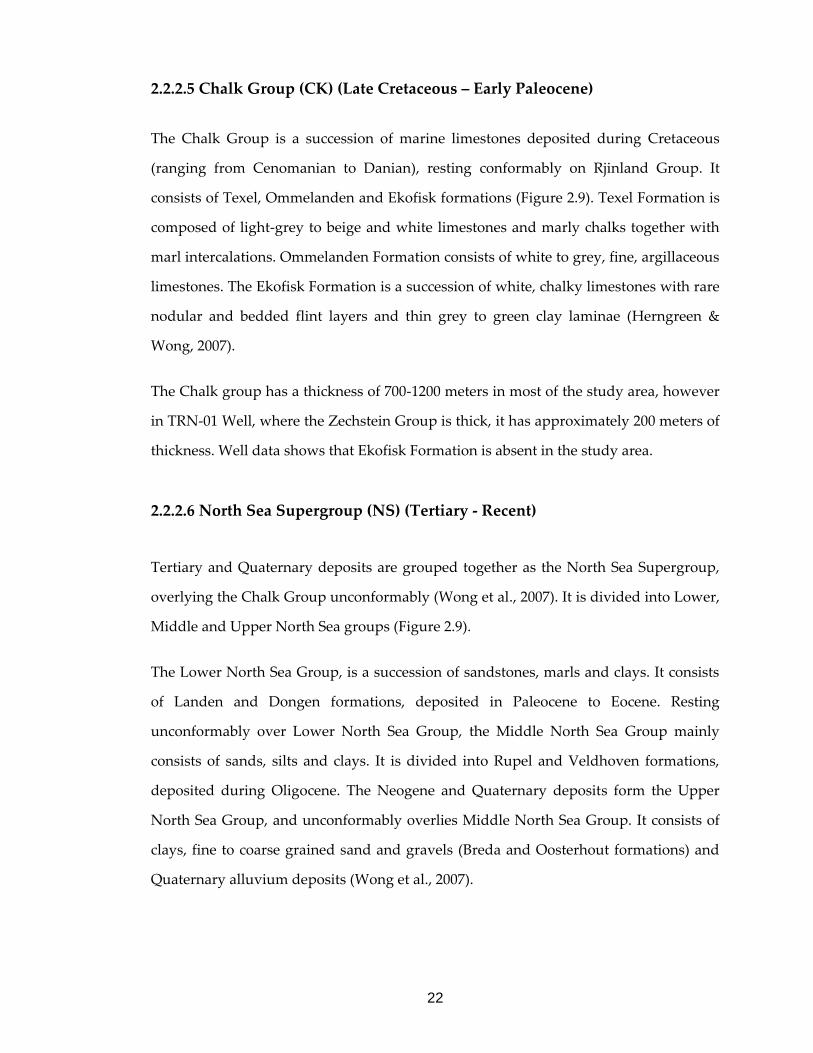
Figure 3.4: Picked horizons (left) are converted to surfaces in time domain (middle)

where surface attributes enable tracing of the faults (black lines). Then

seismic lines nearly perpendicular to the trends of the faults (right) are

used for accurate interpretation. ........................................................................ 30

Figure 3.5: Distribution of the interpreted faults (compare with figure 3.7) ................... 31

Figure 3.6: Map view of the faults that are chosen for fault modeling process in

which crossing faults are truncated (shown by arrows) and minor faults

which are insignificant for modeling process are eliminated.. ...................... 32

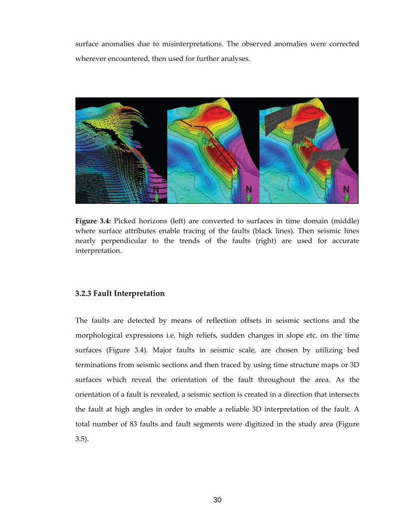
Figure 3.7: 3D view of top, middle and base grids with faults. ........................................ 33

Figure 3.8: Change of the displacement amount depending on the distance to fault

parameter. In this case small distance parameter (a) result in erroneous

fault displacement due to smearing (b,c) whereas a larger displacement

parameter (d) result in more accurate fault displacement (e,f). .................... 34

Figure 3.9: Correlation of depth converted surfaces with the well tops. Same cross

section, passing through 4 wells are used for cross-correlation of

velocity models. The mismatch error is higher in interval velocity model

(a) compared to Vok method which gives nearly perfect results (b) with

slight shift which is corrected with the well tops (c). ...................................... 38

Figure 4.1: Vertically (x4) exaggerated perspective view (a) and map view (b) of the

model with layers, faults and wells. .................................................................. 39

xvi

Figure 4.2: Isopach maps of the seismic stratigraphic units. White areas are zero

thickess zones. (D: depleted, E: eroded. Unmarked areas are the barren

zones due to faulting). See Appendices A1-A7 for higher resolution of

these figures. ......................................................................................................... 40

Figure 4.3: Interpreted and vertically (x5) exaggerated composite (arbitrary)

seismic section in time domain. ......................................................................... 42

Figure 4.4: Stratigraphic and structural interpretation of the composite seismic

section on Figure 4.3, showing major seismic stratigprahic units, faults

and unconformities. Section is cutting across the main salt cored

anticline (left) and dome shaped salt pillow (right). ....................................... 43

Figure 4.5: Unconformity within the Triassic units (green line) in the Triassic mini

basin and Base Cretaceous Unconformity (red line) above the Triassic

units (location shown in figure 4.3). .................................................................. 46

Figure 4.6: Early Miocene Unconformity (yellow line) above the crest of the salt

structure. Erosion is effective near the faults and crest where Middle

North Sea and Lower North Sea groups are extensively eroded (location

shown in figure 4.3). ............................................................................................ 48

Figure 4.7: Map view (left) and vertically exxagerated (3x) 3D perspective view of

top Zechstein, indicating the rise of the salt layer. .......................................... 50

Figure 4.8: Map view (left) and vertically (x3) exaggerated 3D perspective view

(right) of Base Zechstein, showing Permian faults and possible graben-

half graben structures. ......................................................................................... 52

Figure 4.9: Cross section A-B-C indicated on Figure 4.8. Manifestation of basement

(red) and overburden faults (blue). Note that the overburden faults do

not penetrate below the Zechstein (ZE). Note also that only major faults

are indicated. ......................................................................................................... 53

Figure 4.10: Map view (left) and vertically exaggerated (x3) 3D perspective view

(right) of Top Chalk showing Cenozoic faults, including master faults of

the convergent conjugate transfer zone. ........................................................... 54

xvii

Figure 4.11: W-E oriented (transverse to transfer zone) seismic sections (5x

exaggerated) in time domain showing seismic stratigraphic units and

convergent transfer zone with master faults and small scale antithetic

and synthetic faults. ............................................................................................. 55

Figure 4.12: Model representation of convergent conjugate transfer zone, showing

barren zones of the master faults at each Cenozoic surface (top), and 3D

perspective view of the transfer zone above the salt layer with master

faults and nearly perpendicular cross sections (bottom)................................ 56

Figure 5.1: Conceptual cartoon (not to scale) illustrating the structural and the

stratigraphical evolution of the study area. ...................................................... 61

Figure 5.2: Top CK, Top ZE and Base ZE surfaces showing the coinciding

orientation of basement graben-half graben system, salt pillow and

convergent conjugate transfer zone. .................................................................. 62

Figure A.1: Isopach map of Zechstein Group. D: salt depleted areas ............................... 67

Figure A.2: Isopach map of Germanic Trias Supergroup. E: eroded areas. ..................... 68

Figure A.3: Isopach map of Rjinland Group. ........................................................................ 69

Figure A.4: Isopach map of Chalk Group. ............................................................................ 70

Figure A.5: Isopach map of Lower North Sea Group. E: eroded areas. ............................ 71

Figure A.6: Isopach map of Middle North Sea Group E: eroded areas. ........................... 72

Figure A.7: Isopach map of Upper North Sea Group. ......................................................... 73

Figure B.1: Interpreted (top) and uninterpreted (bottom) seismic section A-A’. See

Figure 4.11 for its location ................................................................................... 74

Figure B.2: Interpreted (top) and uninterpreted (bottom) seismic section B-B’. See

Figure 4.11 for its location ................................................................................... 75

Figure B.3: Interpreted (top) and uninterpreted (bottom) seismic section C-C’. See

Figure 4.11 for its location ................................................................................... 76

Figure B.4: Interpreted (top) and uninterpreted (bottom) seismic section D-D’. See

Figure 4.11 for its location ................................................................................... 77

Figure B.5: Interpreted (top) and uninterpreted (bottom) seismic section E-E’. See

Figure 4.11 for its location ................................................................................... 78

xviii

LIST OF ABBREVIATIONS

CK: Chalk Group

DC: Limburg Group

KN: Rjinland Group

Ma: Millions of years

MB: Minibasin

MF: Master fault

NL1: Lower North Sea Unit 1

NL2: Lower North Sea Unit 2

NL3: Lower North Sea Unit 3

NM: Middle North Sea Group

NS: North Sea Supergroup

NU1: Upper North Sea Unit 1

NU2: Upper North Sea Unit 2

PK: Prekinematic

RB: Lower Germanic Trias Group

RN: Upper Germanic Trias Group

RO: Rotliegend Group

SA: Study Area

SK: Synkinematic

SSTVD: Sub sea true vertical depth

T: Germanic Trias Supergroup

TD: Total depth

ZE: Zechstein Group

1

CHAPTER 1

INTRODUCTION

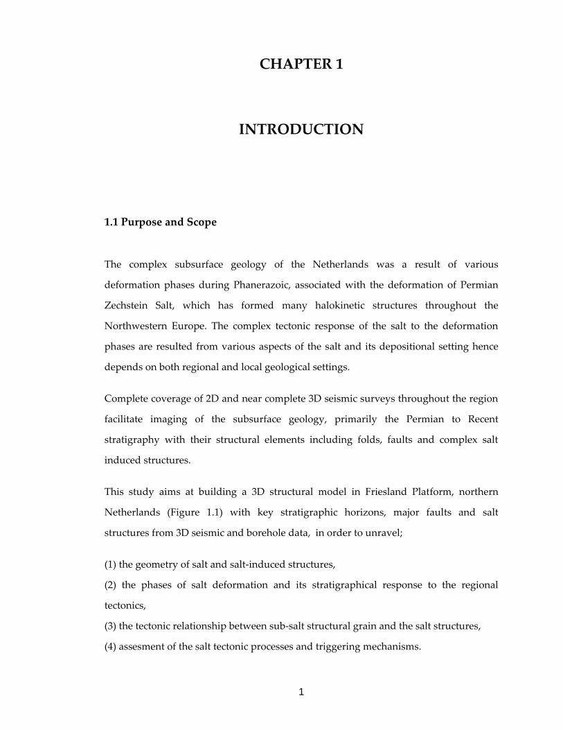
1.1 Purpose and Scope

The complex subsurface geology of the Netherlands was a result of various

deformation phases during Phanerazoic, associated with the deformation of Permian

Zechstein Salt, which has formed many halokinetic structures throughout the

Northwestern Europe. The complex tectonic response of the salt to the deformation

phases are resulted from various aspects of the salt and its depositional setting hence

depends on both regional and local geological settings.

Complete coverage of 2D and near complete 3D seismic surveys throughout the region

facilitate imaging of the subsurface geology, primarily the Permian to Recent

stratigraphy with their structural elements including folds, faults and complex salt

induced structures.

This study aims at building a 3D structural model in Friesland Platform, northern

Netherlands (Figure 1.1) with key stratigraphic horizons, major faults and salt

structures from 3D seismic and borehole data, in order to unravel;

(1) the geometry of salt and salt-induced structures,

(2) the phases of salt deformation and its stratigraphical response to the regional

tectonics,

(3) the tectonic relationship between sub-salt structural grain and the salt structures,

(4) assesment of the salt tectonic processes and triggering mechanisms.

2

1.2 Study Area

The study area is located in Ternaard field in the north of Friesland Province in

northern Netherlands. The exact location of the study area is defined by the seismic

survey coverage between latitudes 53.31° - 53.66° and longitudes 5.64° - 6.02°, covering

an area of approximately 900 km2 (Figure 1.1).

Figure 1.1: Location of the study area, overlaid on Google Earth image.

3

1.3 Data and Methods of Study

This thesis study was carried out at three main stages: (1) data collection and literature

survey, (2) computer-based modeling and (3) evaluation of the outcomes.

The data comprises; digital 3D seismic reflection data set data and well data. The

seismic dataset contains 1298 inlines and 1204 crosslines in which the inline and

crossline interval is 25 meters with sampling rate of 4 ms. Well data includes

lithostratigraphic units down to member rank. 33 wells exist throughout the study area

(Figure 1.2).

Figure 1.2: Seismic survey area with inline-crossline directions and well distributions.

Some of the wells are deviated, and originate from the same location such as wells BLF

101, 102, 103, 104, 105, 106 and 107, and indicated on the map as a single well location;

BLF 101-107.

4

Available literature has been collected and studied in detail, regarding the regional and

local geology. Apart from understanding the geology and tectonic evolution of the

region, literature information was used mainly for the selection of key horizons and

seismic stratigraphical units.

A computer-based 3D model has been constructed using PETREL 2008© “seismic to

simulation” software of Schlumberger Company. Model was constructed by picking

horizons and faults from seismic sections in time domain and then migrated into depth

domain using various time-to-depth conversion approaches. The 3D model is used to

build thickness maps of horizons and fault maps as well as 3D surface images that

facilitate the evaluation of structures and deformation styles of the study area.

1.4 Previous Works

This study is centered around the stratigraphic and structural development of northern

part of the Netherlands and southern North Sea Basin. The geology of the study area

reflects nearly all phases of the tectonic events in the Netherlands and its surrounding

region (Central European Basin) that has been endured, mainly during the much of the

Phanerozoic. This section gives a brief summary of the literature, concerning the studies

and researches that are used in this thesis.

The geology of the Netherlands has been studied by several authors since 1800’s. Due

to the fact that the surface sediments are mostly Quaternary in age, first studies include

only the distribution of younger sediments and compilation of small-scale geological

maps, with the help of shallow drillings and field observations (Wong et al., 2007). The

subsurface geology of the Netherlands has been revealed by exploration companies that

started in the 20th century and studied by many geoscientists since.

Overview of the geology and geological resources of the Netherlands was published by

several authors earliest of which include Pannekoek (1956), Heybroek (1974) and Van

Staalduinen et al. (1979). Among these, Ziegler (1988) is one of the most important

5

study and is dealt with structural history of the NW Europe and North Sea Basin area.

These works also commented on the early structural history of the region and include

mainly the Variscan orogenic and Late Variscan post-orogenic tectonics. According to

these studies, Variscan crustal shortening was terminated during the Late Westphalian

which are the main source rocks for the natural gas in North Sea Basin. The leading

edge of the Variscan Orogenic Belt is located south of Netherlands and is oriented

approximately E-W direction in front of the London-Brabant Massif. These studies

argued that deep erosion was accompanied with post-orogenic magmatism and

thermal uplift. Furthermore, they dealt with Mesozoic-Early Cenozoic evolution of the

region and were concentrated on propogation of crustal extension during the Early

Triassic, thermal uplift during middle Jurassic and Early Cretaceous crustal separation

and finally the effects of Late Cretaceous-Early Tertiary Alpine events.

The other milestone studies comprise van Adrichem Boogaert & Kouwe’s (1993-1997)

work which established the stratigraphic nomenclature of the Netherlands, and

compiled and described major structural elements.

Remmelts (1995, 1996) worked on salt tectonics and its relation to faults in southern

North Sea. He claimed that the tectonic activities triggered the salt halokinesis which in

turn followed the major sub-salt faults.

Buchanan et al. (1996) studied the kinematic and geometric evolution of salt-related

structures across the Central North Sea by section balancing and structural restorations

and claimed that the structures developed during Mesozoic and Tertiary were

controlled by the Permian salt.

Wees et al. (1999) carried out a forward basin modeling and subsidence analysis for the

structural and stratigraphical evolution of South Permian Basin during late

Carboniferous to Early Jurassic and claimed that the Late Permian-Triassic subsidence

can be developed by thermal relaxation of Early Permian lithospheric thinning together

with the development of paleo-topographic depressions.

6

Herngreen et al. (2003) reviewed the Jurassic structural and depositional history of the

Netherlands by sequence stratigraphic approaches and compiled a detailed Upper

Jurassic stratigraphy.

Jager (2003) dealt with inverted basins in the Netherlands and argued that pre-existing

faults are reactivated as reverse faults and thrusts, consistent with the N-S-oriented

Alpine compression during the collison of Africa and Europe.

Neotectonics of the Netherlands was reviewed and discussed by Balen et al. (2004) and

Dalfsten et al. (2006) who developed the seismic velocity model of the Netherlands

offshore and onshore in order to map the subsurface layers (depth and thickness).

Duin et al. (2006) compiled depth and thickness maps of key subsurface horizons both

onshore and offshore Netherlands for Late Permian to recent, summerizing tectonic

phases for different structural elements such as basins, platforms and highs.

A detailed and most updated geological overview of the Netherlands was edited by

Wong et al. (2007) in which detailed surface and subsurface geology of the Netherlands

was compiled as a book. This book includes the structural geological development of

the Netherlands from Permian to recent, (de Jager 2007), detailed stratigraphy from pre-

Silesian to Quaternary including paleo-environments, regional correlations and tectonic

settings (Pre-Silesian, Permian, Triassic: Geluk 2007; Silesian: van Buggenum & den

Hartog Jager 2007; Jurassic and Tertiary: Wong 2007; Cretaceous: Herngreen & Wong

2007; and Quaternary: de Gans 2007)

Gent et al. (2008) used seismic approach by using fault surfaces and slip vectors of 3D

fault model of the subsurface to reconstruct paleostresses in the Groningen area.

7

CHAPTER 2

GEOLOGICAL SETTING

2.1 Regional Geological Setting

The subsurface geology of the Netherlands is rather complex and experienced various

deformation phases during its geological evolution. Four main tectonic phases affected

the subsurface geology of the Netherlands: (1) Paleozoic Caledonian and Variscan

orogenies (assembly of Pangea supercontinent), (2) Mesozoic rifting (break up of

Pangea), (3) Alpine inversion (collision of Europe and Africa) in Late Cretaceous to

Early Tertiary, and (4) Oligocene to recent development of the Rhine Graben rift

system. As a result of these series of events, complex structural development of the

region took place, which includes major structural elements such as basins, major

structural highs, platforms etc. (De Jager, 2007).

Salt-induced deformation has a strong influence on the structural and tectonic

development of the Netherlands and the whole North Sea Basin. The movement of salt

was triggered for several times during various phases of tectonic deformations that

gave way to the development of numerous salt pillows, diapirs and related faults. Some

of the diapirs have as much as 3km of thickness, and some are pierced close to the

surface.

These major phases of tectonic deformation are discussed below in detail.

8

2.1.1 Paleozoic Tectonics: Caledonian and Variscan Events

The collision of Baltica Craton with Laurentia Craton, resulting in Laurasia continent

and Caledonian fold belt in Ordovician and Silurian (Pharaoh et al., 1995) was followed

by the collision of Gondwana with Laurasia during Middle to Late Devonian, resulting

in Variscan Orogenic Belt. The Caledonian Basement to the north and Gondwana-

derived Avalonia Terrane including London-Brabant Massif to the south represent the

basement of the Netherlands (De Jager, 2007) (Figure 2.1). Earliest dated sedimentary

deposits in the Netherlands are Upper Silurian fine grained turbidites. The emergent

Variscan belt to the south and the passive Caledonian hinterland to the north provided

the main sediment supply to the foredeep basin formed after the collision (Van

Buggenum & den Hartog Jager, 2007). Major NW-SE fault zones such as Hantum Fault

Zone, Gronau Fault Zone, and Peel Boundary Fault, were the major active fault zones

during the Variscan Orogeny (Figure 2.2a). Intense erosion took place in Early to

Middle Permian due to late-Variscan post-orogenic tectonics forming “Base Permian

Unconformity” representing a time gap of 40 to 60 Ma.

Figure 2.1: Major tectonic elements and basins in northwest Europe (modified from van

Buggenum & den Hartog Jager 2007 and Geluk 2007). SA: study area.

9

Figure 2.2 a) Reservoir types and major structural elements of the Netherlands and its

surroundings. b) regional cross-section along line XY(modified from De Jager, 2007).

10

Permian deposits, resting unconformably over older Paleozoic sediments are

represented by Rotliegend and Zechstein groups. These units were deposited within

the Southern Permian Basin which was formed as a result of a major phase of

subsidence during the late Variscan Orogeny in Early Permian (Van Wees et al., 2000).

The South Permian Basin is bounded by Variscan Front and London Brabant Massif to

the south and Mid North Sea and Rinkobing-Fyn High to the north (Figure 2.1). Due to

Early-Middle Permian erosion, where Rotliegend and Zechstein sediments are absent in

structural highs, the Carboniferous deposits are overlain unconformably by Early and

Late Cretaceous deposits of Rjinland and Chalk Group’s (Geluk, 2007a) (Figure 2.2b).

As the rate of subsidence exceeds sediment influx, a landlocked depression formed

which was flooded by saline sea waters during Late Permian. This gave way to the

deposition of thick cyclic evaporates and of halite-dominated Zechstein salt, which

reaches up to 1500 meters in thickness. Thickness of the whole Permian depositions is

about 2000 meters in northern offshore, whereas it is less than 50 meters in southern

parts, due to the Post-Permian erosion and salt movement (De Jager, 2007).

2.1.2 Mesozoic Events: Break-up of Pangea

The Mesozoic events in the region are mainly related to the rifting i.e. break-up of

Pangea that is started in Triassic. Propagation of rifting reached the North Sea area in

the Middle Triassic (Ziegler, 1988, 1990). These Triassic and Jurassic extensional events

simply changed the tectonic outline of the region from a large single basin (South

Permian Basin) to many smaller sub-basins divided by a number of highs bounded by

faults (Herngreen et al., 2003) (Figure 2.2). The changes on the basin configurations are

accompanied with salt movements and diapirism during the Triassic extensional

deformation.

Post-rift thermal subsidence, during the Triassic to Early Jurassic gave way to the

deposition of Lower and Upper Germanic Trias Groups. The salt halokinesis

interrupted the regular facies patterns of Mesozoic deposits. Especially on structural

11

highs, deposition is restricted to mini basins and rim synclines bounded by ascending

salt structures (De Jager, 2007).

The Late Triassic–Early Jurassic deposits were accumulated mainly along the main axes

of rift basins during a phase of tectonic quiescence. The Middle Jurassic uplift restricted

the sedimentation to rift basins in the Dutch offshore. The Middle Jurassic seafloor

spreading in Central Atlantic accelerated the North Sea rift system (De Jager, 2007). The

latest phase of rifting during the Late Jurassic–Early Cretaceous shaped the main

tectonic elements of the region. This resulted in development of Dutch Central Graben,

and Broad Fourteens, West Netherlands, Central Netherlands and Vlieland basins

completely (Duin et al. 2006). The NW-SE trends of the basins are conformable with the

older structural trends, implying that most of the main faults are in fact reactivated

older faults. The late Jurassic-Early Cretaceous uplifting caused the erosion of Triassic

and Jurassic deposits mainly on structural highs and rift flanks. In Early Cretaceous, a

regional low-stand of sea level resulted in the so called "Late Cimmerian Unconformity",

followed by opening of a large marine basin where the deposition of Rijnland Group

took place (De Jager, 2007).

2.1.3 Late Cretaceous – Early Tertiary Evolution; Alpine Orogeny

During the Late Cretaceous, Netherlands was submerged in a shallow sea where nearly

1500 meters of chalk was deposited. Alpine inversion is the main tectonic phase

initiated in the Late Cretaceous which is related to the closure of the Tethys system due

to Africa-Eurasia convergence. The compressional stresses caused by the collision of

Africa with southern Europe caused the inversion of Mesozoic extensional basins

around the North Sea, mainly in the Central Netherlands, Broad Fourteens, West

Netherlands and Lower Saxony Basins. The compression and inversion caused uplift

and erosion of mainly Upper Cretaceous and Lower Tertiary deposits especially around

the structural highs (De Jager, 2007).

12

In addition, Alpine compression also triggered the rejuvenation of salt movement,

reactivation of preexisting faults during the inversion. In areas where thick salt is

present, faults above and below the salt were detached and displaced independently,

i.e. salt decoupled the structures below and above (De Jager, 2007).

2.1.4 Early Tertiary – Recent Evolution: Rhine Graben Rifting

The Tertiary evolution of the Netherlands is dominated mainly by the Rhine Graben

Rifting. The development of the Rhine Graben is related to the collision and further

convergence of the Alpine fold-and-thrust belt. The rift was propagated northwards

into the Netherlands and southern North Sea area (Ziegler, 1994). In and around the rift

basin thick Tertiary sediments of mainly silisiclastic origin were deposited. In the

literature, these units are known as the North Sea Supergroup, and are unconformably

overlie Chalk group (Wong et al, 2007).

2.2 Geology of the Study Area

2.2.1 Tectonic Setting

The study area is located in northern part of the Friesland Platform. Friesland Platform

is a stable platform area, situated between Texel-IJsselmeer High, Lower Saxony Basin

and Central Netherlands Basin. Large Hantum Fault Zone crosses the northern section

of Friesland Platform (Duin et al, 2006) (Figure 2.2). The platform was established

during Late Jurassic structural events.

Detailed development of the structural elements, namely faults, folds, salt structures

and deformation history of the area are the main concern of this study and are

discussed in detail in next chapters.

13

2.2.2 Stratigraphy

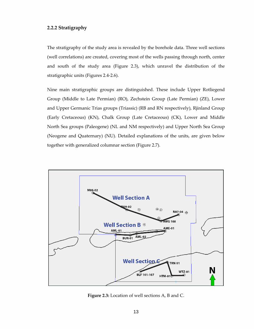
The stratigraphy of the study area is revealed by the borehole data. Three well sections

(well correlations) are created, covering most of the wells passing through north, center

and south of the study area (Figure 2.3), which unravel the distribution of the

stratigraphic units (Figures 2.4-2.6).

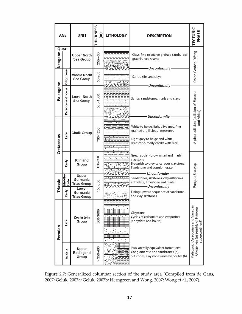
Nine main stratigraphic groups are distinguished. These include Upper Rotliegend

Group (Middle to Late Permian) (RO), Zechstein Group (Late Permian) (ZE), Lower

and Upper Germanic Trias groups (Triassic) (RB and RN respectively), Rjinland Group

(Early Cretaceous) (KN), Chalk Group (Late Cretaceous) (CK), Lower and Middle

North Sea groups (Paleogene) (NL and NM respectively) and Upper North Sea Group

(Neogene and Quaternary) (NU). Detailed explanations of the units, are given below

together with generalized columnar section (Figure 2.7).

Figure 2.3: Location of well sections A, B and C.

14

Figure 2.4: Well section A (see Figure 2.3 for its location).

15

Figure 2.5: Well section B (see Figure 2.3 for its location).

16

Figure 2.6: Well section C (see Figure 2.3 for its location).

17

Figure 2.7: Generalized columnar section of the study area (Compiled from de Gans,

2007; Geluk, 2007a; Geluk, 2007b; Herngreen and Wong, 2007; Wong et al., 2007).

18

2.2.2.1 Upper Rotliegend Group (RO) (Middle to Late Permian)

The Upper Rotliegend Group is the lowermost stratigraphic unit interpreted in the

seismic sections. It includes Slochteren and Silverpit Formations which are lateral

equivalents of each other (Geluk, 2007a) (Figure 2.8). According to borhole data, both

Slochteren and Silverpit formations subcrop in the study area since it is located at the

transition zone of these formations where they interfinger each other. Slochteren

Formation has fluvial and eolian origin and is composed of conglomerates and

sandstones, whereas Silverpit Formation, occur at the north relative to the Slochteren

Formation, was deposited in playa lake environment and composed of siltstones,

claystones and evaporates (Geluk, 2007a).

Figure 2.8: Generalized Permian and Triassic lithostratigraphy in the Netherlands

(adopted from Geluk, 2007b; Herngreen & Wong, 2007; Wong et al, 2007).

19

Due to its deep burial, some of the wells did not reach to the Upper Rotliegend Group

and the ones that reach did not fully penetrate it. The maximum observable thickness of

Upper Rotliegend Group is about 350-400 meters.

2.2.2.2 Zechstein Group (ZE) (Late Permian)

Zechstein Group comprises the upper Permian deposits. It overlies Upper Rotliegend

Group conformably. It is composed of six formations, namely Z1, Z2, Z3, Z4, Z5 and

Zechstein Upper Claystone Formation (Figure 2.8). Formations of Z1 to Z5 are

evaporitic cycles made up of carbonate, anhydrite and salt layers, covered by red and

grey anhydritic claystones of Zechstein Upper Claystone Formation (Van Adrichem

Boogaert & Kouwe, 1994 cited in Geluk, 2007).

Extensive halokinesis of Zechstein salt (mainly Z2 salt) results in highly variable

thickness distribution throughout the study area. The thickness of the Zechstein Group

varies from 300 meters to more than 2000 meters in places. Well top correlations reveal

a significant increase in thickness towards the center of the study area. Its greatest

thickness is observed in the TRN-01 well and reaches approximately 3000 meters

(Figure 2.4-2.6)

2.2.2.3 Lower and Upper Germanic Trias Groups (RB) (Triassic)

Lower Germanic Trias Group refers to Triassic deposits of Lower Buntsandstein,

Volpriehausen, Detfurth and Hardegsen formations (Van Adrichem Boogaert &

Kouwe, 1994). It overlies Zechstein Group conformably. Lower Buntsandstein

Formation consists of fine grained lacustrine sandstones and clay-siltstones.

Volpriehausen, Detfurth and Hardegsen formations consist of fining upward sequences

of sandstones and clay-siltstones (Geluk, 2007b).

The Upper Germanic Trias Group unconformably overlies Lower Germanic Trias

Group (Ziegler, 1990; Geluk & Röhling, 1997, 1999; Geluk, 2005). The Upper Germanic

20

Trias Group includes Solling, Röt, Muschelkalk, and Keuper formations (Van Adrichem

Boogaert & Kouwe, 1994) (Figure 2.8). The Solling Formation is composed of

sandstones overlain by fine-grained deposits, mainly siltstones and claystones. The Röt

Formation has a lower evaporitic part overlain by clay and siltstone dominated Upper

Röt Claystone Member. The Muschelkalk Formation show alternation of limestones

and marls at the lower and upper parts whereas middle part show an evaporitic origin,

consisting of halite, anhydrite and dolomites. The Keuper Formation is composed of

reddish and dark-coloured claystones alternating with thin layers of dolomite, fine-

grained sandstone and coal (Geluk, 2007b).

Triassic units are either absent or too thin, having a restricted areal distribution

throughout the study area. Well-tops correlation charts reveal that the Triassic Groups

have their maximum thickness at the center of the study area, gradually thinning

towards the locations with thick Zechstein deposits (Figures 2.4-2.6). The Lower

Germanic Trias Group reaches a maximum thickness of 300 meters and generally is

around 100-150 meters whereas Upper Germanic Trias Group is almost completely

absent, occur locally on the wells in the south (BLF-107, WTZ-01), and at the center

(AML-02, BUR-01) (Figure 1.). AML-02 Well shows the maximum thickness of the RN

which is approximately 370 meters. Well data of AML-02 reveals the presence Solling,

Röt and lower parts of the Muschelkalk Formation. Wells to the south shows a

complete absence of Muschelkalk and Keuper formations.

2.2.2.4 Rjinland Group (KN) (Early Cretaceous)

The Lower Cretaceous Rjinland Group unconformably overlies Upper and Lower

Germanic Trias groups and locally Zechstein Group where Triassic units area absent

(Figures 2.4-2.6). It is composed of Vlieland Sandstone, Vlieland Claystone and Holland

formations (Figure 2.9). The Vlieland Sandstone comprises shallow-marine sandstones

and local conglomeratic beds. Vlieland Claystone Formation consists of brownish grey

to grey calcareous claystones. Holland Formation is composed of grey and reddish

21

brown marls and marly claystones. At its lower part, thick incursions of greensands

and thin intercalations of bituminous shales occur (Herngreen & Wong, 2007).

Rjinland Group deposits vary in thickness from as low as 100 meters (where Zechstein

Group has its maximum thickness) to more than 300 meters.

Figure 2.9: Generalized post-Jurassic lithostratigraphical units of the Netherlands

(modified from Geluk, 2007b).

22

2.2.2.5 Chalk Group (CK) (Late Cretaceous – Early Paleocene)

The Chalk Group is a succession of marine limestones deposited during Cretaceous

(ranging from Cenomanian to Danian), resting conformably on Rjinland Group. It

consists of Texel, Ommelanden and Ekofisk formations (Figure 2.9). Texel Formation is

composed of light-grey to beige and white limestones and marly chalks together with

marl intercalations. Ommelanden Formation consists of white to grey, fine, argillaceous

limestones. The Ekofisk Formation is a succession of white, chalky limestones with rare

nodular and bedded flint layers and thin grey to green clay laminae (Herngreen &

Wong, 2007).

The Chalk group has a thickness of 700-1200 meters in most of the study area, however

in TRN-01 Well, where the Zechstein Group is thick, it has approximately 200 meters of

thickness. Well data shows that Ekofisk Formation is absent in the study area.

2.2.2.6 North Sea Supergroup (NS) (Tertiary - Recent)

Tertiary and Quaternary deposits are grouped together as the North Sea Supergroup,

overlying the Chalk Group unconformably (Wong et al., 2007). It is divided into Lower,

Middle and Upper North Sea groups (Figure 2.9).

The Lower North Sea Group, is a succession of sandstones, marls and clays. It consists

of Landen and Dongen formations, deposited in Paleocene to Eocene. Resting

unconformably over Lower North Sea Group, the Middle North Sea Group mainly

consists of sands, silts and clays. It is divided into Rupel and Veldhoven formations,

deposited during Oligocene. The Neogene and Quaternary deposits form the Upper

North Sea Group, and unconformably overlies Middle North Sea Group. It consists of

clays, fine to coarse grained sand and gravels (Breda and Oosterhout formations) and

Quaternary alluvium deposits (Wong et al., 2007).

23

CHAPTER 3

SEISMIC INTERPRETATION AND MODELING

3.1 Modeling Concept and Workflow

The purpose of 3D modeling is to create an ideal structural and stratigraphical model of

the subsurface in depth domain (solid earth model) by using seismic reflection (time

domain), borehole, velocity, and literature data.

The modeling process is divided into three phases. First part is the input of the

geological elements, namely, horizons and faults which are picked on seismic sections

with the aid of literature and borehole information. Picked horizons are then converted

to surfaces using appropriate interpolation techniques that produce unfaulted

structural framework. Similarly, faults are interpreted on seismic sections mainly by

utilizing horizon and seismic layer terminations. Second part of the procedure includes

the structural modeling that includes fault modeling, pillar gridding and generation of

faulted horizons, sequentially. This implies that first the model domain is gridded, then

inputs are edited, and finally faulted structural framework (static solid model) of the

subsurface is created. Since, all these procedures are performed in time domain (two-

way-travel time of seismic data), the final step in structural modeling involves depth

conversion of the model by defining several velocity models based on available velocity

information and conversion routines. In the following section, detailed information for

each step is given as illustrated in Figure 3.1.

24

Figure 3.1: Flowchart of the modeling process.

25

3.2 Seismic Interpretation

3.2.1 Defining and Picking the Key Horizons

Prior to seismic interpretation, the seismic data needs to be tied to well data in order to

correlate the horizons with the stratigraphy and to select the key horizons to be picked

and interpreted. The selection of horizons is performed by considering two criteria:

First criterion is the availability of the velocity data in order to make a proper depth

conversion at the end of the modeling process. Second criterion is the appraisal of the

seismic characteristics of horizons throughout the survey area. The candidate horizons

are correlated with the well (borehole) data by integrating the wells to seismic via

conversion of the well tops into time domain.

Based on the boreholes in and around the study area, the interval velocities of the

stratigraphic units comprising Rotliegend Group (RO), Zechstein Group (ZE), Lower

(RN) and Upper (RB) Germanic Trias Group’s, Rjinland Group (KN), Chalk Group

(CK), and North Sea Supergroup (NS) are obtained from company reports (discussed

later). For the simplicity and rapid lateral thickness variations Upper and Lower

Germanic Trias groups (RB and RN) are combined as a single unit (unit T) since they

are either absent or too thin, occurring in a restricted areal distribution in the study

area. Well data show that the occurrence of RB is much more common than RN so that

the interval velocity of RB is used for the combined unit (Unit T). By using the interval

velocities, the well data is converted into time domain. The distributions of the

boundaries of the stratigraphic intervals are then tied to the seismic sections. For

correlation, seismic profiles that do not show strong deformation patterns are chosen in

order to reduce the inaccuracy of time conversion with average interval velocities. Due

to the inaccuracy of time conversion, borehole deviation information, and off-set

between well location and seismic section, a perfect match between well-tops and the

startigraphical horizon boundaries can not be established previously, thus, the well-to-

seismic correlation can not be done directly at the locations where the inaccuracy

26

increases (mainly at the northern part of the study area). However distinct geological

changes on the unit boundaries (mainly the units above the ZE) are imprinted on the

seismic sections based on seismic facies and lateral amplitude variations such as

sharpness, presence of high and low amplitudes, positive and negative reflections

which can be traced throughout the survey area etc. Furthermore, a thickness

correlation was utilized between wells and seismic sections where strong shifts are

observed, in which group thicknesses are tried to be matched with reflections on

seismic sections (Figure 3.2)

Picking of the groups above the ZE is straightforward since they give region-wide

traceable high amplitude reflections. However, Zechstein salt layers give chaotic to

nearly transparent reflections as expected. However, the contained anydrite layers

towards the top of the Zechstein Group are very prominent in the seismic sections as

having very high amplitude values within semi transparent salt and fine-grained

matrix (Figure 3.3). On the other hand, the other lithologies within the ZE are difficult

to trace and only the layers of carbonate and fine grained clastics, which show parallel

reflections at the top of the salt boundary are distinguishable. In fact, the Zechstein

Group boundary can be also taken as the salt boundary (i.e. top of the transparent

layers), since those layers are too thin, in places.

Figure 3.2: Well seismic correlation depicted on a seismic line passing through 6 wells. Units NU, NM, NL, CK, KN, T and ZE can be

matched with well data (either directly or by matching thicknesses and observing shifts. Note, that there are slight mismatches

between well tops and horizons below Cretaceous (KN). This is due to local interval velocity variations).

27

28

Figure 3.3: Close-up view of the anhydrite, clay and carbonate layers within the

Zechstein Group.

After detailed examination of the seismic sections, five more interfaces are picked in

order to reveal the structural configuration, (salt-induced structures, namely folds and

faults) belonging to Cenozoic NS Supergroup. These units also display traceable

reflections. Two of these interfaces can be correlated with the well data, corresponding

to boundaries between Lower North Sea Group (NL) - Middle North Sea Group (NM)

and Middle North Sea Group - Upper North Sea Group (NU). Two more interfaces are

selected from NL and one from NU. Delineated stratigraphic units by these interfaces

are named as Lower North Sea Unit 1 (NL-1), Lower North Sea Unit 2 (NL-2), Lower

North Sea Unit 3 (NL-3), Upper North Sea Unit 1 (NU-1) and Upper North Sea Unit 2

(NU-2) (Figure 3.3).

As a result, 11 main seismic stratigraphic units were recognized and their interfaces

corresponding to their boundaries are picked as depicted in Table 3.1.

29

Table 3.1: Recognized stratigraphic units and corresponding picked horizons.

In general every 10th in- and cross-lines which corresponds to 250m*250m spacing were

interpreted from 3D surveys. For undeformed areas this interval is increased to 20. For

structurally complex regions, every in- and cross-line were studied in detail and related

horizons are picked at very fine intervals (25*25 m grid spacing) when necessary. These

correspond mainly to the top parts of the salt structure.

3.2.2 Surface Generation

Surfaces are the unfaulted representation of boundaries between seismic stratigraphic

units. They are created from interpreted horizon picks (in time domain) in order to

visualize the subsurface topography of each horizon (Figure 3.4). In this study, the

surfaces were created using “convergent interpolation algorithm” which converges

upon the solution iteratively adding more and more resolution with each iteration. This

means that general trends are retained in areas with little data while detail is honored

in areas where the data exist. Then each surface was visually examined for unwanted

30

surface anomalies due to misinterpretations. The observed anomalies were corrected

wherever encountered, then used for further analyses.

Figure 3.4: Picked horizons (left) are converted to surfaces in time domain (middle)

where surface attributes enable tracing of the faults (black lines). Then seismic lines

nearly perpendicular to the trends of the faults (right) are used for accurate

interpretation.

3.2.3 Fault Interpretation

The faults are detected by means of reflection offsets in seismic sections and the

morphological expressions i.e. high reliefs, sudden changes in slope etc. on the time

surfaces (Figure 3.4). Major faults in seismic scale, are chosen by utilizing bed

terminations from seismic sections and then traced by using time structure maps or 3D

surfaces which reveal the orientation of the fault throughout the area. As the

orientation of a fault is revealed, a seismic section is created in a direction that intersects

the fault at high angles in order to enable a reliable 3D interpretation of the fault. A

total number of 83 faults and fault segments were digitized in the study area (Figure

3.5).

31

Figure 3.5: Distribution of the interpreted faults (compare with Figure 3.7)

3.3 Structural Modeling

Structural modeling is a process by which the continuous surfaces are intersected by

the interpreted faults. This results in generation of faulted surfaces and optimum

representation of volumes and geometries of the stratigraphical units. The process

consists of three sub stages; fault modeling, pillar gridding and horizon generation

3.3.1 Fault Modeling

At this stage, the faults that were interpreted on the seismic sections are defined as

active faults in order to form the basis of the 3D grid in fault modeling stage. The model

was simplified in order to get rid of artifacts that may arise during the trimming of

surfaces, by combining the faults that are close to each other and truncating the

crossing faults. Faults that are too close to each other or too short (mainly antithetic and

synthetic faults of main fault system and radial faults) were eliminated. Out of 83 faults

interpreted in the area, 20 of them were chosen to be eligible for the modeling process.

32

3.3.2 Pillar Gridding

Pillar gridding stage involves generation of 3D grid skeleton of the structural model.

After defining the grid boundary, grids are assigned for the model area with a grid

interval of 200 meters (Figure 3.6). In order to facilitate the coordination between the

faults and the grids, “I” and “J” directions (mainly corresponding to N-S and E-W

directions respectively) were assigned to the faults by which the grid geometry was

shifted near the faults, depending on the fault geometry. This process is repeated until

acceptable grid geometry and even grid distribution is obtained. Pillar gridding stage is

finalized when three skeleton grids for top, mid and base of the model is created

(Figure 3.7).

Figure 3.6: Map view of the faults that are chosen for fault modeling process in which

crossing faults are truncated (shown by arrows) and minor faults which are

insignificant for modeling process are eliminated.

N

33

Figure 3.7: 3D view of top, middle and base grids with faults.

3.3.3 Generation of Faulted Horizons

The faulted structural framework is built in the making horizons stage where the faults

cut the selected surfaces so that the displacements are unraveled. The resulting surfaces

and faults form the 3D model in time domain.

In order to interpolate the stratigraphic relationships between layers correctly, “horizon

type” parameters are defined. This involves assigning type of the horizon. For example,

the boundaries between Germanic Trias Supergroup (T) and Rijnland Group (KN) and

Middle North Sea Group (NM) and Upper North Sea Group (NU-1) are unconformable

surfaces and thus chosen as “erosional”. Base ZE was chosen as “base” and the rest of

the interfaces are “conformable”.

Since all the faults were extended to the top and bottom surfaces of the model for

interpolation purposes, they should be assigned as “active” or “inactive” for each layer

in order to avoid unwanted displacements. For instance, as the Permian faults were

extended to the top surface (Upper North Sea Unit 2), the faults should be assigned as

“inactive” above the Permian interfaces (Triassic to Quaternary). Likewise as the

N

34

Cenozoic faults were extended to the bottom surface (base Zechstein), they should be

assigned as “inactive” below the Cenozoic interfaces.

The surfaces that are used in this step are the interpolated data of the horizon picks,

which means that the algorithm ignores the fault displacement along the fault surfaces

and forms continuous surface without a break. This results in drags along the faults

depending on the heave of the fault. During the implementation of displacement, this

will result in wrong fault displacements, if the surface and the faults were not properly

adjusted. To overcome this problem, “distance to fault” parameter was employed. It is

used to define the distance to the fault, where the interpolation algorithm ignores the

input data within this distance (buffer zone), increasing the quality of the resulting

model. Different distance values are chosen for each fault and also for each side of a

single fault. Results were manually examined and cross-correlated with the original

seismic data until getting the original fault displacements (Figure 3.8).

Figure 3.8: Change of the displacement amount depending on the distance to fault

parameter. In this case small distance parameter (a) result in erroneous fault

displacement due to smearing (b,c) whereas a larger displacement parameter (d) result

in more accurate fault displacement (e,f).

35

3.4 Velocity Models and Depth Conversion

Depth conversion is a crucial step in earth scientific modeling in order to recreate the

real geometry of the subsurface using computer algorithms. It corrects the geometry

and orientation of faults and horizons that is resulted from time domain and reveals the

true thicknesses of the stratigraphic layers and fault displacements. Furthermore, pull-

up, pull-down errors caused by variation of interval velocity as in the case of salt

structures, which have rapid lateral velocity variations, are corrected so that the true

geometries of the layers and structures can be revealed.

In order to accomplish correct time-to-depth conversion, different velocity models were

tried and the best suited one was selected for the model. Parameters for each velocity

model were obtained from van Dalfsen et al. (2006) as part of the VELMOD project of

Scientific and Technological Organization of the Netherlands (TNO), in which a seismic

velocity distribution map was prepared for the entire Netherlands region, both onshore

and offshore, based on instantaneous sonic velocities. The parameters in the report

were subdivided into regions and the ones that fall in the study area were selected.

The applied depth conversion techniques are discussed below.

3.4.1 Constant (Interval) Velocity Model

Interval velocity model uses constant velocity value (V=Vint) at each location for a given

stratigraphic interval (in this case, stratigraphic group). For the Germanic Trias

Supergroup (T) (which includes Lower and Upper Germanic Trias groups), the velocity

value of Lower Germanic Trias Group was used since Upper Germanic Trias Group can

be neglected due to its absence in places, and its negligible thickness wherever present

throughout the study area. Interval velocities that are used were depicted in Table 3.2.

36

3.4.2 Vok Method

Vok method utilizes velocity changes in the vertical direction at each XY in a particular

stratigraphic interval. The method has the relationship V=Vo+kZ where Vo represents the

velocity at datum, k is the factor of change in the velocity and Z is the distance of the

point from datum (Table 3.2) i.e. depth in meters. The values of Vo and k are obtained

from linear regression of velocity data obtained from different wells in the region. As

for the interval velocity model, RN values are also neglected in this model and

parameters of RB were used for unit T. Only the salt layer (ZE) has a constant value

rather than having the Vo and k parameters in this model since salt is not affected by

compaction (depth independent) and needs to be treated differently than other layers.

Table 3.2: Parameters of velocity models for each stratigraphic unit.

Int. Veloc. Model Vok Method

Group Name Vint (m/s) Vo (m/s) k

NS 1981.3 1775 0.288

CK 3784.3 2200 0.882

KN 3053.3 2000 0.492

T (RB) 3671 2800 0.362

ZE 4700.4 4500 0

3.4.3 Assessment of the Velocity Models

Depth conversions from both velocity models gave similar results, down to the top

Chalk (CK) layer. Resulting depth values are nearly coincident at the layers closer to the

surface (Figure 3.9). Vok method gives slightly better results down to Top CK surface

where a consistent shift is observed in the interval velocity model. This shift is more

37

prominent in northern parts of the study area. The higher difference between two depth

conversion methods occur at the Top KN and lower horizons, in which the Vok method

is superior to interval velocity model if not perfect. The inaccuracy of the interval

velocity model arises from the thickness of the units. The unit CK has higher thickness

and also very rapid facies changes (Herngreen & Wong, 2007) compared to all the units

above, which are more or less matching with the well tops. Further incorrect constant

velocity value for CK simply multiplies the error, resulting in inaccurate depth value

for base CK (top KN). Due to this inaccuracy, interfaces below top KN (top T, top ZE)

are shifted from the well top locations. Largest error occurs at the Base ZE due to high

thickness of unit ZE, as in the case of CK, and its high velocity value. As the error from

the layers above is added consequently to the layers below, the inaccuracy is gradually

getting larger (Figure 3.9).

The accuracy of the velocity model is tested by manual well top-surface correlation in

depth domain. After careful assessment of the depth models, especially by checking

their match with the well tops, the Vok method found to be more suitable for further

analyses. A final correction is applied to the Vok model in which the depth model is

corrected at the well locations using the depth information of well tops (the velocity

values are recalculated at each well site in order to match the surfaces to the

corresponding well tops.

The well data correction is applied after the selection of the velocity model since

executing the well correction prior to the model selection will prevent the appraisal of

velocity models (Figure 3.9).

Figure 3.9: Correlation of depth converted surfaces with the well tops. Same cross section, passing through 4 wells are used for cross-

correlation of velocity models. The mismatch error is higher in interval velocity model (a) compared to Vok method which gives

nearly perfect results with slight shifts (b) which is corrected with the well tops (c).

38

39

CHAPTER 4

RESULTS

4.1 Model Outputs

The produced depth model comprises 20 faults representing the structural grain and 10

seismic stratigraphic units (Figure 4.1). These include Permian Zechstein Group (ZE),

Germanic Trias Supergroup (T), Lower Cretaceous Rjinland Group (KN), Late

Cretaceous Chalk Group (CK), 3 subunits of Lower North Sea Group (NL1, NL2, NL3),

Middle North Sea Group (NM), and Upper North Sea Group (NU) (Figure 4.1). The

isopach (Figure 4.2) and sub-surface maps, interpreted seismic sections (Figures 4.3 &

4.4) and cross sections are used to discuss the state-of-the art of the structure and

stratigraphy of the study area.

Figure 4.1: Vertically (x4) exaggerated perspective view (a) and map view (b) of the

model with layers, faults and position of the used wells.

40

Figure 4.2: Isopach maps of the seismic stratigraphic units. White areas are zero

thickess zones. (D: depleted, E: eroded. Unmarked areas are the barren zones due to

faulting). See Appendix A for higher resolution of these figures.

41

Figure 4.2: (Continued.)

Figure 4.3: Interpreted and vertically (x5) exaggerated composite (arbitrary) seismic section in time domain.

42

Figure 4.4: Stratigraphic and structural interpretation of the composite seismic section on Figure 4.3, showing major seismic

stratigprahic units, faults and unconformities. Section is cutting across the main salt cored anticline (left) and dome shaped salt

pillow (right).

43

44

4.2 Characteristics of Seismic-Stratigraphic Units

4.2.1 Permian: Zechstein Group

Only the top of the Permian Rotliegend Group is picked during seismic interpretation,

which also constitutes the base of the 3D model and the Zechstein Group. The isopach

map of Zechstein Group indicates 3 different thickness zones; (i) Thick zones where salt

movement took place, generally around 1500 to 2000 meters, locally reaching up to 2700

meters mainly at the southeastern part of the study area, (ii) moderate thickness zones

in undeformed regions are ranging from 500 to 1000 meters, and (iii) lowest thicknesses

occur, mainly at the western flank of the main salt structure (Figure 4.2). The Zechstein

Group generally shows a conformable relationship with Upper Permian Rotliegend

Group at the bottom. However due to the extensive salt movement, the contact is

disturbed at many localities (Figure 4.4).

4.2.2 Triassic: Germanic Trias Supergroup

Germanic Trias Supergroup which is Triassic in age, is bounded by Permian Zechstein

Group at the bottom and erosional base of Lower Cretaceous Rjinland Group at the top.

The unit comprises Lower and Upper Germanic Trias groups. Triassic units are

relatively thin probably due to erosion and/or nondeposition. The erosional phase is

evidenced by the angular unconformity between Triassic and Cretaceous units.

However the angular relationship disappears through out most areas of the study area

and the conformable appearance of Triassic and Cretaceous units complicates the

recognition of the unconformity (Figure 4.4). Its difficult to identify from the reflection

characteristics, however borehole data reveals a clear absence of Upper Germanic Trias

Group nearly throughout all of the survey area, except that it locally exist at the

western flank of the main salt structure where the whole Triassic unit reaches its

maximum thickness which is around 700 meters. This area was probably a mini basin

45

under the control of the salt movement. A clear onlap relationship is not observed

between Triassic units and Permian Zechstein, and the lower parts of the Triassic layers

show a conformable relationship with the Zechstein unit (Figure 4.4). It is important to

note that the group is completely absent at the northwestern and southwestern part of

the study area. In general, in the rest of the area the Lower Germanic Trias Group has

100-300 meters of thickness and only reaches 400 meters at the eastern parts of the

study area (Figure 4.2).

4.2.3 Cretaceous: Rjinland and Chalk Groups

Rjinland and Chalk groups are conformable units of Cretaceous, resting above a Base

Cretaceous Unconformity and below Lower North Sea Group. Rjinland Group has a

consistent thickness distribution ranging between 200 and 250 meters (Figures 4.4 and

4.10). Chalk group is relatively thicker compared to other units and reaches up to 750 to

1000 meters (Figures 4.2 and 4.4) throughout the study area.

4.2.4 Cenozoic: North Sea Supergroup

The Cenozoic sequence above the Cretaceous Chalk Group comprises the North Sea

Supergroup which is divided into three subgroups as Lower, Middle and Upper North

Sea groups. The Lower North Sea Group is further divided into three sub units, coded

as NL1, NL2 and NL3 and have a total thickness of 500-600 meters. Middle North Sea

Group is relatively thin having 50-100 meters of thickness, locally reaching up to 300

meters at the southeastern part of the study area (Figures 4.2). A major angular

unconformity is detected between Middle and Upper North Sea groups (Early Miocene

Unconformity). Both the Lower and the Middle North Sea groups were subjected to

erosion (Figure 4.4). Upper North Sea Group consists of Neogene and Quaternary

deposits, having around 200 meters of thickness (Figure 4.2).

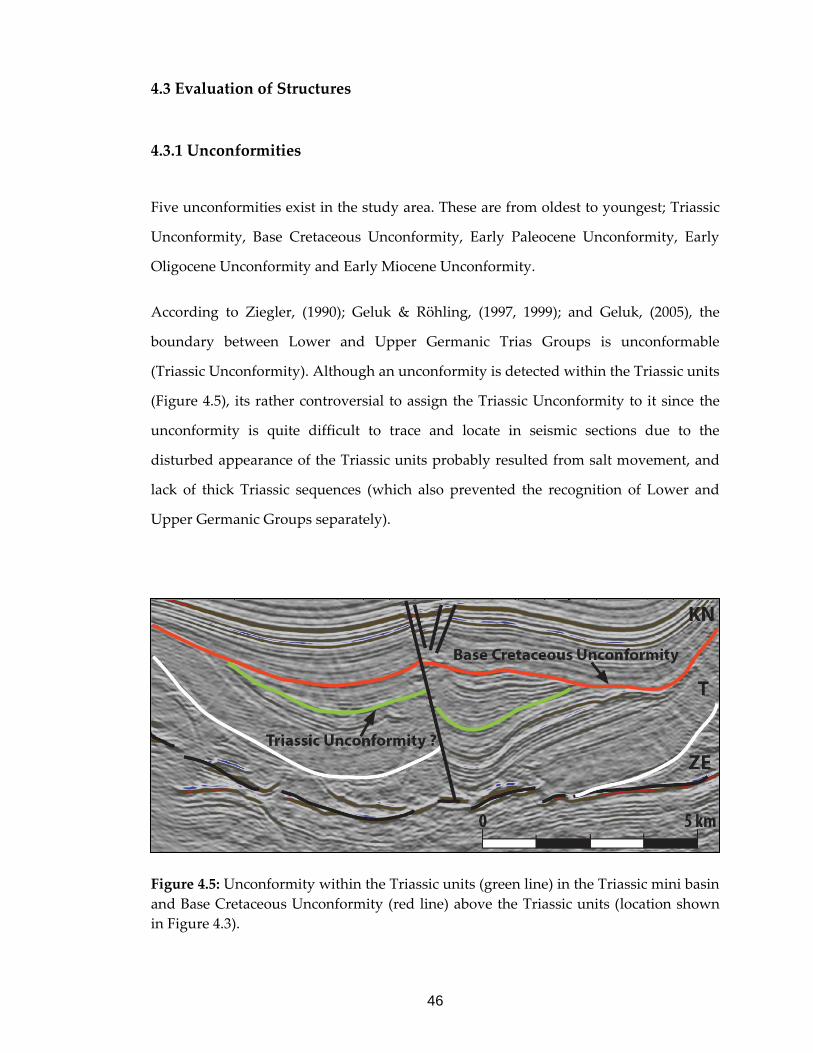
46

4.3 Evaluation of Structures

4.3.1 Unconformities

Five unconformities exist in the study area. These are from oldest to youngest; Triassic

Unconformity, Base Cretaceous Unconformity, Early Paleocene Unconformity, Early

Oligocene Unconformity and Early Miocene Unconformity.

According to Ziegler, (1990); Geluk & Röhling, (1997, 1999); and Geluk, (2005), the

boundary between Lower and Upper Germanic Trias Groups is unconformable

(Triassic Unconformity). Although an unconformity is detected within the Triassic units

(Figure 4.5), its rather controversial to assign the Triassic Unconformity to it since the

unconformity is quite difficult to trace and locate in seismic sections due to the

disturbed appearance of the Triassic units probably resulted from salt movement, and

lack of thick Triassic sequences (which also prevented the recognition of Lower and

Upper Germanic Groups separately).

Figure 4.5: Unconformity within the Triassic units (green line) in the Triassic mini basin

and Base Cretaceous Unconformity (red line) above the Triassic units (location shown

in Figure 4.3).

47

Base Cretaceous Unconformity is mostly observed between Triassic Germanic

Supergroup and Cretaceous Rjinland Group (Figures 4.4 & 4.5). Most of the Germanic

Trias Supergroup was eroded, especially Upper Germanic Trias Group which is nearly

absent throughout the study area. The unconformity is effective on the crest of the salt

structures where Triassic units are completely eroded. The Base Cretaceous

Unconformity is an angular unconformity where the angular relationship between the

units is most prominent at the crest and flanks of the salt structures. Gradual

disappearance of the angular relationship away from the salt structures and the

complete absence of Jurassic units in the study area favor the possibility that the

Jurassic units are not deposited rather than being eroded.

Early Paleocene Unconformity which exists between Cretaceous Chalk Group and

Paleocene-Eocene Lower North Sea Group and Early Oligocene Unconformity that

exists between Lower North Sea Group and Oligocene Middle North Sea Group are

based on literature and could not be determined from the seismic sections due to lack of

angular relationship between the units (Figure 4.4), and existence of all of the

formations that make up the groups in the well data.

Therefore, it is inferred that the units involved within this unconformity are below the

limits of seismic resolution (ca. 50m) or it is a disconformity and the units below and

above the unconformity are parallel to each other within the study area.

The Early Miocene Unconformity is an angular unconformity observed between

overlying Upper North Sea Group and underlying Oligocene Middle North Sea Group

and Eocene Lower North Sea Group. Erosion was effective mainly at the crest of the salt

structures and faulted areas where the Middle North Sea Group and most of the Lower

North Sea Group was eroded. (Figures 4.4 & 4.6).

48

Figure 4.6: Early Miocene Unconformity (yellow line) above the crest of the salt

structure. Erosion is effective near the faults and crest where Middle North Sea and

Lower North Sea groups are extensively eroded (location shown in Figure 4.3).

4.3.2 Salt Structures

Salt tectonics is the major structural characteristic of the study area. The Zechstein Salt

is extensively mobilized and ascent more than 2500 meters (Figure 4.7). It forms non-

piercing salt pillows throughout the study area.

The main salt structure dominating the structural grain and stratigraphic development

of the area is a N-S-elongated salt cored anticline (Figure 4.4). The anticline is

approximately 18 km long and 1.5 km wide. In the core of the anticline salt has reached

at a maximum of 2700 meters of thickness (Figure 4.2). The zero thickness zone at the

western flank of the main salt structure indicates a salt depletion (Figure 4.4). One of

the most prominent structure in the overlying units of Zechstein Group is presence of

rim synclines within the Triassic units. As mentioned previously, contrary to

unconformable upper levels of Triassic units, they are conformable at the lower levels

49

(Figures 4.4 and 4.5). The Rjinland Group, Chalk Group and North Sea Supergroup are

the folded units of the salt cored anticline (Figure 4.4). Although they do not display

any rim-syncline development, they are intersected by salt-related faults. Furthermore,

the true thickness of these units is significantly thicker away from the limbs and the

crest of the fold.

In addition to this, at the northeastern part of the salt cored anticline, a dome-shaped

salt pillow is also present. It has a wavelength of 6 km and the salt column has a vertical

thickness of 1800 meters. The central part of the dome is associated with relatively small

scale radial faults (Figure 4.4).

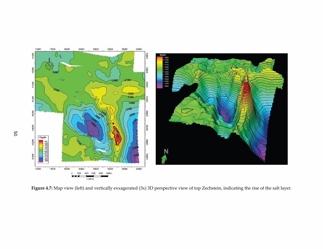
Figure 4.7: Map view (left) and vertically exxagerated (3x) 3D perspective view of top Zechstein, indicating the rise of the salt layer.

50

51

4.3.3 Faults

The study area is dominated by normal faults and formed in two different settings. The

basement faults formed before the deposition of the Zechstein Salt and displaced the

Rotliegend Group. Other faults are associated with the units above the Zechstein Salt

(overburden faults) and most of them are the salt-induced faults. These two sets of the

faults are not connected and are decoupled from each other by the Zechstein Salt.

The base Zechstein topography, associated with a couple of NW-SE oriented large scale

normal faults, acted as a primary control on the thickness of the overlying Permian

Zechstein salt and Triassic deposits (Figures 4.8 and 4.9). The depth model indicates

several N-S-and NW-SE-oriented structural depressions at the base of the Zechstein

Salt, possibly indicating a graben or half graben structure, aligned parallel to the salt

and salt induced structures (Figure 4.8). The possible graben and half-graben structures

are not observable before the depth conversion due to the pull-up anomalies beneath

the thick Zechstein Salt, hence the interpretations can be done only in final depth model

(without direct fault interpretations from seismic sections).

Units above the Zechstein salt are associated with several large-scale Cenozoic normal

faults possibly resulted from the salt tectonic deformation (Figure 4.10). Most

significant faults are the N-S-oriented normal growth faults, forming a convergent

conjugate transfer zone (Figures 4.10-4.12). Northern branch of the fault is dipping west

whereas the southern branch is dipping east. These two structures overlap at the crest

of the anticline where they result in a graben geometry, whereas they control half

grabens away from the crest. In other words, major faults associated with the transfer

zone have asymmetrical half-graben geometry away from the transfer zone and

symmetrical graben geometry with small scale synthetic and antithetic faults at the

center of the transfer zone.

Figure 4.8: Map view (left) and vertically exaggerated (x3) 3D perspective view (right) of Base Zechstein, showing Permian faults and

possible graben-half graben structures.

52

Figure 4.9: Cross section A-B-C, indicated on Figure 4.8. Manifestation of basement (red) and overburden faults (blue). Note that the

overburden faults do not penetrate below the Zechstein (ZE). Note also that only major faults are indicated.

53

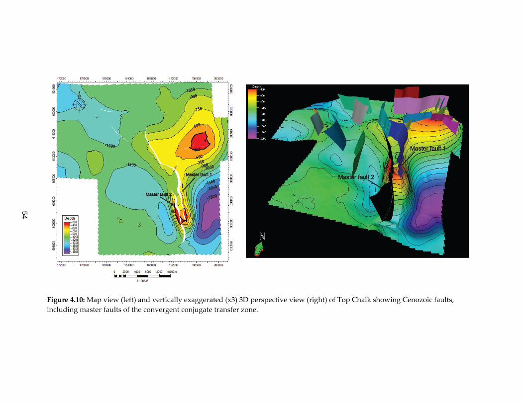
Figure 4.10: Map view (left) and vertically exaggerated (x3) 3D perspective view (right) of Top Chalk showing Cenozoic faults,

including master faults of the convergent conjugate transfer zone.

54

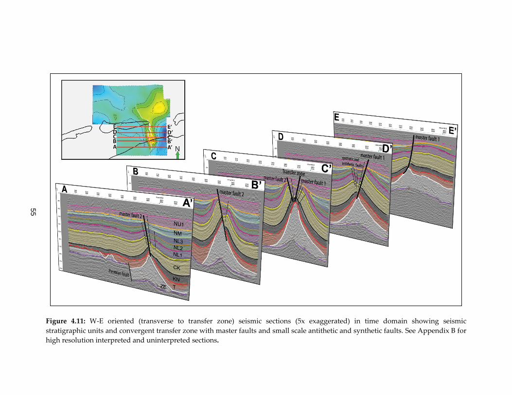
Figure 4.11: W-E oriented (transverse to transfer zone) seismic sections (5x exaggerated) in time domain showing seismic

stratigraphic units and convergent transfer zone with master faults and small scale antithetic and synthetic faults. See Appendix B for

high resolution interpreted and uninterpreted sections.

55

56

Figure 4.12: Model representation of convergent conjugate transfer zone, showing

barren zones of the master faults at each Cenozoic surface (top), and 3D perspective

view of the transfer zone above the salt layer with master faults and nearly

perpendicular cross sections (bottom).

57

CHAPTER 5

DISCUSSION AND CONCLUSIONS

5.1 Structural Development and Salt Tectonics

The study area experienced several phases of tectonic deformation since the Early

Paleozoic. However the complex tectonic history is reflected as a rather simple

structural grain in the area since it covers only small part of the deformed area.

The oldest studied deformation feature in the region is related to the Permian basement

faulting, as indicated by NW-SE Permian faults and graben, half-graben structures in

the model. This basement morphology during the deposition of the Zechstein Salt gave

way to the significant thickness variation of the salt and uneven deposition overlying

Triassic units.

The first salt movement was initiated in the Triassic, most probably during E-W

Mesozoic rifting i.e breaking up of Pangea. Initially deposited lower parts of the

Triassic units (Lower Germanic Trias Group) are conformable with the Permian

Zechstein Salt indicating that salt was not mobilized yet. As the salt movement was

initiated, the ascent of the salt created mini basins and rim synclines at flanks of the

diapirs into which Triassic units were continue to be deposited. Gradual decrease in the

dip of the Triassic beds and small-scale angular unconformities observed on the mini

basin evidence a synkinematic deformation during the salt movement.

The first salt movement is inferred to be driven by overburden pressure (differential

loading) and buoyancy forces. The locus of movement was towards the areas where the

58

salt was thickest such as N-S-oriented graben center (Figure 5.1). The thickness of the

salt plays an important role for the buoyancy forces to overcome the cohesion and

internal frictional angle of the salt. However buoyancy forces are not large enough to

overcome the overburden pressure due to the low strength of salt (Hudec & Jackson,

2007). In some parts of the study area, more than 600 meters thick Zechstein Salt is

stable and have not undergone into salt tectonism yet. Therefore, the salt movement

needs to be primarily driven by differential loading. Like the buoyancy forces,

differential loading is also active on the locations where basement faults cause uneven

sediment distribution over the Zechstein (Figure 5.1a). As a result, buoyancy forces and

differential loading must have acted coevally and drive the salt movement laterally and

vertically leading to salt tectonics in locations especially where large-scale basement

faults are present that controlled both the thickness and the depositional setting of the

salt and overlying sediments. As the salt structures grew, they followed the N-S trends

where the salt was thickest and were parallel to the underlying basement faults. The

salt movement was possibly promoted by Triassic E-W extension which was related to

break-up of Pangea.

During the Middle Jurassic uplift, the Friesland Platform was partly emerged and

sediment deposition restricted only to the mini basins (Figure 5.1b). Friesland Platform

was completely established during the Late Jurassic-Early Cretaceous events (Duin et

al., 2006) in which Jurassic and Triassic units were eroded. There is no evidence of

Jurassic deposition in the study area, although the areas around Friesland Platform

were site of deposition during the Jurassic (de Jager, 2007). There is a possibility that the

sedimentation might have taken place at least in the mini basins, however, they must

have been eroded completely during Late Jurassic-Early Cretaceous inversion events

(Cimmerian Orogeny). Locally the erosion has reached down to Permian Zechstein

levels.

Since the Lower Cretaceous Rinjland and Upper Cretaceous Chalk and lower parts of

the Cenozoic Lower North Sea groups have no sign of salt movement as implied by the

absence of synkinematic indicators related to salt movement, the first phase of salt

59

diapirism lasted prior to the deposition of Lower Cretaceous units. The cessation of salt

movement might be resulted from the termination of Late Jurassic deformation and

presence of tectonic quiescence period during the Cretaceous-Early Tertiary. This

resulted in deposition of thick Cretaceous units (Rjinland and Chalk groups) and lower

parts of the Lower North Sea Group above the salt during regional subsidence and

rising of sea levels (De Jager, 2007) (Figure 5.1c). These events must have brought

tectonic balance to the system.

There is no clear evidence related to Late Cretaceous - Early Tertiary Alpine Orogeny in

the region which was characterized by N-S compression. In other words, the inversion

related pop-up structures and uplift features are absent in the area. This implies that the

Alpine compression was not directly effective in the study area. However a second

phase of salt movement should have taken place during the deposition of upper Lower

North Sea Group (NL2 and NL3) and Middle North Sea Group in Eocene-Oligocene, in

which the prekinematic units; Rjinland Group, Chalk Group and Lower North Sea

Unit-1 are folded and eroded, and were forming the salt-cored anticline while the area

was under control of regional shortening and uplift, during the late pulses of Alpine

Orogeny. The second phase is evidenced by formation of N-S-oriented Cenozoic

normal growth faults (Figure 4.10) and local thinning of the Lower North Sea Group

units 2, 3 and Middle North Sea Group, towards the core of the salt anticline (Figure

5.1d).

As the uplift, salt movement and deposition continued contemporaneously (and

gradually diminished in time) the crest of the salt structures were subjected to erosion,

forming the Early Miocene Unconformity. The erosion is effective especially on the

footwall blocks of the growth faults at the crest of the salt-cored anticline where Middle

and most of the Lower North Sea Groups are eroded.

The Late Tertiary structural events (Rhine Graben rifting) lead to subsidence (den

Hartog Jager, 2007) and resuming of deposition also above the crest of salt structures

(Neogene Upper North Sea Group). Presence of the growth faults which penetrated the

60

Upper North Sea Group and to surface indicates that the salt movement has been

taking place recently (Figure 5.1e). Therefore, the salt movement and the faults at the

crest of the diapirs are active faults and there is seismic risk for the region.

It is important to note that the salt structures are associated with normal faulting both

at the basement and overburden. This implies that the faults mainly in the basement

provided space and relief and differential loading for the salt to nucleate and enhance

salt movement. On the other hand, the faults above the salt are followed to some extent

the same trend of the basement faults although, the basement and overburden faults

are not directly linked since the Zechstein salt acted as a detachment surface decoupling

the basement structures from overlying structural grain. This relationship is interpreted

as the control of the basement faults on the salt movement and development of salt

related structures (Figure 5.2).

In conclusion, although the thick Zechstein salt and its structures acted as a detachment

horizon, the structural grain of the basement is reflected on the overlying structural

grain.

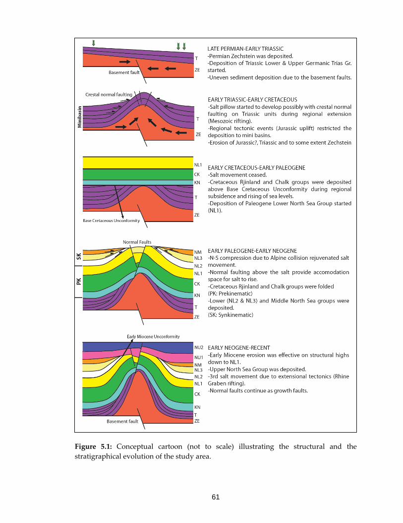
61

Figure 5.1: Conceptual cartoon (not to scale) illustrating the structural and the

stratigraphical evolution of the study area.

62

Figure 5.2: Top CK, Top ZE and Base ZE surfaces showing the coinciding orientation of

basement graben-half graben system, salt pillow and convergent conjugate transfer

zone.

5.2 Summary and Conclusions

Four main tectonic phases shaped the geology of the study area. These include

Paleozoic Caledonian and Variscan Orogeny (assembly of Pangea supercontinent),

Early Mesozoic rifting (break up of Pangea), Alpine inversion (collision of Europe and

Africa) during the Late Cretaceous to Early Tertiary, and Oligocene to recent

development of the Rhine Graben rift system. In this study, the effect and structures of

the last three tectonic phases are manifested. Together with these tectonic phases, the

Late Permian Zechstein Salt encountered mobilization and produced structures related

to those movements.

A computer based 3D solid model is constructed for the study area located within the

Friesland Platform by integrating 3D seismic and borehole data. The constructed model

revealed the structural and stratigraphic evolution of the area. Key horizons and major

faults were picked from seismic sections and interpreted. Well data was tied to the

63

seismic horizons in order to correlate and delineate the horizons. After the construction

of model in time domain, it was converted into depth domain in order to reveal the true

geometry of the subsurface.

The constructed model, includes 20 faults and 10 seismic stratigraphic units that

include Permian Zechstein Group (ZE), Triassic Germanic Trias Supergroup (T), Lower

Cretaceous Rjinland Group (KN), Late Cretaceous Chalk Group (CK), 3 subunits of

Lower North Sea Group (NL1, NL2, NL3), Middle North Sea Group (NM), and Upper

North Sea Group (NU). The model was used to create isopach and subsurface maps of

seismic stratigraphic units and to map out the faults, and to produce cross sections, 3D

perspective views of the subsurface.

The kinematic evolution of the Zechstein salt and the present structural grain of the

northern Friesland is the result of at least 3 phases of regional tectonic deformation that

shape the subsurface geology.

It is proposed that thickness variations of Zechstein Salt, possibly due to large-scale

basement faults, induced differential loading that acted as triggering mechanism for the

salt movements together with buoyancy forces, which also controlled the geometry and

orientation of the overlying structural grain. The salt structures are associated with a

convergent normal fault accommodation zone. In other words, the activity of these

faults in the overburden is related to salt movement which, in turn, provided space and

relief for the ascent of salt.

The graben-,half-graben system at the basement, salt structure and overlying

convergent transfer zone, are parallel and coinciding with N-S orientation. However

they are not linked since the Zechstein salt acts as a detachment horizon decoupling the

basement structures from the overlying structures.

64

REFERENCES

De Jager, J., 2003. Inverted basins in the Netherlands, similarities and differences.

Netherlands Journal of Geosciences / Geologie en Mijnbouw 82: 339–349.

De Jager, J., 2007. Geological Development. In: Wong, Th.E., Batjes, D.A.J. & De Jager, J.

(eds): Geology of the Netherlands. Royal Netherlands Academy of Arts and Sciences

(Amsterdam): pp. 5-26.

Duin, E.J.T., Doornenbal, J.C., Rijkers, R.H.B., Verbeek, J.W. & Wong, Th.E., 2006.

Subsurface structure of the Netherlands – results of recent onshore and offshore

mapping. Netherlands Journal of Geosciences / Geologie en Mijnbouw 85: 245–276.

De Gans, W., 2007. Quaternary. In: Wong, Th.E., Batjes, D.A.J. & De Jager, J. (eds):

Geology of the Netherlands. Royal Netherlands Academy of Arts and Sciences

(Amsterdam): pp. 173-195

Geluk, M. C., 2007a. Permian. In: Wong, Th.E., Batjes, D.A.J. & De Jager, J. (eds):

Geology of the Netherlands. Royal Netherlands Academy of Arts and Sciences

(Amsterdam): pp. 63-83.

Geluk, M. C., 2007b. Triassic. In: Wong, Th.E., Batjes, D.A.J. & De Jager, J. (eds):

Geology of the Netherlands. Royal Netherlands Academy of Arts and Sciences

(Amsterdam): pp. 85-106.

Herngreen, G.F.W., Kouwe, W.F.P. & Wong, Th.E., 2003. The Jurassic of the

Netherlands. In: Ineson, J.R. & Surlyk, F. (eds): The Jurassic of Denmark and Greenland.

Geological Survey of Denmark and Greenland Bulletin 1: 217–229.

65

Herngreen, G.F., Wong, Th.E., 2007. Cretaceous. In: Wong, Th.E., Batjes, D.A.J. & De

Jager, J. (eds): Geology of the Netherlands. Royal Netherlands Academy of Arts and

Sciences (Amsterdam): pp. 127-150.

Heybroek, P., 1975. On the structure of the Dutch part of the Central North Sea Graben.

In: Woodland, A.W. (ed.): Petroleum and the Continental Shelf of Northwest Europe.

Applied Science Publishers (Barking): 339–351.

Hudec, M. R., and Jackson, M. P. A., 2007, Terra infirma: understanding salt tectonics:

Earth-Science Reviews, v. 82, p. 1–24.

Pannekoek, A.J. (ed.), 1956. Geological history of the Netherlands– Explanation to the

general geological map of the Netherlandson the scale of 1 : 200 000. Staatsdrukkerij- en

uitgeverijbedrijf(’s-Gravenhage): 147 pp.

Pharaoh, P., England, R. & Lee, M., 1995. The concealed Caledonide basement of

eastern England and the southern North Sea – a review. Studia geoph. et geod. 39: 330–

346.

Remmelts, G., 1995. Fault-related salt tectonics in the southern North Sea, the

Netherlands. In: Jackson, M.P.A., Roberts, D.G. & Snelson, S. (eds): Salt tectonics: a

global perspective. American Association of Petroleum Geologists,Memoir 65: 261–272.

Remmelts, G., 1996. Salt tectonics in the southern North Sea, the Netherlands. In:

Rondeel, H.E., Batjes, D.A.J. & Nieuwenhuijs, W.H. (eds): Geology of gas and oil under

the Netherlands. Kluwer (Dordrecht): 143–158.

Van Adrichem Boogaert, H.A. & Kouwe, W.F.P. (compilers), 1993–1997. Stratigraphic

nomenclature of the Netherlands, revision and update by RGD and NOGEPA.

Mededelingen Rijks Geologische Dienst 50.

66

Van Buggenum J.M., den Hartog Jager D.G., 2007. Silesian. In: Wong, Th.E., Batjes,

D.A.J. & De Jager, J. (eds): Geology of the Netherlands. Royal Netherlands Academy of

Arts and Sciences (Amsterdam): pp. 43-62.

Van Dalfsten, W., Doornenbal, J.C., Dortland S., Gunnink, J.L., 2006. A comprehensive

seismic velocity model for the Netherlands based on lithostratigraphic layers.

Netherlands Journal of Geosciences / Geologie en Mijnbouw 73: 99–127.

Van Wees, J.D., Stephenson, R.A., Ziegler, P.A., Bayer, U., Mc-Cann, T., Dadlez, R.,

Gaupp, R., Narkiewicz, M., Bitzer, F. & Scheck, M., 2000. On the origin of the Southern

Permian Basin, Central Europe. Marine and Petroleum Geology 17: 43–59.

Wong, Th.E., de Lugt I.R., Kuhlmann G., Overeem I., 2007. Tertiary. In: Wong, Th.E.,

Batjes, D.A.J. & De Jager, J. (eds): Geology of the Netherlands. Royal Netherlands

Academy of Arts and Sciences (Amsterdam): pp. 151-171

Ziegler, P.A., 1988. Evolution of the Arctic-North Atlantic and the western Tethys.

American Asociation of Petroleum Geologists, Memoir 43, 198 pp, 30 plates.

Ziegler, P.A., 1990. Geological Atlas of Western and Central Europe, 2nd edition.

Geological Society Publishing House (Bath; distributors), 239 pp, 56 encl.

Ziegler, P.A., 1994. Cenozoic rift system of western and central Europe: an overview.

Geologie en Mijnbouw 73: 99–127.

67

APPENDIX A

ISOPACH MAPS OF THE SEISMIC STRATIGRAPHIC UNITS

Figure A.1: Isopach map of Zechstein Group. D: salt depleted areas.

68

Figure A.2: Isopach map of Germanic Trias Supergroup. E: eroded areas.

69

Figure A.3: Isopach map of Rjinland Group.

70

Figure A.4: Isopach map of Chalk Group.

71

Figure A.5: Isopach map of Lower North Sea Group. E: eroded areas.

72

Figure A.6: Isopach map of Middle North Sea Group. E: eroded areas.

73

Figure A.7: Isopach map of Upper North Sea Group.

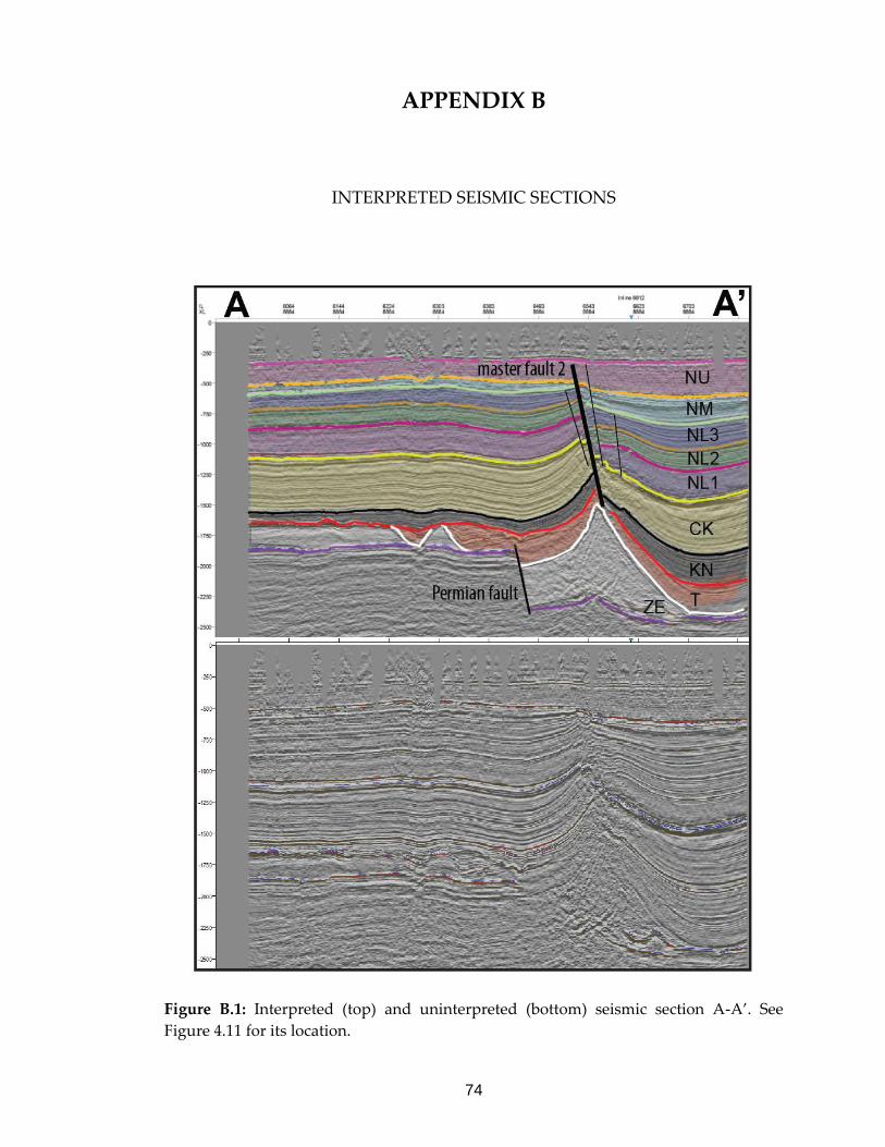
74

APPENDIX B

INTERPRETED SEISMIC SECTIONS

Figure B.1: Interpreted (top) and uninterpreted (bottom) seismic section A-A’. See

Figure 4.11 for its location.

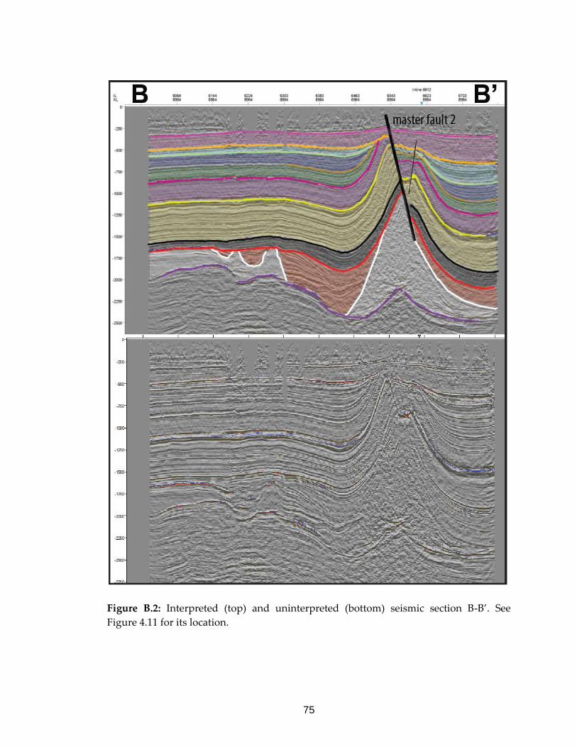
75

Figure B.2: Interpreted (top) and uninterpreted (bottom) seismic section B-B’. See

Figure 4.11 for its location.

76

Figure B.3: Interpreted (top) and uninterpreted (bottom) seismic section C-C’. See

Figure 4.11 for its location.

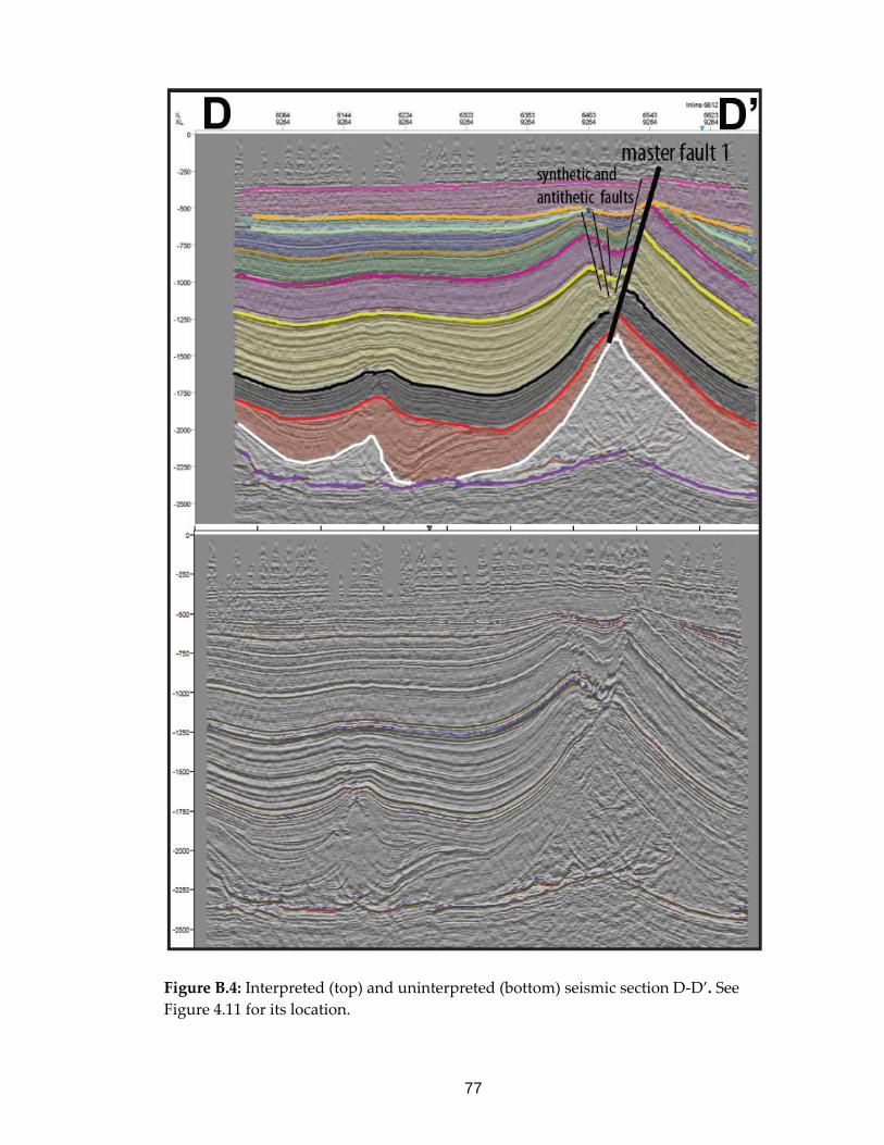
77

Figure B.4: Interpreted (top) and uninterpreted (bottom) seismic section D-D’. See

Figure 4.11 for its location.

78

Figure B.5: Interpreted (top) and uninterpreted (bottom) seismic section E-E’. See

Figure 4.11 for its location.