3D Seismic Forward Full-Wave Modelling in Tesseral Pro (version 4.1.0)

1

Brief history of Tesseral Technologies Inc.

Tesseral Technologies Inc. was founded in Canada (Calgary) in 1997 and since 2009 it has been a part of TETRALE Technologies Group, a Holding Company for Tesseral Technologies and TetraSeis.

Main OfficeThe main office is located in Calgary, Canada - where we provide software development, support, consultation and distribution.

Company branches:Ukraine (Kiev) - we provide software development, support, consulting, processing, and distribution.China (Beijing) - we provide software support and distribution.

Product Research and Development work is conducted in Calgary Canada and in Kiev Ukraine, under the guidance of the intergovernmental organization - Scientific and Technical Center of Ukraine.

Tesseral and TestraSeis has been allocated federal grants by the National Research Council of Canada and the Canadian Agency of the International Development for its engagement in the development of leading edge technology.

2

Brief history of Tesseral Technologies Inc.

Tesseral Technologies Inc. is a recognized global leader in full-wave seismic

modeling.

For 15 years, over a hundred geoscientists in 20 countries worldwide have

been using Tesseral 2D PRO software package. (www.tesseral-geo.com)

Apart from software development and sales, Tesseral Technologies Inc. also

provides services for 2D/3D seismic full-wave modeling.

3

Brief history of Tesseral Technologies Inc.

The use of full-wave seismic modeling makes it possible to efficiently solve tasks in the

following areas:

I. When planning a seismic survey:

1. Pre-determining the list of processing procedures (before field operations).

2. Determine shooting parameters necessary for solving the geological task (fold,

total recording time, offset, sampling rate, etc.).

4. Determine the extent to which a low-velocity zone (e.g. weathering zone)

affects the wavefield propagation.

5. Assess the AVO-effect in the case of a thin-layered anisotropic absorbing medium

with non-planar interfaces.

6. Evaluate the illumination of targets for a seismic survey.

4

Brief history of Tesseral Technologies Inc.

IІ. In seismic data processing:

1. To create a reference data set with which to investigate the efficiency of

data processing procedures.

2. To separate useful reflections and noise.

3. To assess the effect that fracture parameters have on wave field

propagation in anisotropic models (e.g. HTI, VTI, orthorhombic etc.).

4. Assess the capability of determining the fracture parameters using

compressional and mode-converted waves.

5

Brief history of Tesseral Technologies Inc.

ІIІ. In the interpretation of seismic data:

1. To verify the results of interpretation.

2. Distinguish primary reflections and multiples.

3. Determine how the rock properties of the producing formation affect the

wavefield propagation.

V. When teaching students:

1. Demonstrate the properties of the seismic wavefield and the process of its

propagation in the subsurface.

2. To familiarize students with geophysical problem solving in the oil and gas,

mining and geotechnical industries.

6

Tesseral 2D vs Tesseral Pro

Possibilities in geo-modelling software ®Tesseral Tesseral 2D Tesseral Pro

2D Model Building √ √

2D Ray tracing √ √

3D Ray tracing √

Wave equation: (Scalar, Acoustic, Elastic Anisotropic, Visco-elastic) √ √

Output data: synthetic seismograms, wave field propagation snapshots, time fields. √ √

3D survey design (including 3D VSP) √

3D model building from .grd files and well logs √

2D seismic viewer and analysis √ √

3D seismic viewer and analysis √

2D-2C and 2.5D-2C Full wave modelling (finite difference) √ √

2.5D-3C Full wave modelling √ √

3D-3C Full wave modelling √

1D-3C Full wave modelling (analytical Haskell-Thompson) √ √

2D-2C and 1D-3C AVO modelling √

Possible to build: complex heterogeneity, thin layers (LAS-files) and topography. √ √

Basic processing of 2D data (surface and VSP survey design, stacking and velocity

migration analysis, time and depth migration)

√ √

7

Recommended system requirements for 3D tests in Tesseral Pro

Windows VISTA, 7, 8 (or above).

2.3 GHz CPU (dual or quad core). Preferably a 4GB GPU card.

16 GB RAM

16 GB free space on HDD

8

List of key features in Tesseral Pro from previous years 1. Elements of 3D survey design:

- Survey geometry design on background maps & pictures using scanned images with capability of importing/exporting SPS files

- 3D VSP survey design

- Fold maps

2. 3D Full-Wave Modelling:

- 3D ray-tracing; Visualization of incident and reflected rays for the target horizon to produce illumination maps

- 3D Acoustic, Elastic, and Visco-Elastic Method (available in Linux cluster and GPU computation engines)

- 2.5D Viscoelastic Anisotropic Method (upgraded to Viscoelastic from Elastic/Anisotropic Methods); allows to generate 2D-3C, 3D-3C and 3D-9C synthetic gathers for 2.5D viscoelastic thin-layered medium with 3D TTI anisotropy and fracturing

- Haskell-Thomson's method to generate 2D-3C and 3D-3C synthetic gathers separately for compressional and shear waves spreading in horizontally layered medium with 3D TTI anisotropy and 3D fracturing

- 3D VTI/HTI elastic method (3D snapshots are supported)

3. Improvements and Development in Modeling methods:

- 2D Viscoelastic method

- 2D finite-difference methods upgraded to higher quality 4th order scheme in addition to higher performance 2nd order (at users choice)

- 2D finite-difference methods upgraded to higher quality PML (Perfectly Matched Layer) implementation for adsorbing energy from boundaries

- 2D Acoustic method without multiples (for exploding surface)

9

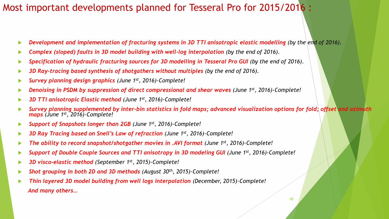
Development and implementation of fracturing systems in 3D TTI anisotropic elastic modelling (by the end of 2016).

Complex (sloped) faults in 3D model building with well-log interpolation (by the end of 2016).

Specification of hydraulic fracturing sources for 3D modelling in Tesseral Pro GUI (by the end of 2016).

3D Ray-tracing based synthesis of shotgathers without multiples (by the end of 2016).

Survey planning design graphics (June 1st, 2016)-Complete!

Denoising in PSDM by suppression of direct compressional and shear waves (June 1st, 2016)-Complete!

3D TTI anisotropic Elastic method (June 1st, 2016)-Complete!

Survey planning supplemented by inter-bin statistics in fold maps; advanced visualization options for fold; offset and azimuth maps (June 1st, 2016)-Complete!

Support of Snapshots longer than 2GB (June 1st, 2016)-Complete!

3D Ray Tracing based on Snell’s Law of refraction (June 1st, 2016)-Complete!

The ability to record snapshot/shotgather movies in .AVI format (June 1st, 2016)-Complete!

Support of Double Couple Sources and TTI anisotropy in 3D modeling GUI (June 1st, 2016)-Complete!

3D visco-elastic method (September 1st, 2015)-Complete!

Shot grouping in both 2D and 3D methods (August 30th, 2015)-Complete!

Thin layered 3D model building from well logs interpolation (December, 2015)-Complete!

And many others…

10

Most important developments planned for Tesseral Pro for 2015/2016 :

Short Intro:

In this presentation we will assess the veracity of the 3D synthetic seismograms generated in the latest version of Tesseral Pro (ver.4) and also compare them with the seismograms provided by our competitor. For this entire presentation we will be using the same P-wave velocity model for all modelling computations. We will also be using a structural surface with identical dimensions to our P-wave velocity model in the XY plane and accommodate the same survey design which was used by a our competitor.

Plan of work:

I. QC of 3D data (acquisition geometry, competitor’s synthetic gathers, 3D velocity

model).

II. Running 3D Acoustic modelling with a given survey layout for a selected shot point

on CPU.

III. Comparison of the synthetic seismograms obtained in Tesseral Pro with the

competitor’s seismograms.

IV. Running 3D Ray Tracing for a selected shot point on CPU.

V. Creating a 3D VSP Survey Design and running 3D acoustic and elastic modelling.

VI. 3D model building from .grd files.

11

Analysis/Observations: QC of 3D data

Compressional Velocity model in 3D view

12

Profile

XY PLANE

THE CORRESPONDING CROSS SECTION

Structural surface with the observation system Structural surface in 3D view

Analysis/Observations: QC of 3D data

Additional Comments:

Red square represents the chosen shot point.

Blue circles represent receivers that correspond to the selected shot point.

The chosen test shot point corresponds to the 1st shot point in our competitor’s seismogram file with the coordinates x=5424995, y=7442905. 13

Active shot point

Recording patch

Seismogram visualization

Third party gathers (AGC=450 ms, noise=0.01%) Tesseral gathers (AGC=250 ms, noise=0.01%, freq.= 30 Hz)

Additional Comments:

As we observe the high signal to noise ratio in the Tesseral seismogram makes the reflectors easily distinguishable. While the competitor’s seismogram may

illustrate more reflection events (due to a higher signal frequency), the presence of strong background noise makes it difficult to identify these as primary

reflections, multiples, reverberations or simply high frequency noise. For the best visualization an optimum AGC was assigned for each seismogram individually

and sampling rate of 4 msec. was chosen for the Tesseral Seismogram. 14

Elastic gathers (AGC=250 ms, noise=0.01%)

3D Elastic Modelling on CPU

Additional Comments:

Despite the low signal frequency of 14 Hz the generated 3D elastic seismogram displays a fairly good signal to noise ratio.

For consistency the modelling settings were kept constant (i.e. identical to the model settings from the previously ran acoustic modelling, apart from the signal

frequency) including the velocity model itself, the structural surface file and the exact same shot point.

15

Comparison between Acoustic and Elastic synthetic seismograms

generated in Tesseral Pro

3D Acoustic shot gathers (AGC=250 ms, noise=0.01%) 3D Elastic shot gathers (AGC=300 ms, noise=0.01%)

Additional Comments:

If we compare the 2 seismograms we can conclude that the reflection hyperbolas which are missing in the acoustic seismogram but are present in the

elastic seismogram are entirely due to reflections of shear and converted waves. 16

Comparison between competitor’s Acoustic and Elastic synthetic

seismograms generated in Tesseral Pro

Third party gathers Tesseral Elastic gathers

Additional Comments:

Due to presence of shear and converted waves we can identify reflection events that are not to be found in the competitor’s seismogram. The absence of high

frequency noise in Tesseral makes it THE MOST SUITABLE of all for further processing and interpretation.

17

Snapshot of wavefield propagation in a 3D velocity cube

18

3D Ray Tracing

Additional comments:

In order to test the robustness of 3D Ray Tracing in Tesseral Pro a smaller 3D Shear velocity model was selected and a suitable surface structural map was created.

3D Velocity ModelGenerated surface structural map in 3D

Surface structural map and acquisition geometry

3D arbitrary seismic survey overlaid on top of the structural surface Arbitrary recording patch of the seismic survey

3D Illumination map and ray view Illumination map 3D Ray view

Fold maps for any 3D Seismic Survey

22

Structural surface map and 3D VSP survey design

VSP azimuthal 3D survey design Fig. 18 VSP radial 3D survey design

23

3D Radial VSP Survey Design

Receivers extend all the way to the bottom of the 3D model (i.e. 3955 m) with a station increment of 50 m.

Source

Receiver(s)

Structural surface map and 3D VSP survey design

24

3D Acoustic Seismogram for 3D VSP modelling

(Signal Frequency=35 Hz, Z-Component)*

3D Elastic Synthetic Seismogram for 3D VSP modelling

(Signal Frequency=35 Hz, Z-Component)*

*Elastic seismogram

displays reflection at

non-normal incidence.

Please note the

reflection of shear and

mode converted waves

*Acoustic

seismogram

displays reflection

of P-waves at

normal incidence

Synthetic VSP seismograms

25

The generated 3D velocity cube

3D model building from .GRD files

26

GRD surfaces in 3D view (identical size in XY

plane)

3D Model building from well stratigraphy

22

Surfaces generated using Spline interpolation (please

note the numbered wells) The generated 3D velocity cube

3D thin-layered model building from well stratigraphy and

log data

Surfaces generated using Spline interpolation (please

note the numbered wells)

Surfaces generated using Spline interpolation (please

note the numbered wells)

29

Thank you for your attention!

Questions?

Comments?