3D SIMULATION OF COUPLED FLUID FLOW AND SOLID HEAT

Proceedings of ASME Turbo Expo 2010: Power for Land, Sea and AirGT2010

June 14-18, 2010, Glasgow, UK

GT2010-22513

3D SIMULATION OF COUPLED FLUID FLOW AND SOLID HEAT CONDUCTION FORTHE CALCULATION OF BLADE WALL TEMPERATURE IN A TURBINE STAGE

Fabien WlassowDT/MD/MOTurbomeca

64511 Bordes CedexFRANCE

Email: [email protected]

Florent DuchaineCFD TeamCERFACS

31057 Toulouse Cedex 1FRANCE


Gilles LeroyDT/MD/MOTurbomeca

64511 Bordes CedexFRANCE


Nicolas GourdainCFD TeamCERFACS

31057 Toulouse Cedex 1FRANCE


ABSTRACT

A critical problem in high pressure turbine of modern engineis the vane and blade reliability as it is subjected to high thermalconstraints. Actually the flow entering the turbine presents highlevel of stagnation temperature as well as great radial and cir-cumferential temperature gradients. Considering that a smallvariation of the blade temperature leads to a strong reduction ofits life duration, accurate numerical tools are required for pre-diction of blade temperature. Because of the complexity of theflow within a turbomachine, the blade wall temperature is hetero-geneous and a fluid/solid coupling may improve wall temperatureprediction. This study presents a coupling strategy of a NavierStokes flow solver and a conduction solver to predict blade tem-perature. Firstly, the method is applied to the well documentedNASA C3X configuration. The influence of the fluid/solid inter-face boundary condition is studied with regards to the wall tem-perature and heat flux prediction as well as to the computationalefficiency. The predicted wall temperature is in good agreementwith the experimental results. The method is finally applied tothe prediction of the blade temperature of a high pressure tur-bine representative of a modern engine. Adiabatic and coupledresults are compared and discussed.

NOMENCLATUREA SYMBOLSC Heat capacity (J.kg-1.K-1)L Characteristic length scaleN Number of point of the fluid/solid interfaceN Number of CHT cycleP Pressure (Pa)PS Pressure sideR CHT calculation convergence criterionS Surface distance over arc lengthSS Suction sideT Temperature (K)Ts Static temperature (K)T* Coolant temperature (K)h Heat transfer coefficient (W.m-2.K-1)k Parameter of the mixed boundary conditionn Number of iterations of the solvery+ Normalized wall distanceα Period of exchange between the two codes∆t Time step of the solverΦ Heat flux (W.m-2)Γ Fluid/Solid interfaceρ Density (kg.m-3)τ Characteristic time scale (s)

1 Copyright c© 2010 by ASME

B SUPERSCRIPTI Point of the fluid/solid interfacen Fluid or solid iteration

C SUBSCRIPTaw Adiabatic wallc Convective parameterf Fluidi Total variables Solidw Wall

D ACRONYMSCHT Conjugate Heat TransferLES Large Eddy SimulationRANS Reynolds-Averaged Navier Stokes

INTRODUCTIONIn order to increase the thermodynamic efficiency of gas tur-

bine engines, the turbine inlet temperature has been continuallyincreased up to reach levels of the order of magnitude of the highpressure turbine vanes and blades melting temperatures. More-over because of the mixing within the combustor and its frame-work characteristic, the temperature and pressure fields at theturbine inlet exhibit azimuthal and radial non-uniformity knownas hot streaks. Thus the prediction of the heat load and wall tem-perature is essential for the estimation of the turbine componentslife duration. Since experimental data are difficult to collect forreal operating conditions, designers often rely on numerical sim-ulation.

Hence many authors studied the effects of hot streaks on tur-bines. Several experimental studies have been carried out on theeffects of inlet total temperature and total pressure profiles [1–4].Compared with uniform inlet profiles, a modification of the tem-perature field was observed especially near the hub and tip cor-ners. This modification of the temperature field was ascribedto the secondary flows which are driven by the inlet total pres-sure gradient [5]. The hot streaks migration in the rotor stagewas mainly studied using unsteady Reynolds-Averaged NavierStokes (RANS) simulations [6, 7] which helped to identify andunderstand the preferential migration of the hot streak towardthe pressure side of the rotor blade. This result was later used byDorney and Gundy-Burlet [8] and He et al. [9] to reduce the ro-tor heat load by arranging the clocking between hot streaks andvanes in such a way that the hot streaks impinge on the vanesleading edges.

All these studies have helped to understand the migrationof hot streaks in turbine stages and its influence on the turbineheat load, however these simulations are not sufficient to predictthe wall temperature of rotor blades. Actually, because of thehot streaks migration, the blade surface temperature varies spa-tially and temporally. Thus it is not possible to specify a priorithe blade surface temperature. Hence it is necessary to couple aflow solver with a conduction solver to predict the blade surface

temperature. Such calculations are known as Conjugate HeatTransfer (CHT) simulations. Two main approaches were usedto envestigate CHT problems in the field of turbomachinery. Thefirst one is a direct coupling where the entire system of equa-tions in the fluid and solid is solved simultaneously by a mono-lithic solver [10, 11]. The main advantage of this strategy is thatthe continuity of the temperature and heat flux at the fluid/solidinterface is implicitly guaranteed. Luo and Razinski [12] usedthis approach to predict the metal wall temperature of the NASAC3X vane using different turbulence models and Agostini andArts [13] investigate the heat transfer in a rib-roughened channelrepresentative of an internal vane cooling system. The second ap-proach consists in solving each set of field equations separatelywith dedicated solvers that exchange boundary conditions at theirinterfaces [14–16]. This solution has the advantage to solve fluidand solid equations using existing state-of-the-art codes whichhave been extensively validated. However it requires to exchangethe boundary conditions between the two solvers in an accurateand stable fashion. Hence special attention is required to set upthe coupling methodology between the codes. Heselhaus andVogel [17] attempted such calculations for a turbine cascade andshow the difference in wall temperature with an adiabatic sim-ulation. Sondak and Dorney [18] used an unsteady flow solvercoupled with an unsteady conduction solver in order to capturethe temporal evolution of a rotor blade temperature. More re-cently Duchaine et al. [19] developed a strategy to couple a LESsolver with a conduction solver in a parallel framework.

The present study investigates strategies to couple efficientlyRANS and URANS flow solvers with a conduction solver in or-der to predict turbine blade surface temperature. The influence ofthe exchanged variables as well as the synchronization betweenthe solvers are studied. The coupling methodology is evaluatedon the well documented NASA C3X test case [20] and then ap-plied to a high pressure turbine representative of an actual he-licopter engine. For the latter case, two-dimensional inlet totaltemperature and total pressure fields representative of an com-bustor exit are imposed and an unsteady RANS flow solver isconsidered in order to take into account both the migration of hotstreaks in the vane passage and in the rotor passage. Firstly theNASA C3X test case is presented. Then the CHT methodologyis described. This methodology is assessed with the NASA C3Xtest case in a third part. Finally, results for a turbine stage arepresented.

TEST CASEThe test case used to assess the CHT methodology is the

well documented NASA C3X cooled turbine cascade reportedby Hylton et al. [20] and presented Fig. 1. The experimentalcascade employed three cooled vanes made of ASTM310 stain-less steel and the center vane is instrumented for heat transferand aerodynamic measurements. The vane geometric character-istics and the solid thermal properties are presented respectivelyin Tab. 1 and 2. The cooling system corresponds to ten holesfor which the hole diameter, the averaged coolant temperatureand flow rate were measured and are presented in a NASA re-


Figure 1. NASA C3X MESH FOR CONDUCTION SIMULATION

Table 1. CASCADE GEOMETRY

Setting angle (◦) 59.89

Air exit angle (◦) 72.38

Vane height (m) 0.07620

Vane spacing (m) 0.11773

True chord (m) 0.14493

Axial chord (m) 0.07816

Table 2. THERMAL CHARACTERISTICS OF ASTM310

Thermal conductivity (W.m-1.K-1) ks 6.811+0.020176∗T

Heat capacity (J.kg-1.K-1) Cs 586.15

Density (kg.m-3) ρs 7900.0

port [20]. Associated heat transfer coefficients were calculatedfrom Nusselt number correlation for turbulent flow. The centervane is instrumented with pressure taps and thermocouples. Thethermocouples are located in the fully two dimensional regionof the vane near midspan and additional thermocouples were in-stalled off midspan to check the 2-D assumption. Pressure tapsare located near midspan. Experimental results were obtainedover a wide range of operating conditions. The run 158 was se-lected for this study. The operating conditions are presented inTab. 3.

Table 3. OPERATING CONDITIONS FOR RUN 158

Inlet Total temperature (K) 808.0

Inlet Total pressure (Pa) 243700.0

Inlet Mach Number 0.17

Outlet Mach Number 0.91

Inlet Turbulence level (%) 8.3

METHODOLOGYThis section presents the methodology used to perform the

CHT simulation. The flow and conduction solvers are first pre-sented. Then, the coupling strategy is described.

Flow solverThe flow solver used for this study is the elsA software

developed by ONERA and CERFACS [21]. This is a finite vol-ume cell centered code that solves the RANS or LES equationson multi-block structured meshes. The elsA software is able totake advantage of modern massively parallel platforms [22]. Forthis study a second order Roe scheme with a Harten entropiccorrection is used to compute convective fluxes and a secondorder centered scheme is used for the diffusive fluxes. The two-equation k− l model of Smith [23] is used to compute the eddyviscosity. Local transition criteria such as the Abu-Ghannam andShaw criterion [24] may be used for transition. For steady flowcalculations, an implicit time integration is achieved througha backward Euler scheme coupled with a scalar LU-SSORmethod [25].

For the NASA C3X mesh a HOH topology is used. The Oblock contains 125, 53 and 5 points respectively in the stream-wise, pitchwise and spanwise direction. Only few points are usedfor the spanwise direction since the experiment [20] report a fully2-D flow. It corresponds to a height of 0.01 m in the spanwise di-rection. The full domain has 84,885 points (Fig. 2). The averagey+ around the vane is 0.55. 8 power units of an IBM IDATA-PLEX system were used for the flow simulation.

Conduction solverThe conduction solver is the AVTP code developed at

CERFACS. It solves the transient conduction in solid domainsdescribed by the energy conservation. The parallel imple-mentation of AVTP on unstructured grids allows to solve heatconduction on complex geometries. The code takes into accountchanges of heat capacity and conductivity with temperatureusing analytical laws. The numerical integration uses either acell-vertex finite volume 4∆ operator or a finite element Galerkin2∆ operator [26]. The explicit scheme provides second-orderaccuracy on hybrid meshes.

A view of the NASA C3X solid mesh is presented on


Figure 2. NASA C3X MESH FOR FLOW SIMULATION

Table 4. COOLANT TEMPERATURE AND HEAT TRANSFER COEFFI-CIENT FOR EACH COOLING HOLE

hole T (K) h (W.m-2.K-1)

1 358.14 1409

2 359.37 1458

3 349.97 1549

4 351.51 1392

5 342.56 1456

6 371.85 1403

7 351.85 1365

8 385.96 1974

9 413.22 1388

10 454.87 1742

Fig. 1. This mesh contains about 2 millions of tetrahedral cellswhich is clearly over discretized. However, since the solidconduction computation is fast, this mesh was nevertheless used.The computation was performed using 32 computing units ofa IBM IDATAPLEX system. The spanwise dimension of theconduction mesh corresponds to the one of the fluid domainmesh and periodicity is enforced in this direction since theexperimental results report a 2-D problem. The choice has beendone not to solve a purely 2-D problem as for the two solversthe gain in CPU time between a 2-D and a 3-D problem isrelatively small. Moreover, the methodology was developped to

handle 3-D problems. Since the internal flow is not solved, theboundary conditions on the cooling holes walls were specifiedusing a Fourier condition based on the coolant temperatures andheat transfer coefficient presented in Tab. 4. The positions of theholes are showed on Fig. 1.

Coupling strategyThe resolution of CHT problems involves taking into

account multiple questions. Among them, two main issues wereconsidered for the present work:

- For CHT problems, the way to synchronize the solvers andthe frequency of the exchanges between the codes influence thestability as well as restitution time of the computations but theyare primarily imposed by the physics of the problem. In fact theratio between the characteristic time scale of the solid (diffusivetime scale τs) and fluid (convective time scale τ f ) problems isthe key parameter. Hence if the characteristic time scale for thesolid and fluid problems are of the same order of magnitude thenan unsteady behaviour of the fluid problem may induce an un-steady response of the solid. In that case the codes have to becoupled in a strong way, that is to say, the shared variables haveto be exchanged with a time coherence so that an unsteady CHTproblem will be described. However if one of the time scale ismore than one order of magnitude greater than the other one thencode sequencing is sufficient and the CHT calculation will reacha steady state of the coupled problem. The last situation is repre-sentative of CHT problems in turbines where the solid time scaleis much larger than the fluid one. Hence for the NASA C3X caseτs and τ f are defined by Eqn. 2.

τs =ρsCsL2

s

ks(1)

τ f =L f

U(2)

where Ls is the minimal distance between the solid skin surfaceand a cooling hole and L f is the axial chord of the vane. Sinceτsτ f

= 500 the solid can be assumed to be in a steady state. Thuscode sequencing is sufficient to tackle the coupled heat transferproblems treated within this work. Then the choice of the ex-change frequency between the codes is not driven by physicalconsideration but only by numerical ones. Since a steady flowsimulation is considered, there is no physical time coherence forthe fluid problem. Thus at each CHT cycle the steady flow sim-ulation will be performed until convergence. On the contrary, anunsteady conduction solver is considered so that there is a phys-ical time coherence within the solid problem and the frequencyof exchange of the two codes can be related to τs. The frequencyof exchange is 1

α with α defined by Eqn. 3.

α =ns∆ts

τs(3)


Figure 3. CHT CALCULATION FLOWCHART

where ∆ts and ns are respectively the conduction solver time stepand number of iterations. The flowchart of the CHT calculationassociated with this sequential procedure is presented on Fig. 3.Based on this flowchart, the parameter α can be adjusted toimprove the convergence rate of the CHT calculation. A smallvalue of α can be regarded as a good thing for convergencebecause, at each CHT cycle, the conduction solver has no time toreach a final state which is wrong since the boundary conditionshave not converged yet. However a great number of CHT cycleswill be required since a certain time is needed anyway to let thetemperature diffuse in the solid. Moreover when a great numberof CHT cycles is considered the cost of the data exchanges maynot be negligible anymore.

- The boundary conditions applied to the fluid and solidcodes, including the variables shared by the codes, are criticalfor the precision and stability of the computations.

At a fluid/solid interface Γ f s where thermal properties arediscontinuous, heat flux and temperature are continuous. As aconsequence, the local heat flux and the temperature must beequal on the interface in the solid and fluid parts:

{φI

f = φIs

T If = T I

s, I ∈ Γ f s (4)

with φIf , φI

s the fluid and solid heat fluxes at the interface point Iand T I

f , T Is the fluid and solid temperatures at the same location.

Thus, the natural variables to share between the codes are φ andT at the interfaces. From now on, the notation I will be droppedfor clarity reasons. However shared variables will still be localvariables at a point of the interface Γ f s.

Previous studies [27–29] have shown that a good choice toinsure stability under some conditions is to impose the heat fluxcomputed in the fluid part to the solid domain through a Neu-mann boundary condition and the temperature of the solid sur-face as Dirichlet condition to the fluid frontier. Nevertheless,to reach a converged thermal state, the heat flux computed with

the fluid solver will be imposed to the solid boundary on a largenumber of solid iterations ns. The imposition of a constant heatflux Φ on a surface S will lead to a linear time derivation of thetotal energy E(t) of the structure during the interval t − t0 thatcorresponds to the ns iterations:

E(t) = E(t0)+Φ ·S · (t− t0) (5)

Such derivations at each update of the solid boundary conditionslead to spurious oscillations of the fluxes and temperatures. Thisnumerical instability often grows and causes a fail of the compu-tation.

Several solutions were proposed in the literature to over-come this type of instability. Sondak and Dorney [18] rewriteEq. 4 as:

{k f−−→gradTf = ks

−−→gradTs

Tf = Ts(6)

and then estimate the temperature gradient with finite differ-ences. Hence the system of equations can be solved for T andDirichlet boundary conditions can be imposed on both the fluidand solid solvers. However, when dealing with different kindof grids (structured/unstructured) for the solid and fluid solvers,a first order finite difference expression may not be accurateenough to estimate the temperature gradients at the fluid/solidinterface. In this paper it has been chosen to use the heat fluxescalculated with the schemes of each solver in order not to altertheir accuracy. Other solutions were used to overcome the prob-lem of numerical instabilities. For instance, one can use a relax-ation based on a convective formulation of the heat flux. Indeed,in the heat transfer community, the heat flux at the surface of astructure φn

s is often express as a Fourier boundary condition:

φns = hc(T n

s −Tc),with n = 1,ns (7)

with hc and Tc are the convective heat transfer coefficient andconvective temperature respectively. In this formulation, the fluxφn

s and the temperature T ns evolve during the iterations leading to

the convergence to a steady state between two consecutive up-dates of Tc and hc. The convective parameters are determinedwith the heat flux computed in the fluid φ f and the temperatureof the wall surface Tf :

hc(Tf −Tc) = φ f (8)

Eqn. 8 must be augmented by a way to determine either hc or Tc.The idea is to fix hc or Tc and then to determine the correspondingvalue of Tc or hc with Eqn. 8. Generally Tc is chosen as the bulktemperature.

For turbomachinery applications, the evolution of the flowfield and the boundary layer along the blade prevent a trivial de-termination of the convective parameters. Instead of using the


total inlet temperature Tt0, Tc can be approximated by Taw whichrepresents the surface temperature of a perfectly insulated sur-face and it is obtained from an adiabatic flow simulation. Themain problem when using a given temperature Tc and then usingEqn. 8 to determine hc is that the procedure can give negativevalues of the heat transfer coefficient. These non physical valuesof hc may lead the computation to fail due to numerical instabil-ities. In order to avoid negative values of hc, one can choose tofix the heat transfer coefficient and compute Tc with Eqn. 8. Theheat transfer coefficient depends on several parameters but pri-marily on the thickness and nature of the boundary layer. Indeed,thin boundary layers conduct more heat that thick ones. Turbu-lent boundary layers transfer more heat per unit of thickness thando laminar ones [30]. Assuming that local hc is only a functionof the aerodynamic field, its determination remains not trivial.From experimental point of view, measurement methods of de-tailed heat transfer coefficient involve heat-mass transfer anal-ogy, liquid crystal and infrared thermography [31–33]. Numeri-cal prediction with CFD solvers of hc requires several numericalsimulations of the flow field and/or experimental data [32, 34].

Another solution consists in rewriting the continuity of heatflux and temperature across the interface (Eqn. 4) in the follow-ing form:

{Tf = Ts

φ f + kTf = φs + kTs(9)

with k a numerical relaxation parameter. The resulting boundarycondition for the structure, called mixed condition, looks :

φns = φ f + k(Tf −T n

s ),with n = 1,ns (10)

As underlined in the case of the Fourier condition (Eqn. 7), bothφn

s and T ns of the mixed formulation converge to a steady state

between two consecutive updates of φ f and Tf . The stabilityof the mixed condition for the solid domain used in conjunctionwith Dirichlet boundary temperature for the fluid depends on thevalue of k (when k tends to 0, the mixed formulation tends to theNeumann condition) and on the exchange frequency. Note thatat convergence, Tf = T n

s so that the mixed condition tends to thethermal equilibrium given by Eqn. 4.

The boundary conditions for the coupled problem tested dur-ing this work are listed in Table 5. The objective was to checkthe unicity of the solution obtained with different sets of bound-ary conditions in order to choose the best suited for the industrialcase.

The convergence is monitored on the criterion R , definedby Eqn. 11 which control the evolution of the temperature of Γ f sbetween two CHT cycle N and N +1.

R =|T N+1

s −T Ns |max

1N ∑N

i=1 T N+1s

(11)

Since the flow and conduction solvers use different meshes threedimensional linear interpolations are used when the shared vari-ables are exchanged.

APPLICATION TO THE ACADEMIC NASA C3X CASEMethodology

The coupling strategy for CHT problems is assessed on theNASA C3X case. Firstly, the four cases of boundary conditionsfrom Tab. 5 are evaluated and compared. The results obtained forthe different boundary conditions for the wall temperature andthe convective heat transfer coefficient are presented Fig. 4. Forcomparability, the convective heat transfer coefficient presentedfor all boundary conditions is calculated with Tre f = 811K. One

540560580600620640660680700

-150 -100 -50 0 50 100 150 200T

w

S

← Suction side →← Pressure side →

ABCD

020040060080010001200

-150 -100 -50 0 50 100 150 200

hc

S


ABCD

Figure 4. BOUNDARY CONDITION INFLUENCE

can see that all boundary conditions give the same results so thatthe choice of the boundary condition will be based only on prac-tical and computational efficiency criteria. Hence the mixed con-dition is preferred as no preliminary computations or experimen-tal study is required as for the Fourier condition with Taw as refer-ence temperature or a fixed local convective heat flux coefficient


Table 5. BOUNDARY CONDITIONS FOR CHT PROBLEMS

Fluid Solid Case

Dirichlet T nf = Ts

Fourier: φns = φ f

Tre f−Tf(T n

s −Tre f ) A

Fourier: φns = φ f

Taw−Tf(T n

s −Taw) B

Fourier: φns = hre f (T n

s −Tf ) C

Mixed: φns = φ f + k(Tf −T n

s ) D

and no question about the reference parameters is raised. Fig-ure 5 shows the convergence criterion for all type of boundarycondition plotted (in logscale) against the number of CHT cy-cles. It shows that the convergence is the same for the four kindsof boundary condition. The mixed boundary condition parame-ter k used for this comparison is k = 100. As explain below, thisvalue of k gives almost the best convergence rate as maintainingstability.

1e-051e-040.0010.010.1

0 20 40 60 80 100 120 140 160 180 200

R

CPU time (hours)

ABCD

Figure 5. CONVERGENCE OF THE CHT CALCULATION

The parameter k of the mixed boundary condition can be ad-justed in order to accelerate the convergence while maintainingthe stability of the computations. One can observe that when thisparameter decreases, the convergence rate increases. Howevertoo small values of k can lead to an unstable coupled systemwhen used with unsuitable exchange frequency [19,28,29]. Fourdifferent values of k (50, 500, 5000 and 50000) were tested.Figure 6 shows the convergence rate for these four cases andone can verify that the case k = 50 converges more rapidlyeven if the gain compared with the case k = 500 is small. Theconvergence acceleration when decreasing k is not linear andfor small values of k, typically lower than 500, the convergencerates are of the same order magnitude.

The influence of the exchange frequency, defined by Eqn. 3,

1e-081e-071e-061e-051e-040.0010.010.1

0 50 100 150 200 250 300R

CPU time (hours)k = 50k = 500k = 5000k = 50000

Figure 6. INFLUENCE OF k ON THE CHT SIMULATION CONVER-GENCE

1e-051e-040.0010.010.11

0 100 200 300 400 500 600

R

CPU time (hours)

α = 10

α = 20

α = 40

α = 80

Figure 7. INFLUENCE OF α ON THE CHT SIMULATION CONVER-GENCE

was also evaluated by changing the number of iterations of theconduction solver. Four cases were studied : α = 10, 20, 40 and80. Figure 7 shows the convergence of the CHT calculations forthese four value of α. At the beginning of the CHT computation,the convergence rate is faster with small value of α. At that point,


the shared variables are wrong with regards to the convergedstate. So it is important to often update them in order to avoidwasting computational time solving a problem with inaccurateboundary conditions and so to speed up the convergence. How-ever one can see that when R has reach a level of 10-4 the conver-gence rate starts being faster for medium value of α. The reasonis that now the value of the shared variables is closed to the con-verged state and the information imposed through the boundaryconditions has to propagate within the solid domain. So a greaternumber of iterations is required at each CHT cycle for the con-duction solver. For α = 80 the computation is inefficient becausetoo much time is spend for the conduction calculation. Based onthis study, it may be interesting for computational efficiency toadjust the parameter α in function of the convergence criterionduring the computation.

Comparisons with experimental results

540560580600620640660680700

-150 -100 -50 0 50 100 150 200

Tw

S


CHT al ulation without transitionCHT al ulation with transitionExperimental data of Hylton et al

020040060080010001200

-150 -100 -50 0 50 100 150 200

hc

S


CHT al ulation without transitionCHT al ulation with transitionExperimental data of Hylton et al

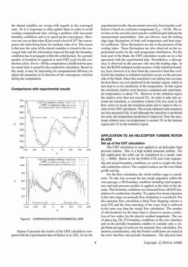
Figure 8. COMPARISON WITH EXPERIMENTAL DATA

Figures 8 presents the results of the CHT calculation com-pared with the experimental data of Hylton et al. [20]. As for the

experimental results, the presented convective heat transfer coef-ficient is based on a reference temperature Tre f = 811K. The er-ror bars on the onvective heat transfer coefficient plot indicate themeasurements uncertainties. One can observe, near the trailingedge large fluctuations in both wall temperature and heat trans-fer coefficient. These fluctuations are due to the presence of thecooling holes. These fluctuations are also observed on the ex-perimental results for the wall temperature distribution. For themain part of the blade, the CHT calculation results are in a fairagreement with the experimental data. Nevertheless, a discrep-ancy is observed on the pressure side near the leading edge. Infact, the RANS turbulent model assumes a fully turbulent bound-ary layer, however it is clear from the convective heat flux coef-ficient that laminar to turbulent transition occurs on the pressureside of the blade. Since this transition is not taking into account,the heat fluxes are over predicted in the laminar region, which inturn lead to a over prediction of the temperature. In that regionthe maximum relative error between computed and experimen-tal temperatures is about 7%. However in the turbulent regionthe relative error does not exceed 2%. In order to take into ac-count the transition, a correlation criteria [24] was used in theflow solver to locate the transition point and to improve the re-sults of the CHT calculation. The results obtained with transitionare also presented Fig. 8 and although the transition is predictedtoo early, the temperature prediction is improved. Now the max-imum relative error on temperature is around 3% in the laminarregion and 1% in the turbulent region.

APPLICATION TO AN HELICOPTER TURBINE ROTORBLADESet up of the CHT calculation

The CHT calculation is now applied to an helicopter highpressure turbine. This is a high loaded transonic turbine. Forthis application the solid can be considered in a steady state( τs

τ f= 4000). Hence as for the NASA C3X case code sequenc-

ing and mixed boundary conditions are used to couple the flowand conduction solvers. The coupled surfaces are the rotor bladeprofile and tip.

For the flow calculation, the whole turbine stage is consid-ered. To take into account the hot streak migration within thevane passage, a 2D boundary condition including total tempera-ture and total pressure profiles is applied at the inlet of the do-main. This boundary condition was extracted from a RANS sim-ulation of a combustion chamber. To capture hot streak migrationin the rotor stage, an unsteady flow simulation is considered. Forthis unsteady flow calculation a Dual Time Stepping scheme isused [35] and the time marching of the inner loop is achievedin the same way than the steady flow calculation. The numberof sub-iterations for the inner loop is chosen to ensure a reduc-tion of two orders for the density residual magnitude. The useof phase-lag [36, 37] boundary conditions at the rows interfaceand on the periodic boundaries enables to consider only a sin-gle blade passage of each row for unsteady flow calculation. Formemory consideration, only the Fourier coefficients are stored atthe rows interface and periodic boundaries. The physical time


step is chosen so that 200 iterations and 510 iterations are setto solve the blade passing frequency of the opposite row respec-tively in the stator and rotor frame of reference. For the flow, oneCHT cycle corresponds to the time required for the rotor blade totraverse the vane passage. The variables shared by the flow solverwith the conduction code are < Tf > and < φ f >, where <> de-notes time averaged quantities over one CHT cycle. Thanks tothe phase-lag method, only one vane passage and one rotor pas-sage are considered, each meshed using a O6H topology. 175,49 and 89 points are present in the vane mesh respectively in thestreamwise, pitchwise and spanwise direction and 109, 49 and109 for the rotor mesh with 33 points in the radial tip gap. Thewhole mesh contains 3.5 millions of nodes and the average y+ is0.53. A view of the mesh is presented on Fig. 9. The fluid flowcalculation was initialized with an unsteady RANS adiabatic so-lution in order to save the time required for the periodic flow toestablish.

For the solid part only the rotor blade is considered. Thisis an uncooled blade with a fir-tree blade root which is consid-ered for the conduction simulation. It is important to considerthe fir-tree root, as a part of the heat fluxes exchanged with theflow will exit through the root. The bottom of the fir-root is setas an isothermal surface. Except the isothermal and the coupledboundaries, every other surfaces are considered adiabatic. Actu-ally, for the real case, the fir-root side surfaces are exchangingheat with the rest of the engine. To model this phenomenon,it would require to simulate the whole system since the thermalconditions here are not known. So it has been assumed that all theheat transfered from the fluid to the hub surface is then transferedto the rest of the engine through the fir-root side surface whichmeans that the heat flux budget between these surfaces is zero.Thus the fir-root side surface and the hub are set as adiabatic sur-faces. The mesh for this blade contains 190 077 tetrahedral cells.Most of the cells are located in the blade profile so that the num-ber of elements used to discretize the blade surface for both theflow and the conduction solver are close. In fact, for the bladesurface there are 16 159 triangular elements on the solid mesh

Figure 9. MESH OF THE ONE STAGE TURBINE

Figure 10. TURBINE STAGE CHT CALCULATION FLOWCHART

Figure 11. CONVERGENCE OF THE CHT CALCULATION OF THEROTOR BLADE

and 16 125 quads on the fluid mesh. Thus, errors due to the lin-ear interpolations are reduced. Figure 10 sums up the flowchartof the CHT calculation of the high pressure turbine. The con-vergence was monitored for the flow and conduction solvers aswell as for the coupled interface. For the flow solver, the mass-flow rates and static temperatures at the inlet and outlet of eachrow were analysed using windowed Fourier transform. The timeevolution of the energy spectrum and harmonic amplitudes wasmonitored to verify a periodic state was reached. For the con-duction solver, the time evolution of the minnimum, maximumand average temperature was observed until a steady state wasreached. Finally, the criterion R (Eqn. 11) was supervised untilit reaches 10-3 (Fig. 11). About 40 CHT cycles were necessaryto converge the coupled interface which represents about 2000CPU hours on the IBM IDATAPLEX system.


Figure 12. STATIC TEMPERATURE IN THE TURBINE STAGE - TOP:ADIABATIC SIMULATION, BOTTOM: CHT SIMULATION

ResultsFigure 12 shows the hot streak migration within the turbine

stage at 4 different axial planes. The typical effects of hot streakmigration are observed. Actually, a radial migration along thevane span and towards the shroud is observed in the vane pas-sage. In the rotor passage the preferential migration of hot fluidtowards the pressure side, the segregation effect, is captured aswell as the redistribution of hot fluid on suction side due to thetip leakage flow near le trailing edge. The results are comparedwith those of an adiabatic wall simulation. The consideration ofthe solid in the problem does not really influences the hot streakmigration as shown by Fig. 12. Only slight modifications of thefluid temperature field are observed, in particular close to thepressure side of the rotor blade. For the CHT case, the radial ex-tension of the hot streak near the pressure side of the rotor bladeis slightly reduced. In fact, modifications of the fluid temperaturefield are observed in thermal boundary layer and close to it butnot in the middle of the passage. However the influence on thewall blade temperature is important. Figure 13 shows the relativedifference the adiabatic wall temperature and the wall tempera-ture predicted by the CHT simulation. This difference is definedby Eqn. 12.

∆T/T =TCHT −Taw

TCHT(12)

The average temperature of the blade is about 1.9% cooler forthe CHT simulation. It may represent a great reduction of theblade’s life duration. However the cooling of the blade is het-erogenous. Actually, the CHT calculation predicts a lower walltemperature near the hub mainly because the heat is transportedin the fir-tree of the blade. Around the blade profile, the CHTcalculation predicts higher temperatures for the region where theblade is thin, and lower temperatures where the blade is thicker,

Figure 13. RELATIVE DIFFERENCE BETWEEN WALL TEMPERA-TURE PREDICTED BY AN ADIABATIC AND A CHT CALCULATION

obviously since the temperature will diffuse more where the solidis thicker.

CONCLUSIONA coupling strategy used to handle CHT problems typical of

high pressure turbine cases was described. As the characteristictime scale of the solid is several order of magnitude greater thanthe one of the fluid, the solid is considered as in a steady stateand only code sequencing is considered.

For the coupling methodology the choice of the fluid/solidboundary condition was particularly studied on the well docu-mented NASA C3X case. Three different Fourier boundary con-ditions, based on different reference temperatures or convectiveheat transfer coefficients, and a mixed boundary condition werecompared. It has been shown that these boundary conditions donot influence the final prediction of the wall vane temperature.However for Fourier type boundary conditions, the choice of areference temperature or convective heat transfer coefficient isnot straightforward and may lead to non-physical behaviours andoften requires additional computations. Thus the mixed bound-ary condition was chosen for the second part of the study. Com-putational time reduction can be achieved by reducing the pa-rameter k of the mixed boundary condition, however below 500no real gain is obtained. Finally, the influence of the exchangefrequency between the flow and the conduction solver was stud-ied. At the beginning of the CHT calculation, a high exchangefrequency is required so that the correction enforced on the heatflux and temperature at each CHT cycle is not too important.However, when the solution has already started to converge theexchange frequency can be reduce to let time for the temperatureto diffuse within the solid.

The results of the CHT calculation for the NASA C3X caseconcerning the wall temperature and the convective heat trans-fer coefficient were compared with experimental data, showinggood agreement. The results have been improved by taking intoaccount boundary layer transition in the flow solver. The aver-age error was around 1% with a maximum of 3% near the lead-ing edge when the transition was taken into account. The CHTmethodology was then applied to a turbine rotor blade. For thiscase, the whole turbine stage was considered in the flow solver


using an unsteady RANS approach in order to capture hot streakmigration and to predict a realistic blade temperature distribu-tion. The comparison with a temperature distribution resultingfrom an adiabatic simulation shows differences that are locallymore than 5% which is important for the life duration predictionof the blade.

The CHT strategy can now be used to study in more detailthe influence of coolant injections in high turbine pressures andtheir influence on the blade temperature. The coolant injectionshave only to be taken into account by the flow solver and theCHT strategy can be applied and give more realistic results thana simple adiabatic flow simulation. One major assumption inthis work is that the solid is in a steady state with regards to thefluid. In order to validate the choice of code sequencing, furtherstudies would include unsteady coupling strategy were the fluidand solid solvers will be coupled with time coherence.

ACKNOWLEDGMENTThe authors are grateful to Turbomeca for permission to

publish results on their configurations and for their support in thisstudy. Special thanks to the CERFACS - CFD Team for develop-ing efficient numerical methods for the elsA and AVTP softwaresas well as for their availability for discussions concerning numer-ical methods. The authors are also grateful to the elsA softwareteam (ONERA).

REFERENCES[1] Schwab, J. R., Stabe, R. G., and Whitney, W. J., 1983. “An-

alytical and experimental study of flow through an axial tur-bine stage with a nonuniform inlet radial temperature pro-file”. AIAA Paper 83-1175.

[2] Stabe, R. G., Whitney, W. J., and Moffitt, T. P., 1984. “Per-formance of a high-work low aspect ratio turbine with arealistic inlet radial temperature profile”. AIAA Paper 84-1161.

[3] Barringer, M., Thole, K., Polanka, M., Clark, J., and Koch,P., 2009. “Migration of combustor exit profiles throughhigh pressure turbine vanes”. J. Turbomach., 131, April,pp. 021010–10.

[4] Barringer, M., Thole, K., and Polanka, M., 2009. “An ex-perimental study of combustor exit profile shapes on end-wall heat transfer in high pressure turbine”. J. Turbomach.,131, April, pp. 021009–10.

[5] Hawthrone, W. R., 1951. “Secondary circulation in fluidflow”. Proc. R. Soc. London, Ser. A, 206, pp. 374–387.

[6] Dorney, D., Davis, R., and Edwards, D., 1992. “Unsteadyanalysis of hot streak migration in a turbine stage”. J.Propul. Power, 8, pp. 520–529.

[7] Takahashi, R., and Ni, R.-H., 1991. “Unsteady hot streakmigration through a 1 1/2-stage turbine”. In AIAA Paper,no. 91-3382.

[8] Dorney, D., and Gundy-Burlet, K., 1996. “Hot-streakclocking effects in a 1-1/2 stage turbine”. J. Prop. Power,12, pp. 619–620.

[9] He, L., Menshikova, V., and Haller, B. R., 2004. “Influ-ence of hot streak circumferential length-scale in transonicturbine stage”. In ASME TURBO EXPO 2004: Interna-tional Gas Turbine & Aeroengine Congress & Exhibition,no. GT2004-53370.

[10] Kao, K. H., and Liou, M. S., 1997. “Application ofchimera/unstructured hybrid grids for conjugate heat trans-fer”. AIAA Journal , 35(9), pp. 1472–1478.

[11] Han, Z. X., Dennis, B., and Dulikravich, G., 2001. “Simul-taneous prediction of external flow-field and temperature ininternally cooled 3-d turbine blode material”. Int. J. TurboJet-Eng. , 18, pp. 47–58.

[12] Luo, J., and Razinsky, E. H., 2007. “Conjugate heat transferanalysis of a cooled turbine vane using the v2f turbulencemodel”. J. Turbomach., 129(4), pp. 773–781.

[13] Agostini, F., and Arts, T., 2005. “Conjugate heat trans-fer investigation of rib-roughened cooling channels”. InProceedings of ASME Turbo Expo 2005, no. ASME PaperGT2005-68116.

[14] Montenay, A., Pate, L., and Duboue, J. M., 2000. “Conju-gate heat transfer analysis of an engine internal cavity”. InProceedings of ASME Turbo Expo 2000, no. ASME Paper2000-GT-282.

[15] Verdicchio, J., Chew, J., and Hills, N., 2001. “Coupledfluid/solid heat transfer computation for turbine discs”. InProceedings of ASME Turbo Expo 2001, no. ASME Paper2001-GT-0205.

[16] Amaral, S., Verstraete, T., den Braembussche, R. V., andArts, T., 2010. “Design and optimization of the internalcooling channels of a high pressure turbine blade - part i:Methodology”. J. Turbomach., 132(021013).

[17] Heselhaus, A., and Vogel, D. T., 1995. “Numerical sim-ulation of turbine blade cooling with respect to blade heatconduction and inlet temperature profiles”. In ASME, SAE,and ASEE, Joint Propulsion Conference and Exhibit, 31st,no. AIAA-1995-3041.

[18] Sondak, D. L., and Dorney, D. J., 2000. “Simulation of cou-pled unsteady flow and heat conduction in turbine stage”. J.Propul. Power, 16(6), pp. 1141–1148.

[19] Duchaine, F., Mendez, S., Nicoud, F., Corpron, A.,Moureau, V., and Poinsot, T., 2009. “Coupling heat transfersolvers and large eddy simulations for combustion applica-tions”. Int. Journ. of Heat and Fluid Flow, 30(6), Decem-ber, pp. 1129–1141.

[20] Hylton, L., Mihelc, M., Turner, E., Nealy, D., and York,R., 1983. Analytical and experimental evaluation of theheat transfer distribution over the surfaces of turbine vanes.Tech. Rep. CR 168015, NASA.

[21] Cambier, L., and Veuillot, J., 2008. “Status of the elsa cfdsoftware for flow simulation and multidisciplinary applica-tions”. In AIAA, Aerospace Sciences Meeting and Exhibit,46 th, AIAA 2008-664.

[22] Gourdain, N., Montagnac, M., Wlassow, F., and Gazaix,M., to be published. “High performance computing tosimulate large scale industrial flows in multistage compres-sors”. Int. Journal of High Performance Computing.


[23] Smith, B., 1990. “The k - kl turbulence model and walllayer model for compressible flows”. In AIAA Paper,no. 90-1483, 21st Fluid and Plasma Dynamics Conference.

[24] Abu-Ghannam, B. J., and Shaw, R., 1980. “Natural transi-tion of boundary layers. the effects of turbulence, pressuregradient, and flow history”. J. Mech. Engr. Science, 22(5),pp. 213–228.

[25] Yoon, S., and Jameson, A., 1987. “An LU-SSOR Schemefor the Euler and Navier-Stokes Equations”. In AIAA 25thAerospace Sciences Meeting, no. AIAA-87-0600.

[26] Colin, O., and Rudgyard, M., 2000. “Development of high-order taylor-galerkin schemes for unsteady calculations”.J. Comput. Phys. , 162(2), pp. 338–371.

[27] Giles, M. B., 1997. “Stability analysis of numerical inter-face conditions in fluid-structure thermal analysis”. Int.J. Numer. Meth. Fluids , 25(4), pp. 421–436.

[28] Chemin, S., 2006. “Etude des interactions thermiquesfluides-structure par un couplage de codes de calcul”. PhDthesis, Universite de Reims Champagne-Ardenne.

[29] Radenac, E., 2006. “Developpement et validation d’unemethode numerique pour le couplage fluide structure enaerothermique instationnaire”. PhD thesis, Universite PaulSabatier - Toulouse.

[30] Taine, J., and Petit, J.-P., 1995. Cours et donnees de base.Transferts thermiques. Mecanique des fluides anisotherme.Ed. DUNOD.

[31] Han, J. C., Dutta, S., and Ekkad, S. V., 2000. Gas TurbineHeat Transfer and Cooling Technology. Taylor & Francis,New York, NY, USA.

[32] Dunn, M. G., 2001. “Convective heat transfer and aero-dynamics in axial flow turbines”. J. Turbomach., 123,pp. 637–686.

[33] Newton, P. J., Lock, G. D., Krishnababu, S. K., Hodson,H. P., Dawes, W. N., Hannis, J., and Whitney, C., 2006.“Heat transfer and aerodynamics of turbine blade tips in alinear cascade”. J. Turbomach., 128(2), pp. 300–310.

[34] Ameri, A. A., and Bunker, R. S., 2000. “Heat transfer andflow on the first-stage blade tip of a power generation gasturbine: Part 2 - simulation results”. J. Turbomach., 122,pp. 272–277.

[35] Jameson, A., 1991. “Time Dependent Calculations UsingMultigrid, with Applications to Unsteady Flows Past Air-foils and Wings”. In AIAA 10th Computational Fluid Dy-namics Conference, no. AIAA-91-1596.

[36] He, L., 1990. “An euler solution for unsteady flows aroundoscillating blades”. Journal of Turbomachinery, 112(4),pp. 714–722.

[37] Erdos, J., Alzner, E., and McNally, W., 1977. “NumericalSolution of Periodic Transonic Flow Through a Fan Stage”.AIAA Journal, 15, pp. 1559–1568.


Documents

3D SIMULATION OF COUPLED FLUID FLOW AND SOLID HEAT