2012 SIAM INTERNATIONAL CONFERENCE ON DATA MINING

3rd MultiClust Workshop:Discovering, Summarizing and

Using Multiple Clusterings

MultiClust’12

April 28, 2012

Anaheim, California, USA

Editors:Emmanuel MullerKarlsruhe Institute of Technology, GermanyThomas SeidlRWTH Aachen University, GermanySuresh VenkatasubramanianUniversity of Utah, USAArthur ZimekLudwig-Maximilians-Universitat Munchen, Germany

c© 2012 for the individual papers by the papers’ authors. Copying permitted only for private and aca-demic purposes. This volume is published and copyrighted by its editors. Re-publication of materialfrom this volume requires permission by the copyright owners.

Preface

Cluster detection is a well-established data analysis task with several decades of research. However,it also includes a large variety of different subtopics investigated by different communities such as datamining, machine learning, statistics, and database systems. “Discovering, Summarizing and Using Multi-ple Clusterings” is one of these emerging research fields, which is developed in all of these communities.Unfortunately, it is difficult to identify related work on this topic as different research communities areusing different vocabulary and are publishing at different venues. This hinders concise and focused re-search as the amount of literature published every year is scattered and readers might not get the overallperspective on this topic.

The MultiClust workshop is therefore aiming at bringing together researchers that, somehow, are alltackling fundamentally identical – or rather similar – problems, around “Discovering, Summarizing andUsing Multiple Clusterings”. Yet they tackle these problems with different backgrounds, focus on dif-ferent details, and include ideas from different research communities. This diversity is a major potentialfor this emerging field and should be highlighted by this workshop. In paper presentations and discus-sions, we would like to encourage the workshop participants to look at their own research problems frommultiple perspectives.

Bridging research areas in “Multiple Clusterings” can be observed as the general idea of the entireseries of MultiClust Workshops, started at ACM SIGKDD 2010, continued at ECML PKDD 2011, up tothe workshop at SDM 2012. Problems known in subspace clustering met similar problems in other areaslike ensemble clustering, alternative clustering, or multi-view clustering. Related research fields such aspattern mining came into the focus. Cluster exploration and visualization is another very related field,which has been discussed in all MultiClust workshops. Keeping this tradition, the 3rd MultiClust work-shop, at SIAM Data Mining 2012, again encounters insights from other related fields, such as constrainedclustering, distance learning, and co-learning in multiple representations.

Overall, the workshop’s technical program again demonstrates the strong interest from different re-search communities. In particular, we have five peer-reviewed papers covering multiple research direc-tions. They passed a competitive selection process ensuring high quality publications. Furthermore, weare pleased to have two excellent speakers giving invited talks that provide an overview on challenges inrelated fields: Carlotta Domeniconi (George Mason University, USA) and Shai Ben-David (Universityof Waterloo, Canada) contribute with their recent work in this area. And finally, in the spirit of previousworkshops, the panel opens for a discussion of state-of-the-art, open challenges, and visions for future re-search. It wraps up the workshop by summarizing common challenges, establishing novel collaborations,and providing a guideline for topics to be addressed in following workshops.

As organizers of this workshop, we are grateful for the support of the SIAM Data Mining conference,assisting us with all organization issues. Especially we would like to thank the workshop chairs, RuiKuang and Chandan Reddy. Furthermore, we also gratefully acknowledge the MultiClust 2012 programcommittee for conducting thorough reviews of the submitted technical papers. We are pleased to havesome of the core researchers of the covered research topics in the MultiClust committee.

Anaheim, CA, USA, April 2012 Emmanuel MullerThomas Seidl

Suresh VenkatasubramanianArthur Zimek

Workshop Organization

Workshop Chairs

Emmanuel Muller Karlsruhe Institute of Technology, GermanyThomas Seidl RWTH Aachen University, GermanySuresh Venkatasubramanian University of Utah, USAArthur Zimek Ludwig-Maximilians-Universitat Munchen, Germany

Program Committee

Ira Assent Aarhus University, DenmarkJames Bailey University of Melbourne, AustraliaCarlotta Domeniconi George Mason University, USAXiaoli Fern Oregon State University, USAFrancesco Gullo Yahoo! Research, SpainStephan Gunnemann RWTH Aachen University, GermanyShahriar Hossain Virginia Tech, USAMichael Houle National Institute of Informatics, JapanDaniel Keim University of Konstanz, GermanyThemis Palpanas University of Trento, ItalyJorg Sander University of Alberta, CanadaAndrea Tagarelli University of CalabriaAlexander Topchy Nielsen Media Research, USAJilles Vreeken University of Antwerp, Belgium

External Reviewers

Xuan-Hong Dang Aarhus University, DenmarkMatthias Schafer University of Konstanz, GermanyGuoxian Yu George Mason University, USA

Table of Contents

Subspace Clustering Ensembles

Carlotta Domeniconi∗

Abstract

It is well known that off-the-shelf clustering methodsmay discover different patterns in a given set of data.This is because each clustering algorithm has its ownbias resulting from the optimization of different criteria.Furthermore, there is no ground truth against whichthe clustering result can be validated. Thus, no cross-validation technique can be carried out to tune inputparameters involved in the process. As a consequence,the user has no guidelines for choosing the properclustering method for a given data set.

The use of clustering ensembles has emerged as atechnique for overcoming these problems. A clusteringensemble consists of different clusterings obtained frommultiple applications of any single algorithm with dif-ferent initializations, or from various bootstrap samplesof the available data, or from the application of differentalgorithms to the same data set. Clustering ensemblesoffer a solution to challenges inherent to clustering aris-ing from its ill-posed nature: they can provide morerobust and stable solutions by making use of the con-sensus across multiple clustering results, while averagingout emergent spurious structures that arise due to thevarious biases to which each participating algorithm istuned, or to the variance induced by different data sam-ples.

Another issue related to clustering is the so-calledcurse of dimensionality. Data with thousands of di-mensions abound in fields and applications as diverseas bioinformatics, security and intrusion detection, andinformation and image retrieval. Clustering algorithmscan handle data with low dimensionality, but as thedimensionality of the data increases, these algorithmstend to break down. This is because in high dimen-sional spaces data become extremely sparse and are farapart from each other.

A common scenario with high-dimensional data isthat several clusters may exist in different subspacescomprised of different combinations of features. Inmany real-world problems, points in a given regionof the input space may cluster along a given set ofdimensions, while points located in another region may

∗Department of Computer Science, George Mason University,carlotta@cs.gmu.edu

form a tight group with respect to different dimensions.Each dimension could be relevant to at least one ofthe clusters. Common global dimensionality reductiontechniques are unable to capture such local structure ofthe data. Thus, a proper feature selection procedureshould operate locally in the input space. Local featureselection allows one to estimate to which degree featuresparticipate in the discovery of clusters. As a result,many different subspace clustering methods have beenproposed.

Traditionally, clustering ensembles and subspaceclustering have been developed independently of oneanother. Clustering ensembles address the ill-posednature of clustering, but don’t address in general thecurse of dimensionality problem. Subspace clusteringavoids the curse of dimensionality in high-dimensionalspaces, but typically requires the setting of critical inputparameters whose values are unknown.

To overcome these limitations we have introduceda unified framework that is capable of handling bothissues: the ill-posed nature of clustering and the curseof dimensionality. Addressing these two issues is non-trivial as it involves solving a new problem altogether:the subspace clustering ensemble problem. Our approachtakes two different perspectives: in the one case wemodel the problem as a multi- and single-objectiveoptimization one [3, 2, 1]; in the other we take agenerative view, and assume that the base clusteringsare generated from a hidden consensus clustering of thedata [5, 4]. Both directions are promising and lead tointeresting challenges. The first can yield general andefficient solutions, but requires as input the number ofclusters in the consensus clustering. The second hashigher complexity, but provides a principled solution tothe “How many clusters?” question.

In this talk, I focus on the first approach. I intro-duce the formal definition of the problem of subspaceclustering ensembles, and heuristics to solve it. The ob-jective is to define methods to exploit the informationprovided by an ensemble of subspace clustering solutionsto compute a robust consensus subspace clustering. Theproblem is formulated as a multi- and single-objectiveoptimization problem where the objective functions em-bed both sides of the ensemble components: the dataclusterings and the assignments of features to clusters.

1

Our experimental results on real data sets demonstratethe effectiveness of the proposed methods.

References

[1] F. Gullo, C. Domeniconi, and A. Tagarelli. Projectiveclustering ensembles. In Proceedings of the 2009 IEEEInternational Conference on Data Mining, ICDM ’09,pages 794–799. IEEE Computer Society, 2009.

[2] F. Gullo, C. Domeniconi, and A. Tagarelli. Enhancingsingle-objective projective clustering ensembles. InProceedings of the 2010 IEEE International Conferenceon Data Mining, ICDM ’10, pages 833–838. IEEEComputer Society, 2010.

[3] F. Gullo, C. Domeniconi, and A. Tagarelli. Advancingdata clustering via projective clustering ensembles.In Proceedings of the ACM SIGMOD InternationalConference on Management of Data, SIGMOD ’11,pages 733–744, 2011.

[4] P. Wang, C. Domeniconi, and K. B. Laskey. LatentDirichlet Bayesian co-clustering. In Proceedings ofthe European Conference on Machine Learning andKnowledge Discovery in Databases: Part II, ECMLPKDD ’09, pages 522–537, Berlin, Heidelberg, 2009.Springer-Verlag.

[5] P. Wang, K. B. Laskey, C. Domeniconi, and M. Jordan.Nonparametric Bayesian co-clustering ensembles. InProceedings of the SIAM International Conference onData Mining, SDM ’11, pages 331–342. SIAM / Omni-press, 2011.

2

Cluster Center Initialization for Categorical Data Using Multiple AttributeClustering

Shehroz S. Khan∗ Amir Ahmad†

Abstract

The K-modes clustering algorithm is well known for itsefficiency in clustering large categorical datasets. TheK-modes algorithm requires random selection of initialcluster centers (modes) as seed, which leads to the prob-lem that the clustering results are often dependent onthe choice of initial cluster centers and non-repeatablecluster structures may be obtained. In this paper, wepropose an algorithm to compute fixed initial clustercenters for the K-modes clustering algorithm that ex-ploits a multiple clustering approach that determinescluster structures from the attribute values of given at-tributes in a data. The algorithm is based on the exper-imental observations that some of the data objects donot change cluster membership irrespective of the choiceof initial cluster centers and individual attributes mayprovide some information about the cluster structures.Most of the time, attributes with few attribute valuesplay significant role in deciding cluster membership ofindividual data object. The proposed algorithm givesfixed initial cluster center (ensuring repeatable cluster-ing results), their computation is independent of the or-der of presentation of the data and has log-linear worstcase time complexity with respect to the data objects.We tested the proposed algorithm on various categoricaldatasets and compared it against random initializationand two other available methods and show that it per-forms better than the existing methods.

1 Introduction

Clustering aims at grouping multi-attribute data intohomogenous clusters (groups). Clustering is an activeresearch topic in pattern recognition, data mining,statistics and machine learning with diverse applicationsuch as in image analysis [19], medical applications [21]and web documentation [2].

The K-means [1] based partitional clustering meth-ods are used for processing large numeric datasetsfor its simplicity and efficiency. Data mining appli-cations require handling and exploration of heteroge-

∗University of Waterloo, Ontario, Canada.†King Abdulaziz University, Rabigh, Saudi Arabia.

neous data that contains numerical, categorical or bothtypes of attributes together. K-means clustering al-gorithm fails to handle datasets with categorical at-tributes because it minimizes the cost function by calcu-lating means. The traditional way to treat categoricalattributes as numeric does not always produce mean-ingful results because generally categorical domains arenot ordered. Several approaches have been reportedfor clustering categorical datasets that are based onK-means paradigm. Ralambondrainy [22] present anapproach by using K-means algorithm to cluster cate-gorical data by converting multiple category attributesinto binary attributes (using 0 and 1 to represent eithera category absent or present) and treat the binary at-tributes as numeric in the K-means algorithm. Gowerand Diday [7] use a similarity coefficient and other dis-similarity measures to process data with categorical at-tributes. CLARA (Clustering LARge Application) [15]is a combination of a sampling procedure and the clus-tering program Partitioning Around Medoids (PAM).Guha et al. [8] present a robust hierarchical cluster-ing algorithm, ROCK, that uses links to measure thesimilarity/proximity between a pair of data points withcategorical attributes that are used to merge clusters.However this algorithm has worst case quadratic timecomplexity.

Huang [12] presents the K-modes clustering algo-rithm by introducing a new dissimilarity measure tocluster categorical data. The algorithm replaces meansof clusters with modes, and use a frequency basedmethod to update modes in the clustering process tominimize the cost function. The algorithm is shown toachieve convergance with linear time complexity withrespect to the number of data objects. Huang [13] alsopointed out that in general, the K-modes algorithm isfaster than the K-means algorithm because it needs lessiterations to converge.

In principle, K-modes clustering algorithm func-tions similar to K-means clustering algorithm except forthe cost function it minimizes, and hence suffers fromthe same drawbacks. Likewise K-means, the K-modesclustering algorithm assumes that the number of clus-ters, K, is known in advance. Fixed number of K clus-

3

ters can make it difficult to predict the actual numberof clusters in the data that may mislead the interpre-tations of the results. It also fall into problems whenclusters are of differing sizes, density and non-globularshapes. K-means does not guarantee unique clusteringdue to random choice of initial cluster centers that mayyield different groupings for different runs [14]. Simi-larly, K-modes algorithm is also very sensitive to thechoice of initial centers, an improper choice may yieldhighly undesirable cluster structures. Random initial-ization is widely used as a seed for K-modes algorithmdue to its simplicity, however, this may lead to undesir-able and/or non-repeatable clustering results. Machinelearning practioners find it difficult to rely on the resultsthus obtained and several re-runs of K-modes algorithmmay be required to arrive at a meaningful conclusion.

There are several attempts to initialize cluster cen-ters for K-modes algorithm, however, most of thesemethods suffer from either one or more of the threedrawbacks: a) the initial cluster center computationmethods are non-linear in time complexity with respectto the number of data objects b) the initial modes arenot fixed and possess some kind of randomness in thecomputation steps and c) the methods are dependent onthe presentation of order of data objects (details are dis-cussed in Section 2). In this paper, we present a multipleclustering approach that infers cluster structure infor-mation from the attributes using their attribute valuespresent in the data for computing initial cluster centers.Our proposed algorithm performs mulitple partitionalclustering on different attributes of the data to gener-ate fixed initial centers (modes), is independent of theorder of presentation of data and thus gives fixed clus-tering results. The proposed algorithm has worst caselog-linear time complexity with respect to the numberof data objects.

The rest of the paper is organized as follows. InSection 2 we review research work on cluster centerinitialization for K-modes algorithm. Section 3 brieflydiscusses the K-modes clustering algorithm. In Section4 we present the proposed approach to compute initialmodes using multiple clustering that takes contributionsfrom different attribute values of individual attributesto determine distinguishable clusters in the data. InSection 5, we present the experimental analysis of theproposed method on various categorical datasets tocompute initial cluster centers, compare it with othermethods and show improved and consistent clusteringresults. Section 6 concludes the presentation withpointers to future work.

2 Related Work

The K-modes algorithm [12] extends the K-meansparadigm to cluster categorical data and requires ran-dom selection of initial center or modes. The randominitialization of cluster center may only work well whenone or more chosen initial centers are close to actualcenters present in the data. In the most trivial case, theK-modes algorithm keeps no control over the choice ofinitial centers and therefore repeatability of clusteringresults is difficult to achieve. Moreover, inappropriatechoice of initial cluster centers can lead to undesirableclustering results. Hence, it is desirable to start K-modes clustering with fixed initial centers that resemblethe true representatives centers of the clusters. Belowwe provide a short review of the research work done tocompute initial cluster centers for K-modes clusteringalgorithm and discuss their associated problems.

Huang [13] propose two approaches for initializingthe clusters for K-modes algorithm. In the first method,the first K distinct data objects are chosen as initial K-modes, whereas the second method calculates the fre-quencies of all categories for all attributes and assignthe most frequent categories equally to the initial K-modes. The first method may only work if the topK data objects come from disjoint K clusters, there-fore it is dependent on order of presentation of data.The second method is aimed at choosing diverse clus-ter center that may improve clustering results, howevera uniform criteria for selecting K-initial centers is notprovided. Sun Yin et al. [23] present an experimen-tal study on applying Bradley et al.’s iterative initial-point refinement algorithm [3] to the K-modes cluster-ing to improve the accuracy and repetitiveness of theclustering results. Their experiments show that the K-modes clustering algorithm using refined initial pointsleads to higher precision results much more reliably thanthe random selection method without refinement. Thismethod is dependent on the number of cases with refine-ments and the accuracy value varies. Khan and Ahmad[16] use Density-based Multiscale Data Condensation[20] approach with Hamming distance to extract K ini-tial points, however, their method has quadratic com-plexity with respect to the number of data objects. He[10] presents two farthest point heuristic for computinginitial cluster centers for K-modes algorithm. The firstheuristic is equivalent to random selection of initial clus-ter centers and the second uses a deterministic methodbased on a scoring function that sums the frequencycount of attribute values of all data objects. This heuris-tic does not explain how to choose a point when severaldata objects have same scores, and if it randomly breakties, then fixed centers cannot be guaranteed. Wu etal. [24] develop a density based method to compute

4

the K initial modes which has quadratic complexity.To reduce its complexity to linear they randomly selectsquare root of the total points as a sub-sample of thedata, however, this step introduces randomness in thefinal results and repeatability of clustering results maynot be achieved. Cao et al. [4] present an initializationmethod that consider distance between objects and thedensity of the objects. A major drawback of this methodis that it has quadratic complexity. Khan and Kant [18]propose a method that is based on the idea of evidenceaccumulation for combining the results of multiple clus-terings [6] and only focus on those data objects that aremore less vulnerable to the choice of random selectionof modes and to choose the most diverse set of modesamong them. Their experiment suggest that the ini-tial modes outperform the random choice, however themethod does not guarantee fixed choice of initial modes.

In the next section, we briefly describe the K-modesclustering algorithm.

3 K-Modes Algorithm for ClusteringCategorical Data

Due to the limitation of the dissimilarity measure usedby traditional K-means algorithm, it cannot be used tocluster categorical dataset. The K-modes clustering al-gorithm is based on K-means paradigm, but removes thenumeric data limitation whilst preserving its efficiency.The K-modes algorithm extends the K-means paradigmto cluster categorical data by removing the barrier im-posed by K-means through following modifications:

1. Using a simple matching dissimilarity measure orthe Hamming distance for categorical data objects

2. Replacing means of clusters by their modes (clustercenters)

The simple matching dissimilarity measure can bedefined as following. Let X and Y be two categoricaldata objects described by m categorical attributes. Thedissimilarity measure d (X,Y ) between X and Y can bedefined by the total mismatches of the corresponding at-tribute categories of two objects. Smaller the numberof mismatches, more similar the two objects are. Math-ematically, we can say

d (X,Y ) =m∑

j=1

δ (xj , yj)(3.1)

where δ (x, = yj) =

{0 (xj = yj)1 (xj 6= yj)

d (X,Y ) gives equal importance to each category ofan attribute.

Let Z be a set of categorical data objects describedby categorical attributes, A1, A2, . . . Am. When theabove is used as the dissimilarity measure for categoricaldata objects, the cost function becomes

C (Q) =n∑

i=1

d (Zi, Qi)(3.2)

where Zi is the ith element and Qi is the nearestcluster center of Zi. The K-modes algorithm minimizesthe cost function defined in Equation 3.2.

The K-modes assumes that the knowledge of num-ber of natural grouping of data (i.e. K ) is available andconsists of the following steps: -

1. Create K clusters by randomly choosing data ob-jects and select K initial cluster centers, one foreach of the cluster.

2. Allocate data objects to the cluster whose clustercenter is nearest to it according to equation 3.2.

3. Update the K clusters based on allocation of dataobjects and compute K new modes of all clusters.

4. Repeat step 2 to 3 until no data object has changedcluster membership or any other predefined crite-rion is fulfilled.

4 Multiple Attribute Clustering Approach forComputing Initial Cluster Centers

Khan and Ahmad [17] show that for partitional cluster-ing algorithms, such as K-Means, some of the data ob-jects are very similar to each other and that is why theyshare same cluster membership irrespective to the choiceof initial cluster centers. Also, an individual attributemay provide some information about initial cluster cen-ter. He et al. [11] present a unified view on categoricaldata clustering and cluster ensemble for the creation ofnew clustering algorithms for categorical data. Theirintuition is that attributes present in a categorical datacontributes to the final cluster structure. They con-sider the attribute values of an attribute as cluster la-bels giving “best clustering” without considering otherattributes and created a cluster ensemble. We take mo-tivation from these research works and propose a newcluster initialization algorithm for categorical datasetsthat perform multiple clustering on different attributesand uses distinct attribute values as cluster labels asa cue to find consistent cluster structure and an aidin computing better initial centers. The proposed ap-proach is based on the following experimental observa-tions (assuming that the desired number of clusters, K,are known):

5

1. Some of the data objects are very similar to eachother and that is why they have same clustermembership irrespective of the choice of initialcluster centers [17].

2. There may be some attributes in the dataset whosenumber of attribute values are less than or equal toK. Due to fewer attribute values per cluster, theseattributes shall have higher discriminatory powerand will play a significant role in deciding the initialmodes as well as the cluster structures. We callthem as Prominent Attributes (P) .

3. There may be few attributes whose number ofattribute values are greater than K. The manyatrribute values in these attributes will be spreadout per cluster, add little to determine propercluster structure and contribute less in deciding theinitial representative modes of the clusters.

The main idea of the proposed algorithm is topartition the data, for every prominent attribute basedon its attribute values, and generate a cluster stringthat contains the respective cluster allotment labels ofthe full data. This process yields a number of clusterstrings that represent different partition views of thedata. As noted above, some data objects will notbe affected by choosing different cluster centers andtheir cluster strings will remain same. The algorithmassumes that the knowledge of natural clusters in thedata i.e. K is available and merges similar clusterstrings into K partitions. This step will group similarcluster strings into K clusters. In the final step, thecluster strings within each K clusters are replaced bythe corresponding data objects and modes of every Kcluster is computed that serves as the initial centers forthe K-modes algorithm. The algorithmic steps of theproposed approach are presented below.

Algorithm: Compute Initial Modes. Let Z be acategorical dataset with N data objects embedded in Mdimensional feature space.

1. Calculate the number of Prominent Attributes(#P)

2. If #P > 0, then use these Prominent Attributesfor computing initial modes by calling getIni-tialModes(Attributes P)

3. If #P = 0 i.e. there are no Prominent Attributesin the data, or if #P = M i.e. all attributes areProminent Attributes, then use all attributes andcall getInitialModes(Attributes M)

Algorithm: getInitialModes(Attributes A)

1. For every i ∈ A, i=1,2. . .A, repeat step 2 to 4.Let j denotes the number of attribute values of i th

attribute. Note that if A is P then j ≤ K, else ifA is M then j > K.

2. Divide the dataset into j clusters on the basis ofthese j attribute values such that data objectswith different values (of this attribute i) fall intodifferent clusters.

3. Compute j M -dimensional modes, and partitionthe data by performing K-modes clustering thatconsumes them as initial modes.

4. Assign cluster label to every data object as Sti,where t=1,2. . .N

5. Generate cluster string Gt corresponding to everydata object by storing the cluster labels from Sti.Every data object will have A class labels.

6. Find distinct cluster strings from Gt, count theirfrequency, and sort them in descending order.Their count, K ′, is the number of distinguishableclusters.

There arise three possibilities:

(a) K ′ > K – Merge similar distinct cluster stringof Gt into K clusters and compute initialmodes (details presented in Section 4.1)

(b) K ′ = K – Distinct cluster strings of Gt

matches the desired number of clusters in thedata. Glean the data objects correspondingto these K cluster strings, which will serveas initial modes for the K-modes clusteringalgorithm.

(c) K ′ < K – An obscure case may arise wherethe number of distinct cluster strings are lessthan the chosen K (assumed to representthe natural clusters in the data). This casewill only happen when the partitions createdbased on the attribute values of A attributesgroups the data in the same clusters everytime. A possible scenario is when the attributevalues of all attributes follow almost samedistribution, which is normally not the casein real data. This case also suggests thatprobably the chosen K does not resemble withthe natural grouping and it should be changedto a lesser value. The role of attributes withattribute values greater than K has to beinvestigated in this case. This particular caseis out of the scope of the present paper.

6

4.1 Merging Clusters As discussed in step 6 of al-gorithm getInitialModes(Attributes A), there may arisea case when K ′ > K, which means that the number ofdistinguishable clusters obtained by the algorithm aremore than the desired number of clusters in the data.Therefore, K ′ clusters must be merged to arrive at Kclusters. As these K ′ clusters represent distinguishableclusters, a trivial approach could be to sort them in or-der of cluster string frequency and pick the top K clusterstrings. A problem with this method is that it cannotbe ensured that the top K most frequent cluster stringsare representative of K clusters. If more than one clus-ter string comes from same cluster then the K-modesalgorithm will fall apart and will give undesirable clus-tering results. This observational fact is also verifiedexperimentally and holds to be true.

Keeping this issue in mind, we propose to usethe hierarchical clustering method [9] to merge K ′

distinct cluster strings into K clusters. Hierarchicalclustering has the disadvantage of having quadratic timecomplexity with respect to the number of data objects.In general, K ′ cluster strings will be less than N.However, to avoid extreme case such as when K ′ ≈ N ,we only choose the most frequent N0.5 distinct clusterstrings of Gt. This will make the hierarchical algorithmlog-linear with the number of data objects (K ′ or N0.5

distinct cluster strings here). The infrequent clusterstrings can be considered as outliers or boundary casesand their exclusion does not affect the computation ofinitial modes. In the best case, when K ′ � N0.5,the time complexity effect of log-linear hierarchicalclustering will be minimal. The hierarchical clusterermerges K ′ (N0.5 in worst case) distinct cluster stringsof Gt by labelling them in the range of 1 . . .K. Forevery cluster label k = 1 . . .K, group the data objectscorresponding to the cluster string with label k andcompute the group modes. This process generates K M -dimensional modes that are to be used as initial modesfor K-modes clustering algorithm.

4.2 Choice of Attributes. The proposed algorithmstarts with the assumption that there exists prominentattributes in the data that can help in obtaining dis-tinguishable cluster structures that can be merged toobtain initial cluster centers. In the absence of anyprominent attributes (or if all attributes are prominent),Vanilla Approach, all the attributes are selected to findinitial modes. Since attributes other can prominent at-tributes contain attribute values more than K, a pos-sible repercussion is the increased number of distinctcluster strings Gt due to the availability of more clus-ter allotment labels. This implies an overall reductionin the individual count of distinct cluster strings and

many small clusters may arise side-by-side. Since thehierarchical clusterer imposes a limit of

√N on the top

cluster strings to be merged, few distinguishable clustercould lay outside the bound during merging. This maylead to some loss of information and affects the qualityof the computed initial cluster centers. The best caseoccurs when the number of distinct cluster strings is lessthan or equal to

√N .

4.3 Evaluating Time Complexity The above pro-posed algorithm to compute initial cluster centers hastwo parts, namely, getInitialModes(Attributes A) andmerging of clusters. In the first part, the K-modes al-gorithm is run P times (in the worst case M times).As the K-modes algorithm is linear with respect tothe size of the dataset [12], the worst case time com-plexity will be M.O(rKMN), where r is the numberof iterations needed for convergence and � N. In thesecond part of the algorithm, the hierarchical cluster-ing is used. The worst case complexity of the hier-archical clustering is O(N2logN). As the proposedapproach chooses distinct cluster strings that are lessthan or equal to N0.5, the worst case complexity be-comes O(NlogN). Combining both the parts, the worstcase time complexity of the proposed approach becomes(M.O(rKMN) + O(NlogN)), which is log-linear withrespect to the size of the dataset.

5 Experimental Analysis

5.1 Datasets. To evaluate the performance of theproposed initialization method, we use several purecategorical datasets from the UCI Machine LearningRepository [5]. All the datasets have multiple attributesand varied number of classes, and some of the datasetcontain missing values. A short description for eachdataset is given below.

Soybean Small. The soybean disease dataset con-sists of 47 cases of soybean disease each character-ized by 35 multi-valued categorical variables. Thesecases are drawn from four populations, each one ofthem representing one of the following soybean dis-eases: D1-Diaporthe stem canker, D2-Charcoat rot, D3-Rhizoctonia root rot and D4-Phytophthorat rot. Ide-ally, a clustering algorithm should partition these givencases into four groups (clusters) corresponding to thediseases. The clustering results on soybean data areshown in Table 2.

Breast Cancer Data. This data has 699 instanceswith 9 attributes. Each data object is labeled as benign(458 or 65.5%) or malignant (241 or 34.5%). There are9 instances in Attribute 6 and 9 that contain a missing

7

(i.e. unavailable) attribute value. The clustering resultsof breast cancer data are shown in Table 3.

Zoo Data. It has 101 instances described by 17 at-tributes and distributed into 7 categories. All of thecharacteristics attributes are Boolean except for thecharacter attribute corresponds to the number of legsthat lies in the set 0, 2, 4, 5, 6, 8. The clustering resultsof zoo data are shown in Table 4.

Lung Cancer Data. This dataset contains 32 in-stances described by 56 attributes distributed over 3classes with missing values in attributes 5 and 39. Theclustering results for lung cancer data are shown in Ta-ble 5.

Mushroom Data. Mushroom dataset consists of 8124data objects described by 22 categorical attributesdistributed over 2 classes. The two classes are edible(4208 objects) and poisonous (3916 objects). It hasmissing values in attribute 11. The clustering resultsfor mushroom data are shown in Table 6.

5.2 Comparison and Performance EvaluationMetric. We compared the proposed cluster initial cen-ter against the random initialization method and themethods described by Cao et al. [4] and Wu et al. [24].For random initialization, we randomly group data ob-jects into K clusters and compute their modes to beused as initial centers. The reported results are an av-erage of 50 such runs.

To evaluate the performance of clustering algo-rithms and for fair comparison of results, we used theperformance metrics used by Wu et al [24] that are de-rived from information retrieval. If a dataset containsK classes for any given clustering method, let ai be thenumber of data objects that are correctly assigned toclass Ci, let bi be the number of data objects that areincorrectly assigned to class Ci, and let ci be the dataobjects that are incorrectly rejected from class Ci, thenprecision, recall and accuracy are defined as follows:

PR =

∑Ki=1

(ai

ai+bi

)

K(5.3)

RE =

∑Ki=1

(ai

ai+ci

)

K(5.4)

AC =

∑Ki=1 aiN

(5.5)

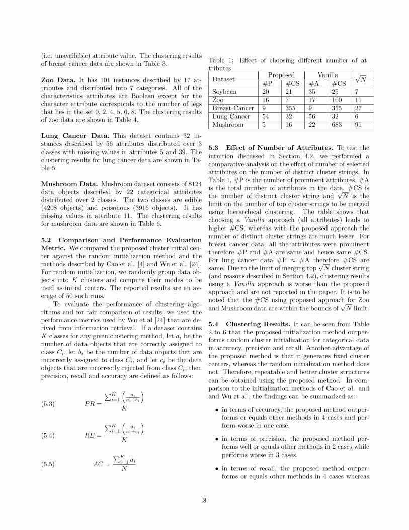
Table 1: Effect of choosing different number of at-tributes.

DatasetProposed Vanilla √

N#P #CS #A #CS

Soybean 20 21 35 25 7Zoo 16 7 17 100 11Breast-Cancer 9 355 9 355 27Lung-Cancer 54 32 56 32 6Mushroom 5 16 22 683 91

5.3 Effect of Number of Attributes. To test theintuition discussed in Section 4.2, we performed acomparative analysis on the effect of number of selectedattributes on the number of distinct cluster strings. InTable 1, #P is the number of prominent attributes, #Ais the total number of attributes in the data, #CS isthe number of distinct cluster string and

√N is the

limit on the number of top cluster strings to be mergedusing hierarchical clustering. The table shows thatchoosing a Vanilla approach (all attributes) leads tohigher #CS, whereas with the proposed approach thenumber of distinct cluster strings are much lesser. Forbreast cancer data, all the attributes were prominenttherefore #P and #A are same and hence same #CS.For lung cancer data #P ≈ #A therefore #CS aresame. Due to the limit of merging top

√N cluster string

(and reasons described in Section 4.2), clustering resultsusing a Vanilla approach is worse than the proposedapproach and are not reported in the paper. It is to benoted that the #CS using proposed approach for Zooand Mushroom data are within the bounds of

√N limit.

5.4 Clustering Results. It can be seen from Table2 to 6 that the proposed initialization method outper-forms random cluster initialization for categorical datain accuracy, precision and recall. Another advantage ofthe proposed method is that it generates fixed clustercenters, whereas the random initialization method doesnot. Therefore, repeatable and better cluster structurescan be obtained using the proposed method. In com-parison to the initialization methods of Cao et al. andand Wu et al., the findings can be summarized as:

• in terms of accuracy, the proposed method outper-forms or equals other methods in 4 cases and per-form worse in one case.

• in terms of precision, the proposed method per-forms well or equals other methods in 2 cases whileperforms worse in 3 cases.

• in terms of recall, the proposed method outper-forms or equals other methods in 4 cases whereas

8

it perform worse in 1 case.

Table 2: Clustering results for Soybean dataRandom Wu Cao Proposed

AC 0.8644 1 1 0.9574PR 0.8999 1 1 0.9583RE 0.8342 1 1 0.9705

Table 3: Clustering results for Breast Cancer dataRandom Wu Cao Proposed

AC 0.8364 0.9113 0.9113 0.9127PR 0.8699 0.9292 0.9292 0.9292RE 0.7743 0.8773 0.8773 0.8783

Table 4: Clustering results for Zoo dataRandom Wu Cao Proposed

AC 0.8356 0.8812 0.8812 0.891PR 0.8072 0.8702 0.8702 0.7302RE 0.6012 0.6714 0.6714 0.8001

Table 5: Clustering results for Lung Cancer dataRandom Wu Cao Proposed

AC 0.5210 0.5 0.5 0.5PR 0.5766 0.5584 0.5584 0.6444RE 0.5123 0.5014 0.5014 0.5168

Table 6: Clustering results for Mushroom dataRandom Wu Cao Proposed

AC 0.7231 0.8754 0.8754 0.8815PR 0.7614 0.9019 0.9019 0.8975RE 0.7174 0.8709 0.8709 0.8780

The above results are very encouraging due to thefact that the worst case time complexity of the proposedmethod is log-linear, whereas the method of Cao etal. has quadratic complexity and the method of Wuet al. induces random selection of data points. Theaccuracy values of proposed method are mostly betterthan or equal to other methods, which implies that theproposed approach is able to find fixed initial centersthat are close to the actual centers of the data. Theonly case where the proposed method perform worsein all three performance metric is the soybean dataset.We observe that on some datasets the proposed methodgives worse values for precision, which implies that

in those cases some data objects from non-classes aregetting clustered in given classes. The recall valuesof proposed method are mostly better than the othermethods, which suggests that the proposed approachtightly controls the data objects from given classes tobe not clustered to non-classes. Breast cancer datahas no prominent attribute in the data and uses allthe attributes and produces comparable results to othermethods. Lung cancer data, though smaller in sizehas high dimension and the proposed method is ableto produce better precision and recall rates than othermethods. It is also observed that the proposed methodperform well on large dataset such as mushroom datawith more than 8000 data objects. In our experiment,we did not get a scenario where the distinct clusterstrings are less than the desired number of clusters. Theproposed algorithm is also independent of the order ofpresentation of data due to he way mode is computedfor different attributes.

6 Conclusions

The results attained by the K-modes algorithm forclustering categorical data depends intrinsically on thechoice of random initial cluster center, that can causenon-repeatable clustering results and produce impropercluster structures. In this paper, we propose an algo-rithm to compute initial cluster center for categoricaldata by performing multiple clustering on attribute val-ues of attributes present in the data. The present algo-rithm is developed based on the experimental fact thatsimilar data objects form the core of the clusters andare not affected by the selection of initial cluster cen-ters, and that individual attribute also provide useful in-formation in generating cluster structures, that eventu-ally leads to computing initial centers. In the first pass,the algorithm produces distinct distinguishable clusters,that may be greater than, equal to or less than the de-sired number of clusters ( K ). If it is greater than K thenhierarchical clustering is used to merge similar clusterstrings into K clusters, if it is equal to K then dataobjects corresponding to cluster strings can be directlyused as initial cluster centers. An obscure possibilityarises when cluster strings are less than K, in whichcase either the value of K is to be reduced, or assumedthat the current value of K is not true representative ofthe desired number of clusters. However, in our exper-iment we did not get such situation, largely because itcan happen in a rare occurence when all the attributevalues of different attributes cluster the data in the sameway. These initial cluster centers when used as seed toK-modes clustering algorithm, improves the accuracy ofthe traditional K-modes clustering algorithm that usesrandom modes as starting point. Since there is a def-

9

inite choice of initial modes (zero standard deviation),consistent and repetitive clustering results can be gen-erated. The proposed method also does not depend onthe way data is ordered. The performance of the pro-posed method is better than or equal to the other twomethods on all datasets except one case. The biggestadvantage of the proposed method is the worst case log-linear time complexity of computation and fixed choiceof initial cluster centers, whereas both the other twomethods lack either one of them.

In scenarios when the desired number of clustersare not available at hand, we would like to extend theproposed multi-clustering approach for categorical datafor finding out the natural number of clusters presentin the data in addition to computing the initial clustercenters for such case.

References

[1] Michael R. Anderberg. Cluster analysis for applica-tions. Academic Press, New York, 1973.

[2] Daniel Boley, Maria Gini, Robert Gross, Eui-Hong Han, George Karypis, Vipin Kumar, BamshadMobasher, Jerome Moore, and Kyle Hastings.Partitioning-based clustering for web document cat-egorization. Decision Support Systems., 27:329–341,December 1999.

[3] Paul S. Bradley and Usama M. Fayyad. Refining initialpoints for k-means clustering. In Jude W. Shavlik,editor, ICML, pages 91–99. Morgan Kaufmann, 1998.

[4] Fuyuan Cao, Jiye Liang, and Liang Bai. A new initial-ization method for categorical data clustering. ExpertSystems and Applications, 36:10223–10228, 2009.

[5] A. Frank and A. Asuncion. UCI machine learningrepository, 2010.

[6] Ana L. N. Fred and Anil K. Jain. Data clustering usingevidence accumulation. In ICPR (4), pages 276–280,2002.

[7] K. Chidananda Gowda and E. Diday. Symbolic cluster-ing using a new dissimilarity measure. Pattern Recogn.,24:567–578, April 1991.

[8] Sudipto Guha, Rajeev Rastogi, and Kyuseok Shim.Rock: A robust clustering algorithm for categoricalattributes. In Proceedings of the 15th InternationalConference on Data Engineering, 23-26 March 1999,Sydney, Austrialia, pages 512–521. IEEE ComputerSociety, 1999.

[9] M. Hall, E. Frank, G. Holmes, B. Pfahringer, P. Reute-mann, and I. H. Witten. The weka data mining soft-ware: An update. In in SIGKDD Explorations, vol-ume 11 of 1, 2009.

[10] Zengyou He. Farthest-point heuristic based ini-tialization methods for k-modes clustering. CoRR,abs/cs/0610043, 2006.

[11] Zengyou He, Xiaofei Xu, and Shengchun Deng. A clus-

ter ensemble method for clustering categorical data.Information Fusion, 6(2):143–151, 2005.

[12] Zhexue Huang. A fast clustering algorithm to clus-ter very large categorical data sets in data mining. InResearch Issues on Data Mining and Knowledge Dis-covery, 1997.

[13] Zhexue Huang. Extensions to the k-means algorithmfor clustering large data sets with categorical values.Data Min. Knowl. Discov., 2(3):283–304, 1998.

[14] Anil K. Jain and Richard C. Dubes. Algorithms forclustering data. Prentice-Hall, Inc., Upper SaddleRiver, NJ, USA, 1988.

[15] L. Kaufman and P. J. Rousseeuw. Finding Groupsin Data: An Introduction to Cluster Analysis. JohnWiley, 1990.

[16] Shehroz S. Khan and Amir Ahmad. Computing initialpoints using density based multiscale data condensa-tion for clustering categorical data. In Proc. of 2ndInt’l Conf. on Applied Artificial Intelligence, 2003.

[17] Shehroz S. Khan and Amir Ahmad. Cluster centerinitialization algorithm for k-means clustering. PatternRecognition Letters, 25:1293–1302, 2004.

[18] Shehroz S. Khan and Shri Kant. Computation ofinitial modes for k-modes clustering algorithm usingevidence accumulation. In Proceedings of the 20thinternational joint conference on Artificial intelligence(IJCAI), pages 2784–2789, 2007.

[19] Jiri Matas and Josef Kittler. Spatial and feature spaceclustering: Applications in image analysis. In CAIP,pages 162–173, 1995.

[20] Pabitra Mitra, C. A. Murthy, and Sankar K. Pal.Density-based multiscale data condensation. IEEETransactions on Pattern Analysis and Machine Intel-ligence, 24(6):734–747, 2002.

[21] Euripides G. M. Petrakis and Christos Faloutsos.Similarity searching in medical image databases.IEEE Transactions on Knowledge Data Engineering.,9(3):435–447, 1997.

[22] H. Ralambondrainy. A conceptual version of thek-means algorithm. Pattern Recognition Letters,16(11):1147–1157, 1995.

[23] Ying Sun, Qiuming Zhu, and Zhengxin Chen. Aniterative initial-points refinement algorithm for cate-gorical data clustering. Pattern Recognition Letters,23(7):875–884, 2002.

[24] Shu Wu, Qingshan Jiang, and Joshua Zhexue Huang.A new initialization method for clustering categoricaldata. In Proceedings of the 11th Pacific-Asia confer-ence on Advances in knowledge discovery and data min-ing, PAKDD’07, pages 972–980, Berlin, Heidelberg,2007. Springer-Verlag.

10

Co-RCA: Unsupervised Distance-Learning for Multi-View Clustering

Matthias Schubert Hans-Peter KriegelInstitute for Computer Science Ludwig Maximilians University Munich

Oettingenstr. 67, D-80538 Munich{ schubert, kriegel}@dbs.ifi.lmu.de

Abstract

There has been a considerable effort on tuning distancemetrics for supervised problems such as kNN classifi-cation. Most methods in metric learning aim at deriv-ing an optimized matrix for the Mahanalobis distance.However, these methods cannot be applied for cluster-ing methods because there is no training set indicatingwhich instances are similar and which are not. In thispaper, we will show that the lack of training data canbe overcome by using multiple views. Our new methodCo-RCA combines the idea of co-learning with relevantcomponent analysis (RCA). Based on the assumptionthat the closest pairs in any useful feature space are se-mantically similar as well, it is possible to improve dis-tance measures in unsupervised learning tasks such asclustering. Our experiments demonstrate that Co-RCAcan improve the semantic meaning of the distances fortwo image data sets.

1 Introduction

One of the most essential aspects in developing success-ful knowledge discovery processes is finding suitable fea-tures spaces. In a well-suited feature space the distancebetween two objects should reflect the semantic simi-larity holding in the given application. There are basi-cally two methods of optimizing a feature space to bet-ter represent the underlying similarity structure. Thefirst method is to directly manipulate the feature space,for example removing redundant and unimportant fea-tures or deriving new features. The second method ismanipulating the employed comparison function whichis used to compute object similarity. In most cases,the comparison function is either a kernel function ora distance metric. The most common framework foroptimizing features spaces are affine transformations,like principal component analysis (PCA) and its exten-sions. The most common framework for metric learningis the Mahalanobis distance or quadratic form which isbased on a matrix modeling how the features are corre-lated. It can be shown that any matrix that guarantees

that the Mahalanobis distance is a metric correspondsto a linear basis transformation where the Euclidian dis-tance in the transformed space is equivalent the Maha-lanobis distance in the original space. There exists awide variety of methods for learning a proper Maha-lanobis distance or the equivalent transformation ma-trix for supervised problems [18]. The core idea of anysuch method is to decrease the distances between sim-ilar objects while increasing the distances between dis-similar objects. To construct an optimization problem,metric learning methods employ examples to measurethe contrast between the similarity being computed inthe features space and the similarity being observed bya human expert. For classification, information aboutsimilarity is usually drawn from the class labels. Objectsbelonging to the same class are considered to be similarand objects belonging to different classes are consideredto be dissimilar. Requiring that all objects belongingto the same class are closer to each other than to anyobject of any different class is often a too strict goal.Therefore, many methods relax this requirement. Forexample, it might be sufficient to optimize the similar-ity to the k-closest neighbors from the same class insteadof the similarity to all other members of the same class.Though there are many successful methods for metriclearning for supervised tasks, optimizing feature spaceswithout examples for similar and dissimilar objects re-ceived less attention by researchers. Though there aremany methods which try to reduce the dimensionalityof feature spaces such as PCA, the positive effect onthe quality of the feature space is mainly achieved byremoving redundant information and rescaling the re-maining features. In some cases, the observed varianceof the resulting feature values gives hints on the impor-tance of a feature. However, a large variance can becaused by a feature which is generally measured by alarger scale. Thus, the feature does not need to havean increased importance. To conclude, though meth-ods like PCA yield a powerful tool for improving dataquality, the available information is often not enough to

11

improve the meaning of the observed distances.In this paper, we consider the case of data which is

represented in multiple feature spaces also called multi-view or multi-represented data. The core idea of ourapproach is to improve the similarity information in afeature space by employing the similarity informationdrawn from other views. Thus, the method is unsu-pervised but integrates information about object simi-larity which is not derived from the particular featurespace that is currently optimized. Technically, our ap-proach is based on the idea of ensemble learning andco-training in particular. Therefore, there are two im-portant requirements to the underlying feature spaces.The first is that the information about object similar-ity provided by different views should be sufficientlyindependent from each other. For example, using tex-ture and color features should yield independent featurespaces because each of the feature spaces is based on adifferent characteristic of a pixel image. The second re-quirement of ensemble learning is that each weak learneris sufficiently accurate. In our setting it is required thatthere must be a sufficiently large number of cases wherea small distance corresponds to a large similarity andlarge distance corresponds to a small degree of simi-larity. Our algorithm Co-RCA is derived from the co-training framework introduced in [4]. In a first step, wederive examples indicating similarity or dissimilarity fora smaller number of object comparisons from an initialfeature representation. In particular, we consider thek-closest pairs and k-farthest pairs of objects and usethem to determine similar and dissimilar object pairs.Given these examples, we employ relevant componentanalysis(RCA) to improve the structure of the next fea-ture space. Thus, the set of examples for similar anddissimilar objects is increased with each iteration. Thealgorithm terminates when no new example pairs forsimilar objects are retrieved from either feature space.Thus, the k-closest pair in all views are stable under thecurrent transformation.

The rest of the paper is organized as follows: Insection 2, we review related work on metric learningand feature reduction. Section 3 will shortly surveythe two techniques our method is based on, co-trainingand RCA. The new algorithm Co-RCA is introduced insection 4. The results of our experimental evaluationare described in section 5. The paper concludes with abrief summary in section 6.

2 Related Work

In this section, we briefly review existing approachesto metric learning and affine optimizations of vectorspaces.

Most distance learning try to optimize the Maha-

lanobis distance. In the following, we give a short sum-mary of existing metric learning approaches. A de-tailed survey can be found in [18]. Among super-vised approaches one of the first methods is Fisher’sLinear Discriminant (FLD) [10]. It maximizes the ra-tio of the between-class variance and the within-classvariance using a generalized eigenvalue decomposition.This method has been extended by Belhumeur et al. [2]to the Fisherfaces approach. It precedes FLD with areduction of the input space to its principal compo-nents and can thus filter unreliable input dimensions.With RCA [1], Bar-Hillel et al. focus on the problemof minimizing within-chunklet variance. They arguethat between-class differences are less informative thanwithin-class differences and that class assignments fre-quently occur in such a way that only pairs of equally-labelled objects can be extracted. These pairs are ex-tended into chunklets (sets) of equivalent objects. Theinverse chunklet covariance matrix is used for calculat-ing the Mahalanobis distance. NCA [11] proposed byGoldberger et al. optimizes an objective function basedon a soft neighborhood assignment evaluated via theleave-one-out error. This setting makes it more resistantagainst multi-modal distributions. The loss functionis differentiated and then optimized by general gradi-ent descent approaches like delta-bar-delta or conjugategradients. The result of this optimization is a Maha-lanobis distance directly aimed at improving nearest-neighbor classification. The objective function is, how-ever, not guaranteed to be convex. With Information-Theoretic Metric Learning (ITML) [8], Davis et al. pro-pose a low-rank kernel learning problem which gener-ates a Mahalanobis matrix subject to an upper boundfor inner-class distances and a lower bound to between-class distances. They regularize by choosing the matrixclosest to the identity matrix and introduce a way toreduce the rank of the learning problem. LMNN (LargeMargin Nearest Neighbor) [16] by Weinberger et al. isbased on a semi-definite program for directly learninga Mahalanobis matrix M . They require k-target neigh-bors for each input object x, specifying a list of objects,usually of the same class as x, which should always bemapped closer to x than any object belonging to anyother class. These k-target neighbors are the within-class k-nearest neighbors. Hence, the loss function con-sists of two terms for all data points x. One penalizingthe distance of x to its k-target neighbors and a secondpenalizing close objects being closer to x than any of itstarget neighbors.LMNN requires a specialized solver inorder to be run on larger data sets. For multi-view met-ric learning, there are already some methods for semi-supervised settings [17, 19]. Though these methods doexploit multiple views as Co-RCA does, they still re-

12

quire label information even if the amount of labels isexpected to be limited.

The main idea of unsupervised approaches is to re-duce the feature space to a lower-dimensional space inorder to eliminate noise and enable a more efficientobject comparison. The criteria for selecting such asubspace are manifold. Principal Component Analysis(PCA) [12], builds an orthogonal basis aimed at bestpreserving the data’s variance, Multidimensional Scal-ing (MDS) [7] seeks the transformation which best pre-serves the geodesic distances and Independent Compo-nent Analysis (ICA) [6] targets a subspace that guar-antees maximal statistical independence. ISOMAP [15]by Tenenbaum et al. is a non-linear enhancement of theMDS principle, in identifying the geodesic manifold ofthe data and preserving its intrinsic geometry. Otherunsupervised approaches (e.g. [14, 3]) try to fulfill theabove criteria on a local scale.

3 Preliminaries

Co-Training The co-training framework was in-troduced by Blum and Mitchell and in [4]. In partic-ular their original work aimed at the improvement ofwebpage classification under the condition of a limitedset of labeled training data. The original set of exper-iments used two views on webpages. The first view istext vectors being derived from the actual content ofthe webpage. The second view consists of the anchortexts of the hyper links being directed at the webpage.Let us note that both views are sufficiently independentbecause the words in the anchor text need not appear inthe actual content as well. When starting the algorithmthere is a large set of web pages being described by bothviews. However, only a limited portion of the pages arelabeled w.r.t. the given classification task. The algo-rithm starts with training a text classifier on the firstview based on the already labeled pages. Let us notethat the resulting classifier must meet a sufficiently largeaccuracy to act as a weak classifier because co-trainingis in its essence an ensemble learning approach. Giventhe first classifier the method samples a set of unlabeledwebpages and uses the classifier to predict class labelsfor these pages. In the next step, the algorithm joins thenewly labeled objects with the already labeled objectsinto a new training set and switches the views. Thus, inthe next step a second classifier is trained based on theextended set of training objects. Since the second clas-sifier is based on a different view of the data, it modelsthe classes independently even though its training set ispartly made of automatically labeled example vectors.Again the classifier is used to extend the training set.Afterwards the algorithm switches to the next view andproceeds in the same way. The algorithm is stopped

when a predefined number of iterations is computed.Though the general process of Co-RCA and co-

training have a similar algorithmic scheme, there areconsiderable differences. First of all, co-training isaimed at the supervised task of classification with lim-ited label information. Co-RCA offers a method to im-prove the expressiveness w.r.t. multiple views withoutany task specific labeling. Thus, Co-RCA does not re-quire any labels but is leveraged by the assumption thatthe closest and most distant object pairs in a view arereally similar or dissimilar respectively.

Fisher Faces and RCA Fisher Faces [2] are anextension of the well known linear classifier known asFisher’s discriminant analysis (FDA). The core ideaof FDA is to compare feature correlations occurringbetween objects of the same class to those occurringbetween objects belonging to different classes. Thus,the method needs to derive two covariance matrices:The within class matrix Mw and the between classmatrix Mb. To determine Mw a covariance matrix foreach class c Mc is build and afterwards summed upover all classes C : Mw =

∑c∈CMc

Mb is computed as the covariance matrix of the classmeans µc for each class c ∈ C.

The idea of FDA is now to find dimensions thatmaximize the ratio of the covariance between classeswhile considering the covariances within the classes.Thus, FDA searches the direction ~w which maximizesthe target function S in the following equation:

S(~w) =~wT ·Mb · ~w~wT ·Mw · ~w

S can be reduced to a generalized eigenvalue problemand thus, the optimal ~w is the eigenvector correspond-ing to the largest eigenvalue of M−1w ·Mb. Using ~w as thenormal vector of a hyperplane yields a linear classifier.However, when considering the complete base of eigen-vectors and weighting them with their inverse eigenval-ues yields an affine transformation of the feature space.In the transformed feature space the distances can beexpected to express similarity w.r.t. the class labels ina much better way. Let us note that though there aremore recent and accurate approaches to supervised met-ric learning, Fisher Faces are still rather popular due totheir simplicity.

Relevant Component Analysis (RCA) was intro-duced in [1] and overcomes several problems of Fisherfaces. A first problem of Fisher faces is that it cannotbe guaranteed that Mw is invertible. Therefore, RCAintroduces an PCA step to eliminate linear dependen-cies. Another difference is that RCA does not directlyoptimize the feature space to separate classes. Instead

13

of objects labeled with classes, RCA requires sets of sim-ilar objects called chunks. Therefore, the authors intro-duce RCA as an unsupervised method. In this paper, weconsider RCA as a supervised method because it still re-quires examples in the form of chunks. For each chunk,the covariance matrix is built and summed up into amatrix corresponding to Mw. Determining the counter-part to Mb in FDA yields another problem. Thoughwe have the information that vectors within the samechunk are similar, we cannot conclude that vectors fromdifferent chunks are dissimilar. Therefore, to model thecovariance w.r.t. dissimilar objects, RCA considers thecovariance matrix Mall w.r.t. any object of the data set.The idea behind this solution is the following. For anyobject o in the data set DB, the majority of objects isusually quite dissimilar. Thus, Mall resembles the co-variances of dissimilar objects to a much larger extendthan those being observed for similar objects.

Though the optimization step of RCA is quitesimilar to the optimization step in Co-RCA, thereis some important differences. While RCA assumesgiven information about sets of similar objects (chunks),our algorithm does not require any such information.Instead the information that is required for determiningMw is completely derived from other views by co-learning. Another difference is that Co-RCA works ona sample of object pairs being represented as differencevectors. Thus, the covariance information is not relatedto a mean value but over any distance computationin the complete feature space. Finally, while RCAsuffices to compute Mall to represent the covariance fordissimilar objects, Co-RCA maintains a dedicated set ofexample comparisons for dissimilar object pairs.

4 Co-RCA

A multi-view object o is given by an n-tuple(x1, . . . , xn) ∈ Fi × . . . × Fn of feature vectors drawnfrom various feature spaces Fi. Each feature spaceFi is a subset of Rdi having the dimensionality ofdi ∈ N. In the following, we will also refer to Fi asthe ith view. To measure the similarity between twovectors in view Fi, we assume the Euclidian distance:dist(xi, yi) = ‖xi − yi‖

Our goal is now to find an affine transformationBi for improving Fi in a way that dist(xi · Bi, yi · Bi)yields a better approximation for the similarity of ox, oythan dist(xi, yi). In particular, we want to decrease thedistances of similar objects and increase the distancesbetween dissimilar objects. To achieve this goal, we relyon the same optimization as FDA and RCA:

S(~w) =~wT ·Mdis · ~w~wT ·Msim · ~w

A major difference of Co-RCA to ordinary RCAare the covariance matrices Mdis and Msim whichare determined in a different way from the previouslydiscussed methods.

To estimate both matrices, we assume two examplesets. The first set Tsim consists of multi-view objectpairs (o, u) being similar and the second set Tdis consistsof examples for pairs of dissimilar objects. Note that thesets consists of complete multi-view objects and not offeature vectors because similarity is considered to holdfor the complete object without any restriction to aparticular view. Given an example set of pairs of multi-view objects, we can now determine the covariancematrices M i

sim and M idis in the ith view Fi. Since

a covariance matrix is built from feature vectors andnot from object pairs, we first of all built the differencevector for each object pair o, u with o = (x1, .., xn),u =(y1, .., yn) in view Fi: δi(o, u) = xi − yi. However, sincethe order of o, u in an object pair is arbitrary and theorder of vectors for determining δi(o, u) is not, we alsohave to consider the inverse vector δi(u, o) = yi − xi.Thus, we have to derive a set of 2k difference vectorsfrom an example set of k object pairs.

Using distance vectors to optimize a feature spacehas a major impact to the method. A first effect is thatresulting data distribution is always point symmetric tothe origin. Thus, describing the distribution by a co-variance matrix makes sense in most cases. Anotherimportant consequence is the amount of distance vec-tors has the quadratic size of the data set. Thus, itis often required to restrict the optimization to samplesets instead of computing the distribution of the com-plete set of distance vectors. A final result of usingdifference vectors is that the optimization is indepen-dent from the any locality within the data set. Thus,the information about locations of the compared ob-jects within the feature space is completely discardedand only the information about the relative position-ing of both objects is preserved. Since the goal of ourmethod is to find a global affine transformation for thecomplete feature space, our model cannot cope with lo-cal differences in the meaning of the features anyway.Additionally, unlike FDA and RCA, we do not have tomake any assumption of the locality of similar objects.Thus, we do not need a compact area in the data spacewhere all objects are considered to be similar to eachother such as chunks or classes.

Formally, we can derive M isim for the example set

Tsim in the following way:

M isim(Tsim) =∑

(o,u)∈Tsimδi(o, u) · δi(o, u)T + δi(u, o) · δ(u, o)T

2 ∗ |Tsim|

14

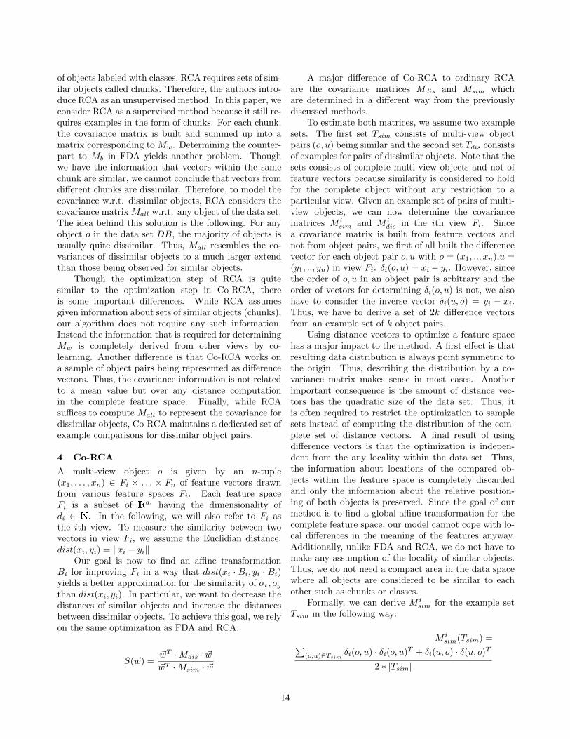
Figure 1: Feature space with depicted closest pairs and farthest pairs(left). Corresponding distribution of distancevectors (right).

M idis is determined in the same way by exchanging

Tsim with Tdis.Now that we know how to determine the matrices

based on object pairs, we have to find a way tofind meaningful example sets for similar and dissimilarobjects. The solution in this paper is based on thefollowing assumption: If two objects have a very smalldistance in a feature space that is useful for describingsimilarity, it is very likely that they are semanticallysimilar as well. To find pairs of semantically dissimilarobjects, we can use a similar argumentation: If twoobjects are very different in some feature space, it isvery likely that they are really dissimilar to each otherw.r.t. the judgement of a human expert. Let us notethat the sets of k-closest and k-farthest object pairsdo not necessarily contain information about all dataobjects in the data set. It is very likely that the samplesets contain multiple object pairs containing featurevectors being located in more dense areas. A furtherimportant aspect of our method is that the closestobject pairs in one feature space are used to optimize thenext dimension. Thus, the object pairs being collectedin view Fi are used to derive difference vectors inview Fi+i where the corresponding distances might beconsiderably larger. Let us note that the major reasonthis assumption holds in most cases is that domainexperts tend to select meaningful representations whichare already selected because they are connected to thetask at hand. An expert would not select color featuresfor comparing medical images such as x-Ray or CTimages, but grey values, gradients and textures. Thus,using views that do not measure aspects of importanceto object similarity will lead Co-RCA to model anunwanted notion of similarity. An illustration for ourmethod to determine covariance matrixes is depictedin figure 1. In the left picture, there is a set withsome object pairs being marked as similar(dashed lines)

and some object pairs being dissimilar (solid lines). Inthe right picture, we see the corresponding differencevectors and surrounding ellipses for each distributionsto show the general correlations. Though we only havesome information given by object pairs, the distributionfor similar and dissimilar objects offers a good model toseparate the red from the blue vectors on the left side.

To summarize, the example set Tsim is extended inthe ith view of the data set DB by calculating the k-closest pairs in view i. Analogously, we can record thek pairs of feature vectors having the largest pairwisedistance in view i to gather examples for Tdis.

The Co-RCA algorithm requires a set of multi-viewdata objects DB and a sample size k as input. Thenumber of views n needs to be at least two.The outputof our algorithm is a set a affine transformation Bi foreach view Fi that minimizes the distances of the objectpairs in Tsim compared to the dissimilar object pairsin Tdis. Since the transformation for each view tries tomirror the same set of similarity relations, Co-RCA triesto achieve an agreement of views.

The algorithm starts with determining Tsim andTdis from the k-closest and k-farthest pairs in the firstview F0. Then the algorithm enters its main loop wherea transformation for the next view F1 is computedand new elements are added to Tsim and Tdis. Thealgorithm terminates when no additional examples canbe found among the k closet pairs in any view. Wewill now explain the steps that are performed in eachiteration in greater detail. We start with switchingto the next view. When reaching the last view, wereturn to the first one. To derive the sample sets ofdifference vectors in the current view, we have to iterateover Tsim. For each object pair (o, u) ∈ Tsim, wehave to compute the difference vector δi(o, u) and useit compute M i

sim. Correspondingly, we iterate over Tdisand calculate M i

dis. Let us note that it is important

15

Co‐RCA ( MR_Database DB, k)rep := 1nochange := 0T_sim := k‐closet‐pairs(DB[rep],k)T di k f h i (DB[ ] k)T_dis := k‐farthest‐pairs(DB[rep],k)B[] //result transformation for all repswhile( |T_sim|+| T_dis| > old or nochange ≠ n)

rep (rep +1)mod nrep := (rep +1)mod nM_sim := Covariance(T_Sim, rep)M_dis := Covariance(T_dis rep)B[rep] :=RCA (M sim M dis DB[rep])B[rep] :=RCA (M_sim , M_dis,DB[rep])newDB := RCA[rep](DB[rep])T_sim := T_sim∪ k‐closet‐pairs(newDB,k)T dis := T dis∪ k‐farthest‐pairs(newDB k)T_dis := T_dis∪ k farthest pairs(newDB,k)if |T_sim|+| T_dis| = old

nochange := nochange+1elseelse

nochange := 0endifold:=|T_sim|+| T_dis| | _ | | _ |

endwhilereturn B[]

Figure 2: Pseudocode of Co-RCA for n views.

that Tsim and Tdis contain examples being close inother views but not in Fi. Thus, Fi is optimized tocontain similarity relationships from the other views.Then, we employ both matrices in the optimizationstep being similar to RCA. The result is an affinetransformation Bi. The step starts with performingan PCA on M i

sim to make sure it is invertible. Afterapplying the PCA, we solve the eigenvalue problem on(M i

sim)−1 ·Mdis. The resulting affine transformation Biis composed of the weighted eigenvectors of (M i

sim)−1 ·Mdis where each eigenvector vj is weighted with theinverse square root of the corresponding eigenvalueλj :

1√√λj

. This transformation is also known as

whitening transformation. The transformation Bi isnow applied to the the view Fi. Then, the k-closestand the k-farthest pairs of object are determined in thetransformed feature space leading to new example sets

`Tsim and `Tsim which are joined to the already knownexample sets Tsim and Tdis. Let us not that it is possiblethat `Tsim ⊂ Tsim or `Tdis ⊂ Tdis, indicating that theview is already consistent with the example sets. Thealgorithm stops when all views are consistent with theexample sets, i.e. no new examples can be found toextend the example pairs. Therefore, it is necessarythat there are n consecutive iterations not adding anynew examples. The pseudo code of Co-RCA is depictedin figure 2.

So far the result of Co-RCA is an affine transfor-mation Bi for each feature space Fi. However, in orderto employ the results in data mining, it is necessaryto integrate the transformations into the data miningalgorithm. The simplest way to do this is to add the

feature transformations Bi into the preprocessing stepof the knowledge discovery process and only work withthe transformed feature spaces. Another option is to usethe original features spaces and work with Mahanalobisdistance using BTi ·Bi. A further problem is how to em-ploy all representations for determining similarity. Thesimplest solution to do this would be to employ onlya single representation. Since the similarity statementsshould agree, similarity should be reflected in all repre-sentations in a similar way. However, though Co-RCAcan improve the similarity relationships in the partic-ular representation, a less useful relation might not betransformed into a very useful one by means of a affinebasis transformation. Thus, it is very likely that somerepresentations yield more information than others andusing a single representation yields the risk of selectinga less informative one. We therefore argue to employ allrepresentations by means of a simple multi-representeddistance measure such as the normalized sum of dis-tances:

distnorm(o, u) =

n∑

1=i

wi · ‖xi − yi‖

where wi is a weight factor reflecting the importance ofrepresentation i. If no weight is available all represen-tations can be weighted equally, setting wi = 1. Havinga multi-view distance measure allows us to use multi-ple distance-based data mining algorithms like density-based clustering such as DBSCAN [9]. Furthermore, theresulting affine transformations can be easily integratedinto multi-view kernel learning.

5 Experimental Evaluation

In this section, we present the results of preliminaryexperiments with Co-RCA. We test our method ontwo image data sets where each image is categorizedinto exactly one class. The first data set (Conf183)contains 183 pictures belonging to 35 classes which werephotographed during two sightseeing trips. The seconddata set S4B consists of 1743 photographs from 80classes. We extracted color moments, texture features[13] and facet-orientations [5] for each image in bothdata sets. Thus, both experiments were done on 3representations.

As comparison partner, we chose the original fea-tures spaces and their linear combination. Furthermore,we wanted to compare Co-RCA to the closest supervisedmethod which is RCA. As chunks for training RCA, weemployed the class label. The classes in both data setshave all a limited amount of instances and thus, they arewell-suited to be used as chunks. We employed RCA tosee how closely the result of the unsupervised Co-RCAwould get to a supervised method. The sample size k for

16

1 0

0.9

1.0

0.7

0.8

0

0.6

0.7uracy

0.4

0.5

Accu

0.2

0.3Original

C RCA

0 0

0.1

0.2 Co‐RCARCA

0.0

texture color moments facet all

(a) Conf 183

0 7

0 6

0.7OriginalCo‐RCA

0.5

0.6RCA

0.4

racy

0.3Accur

0.2

0 0

0.1

0.0

texture color moments facet all

(b) S4B

Figure 3: 1NN classification accuracies being achieved on each representation and their linear combination.

Co-RCA was set to 250 for the smaller data set conf183and to 5000 for the larger data set S4B. Let us note thatthough these sample sizes seem to be rather large, theyare still comparably small to the number of all possi-ble difference vectors. All methods were implementedin Java 1.7 and tests were run on a dual core (3.0 Ghz)workstation with 2 GB main memory.

A first test for the quality of a feature space isnearest neighbor classification. In other words, we testin how many cases the closest neighbor in a given datarepresentations is from the same class as the queryobject. To avoid that the query object is part of thedatabase itself, we tested using stratified 10-fold cross-validation. Let us note that we trained RCA and Co-RCA on the complete data set instead of the limitedtraining set within each fold. This, approach is viablefor Co-RCA because it is a completely an unsupervisedmethod. For RCA, the results might slightly overfit.However, since RCA is only a comparison partner tothe unsupervised Co-RCA, the results are sufficientto show how close Co-RCA might get to RCA. Theresults are shown in figure 3. For the small andrelatively easy conf183 data set. The 1NN classifieron the original feature set without any optimizationachieved classification accuracies between 50 % and 70%. The combination off all three representations did notyield a performance advantage but performed similarto the best single representation, i.e. color moments.As expected the supervised RCA achieved the bestresults for all representations and the combination offall representations improved the accuracy by 4 %. Theunsupervised Co-RCA achieved between 2% and 5 %less classification accuracy than the supervised RCAfor all representations. For the best result achievedby combining all representations, the performance wasonly 2% less accurate than for the supervised method.The plot for the larger and more difficult S4B data set

shows similar results. The 1NN classification on theoriginal feature spaces did not yield convincing results.However, the unsupervised Co-RCA managed to getvery close to the supervised RCA. For the combinationof all three representations, Co-RCA achieved only 3 %less accuracy. To conclude, by exploiting the structureof 3 different views of the data set, it was possibleto considerably improve the similarity of the nearestneighbors in the underlying feature space.

In the next experiment, we measure the perfor-mance w.r.t. all similar objects in the data set andnot just for the closest ones. Thus, we pose a rankingquery for each data object and count the number of re-sult objects belonging to the same class. The resultingprecision recall graph is averaged over all possible queryobjects in the database and displays the number of truehits (precision) in the result set containing at least x %of the similar objects in the database (recall). For bothgraphs, we can observe a similar behavior. Though Co-RCA cannot achieve the high precision levels of RCA,it is still able to considerably improve the precision forany measured level of recall. For the more difficult dataset S4B, the graph is even considerably closer to thesupervised benchmark than to the default case of thelinear combination of the original feature spaces.

6 Conclusions

In this paper, we presented ongoing work in unsuper-vised feature space optimization for multi-view data.The core idea of our new method Co-RCA is to combineco-training and distance learning methods to generate amulti-view data space yielding a better model for objectsimilarity. The leverage of our unsupervised method isthe observation that very close and very distant objectsin a meaningful feature space usually indicate pairs ofobjects which are semantically similar or dissimilar aswell. Based on this type of information, it is possible

17

1

0.9

1

0.7

0.8

0.5

0.6cision

0.3

0.4Pre

Original

0.1

0.2OriginalCo‐RCARCA

0

0.1

0 25 0 45 0 65 0 850.25 0.45 0.65 0.85

Recall

(a) Conf 183

0.40

0.45

Original

0.30

0.35 Co‐RCA

RCA

0 20

0.25

0.30

cision

0.15

0.20

Pre

0.05

0.10

0.00

0.05

0 25 0 45 0 65 0 850.25 0.45 0.65 0.85

Recall

(b) S4B

Figure 4: Precision-recall graph for the joint representations for the three types of feature spaces.

to iteratively select examples for similar and dissimilarobject pairs from all representations. In a co-trainingalgorithm we iteratively optimize the feature spaces andselect new examples. Our experiments indicate that ournew algorithm Co-RCA can generate feature transfor-mations of almost comparable quality as the supervisedapproach our methods is built on, RCA.

References

[1] A. Bar-Hillel, T. Hertz, N. Shental, and D. Wein-shall. Learning distance functions using equivalencerelations. In Proceedings of the 20th InternationalConference on Machine Learning (ICML), Washing-ton, DC, USA, pages 11–18, 2003.

[2] P. N. Belhumeur, J. P. Hespanha, and D. J. Krieg-man. Eigenfaces vs. Fisherfaces: Recognition usingclass specific linear projection. IEEE Transactions onPattern Analysis and Machine Intelligence, 19(7):711–720, 1997.

[3] M. Belkin and P. Niyogi. Laplacian eigenmaps for di-mensionality reduction and data representation. Neu-ral Computation, 15(6):1373–1396, 2003.

[4] A. Blum and T. Mitchell. Combining labeled andunlabeled data with Co-training. In Proceedings of the11th Annual Conference on Computational LearningTheory (COLT), Madison, WI, pages 92–100, 1998.

[5] G. Chinga, O. Gregersen, and B. Dougherty. Pa-per surface characterisation by laser profilometry andimage analysis. Journal of Microscopy and Analysis,84:5–7, 2003.

[6] P. Comon. Independent component analysis, a newconcept? Signal Processing, 36(3):287–314, 1994.

[7] T. F. Cox and M. A. A. Cox. Multidimensional Scaling.Chapman & Hall/CRC, 2nd edition, 2001.

[8] J. Davis, B. Kulis, S. Sra, and I. Dhillon. Information-theoretic metric learning. In in NIPS 2006 Workshopon Learning to Compare Examples, 2007.

[9] M. Ester, H.-P. Kriegel, J. Sander, and X. Xu. Adensity-based algorithm for discovering clusters in large

spatial databases with noise. In Proceedings of the 2ndACM International Conference on Knowledge Discov-ery and Data Mining (KDD), Portland, OR, 1996.

[10] R. A. Fisher. The use of multiple measurements intaxonomic problems. Annals of Eugenics, 7:179–188,1936.

[11] J. Goldberger, S. Roweis, G. Hinton, and R. Salakhut-dinov. Neighborhood component analysis. In Advancesin Neural Information Processing Systems, pages 513–520. MIT Press, 2004.

[12] R. C. Gonzalez and R. E. Woods. Digital ImageProcessing. Addison-Wesley Longman Publishing Co.,Inc., Boston, MA, USA, 2001.

[13] R. M. Haralick, K. Shanmugam, and I. Dinstein. Tex-tural features for image classification. IEEE Transac-tions on Speech and Audio Processing, 3(6):6103–623,1973.

[14] S. T. Roweis and L. K. Saul. Nonlinear dimension-ality reduction by locally linear embedding. Science,290(5500):2323–2326, 2000.

[15] J. B. Tenenbaum, V. Silva, and J. C. Langford. Aglobal geometric framework for nonlinear dimensional-ity reduction. Science, 290(5500):2319–2323, 2000.

[16] K. Q. Weinberger, J. Blitzer, and L. K. Saul. Distancemetric learning for large margin nearest neighbor clas-sification. In Advances in Neural Information Process-ing Systems, Cambridge, MA, USA, 2006. MIT Press.

[17] B. Yan and C. Domeniconi. Subspace metric ensemblesfor semi-supervised clustering of high dimensional data.In Proceedings of the 10th European Conference onPrinciples of Knowledge Discovery and Data Mining(PKDD), Berlin, Germany, 2006.

[18] L. Yang. An overview of distance metric learning.Technical report, Department of Computer Science andEngineering, Michigan State University, 2007.

[19] D. Zhai, H. Chang, S. Shan, X. Chen, and W. Gao.Multi-view metric learning with global consistencyand local smoothness. In ACM Trans. on IntelligentSystems and Technology, 2011.

18

New Subspace Clustering Problems in the Smartphone Era

Dimitrios GunopulosUniversity of Athens

dg@di.uoa.gr

Vana KalogerakiAthens Univ. of Economics and Business

vana@aueb.gr

Abstract

We describe current and future work on the problemof subspace clustering and its application in the cur-rent environment where powerful, programmable mobilecommunication and computing devices proliferate. Weshow that a smartphone cloud computing infrastructureis feasible. We focus on specific variations of the sub-space clustering problem, namely the need to developalgorithms that take into account input from the userand the need for privacy preserving algorithms.

1 Introduction

The proliferation of powerful, programmable mobile de-vices along with the availability of wide-area connectiv-ity has provided a powerful platform to sense and sharelocation, motion, acoustic and visual data. People carrythese devices with them everywhere. In the early 2010period, it is reported that 42.7 million people in theU.S. alone own smartphones, 18 percent higher than 4months prior [1]. These devices are outfitted with awide array of sensing capabilities such as GPS, WiFi,microphones, cameras and accelerometers.

These mobile devices allow always on, full featuredconnectivity, and they bring a true revolution in theway people connect and use the web. We are nowentering an era where people can share aspects of theirlives online, creating virtual communities, and becomingboth data producers and data consumers at the sametime. With smartphones becoming the mobile platformof choice, a number of applications have emerged in awide variety of domains such as personal life, traveland work. Examples include traffic monitoring forreal-time delay estimation and congestion detection [2],location-based services such as personalized weatherinformation, locating areas of good WiFi connectivity,location-based games or receiving spatial alarms uponthe arrival to a reference time point [3], and socialnetworking applications for sharing photos and personaldata with family and friends [4].

The data collection capabilities that are embeddedin these mobile devices coupled with the fact that theirprocessing power, networking capability and resource

capacity is increasingly rapidly, has make these devices avery attractive and significant platform for smartphonecloud computing[5].

2 Desiderata for new mobile systems

Using smartphones to create a cloud computing infras-tructure opens up new opportunities for mobile com-puting. The exploitation of these capablities providesexcellent opportunities to sense data at locations wherepeople travel and provides many possible applicationsto study users’ behaviors [6] while the users themselvesprovide automatic mobility for sensors.

Although today’s mobile devices offer a powerfulsensing and a versatile computing platform, developingapplications to take advantage of them is challengingdue to a number of issues that must be addressed. Wehave established the following design considerations forthe development of the mobile systems and applicationsof the future:

1. Distributed Computation: The system shouldbe distributed, so that it scales with the number ofusers and does not have a single point of failure.

2. Ease of Development: The MapReduce frame-work has been successfully used to develop largescale distributed applications, and its use can sig-nificantly simplify and ease the programming anddeployment costs of distributed mobile systems inthe future.

3. Security and Privacy: The system should lever-age and promote user collaboration; however itshould safeguard the individual user resources andprotect the privacy of the individual user data.

4. Ease of Use: The application must be easy touse, so that a user can receive and understandthe results easily. This means that the solutionsmust be presented in an intuitive and easy tocomprehend way, but also that the user should havethe ability to tune the solutions based in his on herneeds, in a way as simple as possible.

5. Connectivity and failures: The problem of han-dling spotty connectivity and failures gracefully,which is a problem afflicting all mobile systems.

19

We note here, that some traditional considerationsof mobile distributed systems become less important inour setting. For example, devices such as smart-phonesand PDAs naturally use a lot of power and therefore aretypically charged regularly–daily. Power consumption,a very important problem in traditional sensor systems,while still important, is less important for such mobiledevices.

We should also emphasize here that one differencebetween a cloud of smartphones and the traditional ITinfrastructure is how privacy issues can be addressed;data does not have to be communicated and stored intoremote servers in a data center, data is rather keptprivately on the user phones and communicated onlywhen certain conditions arise or is needed by the user.Finally the cost model is different as well. The mobilecloud is an alternative to traditional data centers whereservers are usually dedicated to particular applications,as mobile clouds have low infrastructure costs, lowmanagement overhead and exhibit greater flexibility.

3 The MapReduce Framework

To fully take advantage of the available resources, asimple, but versatile system which eases developmentdeployment of software is essential. To this end wehave developed Misco [7], a system that implements aMapReduce framework targeted for smartphones andmobile devices. The MapReduce framework [8] is aflexible, distributed data processing framework designedto automatically parallelize the processing of long run-ning applications on petabyte sized data in clusteredenvironments. The MapReduce programming model [8]supports the weak connectivity model of computationsacross open networks, such as mobile networks, whichmakes it very appropriate for a mobile setting.

MapReduce provides two functional language prim-itives: map and reduce. The map function is ap-plied on a set of input data and produces intermedi-ary < key, value > pairs, these pairs are then groupedinto R partitions by applying some partitioning func-tion (e.g. hash(key) MOD R). All the pairs in thesame partition are passed into a reduce function whichproduces the final results.

The MapReduce programming model provides asimple way to split a large computation into a numberof smaller tasks; these tasks are independent of eachother and can be assigned on different worker nodes toprocess different pieces of the input data in parallel.

Application development is greatly simplified as theuser is only responsible for implementing the map andreduce functions and the MISCO system handles thescheduling, data flow, failures and parallel execution of

the applications.The Misco system [7] is a MapReduce implemen-

tation that runs on mobile phones. Misco comprisesa Master Server and a number of Worker Nodes. In[9] we presented the system we have developed that al-lows for easy development of applications on networksof mobile smartphones that employ data clustering as afundamental data analysis operation, while at the sametime safeguarding individual user resources and preserv-ing data privacy. Although we focus on clustering, ourapproach is general; it shows that the development of ef-ficient techniques for sophisticated data analysis enablesinteresting and novel applications. We demonstrate theusefulness of this system by implementing an applica-tion that identifies areas of high WiFi connectivity.

4 Novel Applications

Research in developing sophisticated data analysis tech-niques in the smartphone cloud computing paradigm isfundamental for building novel and useful applicationsthat fully exploit this setting. We expect that the devel-opment of efficient algorithms for general purpose dataanalysis and data mining tasks will enable new appli-cations that not only will leverage the proliferation ofsmartphones but also further accelerate their use.

The main thrust of our work is to allow users tocollaborate through their mobile phones and combinetheir individual data to find such areas while maintain-ing their privacy.

In this work we initiate work to develop subspaceclustering algorithms that run on smartphone clouds.We describe the problems where such techniques areimportant to develop, and investigate the technicalchallenges that have to be overcome in order to developefficient techniques.

4.1 The setting: We assume the following setting:Users use their smartphones to connect to the system,and also to store their local data. Each user can decidewhat types of data should be stored, but generallysuch data have spatiotemporal charcteristics. Such datainclude location data which record the movement of theuser, and possibly geo- and time-tagged informationsuch as notes, files, pictures. The location data aresequences of GPS traces over time [10]. We can alsoexpect that these traces can be joined to metadatadescribing specific locations (e.g. stores, landmarks,etc).

We note here that the problem of enriching theGPS traces with additional information, which canalso be described as an event discovery process, is ofindependent interest, but orthogonal to the problem wedescribe here; thus for this work we simply assume that

20

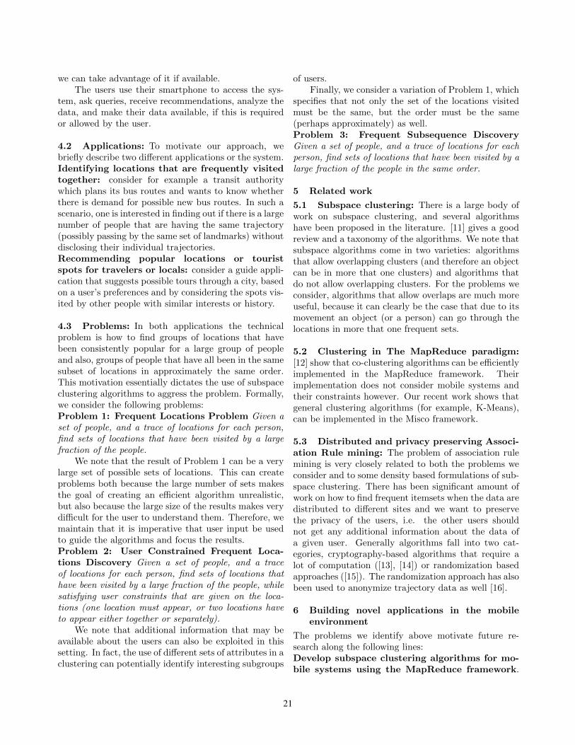
we can take advantage of it if available.The users use their smartphone to access the sys-

tem, ask queries, receive recommendations, analyze thedata, and make their data available, if this is requiredor allowed by the user.

4.2 Applications: To motivate our approach, webriefly describe two different applications or the system.Identifying locations that are frequently visitedtogether: consider for example a transit authoritywhich plans its bus routes and wants to know whetherthere is demand for possible new bus routes. In such ascenario, one is interested in finding out if there is a largenumber of people that are having the same trajectory(possibly passing by the same set of landmarks) withoutdisclosing their individual trajectories.Recommending popular locations or touristspots for travelers or locals: consider a guide appli-cation that suggests possible tours through a city, basedon a user’s preferences and by considering the spots vis-ited by other people with similar interests or history.

4.3 Problems: In both applications the technicalproblem is how to find groups of locations that havebeen consistently popular for a large group of peopleand also, groups of people that have all been in the samesubset of locations in approximately the same order.This motivation essentially dictates the use of subspaceclustering algorithms to aggress the problem. Formally,we consider the following problems:Problem 1: Frequent Locations Problem Given aset of people, and a trace of locations for each person,find sets of locations that have been visited by a largefraction of the people.

We note that the result of Problem 1 can be a verylarge set of possible sets of locations. This can createproblems both because the large number of sets makesthe goal of creating an efficient algorithm unrealistic,but also because the large size of the results makes verydifficult for the user to understand them. Therefore, wemaintain that it is imperative that user input be usedto guide the algorithms and focus the results.Problem 2: User Constrained Frequent Loca-tions Discovery Given a set of people, and a traceof locations for each person, find sets of locations thathave been visited by a large fraction of the people, whilesatisfying user constraints that are given on the loca-tions (one location must appear, or two locations haveto appear either together or separately).

We note that additional information that may beavailable about the users can also be exploited in thissetting. In fact, the use of different sets of attributes in aclustering can potentially identify interesting subgroups

of users.Finally, we consider a variation of Problem 1, which

specifies that not only the set of the locations visitedmust be the same, but the order must be the same(perhaps approximately) as well.Problem 3: Frequent Subsequence DiscoveryGiven a set of people, and a trace of locations for eachperson, find sets of locations that have been visited by alarge fraction of the people in the same order.

5 Related work

5.1 Subspace clustering: There is a large body ofwork on subspace clustering, and several algorithmshave been proposed in the literature. [11] gives a goodreview and a taxonomy of the algorithms. We note thatsubspace algorithms come in two varieties: algorithmsthat allow overlapping clusters (and therefore an objectcan be in more that one clusters) and algorithms thatdo not allow overlapping clusters. For the problems weconsider, algorithms that allow overlaps are much moreuseful, because it can clearly be the case that due to itsmovement an object (or a person) can go through thelocations in more that one frequent sets.

5.2 Clustering in The MapReduce paradigm:[12] show that co-clustering algorithms can be efficientlyimplemented in the MapReduce framework. Theirimplementation does not consider mobile systems andtheir constraints however. Our recent work shows thatgeneral clustering algorithms (for example, K-Means),can be implemented in the Misco framework.

5.3 Distributed and privacy preserving Associ-ation Rule mining: The problem of association rulemining is very closely related to both the problems weconsider and to some density based formulations of sub-space clustering. There has been significant amount ofwork on how to find frequent itemsets when the data aredistributed to different sites and we want to preservethe privacy of the users, i.e. the other users shouldnot get any additional information about the data ofa given user. Generally algorithms fall into two cat-egories, cryptography-based algorithms that require alot of computation ([13], [14]) or randomization basedapproaches ([15]). The randomization approach has alsobeen used to anonymize trajectory data as well [16].

6 Building novel applications in the mobileenvironment

The problems we identify above motivate future re-search along the following lines:Develop subspace clustering algorithms for mo-bile systems using the MapReduce framework.

21

In this context, the Misco system gives an efficienttestbed to develop and test such algorithms. Cur-rent work shows that iterative, non-overlapping clustermethods can be efficiently implemented in a distributedsystem. Several questions have to be addressed how-ever. One of the most important is the developmentof lightweight privacy preserving mechanisms. We notehere that cryptography based approaches may prove dif-ficult to adapt to the mobile environment due to theircomputational requirements.Develop subspace clustering algorthms that in-corporate user constraints. More specifically, wewill investigate different mechanisms to incorporate userconstraints. These constraints can be used to differen-tiate between alternative clusterings, if used after theclustering process, or can be used to guide the cluster-ing approach, if used during the clustering.Distributed techniques for sequential patterndiscovery. We note here that finding frequent con-strained sequential patterns is a problem yet it hasimportant connections to the subspace clustering algo-rithms.

Next we outline future research in addressing thesetopics, and propose extensions to existing work. Cur-rent work focuses on non-overlapping clustering ap-proaches and considers extensions of the iterative clus-tering framework to take into account constraints andidentify interesting subspaces. The non-overlaping clus-tering approach (see for example PROCLUS [17] andrelated work), can be incorporated in our frameworkfollowing the same approach that was taken for com-puting the K-Means algorithm.

The more general, overlapping-cluster approachtypically uses a density based formulation. The fun-damental problem here is that we have to develop amechanism that can use user input to guide the searchamong subspaces since the number of possible subspacesis large. In addition, we have to understand the impactof problems such as sampling (of the dataset and of thesolution space), the effect of horizontal vs vertical parti-tioning of the way data is stored, and of minimizing theinformation shared by the users. Finally, related work[18] has shown that efficient indexing structures can beused with good benefit to identify frequent subspaces,however the problem of developing algorithms for themobile environment is novel.

References

[1] “comscore reports,” http://www.comscore.com/.[2] A. Thiagarajan, L. Ravindranath, K. LaCurts, S. Mad-

den, H. Balakrishnan, S. Toledo, and J. Eriksson,“Vtrack: accurate, energy-aware road traffic delay es-timation using mobile phones,” in SenSys 2009.

[3] B. Bamba, L. Liu, A. Iyengar, and P. S. Yu, “Dis-tributed processing of spatial alarms: A safe region-based approach,” in ICDCS, Washington, DC, 2009,pp. 207–214.

[4] E. Miluzzo, C. Cornelius, A. Ramaswamy, T. Choud-hury, Z. liu, and A. Campbell, “Darwin phones: theevolution of sensing and inference on mobile phones,”in Mobisys 2010, June 15-18, 2010, San Fransisco, CA.

[5] ReadWriteWeb, “Exploring how tobuild a cloud of smartphones,”http://www.readwriteweb.com/cloud/2010/08/nokia-explores-how-to-build-a.php.

[6] E. Miluzzo, N. D. Lane, K. Fodor, R. A. Peterson,H. Lu, M. Musolesi, S. B. Eisenman, X. Zheng, andA. T. Campbell, “Sensing meets mobile social net-works: the design, implementation and evaluation ofthe cenceme application,” in SenSys, 2008.

[7] A. J. Dou, V. Kalogeraki, D. Gunopulos,T. Mielikainen, and V. H. Tuulos, “Schedulingfor real-time mobile mapreduce systems,” in DEBS,2011.

[8] J. Dean and S. Ghemawat, “Mapreduce: Simplifieddata processing on large clusters,” in OSDI, San Fran-cisco, CA, USA, Dec 2004, pp. 137–150.

[9] A. Dou, V. Kalogeraki, D. Gunopulos, T. Mielikinen,V. Tuulos, S. Foley, and C. Yu, “Data clustering on anetwork of mobile smartphones,” in SAINT 2011.

[10] D. Zeinalipour-Yazti, C. Laoudias, M. I. Andreou, andD. Gunopulos, “Disclosure-free gps trace search insmartphone networks,” in Mobile Data Management(1), 2011.

[11] E. Muller, S. Gunnemann, I. Farber, and T. Seidl,“Discovering multiple clustering solutions: Groupingobjects in different views of the data,” in ICDM, 2010.

[12] S. Papadimitriou and J. Sun, “Disco: Distributed co-clustering with map-reduce: A case study towardspetabyte-scale end-to-end mining,” in ICDM, 2008.

[13] M. Kantarcioglu and C. Clifton, “Privacy-preservingdistributed mining of association rules on horizontallypartitioned data,” in DMKD, 2002.

[14] M. G. Kaosar and X. Yi, “Semi-trusted mixer basedprivacy preserving distributed data mining for resourceconstrained devices,” CoRR, vol. abs/1005.0940, 2010.

[15] A. V. Evfimievski, R. Srikant, R. Agrawal, andJ. Gehrke, “Privacy preserving mining of associationrules,” Inf. Syst., vol. 29, no. 4, pp. 343–364, 2004.

[16] M. E. Nergiz, M. Atzori, Y. Saygin, and B. Guc,“Towards trajectory anonymization: a generalization-based approach,” Transactions on Data Privacy, vol. 2,no. 1, pp. 47–75, 2009.

[17] C. C. Aggarwal, C. M. Procopiuc, J. L. Wolf, P. S.Yu, and J. S. Park, “Fast algorithms for projectedclustering,” in SIGMOD Conference, 1999, pp. 61–72.

[18] M. R. Vieira, P. Bakalov, and V. J. Tsotras, “Flextrack:A system for querying flexible patterns in trajectorydatabases,” in SSTD, 2011, pp. 475–480.

22

Multiple Clustering Views via Constrained Projections ∗

Xuan Hong Dang, Ira Assent† James Bailey‡

Abstract

Clustering, the grouping of data based on mutual similarity,

is often used as one of principal tools to analyze and un-

derstand data. Unfortunately, most conventional techniques

aim at finding only a single clustering over the data. For

many practical applications, especially those being described

in high dimensional data, it is common to see that the data

can be grouped into different yet meaningful ways. This

gives rise to the recently emerging research area of discov-

ering alternative clusterings. In this preliminary work, we

propose a novel framework to generate multiple clustering

views. The framework relies on a constrained data projec-

tion approach by which we ensure that a novel alternative

clustering being found is not only qualitatively strong but

also distinctively different from a reference clustering solu-

tion. We demonstrate the potential of the proposed frame-

work using both synthetic and real world datasets and dis-

cuss some future research directions with the approach.

1 Introduction.

Cluster analysis has been widely considered as one ofthe most principal and effective tools in understandingthe data. Given a set of data observations, its objec-tive is to categorize those observations that are similar(under some notion of similarity) into the same clusterwhilst separating dissimilar ones into different clusters.Toward this goal, many algorithms have been developedby which some clustering objective function is proposedalong with an optimization mechanism such as k-means,mixture models, hierarchical agglomerative clustering,graph partitioning, and density-based clustering. A gen-eral observation with these algorithms is that they onlyattempt to produce a single partition over the data. Formany practical applications, especially those being char-acterized in high dimensional data, this objective seemsto be not sufficient since it is common that the dataobservations can be grouped along different yet equallymeaningful ways. For example, when analyzing a docu-

∗Part of this work has been supported by the Danish Council

for Independent Research - Technology and Production Sciences

(FTP), grant 10-081972.†Dept. of Computer Science, Aarhus University, Denmark.

Email: {dang,ira}@cs.au.dk.‡Dept. of Computing and Information Systems, The Univer-

sity of Melbourne, Australia. Email: baileyj@unimelb.edu.au.

ment dataset, one may find that it is possible to catego-rize the documents according to either topics or writingstyles; or when clustering a gene dataset, it is found thatgrouping genes based on their functions or structures isequally important and meaningful [4]. In both theseapplications and many other ones, we may see that thenatural structure behind the observed data is often notunique and there exist many alternative ways to inter-pret the data. Consequently, there is a strong demandto devise novel techniques that are capable of generatingmultiple clustering views regarding the data.

In the literature, several algorithms have been de-veloped to seek alternative clusterings and it is possibleto categorize them into two general approaches: seek-ing alternative clusterings simultaneously [13, 8, 22] andseeking alternative clusterings in sequence [3, 6, 10, 9].In the former approach, all alternative clusterings aresought at the same time whereas in the latter one, eachnovel clustering is found by conditioning on all previousclusterings. From a modeling view point, the latter ap-proach has a major advantage that it limits the numberof cluster parameters needed to be optimized concur-rently.

In this paper, we develop a novel framework tofind multiple clustering views from a provided dataset.Given the data and a reference clustering C(1) as in-puts, our objective is to seek a novel alternative clus-tering that is not only qualitatively strong but also dis-tinctively different from C(1). The proposed algorithmachieves this dual objective by adopting a graph-basedmapping approach that preserves the local neighbor-hood proximity property of the data and further con-forms the constraint of clustering independence with re-spect to C(1). Though our research can be categorizedinto the second approach of sequentially seeking alter-native clusterings, it goes beyond the work in the litera-ture by further ensuring that the geometrical proximityof the data is retained in the lower mapping subspaceand thus naturally reveals clustering structures whichare often masked in the high dimensional data space.We formulate our clustering objective in the frameworkof a constrained eigendecomposition problem and thus ithas a clear advantage that a closed form solution for thelearning subspace always exists and is guaranteed to beglobally optimal. This property contrasts the proposed

23

framework to most existing algorithms, which solely fo-cus on optimizing the single condition of decorrelationand may only achieve a local optimal subspace. Wedemonstrate the potential of the proposed frameworkusing both synthetic and real world data and empiri-cally compare it against several major algorithms in theliterature. Finally, some future studies for our frame-work are discussed and we shortly suggest some poten-tial approaches to deal with them.

2 Related Work.

Though being considered related to subspace cluster-ings [1, 15, 16, 28, 20], the problem of discovering mul-tiple alternative clusterings is relatively young and re-cently it has has been drawing much attention from bothdata mining and machine learning communities. In [19],the authors give an excellent tutorial regarding differentapproaches to the problem. In this section, we adopt thetaxonomy that can generally divide the majority of workin the literature into two approaches: those seeking al-ternative clusterings concurrently and those seeking al-ternative clusterings in sequence, and briefly review thealgorithms that closely related to our research in thispaper.

In the first approach, two algorithms named Dec-kmeans and ConvEM are developed in [13] to find twodisparate clusterings at the same time. In Dec-kmeans,the concept of representative vectors is introduced foreach clustering solution. Subsequently, the objectivefunction of the k-means method is modified by addingterms to account for the orthogonality between meanvectors of one clustering, with respect to the represen-tative vectors of the other. In the ConvEM algorithm,a similar approach is applied by assuming that the datacan be modeled as a sum of mixtures and this work as-sociates each mixture with a clustering solution. Thisleads to the problem of learning a convolution of mix-ture distributions by which the expectation maximiza-tion method can be employed to find the distributions’parameters. Another algorithm called CAMI based onmixture models is developed in [8]. However, instead oftrying to orthogonalize two sets of cluster means, CAMItakes into account a more general concept of mutual in-formation to quantify for the decorrelation between twoclustering models. The algorithm thus attempts to min-imize this quantity while at the same time maximizingthe likelihood of each respective model.

In the second approach, an algorithm namedCOALA is proposed in [3]. Given a known cluster-ing, COALA generates a set of pairwise cannot-link con-straints and it attempts to find a disparate data parti-tion by using these constraints within an agglomerativeclustering process. The NACI algorithm developed in [9]

takes a different approach purely stemming from infor-mation theory. Its clustering objective is thus to max-imize the mutual information between data instancesand cluster labels of the alternative clustering whileminimizing such information between that alternate andthe provided clustering. However, instead of using thetraditional Shannon entropy [5], this work is developedbased on the use of Renyi’s entropy, with the corre-sponding quadratic mutual information [14, 24]. Suchan approach allows the MI to be practically approxi-mated when combined with the non-parametric Parzenwindow technique [23]. Recently, this dual-optimizedclustering objective is also exploited in work [21] withan iterative approach, in contrast to the hierarchicaltechnique adopted in [9]. Another line in the second ap-proach are the algorithms developed in [6, 10, 25] whichaddress the alternative clustering problem via the useof subspace projection. Work in [6] develops two tech-niques to find an alternative clustering using orthogonalprojections. Intuitively, one can characterize a data par-tition by a set of representatives (e.g., cluster means).It is then possible to expect that a dissimilar partitionmight be found by clustering the data in a space orthog-onal to the space spanned by such representatives. Inthe first algorithm in [6], clustering means learnt from agiven partition are used as representatives, whilst in thesecond algorithm, principal components extracted fromsuch centroid vectors are used. A similar approach isdeveloped in [10] in which the transformation is appliedon the distance matrix learnt from the provided cluster-ing. Compared to the two methods developed in [6], thiswork has a benefit that it can further handle the prob-lem of which the data dimension can be smaller thanthe number of clusters (e.g., spatial datasets). Anotherapproach based on data transformation is developed in[25]. This work attempts to transform the data suchthat data instances belonging to the same cluster in thereference clustering are mapped far apart in the newlytransformed space. Our research in this paper is alsoto adopt the data projection approach. However, we gobeyond these related algorithms by ensuring that thenovel projection subspace is not only decorrelated fromthe provided clustering solution, the local similar prop-erty of the data is also preserved in the projection sub-space to strongly support uncovering a novel clusteringstructure behind the data.

3 Problem Definition.

We define our problem of generating multiple clusteringviews from the data as follows.

Given a set X of d-dimensional data in-stances/observations X = {x1,x2, ...,xn} and a clus-tering solution C(1) (i.e., a data partition over X found

24

by any clustering algorithm) over X , we seek an algo-rithm that can learn C(2), a novel clustering solution

from X , whose clusters C(2)i satisfy

⋃i C

(2)i = X and

C(2)i ∩ C

(2)j = ∅ for ∀i 6= j; i, j ≤ K, where K is the

number of expected clusters in C(2)i . The quality of the

alternative clustering should be high and also be dis-tinctively different from C(1). We will here mostly fo-cus on the case where only a single reference clusteringis provided but the framework can be straightforwardlyextended to the general case of generating multiple al-ternative clusterings.

4 The Proposed Framework.

4.1 Subspace Learning Objective with Con-straint. In generating an alternative clustering, ourstudy in this work makes use of a subspace learningapproach. Given C(1) as a reference clustering, we aimto map the data from the original space into a new sub-space in which it is uncorrelated from C(1) whereas themapping also well captures and retains certain prop-erties of the data. The dimension of the subspace isusually smaller than the original one and thus the clus-tering structure behind the data can be more easily un-covered. Clearly, for our clustering problem, we wouldlike that if two instances xi and xj are close in the orig-inal space, they should be mapped also close to eachother in the lower dimensional space. This idea is alsobehind several methods including Local Linear Embed-ding [26], Laplacian Eigenmap [18] and Locality Pre-serving Projection [12]. However, it is worth mentioningthat these algorithms are naturally developed to learn asingle manifold embedded in a high dimensional spaceand to find ways to represent it in an optimal subspace.Our research in this work, despite sharing a similar map-ping objective, is clearly different as we aim to seek a setof clusters from the data and more importantly, furtherrequire the mapping data to be uncorrelated from oneor more reference clusterings.

Following this subspace learning approach, we for-mulate our problem using graph theory. Let G = {V,E}be an undirected graph, where V = {v1, . . . , vn} is a setof vertices and E = {eij} is a set of edges, each con-necting two vertices (vi, vj). A vertex vi corresponds toa data instance xi in the dataset X and the edge eij be-tween vi and vj exists if the respective points xi,xj areclose to each other. Under this setting, the closenessbetween xi and xj can be defined using the ℓ-nearestneighbor concept. Specifically, we define xi to be closeto xj if it is among the ℓ-nearest neighbors of xj or viceversa. Moreover, for the edge connecting two respec-tive vertices vi, vj of such xi and xj , we associate Kij

(computed by the Gaussian function [9]) as a measure of

their closeness degree. For two vertices that are not con-nected, the respective Kij is set to zero. Consequently,we denote K as the n× n matrix having Kij as its ele-ments and it is easy to observe that K is symmetric andtypically sparse, since each vertex is only connected toa limited number of its nearest neighbors.

Given the weight matrix K derived from the graphG and a reference clustering C(1), our objective is tolearn a novel set Y = {y1, . . . ,yn}, where each yi ∈ Rq

is the mapping of xi ∈ Rd, via a projection matrixF , that optimally retains the local neighborhood prox-imity of the original data yet taking the decorrelatedrequirement over the reference solution C(1) into ac-count. Essentially, let us denote X and Y = FTXtwo matrices respectively having xi’s and yi’s as theircolumn vectors and let f be a column in F , then wecan consider f as a transformation vector that linearlycombines X’s dimensions into a 1-dimensional vectoryT = {y1, . . . , yn} = fTX. That means y is one featurein the mapping space Y . We are now able to define oursubspace learning task with the following optimizationfunction:

argminf

1

2

n∑

i=1

n∑

j=1

(fTxi − fTxj)2Kij s.t. STXT f = 0

(4.1)

in which S is a feature subspace that best captures thereference solution C(1) and adding the constant 1/2 doesnot affect our optimization objective. The constraintSTXT f = 0 (or equivalently STy = 0) is crucial sinceit ensures that the mapping dimension is independentfrom S. Also notice that here we assume X is pro-jected onto f to form an R1 optimal subspace, yielding1-dimensional vector yT = {y1, . . . , yn}. The general-ization to q optimal dimensions will be straightforwardonce we derive the solution for f and subsequently y.

Observing from Eq.(4.1) that if Kij is large (im-plying xi and xj are geometrically close in the originalspace), the objective function will be large if the tworespective points yi = fTxi and yj = fTxj are mappedfar apart. Therefore, finding an optimal vector f thatminimizes Eq.(4.1) is equivalent to optimally retainingthe local proximity of the data, subject to the constraintSTXT f = 0 to ensure the decorrelation from C(1).

4.2 Fisher Linear Discriminant for S Selection.We now discuss how to select S, a subspace thatbest captures the provided clustering solution C(1).That means the clusters as components of C(1) canbe well discriminated when data is represented in S.In achieving this goal, the Fisher’s linear discriminant(FDA) can be a natural choice. Briefly, FDA is a

25

supervised learning technique that seeks a direction was a linear combination of the features over X so thatthe within cluster variances are minimized while at thesame time the variances between cluster means and thetotal sample mean are maximized. Mathematically, itsobjective function is represented by:

maxw

wTSBw

wTSWw(4.2)

of which SB and SW respectively being called thebetween-cluster scatter matrix and within-cluster scat-ter matrix. They are calculated by:

SB =∑

k

nk(m(k) −m)(m(k) −m)T and

SW =∑

k

nk∑

i

(x(k)i −m(k))(x

(k)i −m(k))T

with m(k) and m are respectively the cluster mean ofthe k-th cluster and the total sample mean, and nk isthe number of instances grouped in k-th cluster. Solvingthis problem results in that w is the eigenvector corre-sponding to the largest eigenvalue of the matrix S−1

W SB .Usually in practice, when the number of clusters is only2, one may need only a single dimension w to capturethe solution. For a more general case where the numberof clusters is q+1, a set of q eigenvectorsw’s correspond-ing to the q largest eigenvalues of S−1

W SB are selected.Therefore in our approach, we choose such q eigenvec-tors as the optimal subspace S encoding for C(1). Eachrow in S corresponds to a projected data instance andthe number of columns in S equals to the number ofretained eigenvectors. Recall that the projected datainstances in S strongly support the reference cluster-ing C(1) (i.e., highly correlated to the cluster labels inC(1)). Consequently, by taking the orthogonal condi-tion of STy, the newly mapped data, the yi’s, shouldbe decorrelated from the reference solution C(1).

4.3 Solving the Constrained Objective Func-tion. For solving the objective function with the con-straint in Eq.(4.1), we can use the Lagrange method.First, let D be the diagonal matrix with Dii =

∑j Kij

and let L = D − K, then by expanding the sum inEq.(4.1), we can obtain the following function:

∑

i,j

fTxiKijxTi f −

∑

i,j

fTxiKijxTj f (4.3)

=∑

i

fTxiDiixTi f − fTXKXT f

= fTXDXT f − fTXKXf

= fTXLXT f

We need to put another constraint fTXDXT f = 1to remove f ’s scaling factor. Then using the Lagrangemethod with two Lagrange multipliers α and β, we solvethe following function:

L(α, β, f) = fTXLXT f − α(fTXDXT f − 1)− βSTXT f(4.4)

For simplicity, let us denote:

L = XLXT

D = XDXT and

S = XS

It is easy to verify that D is symmetric and positivesemi-definite. Moreover, there exists D−1/2 and itstranspose being identical. We therefore change thevariable f = D−1/2z. It follows that:

fT Lf = zT D−1/2LD−1/2z = zTQz

and the two constraints respectively are:

fT Df = zT z = 1

ST f = ST D−1/2z = 0

Hence, our Lagrange function can be re-written asfollows:

L(α, β, z) = 1

2zTQz− 1

2α(zT z− 1)− βUT z (4.5)

of which we have used UT to denote ST D−1/2 andadding the constant 1/2 does not affect our optimizationobjective. Taking the derivative of L(α, β, z) withrespect to z and setting it equal to zero give us:

δLδz

= Qz− αz− βU = 0 (4.6)

Left multiplying UT to both sides results in β =(UTU)−1UTQz and substituting it into Eq.(4.6), wederive:

26

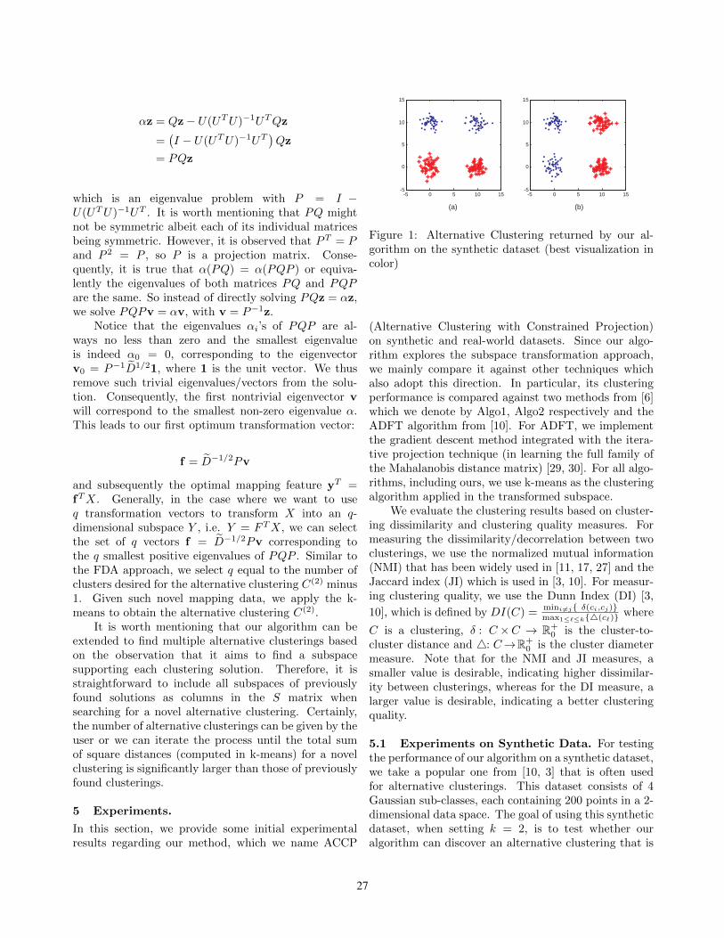
αz = Qz− U(UTU)−1UTQz

=(I − U(UTU)−1UT

)Qz

= PQz

which is an eigenvalue problem with P = I −U(UTU)−1UT . It is worth mentioning that PQ mightnot be symmetric albeit each of its individual matricesbeing symmetric. However, it is observed that PT = Pand P 2 = P , so P is a projection matrix. Conse-quently, it is true that α(PQ) = α(PQP ) or equiva-lently the eigenvalues of both matrices PQ and PQPare the same. So instead of directly solving PQz = αz,we solve PQPv = αv, with v = P−1z.

Notice that the eigenvalues αi’s of PQP are al-ways no less than zero and the smallest eigenvalueis indeed α0 = 0, corresponding to the eigenvectorv0 = P−1D1/21, where 1 is the unit vector. We thusremove such trivial eigenvalues/vectors from the solu-tion. Consequently, the first nontrivial eigenvector vwill correspond to the smallest non-zero eigenvalue α.This leads to our first optimum transformation vector:

f = D−1/2Pv

and subsequently the optimal mapping feature yT =fTX. Generally, in the case where we want to useq transformation vectors to transform X into an q-dimensional subspace Y , i.e. Y = FTX, we can selectthe set of q vectors f = D−1/2Pv corresponding tothe q smallest positive eigenvalues of PQP . Similar tothe FDA approach, we select q equal to the number ofclusters desired for the alternative clustering C(2) minus1. Given such novel mapping data, we apply the k-means to obtain the alternative clustering C(2).

It is worth mentioning that our algorithm can beextended to find multiple alternative clusterings basedon the observation that it aims to find a subspacesupporting each clustering solution. Therefore, it isstraightforward to include all subspaces of previouslyfound solutions as columns in the S matrix whensearching for a novel alternative clustering. Certainly,the number of alternative clusterings can be given by theuser or we can iterate the process until the total sumof square distances (computed in k-means) for a novelclustering is significantly larger than those of previouslyfound clusterings.

5 Experiments.

In this section, we provide some initial experimentalresults regarding our method, which we name ACCP

-5 0 5 10 15 -5

0

5

10

15

-5 0 5 10 15 -5

0

5

10

15

(b) (a)

Figure 1: Alternative Clustering returned by our al-gorithm on the synthetic dataset (best visualization incolor)

(Alternative Clustering with Constrained Projection)on synthetic and real-world datasets. Since our algo-rithm explores the subspace transformation approach,we mainly compare it against other techniques whichalso adopt this direction. In particular, its clusteringperformance is compared against two methods from [6]which we denote by Algo1, Algo2 respectively and theADFT algorithm from [10]. For ADFT, we implementthe gradient descent method integrated with the itera-tive projection technique (in learning the full family ofthe Mahalanobis distance matrix) [29, 30]. For all algo-rithms, including ours, we use k-means as the clusteringalgorithm applied in the transformed subspace.

We evaluate the clustering results based on cluster-ing dissimilarity and clustering quality measures. Formeasuring the dissimilarity/decorrelation between twoclusterings, we use the normalized mutual information(NMI) that has been widely used in [11, 17, 27] and theJaccard index (JI) which is used in [3, 10]. For measur-ing clustering quality, we use the Dunn Index (DI) [3,

10], which is defined by DI(C) =mini6=j{ δ(ci,cj)}max1≤ℓ≤k{△(cℓ)} where

C is a clustering, δ : C ×C → R+0 is the cluster-to-

cluster distance and △: C→R+0 is the cluster diameter

measure. Note that for the NMI and JI measures, asmaller value is desirable, indicating higher dissimilar-ity between clusterings, whereas for the DI measure, alarger value is desirable, indicating a better clusteringquality.

5.1 Experiments on Synthetic Data. For testingthe performance of our algorithm on a synthetic dataset,we take a popular one from [10, 3] that is often usedfor alternative clusterings. This dataset consists of 4Gaussian sub-classes, each containing 200 points in a 2-dimensional data space. The goal of using this syntheticdataset, when setting k = 2, is to test whether ouralgorithm can discover an alternative clustering that is

27

0

0.4

0.8

1.2

1.6

2

Algo1 Algo2 ADFT ACCP

Dun

n In

dex

0

0.1

0.2

0.3

0.4

0.5

0.6

Algo1 Algo2 ADFT ACCP

Nor

mal

ized

Mut

ual I

nfor

mat

ion

0

0.1

0.2

0.3

0.4

0.5

0.6

Algo1 Algo2 ADFT ACCP

Jacc

ard

Inde

x

Figure 2: Clustering performance returned by fouralgorithms on the Cloud data

orthogonal to the existing one. In Figure 1, we show theclustering results returned by our algorithm. Given thereference clustering C(1) which groups two Gaussians onthe top and two Gaussians in the bottom as each cluster(shown in Figure 1(a)), ACCP successfully uncoversthe alternative clustering C(2) which categorizes twoGaussians on the left and two ones on the right asclusters (shown in Figure 1(b)).

5.2 Experiments on the UCI data. We use tworeal-world datasets from the UCI KDD repository [2]to compare the performance of our algorithm againstthe other techniques. The first dataset is the Clouddata which consists of data collected from a cloud-seeding experiment in Tasmania in the time betweenmid-1964 and January 1971. For a reference clustering,we run the k-means algorithm (with K = 4 as thenumber of clusters) and its resultant clustering is used

0

0.2

0.4

0.6

0.8

1

1.2

Algo1 Algo2 ADFT ACCP

Dun

n In

dex

0

0.05

0.1

0.15

0.2

0.25

0.3

Algo1 Algo2 ADFT ACCP

Nor

mal

ized

Mut

ual I

nfor

mat

ion

0

0.1

0.2

0.3

0.4

Algo1 Algo2 ADFT ACCP

Jacc

ard

Inde

x

Figure 3: Clustering performance returned by fouralgorithms on the Housing data

as the reference solution for all algorithms. The seconddataset is the Housing data which consists informationabout the housing values collected in Boston’s suburbs.Similar to the Cloud data, we apply k-means algorithmon this dataset and use it as the reference solution forall algorithms. We show the clustering performance ofall techniques in Figures 2 and 3 respectively for theCloud and Housing data.

As observed from all figures, our algorithm performsbetter than two techniques developed in [6] and theADFT one in [10]. Its clustering dissimilarity measuringby the normalized mutual information and the JaccardIndex is lower than that of Algo1, Algo2 and ADFTwhereas the clustering quality quantified by the DunnIndex is higher. This advantage can be justified bythe approach of ACCP. Though all algorithms adopta linear projection technique to derive a novel subspacethat is decorrelated from the reference clustering, the

28

ACCP further takes into account the local neighborhoodproximity of the data by retaining that property in thenovel low dimensional subspace. The novel clusteringstructure in this learnt subspace therefore is moreprominent compared to that of the other techniqueswhich only attempt to minimize the correlation betweentwo subspaces. Moreover, though the derived subspaceof all techniques is ensured to be independent fromthe provided clustering, it is still possible that thealternative learnt from that subspace might not stronglydecorrelated since there is a need to optimize for theclustering objective function as well. This generallyexplains for the difference in the NMI and JI measuresof all methods.

6 Conclusions and Future Studies.

In this paper, we have addressed an important problemof uncovering multiple clustering views from a givendataset. We propose the ACCP framework to learna novel lower dimensional subspace that is not onlydecorrelated from the provided reference clustering butthe local geometrical proximity of the data is alsobeing retained. By the second objective, our workgoes beyond the others, which also adopt a subspacelearning approach for seeking alternative clusterings, yetonly focus on the dissimilarity property of the novelclustering. More importantly, we have demonstratedour dual-objective can be formulated via a constrainedsubspace learning problem of which a global optimumsolution can be achieved.

Several initial empirical results of the proposedframework over the synthetic and real world datasetsare given. Certainly, these results remain preliminaryand more experimental work should be done in orderto provide more insights into its performance. Addi-tionally, though our framework is claimed to be capableof finding multiple clustering views, its performance onsome suitable datasets has not been verified. Determin-ing an ideal number of alternative clusterings still needsto be formally addressed. We leave these problems asan important and immediate task of the future work.

In addition to the above issues, our research in thispaper opens up some potential and interesting direc-tions for future studies. Specifically, despite advancingthe subspace based learning approach for the alternativeclustering problem, our research has exploited a hardconstraint solution to ensure alternatives’ dissimilarity.Such an approach might be too strict in some practicalapplications and thus some novel approaches based onsoft constraints could be interesting. This implies that atrade-off factor between two criteria of subspaces’ inde-pendence and intrinsic data structure retaining can beintroduced, or we can constrain the subspace’s decor-

relation criteria to no less than a given threshold. Ineither of the two cases, a data-adaptive learning tech-nique is required and the compromise between two fac-tors is worth to study both theoretically and empirically.Furthermore, our research has not yet focused on the in-terpretation regarding the resultant alternative cluster-ings. This is an important problem, especially from theuser perspective. Which features are best to describe aclustering solution and which ones are least correlatedwith respect to that solution are all informative to theuser in understanding the data. Compared to a nonlin-ear subspace learning approach [7], our research direc-tion in this work is beneficial due to its linear subspacelearning approach. That means the linear combinationamongst the original features is explicitly represented inthe transformation matrix F . However, seeking for anoptimal and concise set of features that best character-izes for a clustering solution is still a challenging issuegiven the fact that the number of original data featuresis usually huge. We believe that these open issues areworth to be further explored and studied.

References

[1] I. Assent, E. Muller, S. Gunnemann, R. Krieger, andT. Seidl. Less is more: Non-redundant subspaceclustering. In 1st MultiClust International Workshopin conjunction with 16th ACM SIGKDD., 2010.

[2] A. Asuncion and D.J. Newman. UCI machine learningrepository, 2007.

[3] E. Bae and J. Bailey. COALA: A novel approach forthe extraction of an alternate clustering of high qualityand high dissimilarity. In The IEEE InternationalConference on Data Mining., pages 53–62, 2006.

[4] G. Chechik and N. Tishby. Extracting relevant struc-tures with side information. In International Con-ference on Neural Information Processing Systems(NIPS), 2002.

[5] T. M. Cover and J. A. Thomas. Elements of Informa-tion Theory. Wiley-Interscience, August 1991.

[6] Y. Cui, X. Fern, and J. Dy. Non-redundant multi-view clustering via orthogonalization. In The IEEEInternational Conference on Data Mining, pages 133–142, 2007.

[7] X.H. Dang and J. Bailey. Generating multiple alterna-tive clusterings via globally optimal subspaces. UnderReview.

[8] X.H. Dang and J. Bailey. Generation of alternativeclusterings using the cami approach. In SIAM Interna-tional Conference on Data Mining (SDM), pages 118–129, 2010.

[9] X.H. Dang and J. Bailey. A hierarchical informationtheoretic technique for the discovery of non linear alter-native clusterings. In ACM Conference on KnowledgeDiscovery and Data Mining (SIGKDD), pages 573–582, 2010.

29

[10] I. Davidson and Z. Qi. Finding alternative clusteringsusing constraints. In The IEEE International Confer-ence on Data Mining, pages 773–778, 2008.

[11] X. Fern and W. Lin. Cluster ensemble selection. Stat.Anal. Data Ming, 1(3):128–141, 2008.

[12] X. He and P. Niyogi. Locality preserving projections.In International Conference on Neural InformationProcessing Systems (NIPS), 2003.

[13] P. Jain, R. Meka, and I. Dhillon. Simultaneous unsu-pervised learning of disparate clusterings. In SIAM In-ternational Conference on Data Mining (SDM), pages858–869, 2008.

[14] J. Kapur. Measures of Information and their Applica-tion. John Wiley, 1994.

[15] H.-P. Kriegel, E. Schubert, and A. Zimek. Evalu-ation of multiple clustering solutions. In 2nd Mul-tiClust International Workshop in conjunction withECML/PKDD, 2011.

[16] H.-P. Kriegel and A. Zimek. Subspace clustering,ensemble clustering, alternative clustering, multiviewclustering: What can we learn from each other. In 1stMultiClust International Workshop in conjunction with16th ACM SIGKDD, 2010.

[17] M. Law, A. Topchy, and A. Jain. Multiobjective dataclustering. In CVPR Conference, pages 424–430, 2004.

[18] B. Mikhail and N. Partha. Laplacian eigenmapsand spectral techniques for embedding and clustering.In International Conference on Neural InformationProcessing Systems (NIPS), pages 585–591, 2001.

[19] E. Muller, S. Gunnemann, I. Farber, and T. Seidl. Dis-covering multiple clustering solutions: Grouping ob-jects in different views of the data (tutorial). In SIAMInternational Conference on Data Mining (SDM),2011.

[20] Emmanuel Muller, Ira Assent, Stephan Gunnemann,Patrick Gerwert, Matthias Hannen, Timm Jansen,and Thomas Seidl. A framework for evaluation andexploration of clustering algorithms in subspaces ofhigh dimensional databases. In BTW, pages 347–366,2011.

[21] X. V. Nguyen and J. Epps. minCEntropy: a novelinformation theoretic approach for the generation ofalternative clusterings. In The IEEE InternationalConference on Data Mining, pages 521–530, 2010.

[22] D. Niu, J. G. Dy, and M. I. Jordan. Multiple non-redundant spectral clustering views. In ICML, pages831–838, 2010.

[23] E. Parzen. On estimation of a probability densityfunction and mode. The Annals of MathematicalStatistics, 33(3):1065–1076, 1962.

[24] J. Principe, D. Xu, and J. Fisher. Information Theo-retic Learning. John Wiley & Sons, 2000.

[25] Z. Qi and I. Davidson. A principled and flexibleframework for finding alternative clusterings. In ACMConference on Knowledge Discovery and Data Mining(SIGKDD), pages 717–726, 2009.

[26] T. R. Sam and K. S. Lawrence. Nonlinear dimension-ality reduction by locally linear embedding. Science

Journal, 290(5500):2323–2326, 2000.[27] A. Topchy, A. Jain, and W. Punch. A mixture model

for clustering ensembles. In SDM Conference, 2004.[28] J. Vreeken and A. Zimek. When pattern met subspace

cluster - a relationship story. In 2nd MultiClust Inter-national Workshop in conjunction with ECML/PKDD,2011.

[29] E. Xing, A. Ng, M. Jordan, and S. Russell. Distancemetric learning with application to clustering with side-information. In International Conference on NeuralInformation Processing Systems (NIPS), pages 505–512, 2002.

[30] L. Yang and R. Jin. Distance metric learning: Acomprehensive survey, 2006.

30

Explorative Multi-View Clustering Using Frequent-Groupings

Martin Hahmann, Markus Dumat, Dirk Habich, Wolfgang LehnerDresden University of Technology

Database Technology GroupDresden Germany

firstname.lastname@tu-dresden.de

Abstract

In this paper, we present our novel clustering technique

called frequent-groupings as combination of alternative and

ensemble clustering. Our new approach combines the benefit

of both underlying concepts in an integrated way and allows

the creation of robust clustering alternatives. In detail, we

present (1) different approaches for the automatic creation

of alternatives, (2) a user-guided exploratory extraction

process and (3) an evaluation method to compare extracted

alternatives with regards to their similarities.

1 Introduction

The relevance of clustering as a data analysis techniqueis more and more increasing. This is due to the ongoingtrend for data gathering, that spreads in different areasof research and industry. In general, data clustering isdescribed as the problem of (semi)-automatic partition-ing of a set of objects into groups, called clusters, so thatobjects in the same cluster are similar, while objects indifferent clusters are dissimilar. The identification ofsimilarities between data objects and their arrangementinto groups with regard to these similarities, are essen-tial tools to gain understanding and acquire previouslyunknown knowledge.

As this technique is quite powerful, its applicationby humans offers several challenges that need to be tack-led, because they have a significant influence on theclustering result. One challenge e.g. is the selectionof the best-fitting clustering algorithm for the dataset.A multitude of clustering algorithms has been developedover the years. These traditional algorithms have sev-eral limitations. On the one hand, they are not generallyapplicable, meaning that certain algorithms and param-eterizations only suit certain datasets. On the otherhand, traditional techniques generate only a single clus-tering result, but as todays data sets become more com-plex and high-dimensional there often are multiple validclustering results possible for a single dataset. Besidesthese data centric problems, usability and applicabil-ity have become important issues as clustering evolves

from a niche application in research to a widespreadanalysis technique employed in an increasing number ofareas. With this trend, more users come into contactwith clustering, who are often experts of their respec-tive application domain but have no experience in thearea of clustering. This calls for clustering approachesthat can be versatilely applied and lack the complicatedalgorithm selection and configuration of traditional ap-proaches.

In recent years, a number of approaches have beenintroduced to tackle some of these issues. The area ofalternative clustering [2, 3] provides multiple cluster-ing solutions for a dataset. With this, several views oncomplex data can be offered, and the very availabilityof multiple clusterings usually can free the user fromadjusting a single clustering that proves unsatisfactory.An opposing approach is ensemble clustering [4, 9] inwhich a set of multiple clusterings is integrated to forma single consensus solution. This input set is also calledclustering-ensemble and contains results that are gen-erated using different algorithms and parameters. Theconsensus result is often more robust than clusteringsgenerated by a single algorithm and set of parameters,which means that this technique is more versatile interms of application. Additionally, algorithm selectionand configuration is eased as a range of methods and pa-rameters is utilized instead of a single configuration. Onthe downside, ensemble clustering provides just one so-lution and therefore resembles traditional clustering atthat point. To create an alternative consensus cluster-ing, the user has to re-configure the clustering-ensembleby changing algorithms and/or parameters. This is avery challenging task because multiple algorithms mustbe selected and configured.

The concepts of alternative clustering and ensem-ble clustering have their own benefits compared to tra-ditional clustering approaches. However, to tackle allchallenging issues of clustering from a users perspec-tive, a combination of both concepts would be benefi-cial. In [6], we already introduced our hybrid concept

31

called frequent-groupings. This novel technique is basedon the idea of frequent-itemset mining [1] and allows (1)the identification of robust clusters, occurring through-out the clustering-ensemble and (2) the derivation ofrobust alternative clustering results. After summariz-ing our concept of [6] in Section 2, we contribute thefollowing detailed aspects to our hybrid concept in thispaper:

1. We describe different automated approaches for theextraction of alternative clusterings in Section 3.

2. We propose a method for the explorative extractionof robust clustering alternatives and describe a wayto measure their similarities in Section 4

Finally, we conclude the paper with some remarksregarding future work in Section 5 and a brief summaryin Section 6.

2 Frequent Groupings

In our previous work [6], we described the conceptof frequent-groupings as a means to combine benefitsfrom the area of alternative clusterings and ensembleclustering. Using frequent-groupings, it is possibleto combine clusters with an increased robustness intoalternative clustering solutions.

The core idea of our approach originates from thearea of ensemble-clustering [5], in which a single con-sensus solution is generated from an ensemble of dif-ferent clusterings. Such a consensus solution is gener-ated by identifying sets of objects, that are frequentlyassigned to the same cluster throughout the clustering-ensemble. These sets, then become the clusters of theconsensus result and form a clustering, whose objectassignments agree with the majority of the members ofthe clustering-ensemble.

Lets assume a dataset D = {x1, x2, . . . , xn} ofobjects in a multidimensional feature space, and aclustering-ensemble C = {C1, C2, . . . , Ck} that containsk clusterings of D, each with a different number of clus-ters and different cluster composition. In general, thereare two ways to evaluate the similarities of the clus-ter assignments of an object throughout the ensemble:(i) label-based approaches that match clusters [9] and(ii) approaches based on counting pairwise-similaritiesand the co-occurence of object pairs [4]. Our frequent-groupings approach [6] offers an alternative to thesetwo principles and is based on the concept of frequent-itemsets [1].

Assuming a set of n items I = {i1, i2, . . . , in} anda set of transactions T = {t1, . . . , tm} of which eachtransaction has a unique id an contains a subset of I, aset of items X is called frequent if its support exceeds a

given threshold. The support of an itemset X is definedby the fraction of transactions of T that contain X . Atthis point, the analogy to ensemble clustering should beobvious: while frequent-itemsets aim to identify itemsthat co-occur in many transitions, ensemble clusteringsearches for objects occuring together in the majorityof clusters. For our frequent-groupings approach, wemap the concepts of I, T and support to the domainof ensemble-clustering, whereas I corresponds to thedataset and T corresponds to the clusters of the ensem-ble. According to these mappings, the support of a setof data objects X shows the fraction of the clustering-ensemble, in which X is part of the same cluster. Ifsupport(X ) exceeds a certain threshold, we call X afrequent-grouping.

To illustrate our frequent-groupings idea, we regarda small example from our previous work [6], featuring adataset D = {x1, x2, . . . , x9} and a clustering-ensembleC containing the following 4 clusterings:

• C1 = {(x1, x2, x3) (x4, x5, x6) (x7, x8, x9)}• C2 = {(x1, x2, x3) (x4, x5, x7, x9) (x6, x8)}• C3 = {(x2) (x1, x3, x4, x5)(x6) (x7, x8, x9)}• C4 = {(x1, x2, x3) (x4, x5) (x6, x8) (x7, x9)}

For frequent-grouping generation, we specify a minimalsupport threshold of 50%, meaning that objects occur-ing together in at least 2 clusterings of the ensembleare considered as frequent in our example. Figure 1shows the frequent-groupings generated from the de-scribed setting.

The generation of frequent-groupings does not re-sult in a simple list of object sets but in a more complexgraph-like structure. This structure consists of nodesrepresenting the frequent-groupings and edges showingsubset/superset relations between frequent-groupings.Each node contains three values: (i) an id , (ii) a num-ber showing the support of the grouping, and (iii) theobjects that are part of this grouping. Besides the ninenodes with an id, there are several greyed-out nodes inthe figure. These represent groupings that occur in theclustering-ensemble but do not meet the required mini-mal support and are thus filtered out. For example, eachof three nodes in the upper part of Figure 1 occurs onlyin one of the clusterings of the ensemble. In order tofurther limit the number of actual frequent-groupings,we require that all frequent-groupings are closed, whichmeans that no frequent-grouping fgX is a subset of an-other frequent-grouping fgY that has the same supportas fgX. In compliance with this closed constraint the re-maining greyed-out nodes at the base of the graph arerejected as valid frequent-groupings. As already men-tioned, the edges of the graph show relations between

32

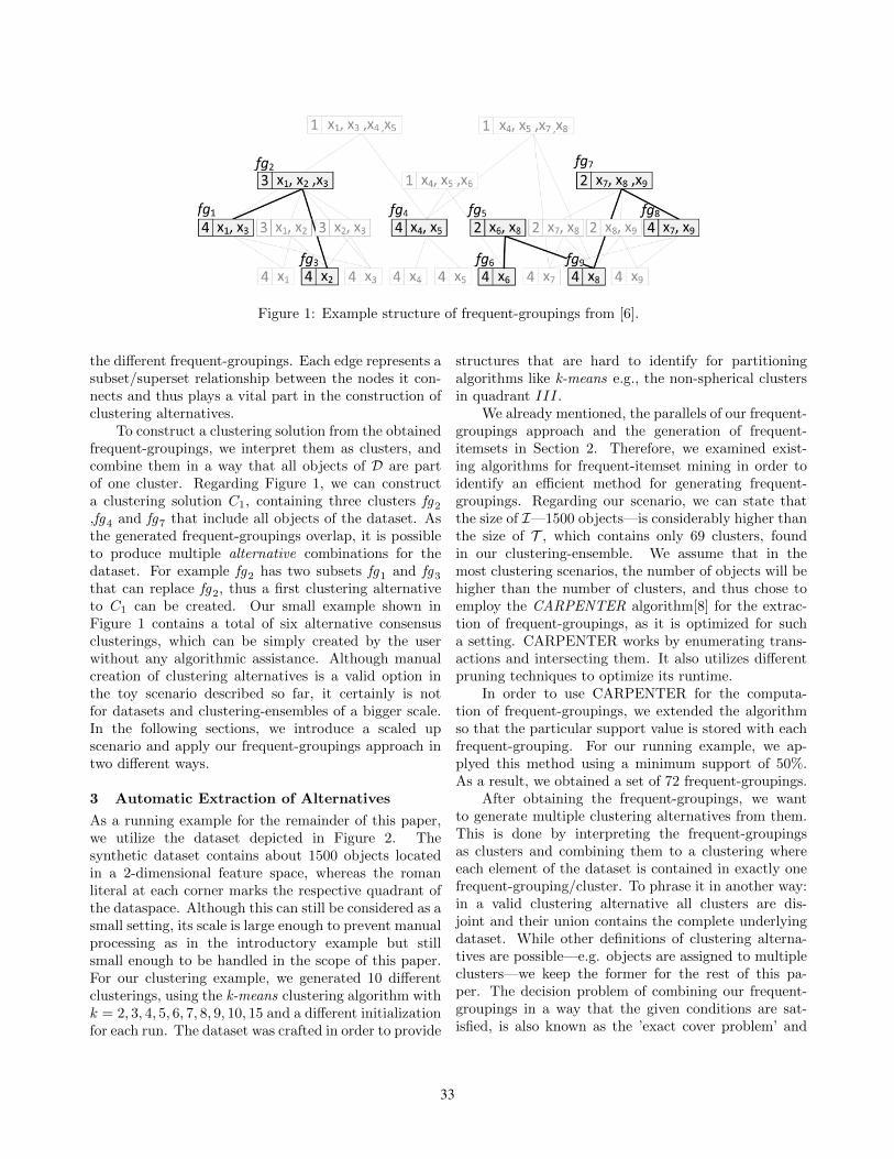
Figure 1: Example structure of frequent-groupings from [6].

the different frequent-groupings. Each edge represents asubset/superset relationship between the nodes it con-nects and thus plays a vital part in the construction ofclustering alternatives.

To construct a clustering solution from the obtainedfrequent-groupings, we interpret them as clusters, andcombine them in a way that all objects of D are partof one cluster. Regarding Figure 1, we can constructa clustering solution C1, containing three clusters fg2

,fg4 and fg7 that include all objects of the dataset. Asthe generated frequent-groupings overlap, it is possibleto produce multiple alternative combinations for thedataset. For example fg2 has two subsets fg1 and fg3

that can replace fg2, thus a first clustering alternativeto C1 can be created. Our small example shown inFigure 1 contains a total of six alternative consensusclusterings, which can be simply created by the userwithout any algorithmic assistance. Although manualcreation of clustering alternatives is a valid option inthe toy scenario described so far, it certainly is notfor datasets and clustering-ensembles of a bigger scale.In the following sections, we introduce a scaled upscenario and apply our frequent-groupings approach intwo different ways.

3 Automatic Extraction of Alternatives

As a running example for the remainder of this paper,we utilize the dataset depicted in Figure 2. Thesynthetic dataset contains about 1500 objects locatedin a 2-dimensional feature space, whereas the romanliteral at each corner marks the respective quadrant ofthe dataspace. Although this can still be considered as asmall setting, its scale is large enough to prevent manualprocessing as in the introductory example but stillsmall enough to be handled in the scope of this paper.For our clustering example, we generated 10 differentclusterings, using the k-means clustering algorithm withk = 2, 3, 4, 5, 6, 7, 8, 9, 10, 15 and a different initializationfor each run. The dataset was crafted in order to provide

structures that are hard to identify for partitioningalgorithms like k-means e.g., the non-spherical clustersin quadrant III.

We already mentioned, the parallels of our frequent-groupings approach and the generation of frequent-itemsets in Section 2. Therefore, we examined exist-ing algorithms for frequent-itemset mining in order toidentify an efficient method for generating frequent-groupings. Regarding our scenario, we can state thatthe size of I—1500 objects—is considerably higher thanthe size of T , which contains only 69 clusters, foundin our clustering-ensemble. We assume that in themost clustering scenarios, the number of objects will behigher than the number of clusters, and thus chose toemploy the CARPENTER algorithm[8] for the extrac-tion of frequent-groupings, as it is optimized for sucha setting. CARPENTER works by enumerating trans-actions and intersecting them. It also utilizes differentpruning techniques to optimize its runtime.

In order to use CARPENTER for the computa-tion of frequent-groupings, we extended the algorithmso that the particular support value is stored with eachfrequent-grouping. For our running example, we ap-plyed this method using a minimum support of 50%.As a result, we obtained a set of 72 frequent-groupings.

After obtaining the frequent-groupings, we wantto generate multiple clustering alternatives from them.This is done by interpreting the frequent-groupingsas clusters and combining them to a clustering whereeach element of the dataset is contained in exactly onefrequent-grouping/cluster. To phrase it in another way:in a valid clustering alternative all clusters are dis-joint and their union contains the complete underlyingdataset. While other definitions of clustering alterna-tives are possible—e.g. objects are assigned to multipleclusters—we keep the former for the rest of this pa-per. The decision problem of combining our frequent-groupings in a way that the given conditions are sat-isfied, is also known as the ’exact cover problem’ and

33

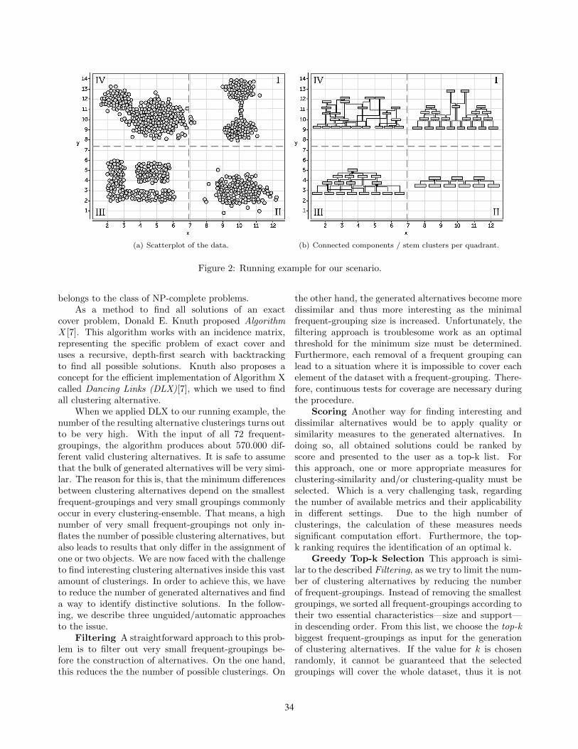
(a) Scatterplot of the data. (b) Connected components / stem clusters per quadrant.

Figure 2: Running example for our scenario.

belongs to the class of NP-complete problems.As a method to find all solutions of an exact

cover problem, Donald E. Knuth proposed AlgorithmX [7]. This algorithm works with an incidence matrix,representing the specific problem of exact cover anduses a recursive, depth-first search with backtrackingto find all possible solutions. Knuth also proposes aconcept for the efficient implementation of Algorithm Xcalled Dancing Links (DLX)[7], which we used to findall clustering alternative.

When we applied DLX to our running example, thenumber of the resulting alternative clusterings turns outto be very high. With the input of all 72 frequent-groupings, the algorithm produces about 570.000 dif-ferent valid clustering alternatives. It is safe to assumethat the bulk of generated alternatives will be very simi-lar. The reason for this is, that the minimum differencesbetween clustering alternatives depend on the smallestfrequent-groupings and very small groupings commonlyoccur in every clustering-ensemble. That means, a highnumber of very small frequent-groupings not only in-flates the number of possible clustering alternatives, butalso leads to results that only differ in the assignment ofone or two objects. We are now faced with the challengeto find interesting clustering alternatives inside this vastamount of clusterings. In order to achieve this, we haveto reduce the number of generated alternatives and finda way to identify distinctive solutions. In the follow-ing, we describe three unguided/automatic approachesto the issue.

Filtering A straightforward approach to this prob-lem is to filter out very small frequent-groupings be-fore the construction of alternatives. On the one hand,this reduces the the number of possible clusterings. On

the other hand, the generated alternatives become moredissimilar and thus more interesting as the minimalfrequent-grouping size is increased. Unfortunately, thefiltering approach is troublesome work as an optimalthreshold for the minimum size must be determined.Furthermore, each removal of a frequent grouping canlead to a situation where it is impossible to cover eachelement of the dataset with a frequent-grouping. There-fore, continuous tests for coverage are necessary duringthe procedure.

Scoring Another way for finding interesting anddissimilar alternatives would be to apply quality orsimilarity measures to the generated alternatives. Indoing so, all obtained solutions could be ranked byscore and presented to the user as a top-k list. Forthis approach, one or more appropriate measures forclustering-similarity and/or clustering-quality must beselected. Which is a very challenging task, regardingthe number of available metrics and their applicabilityin different settings. Due to the high number ofclusterings, the calculation of these measures needssignificant computation effort. Furthermore, the top-k ranking requires the identification of an optimal k.

Greedy Top-k Selection This approach is simi-lar to the described Filtering, as we try to limit the num-ber of clustering alternatives by reducing the numberof frequent-groupings. Instead of removing the smallestgroupings, we sorted all frequent-groupings according totheir two essential characteristics—size and support—in descending order. From this list, we choose the top-kbiggest frequent-groupings as input for the generationof clustering alternatives. If the value for k is chosenrandomly, it cannot be guaranteed that the selectedgroupings will cover the whole dataset, thus it is not

34

possible to guarantee that even one clustering can beconstructed. In order to make sure that at least onevalid result is generated, we used a kind of brute-forceapproach, i.e. we start with k = 1 and execute ourDLX implementation. If no result is returned k is incre-mented and the algorithm is run again. This is repeateduntil at least one clustering is returned. Although thisapproach is not very elegant, it can narrow the gener-ated alternatives down to a number in the single dig-its. However, after continued testing we found out thatthe effectiveness of this method is unpredictable and de-pends highly on the underlying clustering-ensemble. Weapplied the described procedure, using the dataset fromour running example and different ensemble configura-tions. Some configurations returned 10 or less alterna-tives, while other configurations returned much largerresult sets, containing up to 300.000 clustering alterna-tives.

None of the approaches is optimal to reach ourgoal of finding a compact set of interesting clusteringalternatives. Therefore we introduce an additionalapproach in the following section, that reaches thedescribed goal by including the user into the processof building robust clustering alternatives.

4 Explorative Extraction of Alternatives

In the previous section, we showed that the straight-forward automatic extraction of clustering alternativesleaves the user with a very large set of results, of whichmost will be very similar. To tackle this issue, we de-scribed some approaches that aim to create not all, buta compact set of distinctive clustering alternatives. Allof these automatic approaches for extraction have draw-backs, mostly due to configuration challenges and pre-dictability. As full automation of the extraction seemsto be suboptimal, we incorporate the user into the gen-eration process, thus allowing an explorative creation ofclustering alternatives.

The core idea of this kind of extraction is to use thegraph structure of our frequent-groupings as guidancefor the creation of clustering alternatives. Lets look atthe graph of frequent-groupings of our running exam-ple. After generating all 72 frequent-groupings with aminimal support of 50%, this graph consists of the 4connected components shown in Figure 2(b), of whicheach represents one quadrant of our dataspace. Thisone-to-one correspondence is random and results fromour clustering-ensemble. Different ensemble configura-tions will also lead to different connected components.These connected components form the starting point ofour explorative extraction and we will refer to them asstem clusters. All stem clusters are disjoint and theirunion contains all objects of the dataset. Therefore we

could derive a clustering solution with 4 clusters fromthis setting. However, such a clustering would not bea valid result. It would not correctly represent the oc-currence of clusters in the clustering ensemble, but justunites a set of overlapping frequent groupings. There-fore, each stem cluster must be differentiated into one ofdiverse final clusters—like stem cells—in order to cre-ate a valid clustering alternative. This differentiationworks according to the frequent-grouping relations thatare contained in the graph structure.

To illustrate this approach, let us regard the stemcluster/connected component for quadrant IV of ourrunning example, that is depicted in Figure 3. Thedisplay is similar to the graph we already described inFigure 1, but due to its larger size and complexity somesmall changes were made. Again, each node represents afrequent-grouping and shows its information accordingto the pattern id : [support] : size. As the groupingsfeature a bigger size, we do not list all of their memberidentifiers but only display the size of the grouping.For better readability, we placed the nodes according totheir support. At the top of the graph, we find groupingsoccurring in 5 of 10 clusterings—thus representing theminimal support requirement—while groupings thatoccurred in all clusterings of the ensemble are locatedat the lowest tier of the graph structure. Again, edgesindicate subset/superset relations.

As stated, a frequent-grouping can be substitutedby its subsets to generate a clustering alternative. Thesesubset relations are used in the differentiation of thestem cluster. Based on this, we choose those nodes ofthe connected component that have no superset, as astarting points for the differentiation. The more subsetssuch a node has, the more possible alternatives canbe created. As nodes with no supersets are generallyfew and contain a high number of objects, we canassume that the generated clustering alternatives willfeature a small number of big clusters, which shouldbe beneficial for the creation of dissimilar alternatives.For the remainder of this section, we will refer to thesenodes as roots. The stem cluster/connected componentin Figure 3 has 5 roots, namely fg71, fg70, fg48, fg 65and fg55. Each of these roots will be the starting pointfor one run of the differentiation algorithm described inthe following.

Our proposed algorithm traverses the frequent-groupings graph of a stem cluster in a top-down fashionstarting at one of its roots. Each run of our algorithmcreates one clustering alternative, which means thatthe number of roots determines the maximum numberof alternative clusterings that can be differentiatedfor a stem cluster. Based on this, two cases canoccur during differentiation of a stem cluster. If there

35

Figure 3: Frequent-groupings and clustering alternatives for quadrant 4 of the running example.

is exactly one root—first case—, then this root isthe single most general alternative for the respectivestem cluster. Therefore, it becomes a cluster in theclustering alternative and the differentiation is finished.In contrast—second case—, if there are multiple roots,the algorithm is executed for each root. Our proposedalgorithm works as follows:

1. Select a root.(In the first iteration the root isprovided. In further iterations the root with thehighest size is selected.)

2. The selected root becomes a cluster for the cluster-ing alternative.

3. Mark the successor set of the selected root.

4. Delete all nodes from the graph that are not part ofthe current root’s successor set but have a path intoit. This is done to remove all remaining groupingsthat overlap with the selected cluster.

5. Delete the current root and its successor set.

6. If the graph contains no more nodes, the algorithmterminates and outputs the resulting clusteringalternative. Otherwise the algorithm is repeatedfrom step one.

To illustrate the workflow of our algorithm, letslook at Figure 4. We execute our algorithm with thefirst of the four roots fg71. The root is selected andbecomes the first cluster of our clustering alternativeA1. The successor set of fg71 is marked, which isdepicted by a frame in Figure 4. Nodes are deletedaccording to step 4 and marked by a cross in thefigure. After the successor set of fg71 is deleted onlyone connected component remains. The single root

of this connected component is fg65 which is selectedfor the second iteration of our algorithm. After thisiteration, the graph contains no further nodes, thusour algorithm terminates and outputs the clusteringalternative A1 containing the two clusters fg71 andfg65. This alternative is also generated when startingwith root fg65. The executions of our algorithm forthe root fg70 results in clustering alternative A2 ={fg70 , fg64 , fg5}, while the algorithm runs for roots fg48and fg55 yield identical results which we summarizeas clustering alternative A3 = {fg48 , fg55 , fg60 , fg47}.This shows the predictability of our algorithms, fromthe 5 roots of the stem cluster, 5 clustering alternativesare created of which 3 are unique. The nodes of thethree unique alternatives are shown in Figure 3 andmarked with different symbols. After the differentiationis done, the user is presented with a compact listof alternatives for each stem cluster. The user thengenerates a complete clustering alternative that coversthe whole dataset by selecting one alternative for eachstem cluster. If the user wants more alternatives fora certain stem cluster, the clusters of its alternativedifferentiation can be turned into further stem clusters.As an example, regard A1 = {fg71 , fg65}. The single-root connected component of fg71 and its successorset—depicted in Figure 4—can be turned into a multi-root stem cluster by removing fg71. The new stemcluster has the roots fg69 and fg47, thus offering at most2 further clustering alternatives for the objects formerlycovered by fg71.

Let us regard the alternatives for the stem clusterof quadrant IV in detail. They are depicted as scatterplots in Figure 6. As we assumed the generatedalternatives in general contain a small number of bigclusters. Nonetheless, the clusterings A1 and A2 arevery similar, in fact they only disagree in the assignment

36

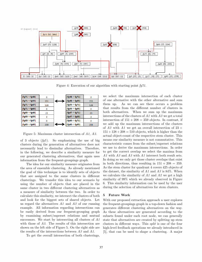
Figure 4: Execution of our algorithm with starting point fg71.

Figure 5: Maximum cluster intersection of A1, A3.

of 3 objects (fg5 ). So emphasizing the use of bigclusters during the generation of alternatives does notnecessarily lead to dissimilar alternatives. Therefore,in the following, we describe a similarity measure forour generated clustering alternatives, that again usesinformation from the frequent-groupings graph.

The idea for our similarity measure originates fromthe area of ensemble clustering. As already mentionedthe goal of this technique is to identify sets of objectsthat are assigned to the same clusters in differentclusterings. We transfer this idea to our scenario byusing the number of objects that are placed in thesame cluster in two different clustering alternatives asa measure of similarity between the two. In order tocalculate this similarity, we intersect the clusters of bothand look for the biggest sets of shared objects. Letus regard the alternatives A1 and A3 of our runningexample. All information regarding intersections canbe easily derived from our frequent-grouping graphby examining subset/superset relations and mutualsuccessors. We start by intersecting all clusters of A1with those of A3. The results of this intersection areshown on the left side of Figure 5. On the right side arethe results of the intersections between A3 and A1.

To get the overall intersection of both clusterings,

we select the maximum intersection of each clusterof one alternative with the other alternative and sumthem up. As we can see there occurs a problemthat results from the different number of clusters inboth alternatives. When we sum up the maximumintersections of the clusters of A1 with A3 we get a totalintersection of 151 + 208 = 359 objects. In contrast, ifwe add up the maximum intersections of the clustersof A3 with A1 we get an overall intersection of 23 +151 + 128 + 208 = 510 objects, which is higher than theactual object-count of the respective stem cluster. Thismeans our similarity measure is not commutative. Thischaracteristic comes from the subset/superset relationswe use to derive the maximum intersections. In orderto get the correct overlap we select the maxima fromA1 with A3 and A3 with A1 intersect both result sets.In doing so we only get those cluster overlaps that existin both directions, thus resulting in 151 + 208 = 359.As the stem cluster for quadrant 4 covers 425 objects ofthe dataset, the similarity of A1 and A3 is 84%. Whenwe calculate the similarity of A1 and A2 we get a highsimilarity of 99% which we already observed in Figure6. This similarity information can be used by the userduring the selection of alternatives for stem clusters.

5 Future Work

With our proposed extraction approach a user exploresthe frequent-groupings graph in a top-down fashion andgenerates different clustering alternatives on the way.As these alternatives are generated according to thesubsets found under each root node, we can generallystate that alternatives are created by splitting up stemclusters in different ways. This split is one of the fourhigh-level feedback operations we already introduced in[5], that can be used to shape a clustering. A major

37

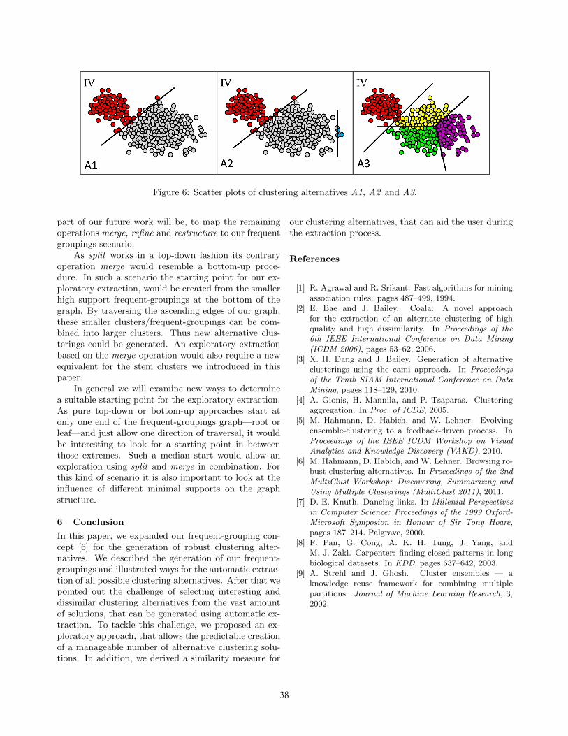
Figure 6: Scatter plots of clustering alternatives A1, A2 and A3.

part of our future work will be, to map the remainingoperations merge, refine and restructure to our frequentgroupings scenario.

As split works in a top-down fashion its contraryoperation merge would resemble a bottom-up proce-dure. In such a scenario the starting point for our ex-ploratory extraction, would be created from the smallerhigh support frequent-groupings at the bottom of thegraph. By traversing the ascending edges of our graph,these smaller clusters/frequent-groupings can be com-bined into larger clusters. Thus new alternative clus-terings could be generated. An exploratory extractionbased on the merge operation would also require a newequivalent for the stem clusters we introduced in thispaper.

In general we will examine new ways to determinea suitable starting point for the exploratory extraction.As pure top-down or bottom-up approaches start atonly one end of the frequent-groupings graph—root orleaf—and just allow one direction of traversal, it wouldbe interesting to look for a starting point in betweenthose extremes. Such a median start would allow anexploration using split and merge in combination. Forthis kind of scenario it is also important to look at theinfluence of different minimal supports on the graphstructure.

6 Conclusion

In this paper, we expanded our frequent-grouping con-cept [6] for the generation of robust clustering alter-natives. We described the generation of our frequent-groupings and illustrated ways for the automatic extrac-tion of all possible clustering alternatives. After that wepointed out the challenge of selecting interesting anddissimilar clustering alternatives from the vast amountof solutions, that can be generated using automatic ex-traction. To tackle this challenge, we proposed an ex-ploratory approach, that allows the predictable creationof a manageable number of alternative clustering solu-tions. In addition, we derived a similarity measure for

our clustering alternatives, that can aid the user duringthe extraction process.

References

[1] R. Agrawal and R. Srikant. Fast algorithms for miningassociation rules. pages 487–499, 1994.

[2] E. Bae and J. Bailey. Coala: A novel approachfor the extraction of an alternate clustering of highquality and high dissimilarity. In Proceedings of the6th IEEE International Conference on Data Mining(ICDM 2006), pages 53–62, 2006.

[3] X. H. Dang and J. Bailey. Generation of alternativeclusterings using the cami approach. In Proceedingsof the Tenth SIAM International Conference on DataMining, pages 118–129, 2010.

[4] A. Gionis, H. Mannila, and P. Tsaparas. Clusteringaggregation. In Proc. of ICDE, 2005.

[5] M. Hahmann, D. Habich, and W. Lehner. Evolvingensemble-clustering to a feedback-driven process. InProceedings of the IEEE ICDM Workshop on VisualAnalytics and Knowledge Discovery (VAKD), 2010.

[6] M. Hahmann, D. Habich, and W. Lehner. Browsing ro-bust clustering-alternatives. In Proceedings of the 2ndMultiClust Workshop: Discovering, Summarizing andUsing Multiple Clusterings (MultiClust 2011), 2011.

[7] D. E. Knuth. Dancing links. In Millenial Perspectivesin Computer Science: Proceedings of the 1999 Oxford-Microsoft Symposion in Honour of Sir Tony Hoare,pages 187–214. Palgrave, 2000.

[8] F. Pan, G. Cong, A. K. H. Tung, J. Yang, andM. J. Zaki. Carpenter: finding closed patterns in longbiological datasets. In KDD, pages 637–642, 2003.

[9] A. Strehl and J. Ghosh. Cluster ensembles — aknowledge reuse framework for combining multiplepartitions. Journal of Machine Learning Research, 3,2002.

38