Embed Size (px)
Citation preview

4 - 1© 2011 Pearson Education, Inc. publishing as Prentice Hall
44 ForecastingForecasting
PowerPoint presentation to accompany PowerPoint presentation to accompany Heizer and Render Heizer and Render Operations Management, 10e Operations Management, 10e Principles of Operations Management, 8ePrinciples of Operations Management, 8e
PowerPoint slides by Jeff Heyl

4 - 2© 2011 Pearson Education, Inc. publishing as Prentice Hall
What is Forecasting?What is Forecasting?
Process of predicting a future event
Underlying basis of all business decisions Production
Inventory
Personnel
Facilities
??

4 - 3© 2011 Pearson Education, Inc. publishing as Prentice Hall
Short-range forecast Up to 1 year, generally less than 3 months
Purchasing, job scheduling, workforce levels, job assignments, production levels
Medium-range forecast 3 months to 3 years
Sales and production planning, budgeting
Long-range forecast 3+ years
New product planning, facility location, research and development
Forecasting Time HorizonsForecasting Time Horizons

4 - 4© 2011 Pearson Education, Inc. publishing as Prentice Hall
Types of ForecastsTypes of Forecasts
Economic forecasts Address business cycle – inflation rate,
money supply, housing starts, etc.
Technological forecasts Predict rate of technological progress
Impacts development of new products
Demand forecasts Predict sales of existing products and
services

4 - 5© 2011 Pearson Education, Inc. publishing as Prentice Hall
Forecasting ApproachesForecasting Approaches
Used when situation is vague and little data exist New products
New technology
Involves intuition, experience e.g., forecasting sales on
Internet
Qualitative MethodsQualitative Methods

4 - 6© 2011 Pearson Education, Inc. publishing as Prentice Hall
Forecasting ApproachesForecasting Approaches
Used when situation is ‘stable’ and historical data exist Existing products
Current technology
Involves mathematical techniques e.g., forecasting sales of color
televisions
Quantitative MethodsQuantitative Methods

4 - 7© 2011 Pearson Education, Inc. publishing as Prentice Hall
Overview of Quantitative Overview of Quantitative ApproachesApproaches
1. Naive approach
2. Moving averages
3. Exponential smoothing
4. Trend projection
5. Linear regression
time-series models
associative model

4 - 8© 2011 Pearson Education, Inc. publishing as Prentice Hall
Set of evenly spaced numerical data Obtained by observing response
variable at regular time periods
Forecast based only on past values, no other variables important Assumes that factors influencing
past and present will continue influence in future
Time Series ForecastingTime Series Forecasting

4 - 9© 2011 Pearson Education, Inc. publishing as Prentice Hall
Trend
Seasonal
Cyclical
Random
Time Series ComponentsTime Series Components

4 - 10© 2011 Pearson Education, Inc. publishing as Prentice Hall
Components of DemandComponents of DemandD
eman
d f
or
pro
du
ct o
r se
rvic
e
| | | |1 2 3 4
Time (years)
Average demand over 4 years
Trend component
Actual demand line
Random variation
Figure 4.1
Seasonal peaks

4 - 11© 2011 Pearson Education, Inc. publishing as Prentice Hall
Persistent, overall upward or downward pattern
Changes due to population, technology, age, culture, etc.
Typically several years duration
Trend ComponentTrend Component

4 - 12© 2011 Pearson Education, Inc. publishing as Prentice Hall
Regular pattern of up and down fluctuations
Due to weather, customs, etc.
Occurs within a single year
Seasonal ComponentSeasonal Component
Number ofPeriod Length Seasons
Week Day 7Month Week 4-4.5Month Day 28-31Year Quarter 4Year Month 12Year Week 52

4 - 13© 2011 Pearson Education, Inc. publishing as Prentice Hall
Repeating up and down movements
Affected by business cycle, political, and economic factors
Multiple years duration
Often causal or associative relationships
Cyclical ComponentCyclical Component
0 5 10 15 20

4 - 14© 2011 Pearson Education, Inc. publishing as Prentice Hall
Erratic, unsystematic, ‘residual’ fluctuations
Due to random variation or unforeseen events
Short duration and nonrepeating
Random ComponentRandom Component
M T W T F

4 - 15© 2011 Pearson Education, Inc. publishing as Prentice Hall
MA is a series of arithmetic means
Used if little or no trend
Used often for smoothing Provides overall impression of data
over time
Moving Average MethodMoving Average Method
Moving average =∑ demand in previous n periods
n

4 - 16© 2011 Pearson Education, Inc. publishing as Prentice Hall
Form of weighted moving average Weights decline exponentially
Most recent data weighted most
Requires smoothing constant () Ranges from 0 to 1
Subjectively chosen
Involves little record keeping of past data
Exponential SmoothingExponential Smoothing

4 - 17© 2011 Pearson Education, Inc. publishing as Prentice Hall
Exponential SmoothingExponential Smoothing
New forecast = Last period’s forecast+ (Last period’s actual demand
– Last period’s forecast)
Ft = Ft – 1 + (At – 1 - Ft – 1)
where Ft = new forecast
Ft – 1 = previous forecast
= smoothing (or weighting) constant (0 ≤ ≤ 1)

4 - 18© 2011 Pearson Education, Inc. publishing as Prentice Hall
Common Measures of ErrorCommon Measures of Error
Mean Absolute Deviation (MAD)
MAD =∑ |Actual - Forecast|
n
Mean Squared Error (MSE)
MSE =∑ (Forecast Errors)2
n

4 - 19© 2011 Pearson Education, Inc. publishing as Prentice Hall
Common Measures of ErrorCommon Measures of Error
Mean Absolute Percent Error (MAPE)
MAPE =∑100|Actuali - Forecasti|/Actuali
n
n
i = 1

4 - 20© 2011 Pearson Education, Inc. publishing as Prentice Hall
Trend ProjectionsTrend Projections
Fitting a trend line to historical data points to project into the medium to long-range
Linear trends can be found using the least squares technique
y = a + bx^
where y= computed value of the variable to be predicted (dependent variable)a= y-axis interceptb= slope of the regression linex= the independent variable
^
4 - 21© 2011 Pearson Education, Inc. publishing as Prentice Hall
Seasonal Variations In DataSeasonal Variations In Data
The multiplicative seasonal model can adjust trend data for seasonal variations in demand

4 - 22© 2011 Pearson Education, Inc. publishing as Prentice Hall
Associative ForecastingAssociative Forecasting
Used when changes in one or more independent variables can be used to predict
the changes in the dependent variable
Most common technique is linear regression analysis
We apply this technique just as we did We apply this technique just as we did in the time series examplein the time series example

4 - 23© 2011 Pearson Education, Inc. publishing as Prentice Hall
Associative ForecastingAssociative ForecastingForecasting an outcome based on predictor variables using the least squares technique
y = a + bx^
where y= computed value of the variable to be predicted (dependent variable)a= y-axis interceptb= slope of the regression linex= the independent variable though to predict the value of the dependent variable
^

4 - 24© 2011 Pearson Education, Inc. publishing as Prentice Hall
Associative Forecasting Associative Forecasting ExampleExample
Sales Area Payroll($ millions), y ($ billions), x
2.0 13.0 32.5 42.0 22.0 13.5 7
4.0 –
3.0 –
2.0 –
1.0 –
| | | | | | |0 1 2 3 4 5 6 7
Sal
es
Area payroll

4 - 25© 2011 Pearson Education, Inc. publishing as Prentice Hall
Associative Forecasting Associative Forecasting ExampleExample
Sales, y Payroll, x x2 xy
2.0 1 1 2.03.0 3 9 9.02.5 4 16 10.02.0 2 4 4.02.0 1 1 2.03.5 7 49 24.5
∑y = 15.0 ∑x = 18 ∑x2 = 80 ∑xy = 51.5
x = ∑x/6 = 18/6 = 3
y = ∑y/6 = 15/6 = 2.5
b = = = .25∑xy - nxy
∑x2 - nx2
51.5 - (6)(3)(2.5)
80 - (6)(32)
a = y - bx = 2.5 - (.25)(3) = 1.75
4 - 26© 2011 Pearson Education, Inc. publishing as Prentice Hall
Associative Forecasting Associative Forecasting ExampleExample
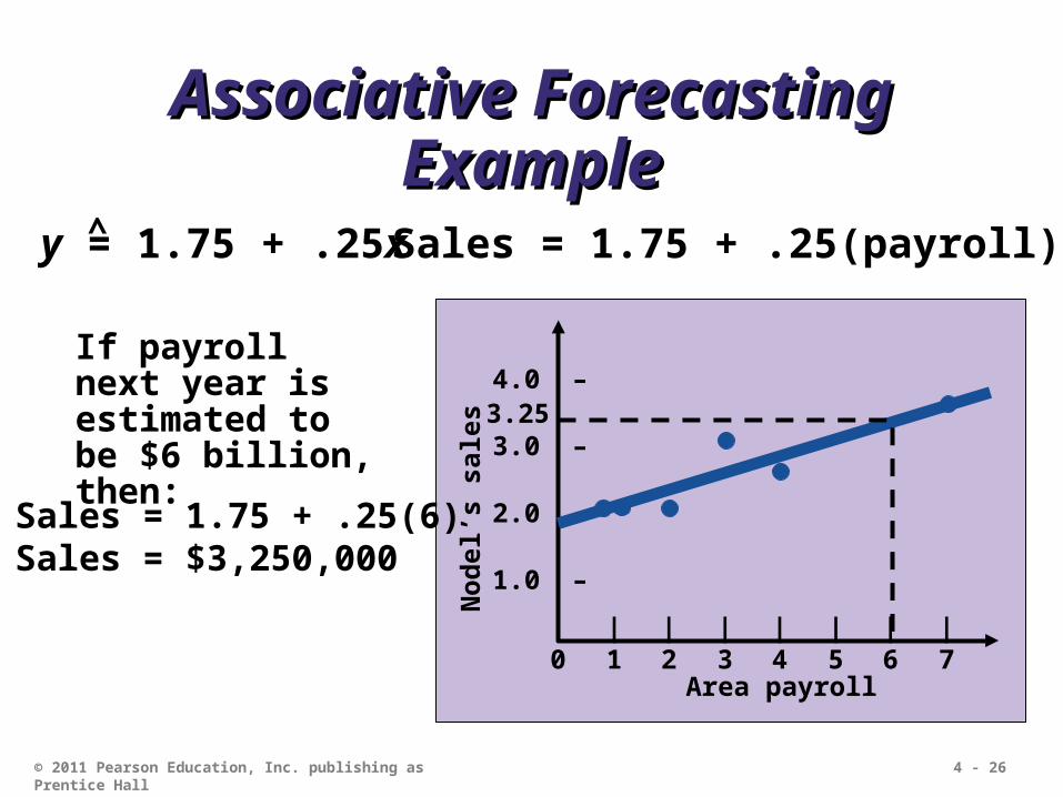
y = 1.75 + .25x^ Sales = 1.75 + .25(payroll)
If payroll next year is estimated to be $6 billion, then:
Sales = 1.75 + .25(6)Sales = $3,250,000
4.0 –
3.0 –
2.0 –
1.0 –
| | | | | | |0 1 2 3 4 5 6 7
No
del
’s s
ales
Area payroll
3.25

4 - 27© 2011 Pearson Education, Inc. publishing as Prentice Hall
Standard Error of the Standard Error of the EstimateEstimate
A forecast is just a point estimate of a future value
This point is actually the mean of a probability distribution
Figure 4.9
4.0 –
3.0 –
2.0 –
1.0 –
| | | | | | |0 1 2 3 4 5 6 7
No
del
’s s
ales
Area payroll
3.25

4 - 28© 2011 Pearson Education, Inc. publishing as Prentice Hall
Standard Error of the Standard Error of the EstimateEstimate
where y = y-value of each data point
yc = computed value of the dependent variable, from the regression equation
n = number of data points
Sy,x =∑(y - yc)2
n - 2

4 - 29© 2011 Pearson Education, Inc. publishing as Prentice Hall
How strong is the linear relationship between the variables?
Correlation does not necessarily imply causality!
Coefficient of correlation, r, measures degree of association Values range from -1 to +1
CorrelationCorrelation

4 - 30© 2011 Pearson Education, Inc. publishing as Prentice Hall
Correlation CoefficientCorrelation Coefficient
r = nxy - xy
[nx2 - (x)2][ny2 - (y)2]

4 - 31© 2011 Pearson Education, Inc. publishing as Prentice Hall
Correlation CoefficientCorrelation Coefficient
r = nxy - xy
[nx2 - (x)2][ny2 - (y)2]
y
x(a) Perfect positive correlation: r = +1
y
x(b) Positive correlation: 0 < r < 1
y
x(c) No correlation: r = 0
y
x(d) Perfect negative correlation: r = -1

4 - 32© 2011 Pearson Education, Inc. publishing as Prentice Hall
Coefficient of Determination, r2, measures the percent of change in y predicted by the change in x Values range from 0 to 1
Easy to interpret
CorrelationCorrelation
For the Nodel Construction example:
r = .901
r2 = .81

4 - 33© 2011 Pearson Education, Inc. publishing as Prentice Hall
Multiple Regression Multiple Regression AnalysisAnalysis
If more than one independent variable is to be used in the model, linear regression can be
extended to multiple regression to accommodate several independent variables
y = a + b1x1 + b2x2 …^
Computationally, this is quite Computationally, this is quite complex and generally done on the complex and generally done on the
computercomputer

4 - 34© 2011 Pearson Education, Inc. publishing as Prentice Hall
Multiple Regression Multiple Regression AnalysisAnalysis
y = 1.80 + .30x1 - 5.0x2^
In the Nodel example, including interest rates in the model gives the new equation:
An improved correlation coefficient of r = .96 means this model does a better job of predicting the change in construction sales
Sales = 1.80 + .30(6) - 5.0(.12) = 3.00Sales = $3,000,000


![[PPT]Heizer/Render 11e - OER University - Anvari.Netcbafaculty.org/Operations_Management/hr_om11_ch09.ppt · Web viewTitle Heizer/Render 11e Subject Chapter 9 - Layout Strategies](https://img.pdfslide.net/doc/110x75/5b067bef7f8b9abf568d176c/pptheizerrender-11e-oer-university-viewtitle-heizerrender-11e-subject-chapter.jpg)


![[Jay Heizer, Barry Render]Operations Management 10e](https://img.pdfslide.net/doc/110x75/55cf8e81550346703b92d9f3/jay-heizer-barry-renderoperations-management-10e-56427fb5ecb7b.jpg)