4 64 35 5 TG 547JANUARY 1964

AQ4

ANALYSIS of SATELLITE TIME DATA

_) by

W. H. GUIER

THE JOHNS HOPKINS UNIVERSITY

APPLIED PHYSICS LABORATORYSILVER SPRING, MARYLAND

NOperting~ under Contruett NOw 62..0604--c with the Bureau of Naval Weapons, Deportment of the Navy

TG 547 1(J A NOM 4)

COPY NO.

ANALYSIS of SATELLITE TIME DATA

by "",b

W. H. GUIER.

ct Nofl Dl-I

u z1iK

APPLIC8 P NAV ,K LAGORAIAIt

ANALYSIS OP SATELLITE TIME DATA

W. H. Quier ra

Satellites 1961 01, 1961 a11, and 1962 5P1 are instrumented to

supply time data as well as doppler data. Satellite time markers are/(generated in these satellites by counting down' the satellite's stable

oscillator and producing a unique modulating on the doppler carriers each

time a fixed nwmber of oscillator cycles have occurred. The TRAOET doppler

receiving stations are equipped to recognize this modulation and to

automatically punch (on the same paper tape that doppler data is punched)

the station's time (WWV) at which this special modulation is received.

After appropriate calibration, this time data can serve as a secondary

time standard. This report presents the information required to recognize

and process satellite time data and to determine the WWV time at which

the satellites transmitted satellite time markers.

The" report is divided into two sections. first section presents

the basic eouations that connect the satellite transmitter frequency, the

station s satellite time data, and the times that the satellites transmitted

the time markers. The second section presents the information required to

recognize, re-format, and reduce the experimental satellite time data to a

form appropriate to the theory presented in the first section.

A7I/

SZNW SWIM.ng Ma4'%1a

-2-

I. DERIVATION OF EQUATIONS FOR SATLLITE TBIE

This section presents the equations connecting the satellite's

oscillator frequency, the stations' data when the satellite transmitted

time markers, and inferred values for the times when time markers are

transmitted relative to a chosen standard of time. The section is

divided into three sub-sections. The first sub-section presents the

notation for important quantities which are used throughout this report.

The second sub-section presents the equations to determine the absolute

frequency of the satellite as a function of time. The third sub-section

presents one method for statistically inferring when the satellite

transmitted time markers. Also included in the third section is a

suggestion for a simplified equation to predict into the future the times

that satellite time markers are transmitted for station alert purposes.

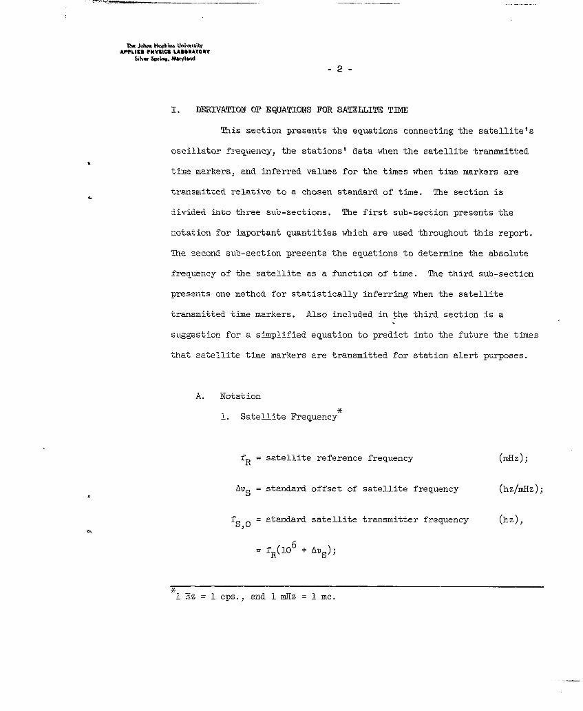
A. Notation

*L. Satellite Frequency

f, = satellite reference frequency (mHz);

AVS = standard offset of satellite frequency (hz/mHz);

fso = standard satellite transmitter frequency (hz),

= f R (1 6 + A S);

! Hz =1 cps., and 1 mHz = 1 inc.

ArrEo PR" LAVI&TOKY

3-

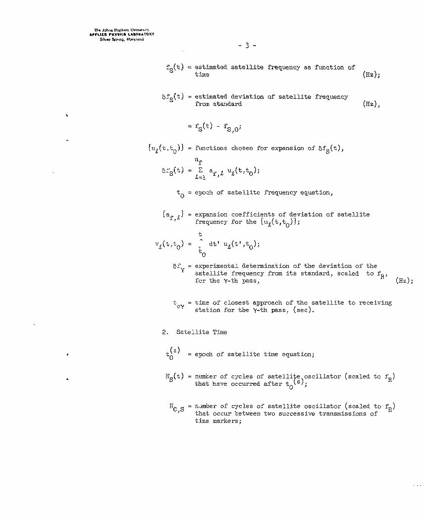
fS(t) = estimated satellite frequency as function oftime (Hz)

5fs(t) = estimated deviation of satellite frequencyfl-om standard (Hz),

f S (t ) - f . ;

u (tt)} tuinctions chosen for expansion of 5fs(t),

n f

>(t) = - f'L J(t,tO);

t = epoch of satellite frequency equation,

(a- = expansion coefficients of deviation of satellitefrequency for the [u£(t,to)1;

= t%(t' o) k dt' u "t ,to)

000

5 -= experimental determination of the deviation of thesatellite frequency from its standard, scaled to fR

for the y-th pass, (Hz);

t = time of closest approach of the satellite to receivingstation for the y-th pass. (sec).

2. Satellite Time

(s)- epoch of satellite time equation;

?1(t 0 tave ocuIe after

= ntLber of cycles of satellite oscillator (scaled to f,)that have occurred afte toS);

N CS = n~mber of cycles of satellite oscillator (scaled to fR)

that occur between two successive transmissions of

time markers;

APULIO PwtNc LAUtUA RY

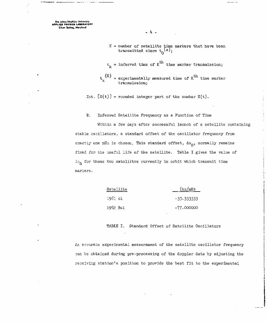
K = nmer of satellite Viqle markers that have beentransmitted since t0ks;

t k = inferred time of K th time marker transmission;

(E) = experimentally measured time of K t h time markertransmission;

Int. [X(t)] = rounded integer part of the number X(t).

B. T-nferred Satellite Frequency as a Function of Time

WitInin a few days after successful launch of a satellite containing

stable oscillators, a standard offset of the oscillator frequency fromexactly one mHz is chosen. This standard offset, A normally remains

:N-ed fo r the usefuI life of the satellite. Table I gives the value of

u for those two satellites currently in orbit which transmit time

markers.

Satel - ite (hz/mHz

1961 o, -35.333333

1962 i -77.000000

TITB I. Standard Offset of Satellite Oscillators

An acrate exrerimental measurement of the satellite oscillator frequency

2- be obtained during pre-processing of the doppler data by adjusting the

receiving stations nosition to provide the best fit to the experimental

&Not4 Sptk, omit". '~

doppler data. This, experimental measur-ement of' the satellite oscillator

:ftreicy for the 'y-thi pass is usually scaled to some convenient reference

freuenyf Rand is given as a corre-ction term, 5f.Y otesadr

satellite frequency, f f R(l00 + AUS).

Consequently, letting the time of' closest approach for the

'Y-th pass, t Ibe the timte associated with the experimental measurement

of frequency, 5fYit can be seen that the deviation of the satellite

fr~eauency from its standard freauency, 5f (t), cnb ietyifre

from the experimental dt, [5f Y I Let the deviation of' the satellite

frequency be parameterized in the form:

.,here the uLtt)are known functions of' the time and chosen to

accurately represent the variations of' the satellite oscillator

freauency as a function of' the time t', and the f'requency epoch, t 0

Choosing a convenient epoch; to.? for equation (1.1), a least squares

dete-rinto - 'o th expansion coefficients, [af 9]:

*1961 rirl data indicates that for active temperature controlled satellite

oscifLItors, u, 1 and u2 (t,t 0 ) = t - to are adequate for parameterizing

the variations of' the satellite frequency, so long as the ambient satellite

temerature remains within the control range.

(1)!Orboit imgroviement Program", PPL/JHU Report TG-40l.

APLIEUR PHi= LANORA1OmY

6-

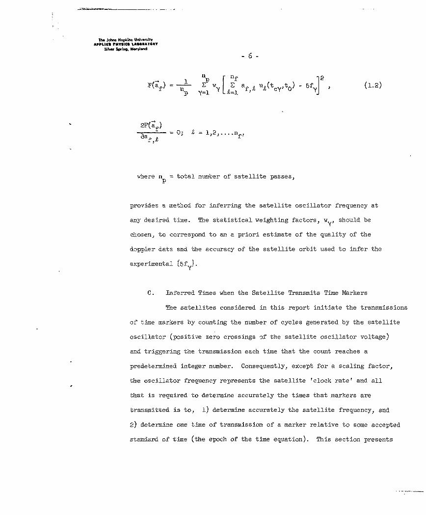
11 p f ] 2,%fj-~L~ w , u (to ,t 0) - sf ,(1.2)

2F('af)

=F (af ; L = !,2, .... no

where n total number of satellite passes,0

provides a method for inferring the satellite oscillator frequency at

any desired time. The statistical weighting factors, w, should be

chosen, to correspond to an a priori estimate of the quality of the

doppler data and the accuracy of the satellite orbit used to infer the

exrperimental [f }.

C. inferred Times fnen the Satellite Transmits Time Markers

Me satellites considered in this report initiate the transmissions

of time markers by counting the number of cycles generated by the satellite

oscillator (positive zero crossings of the satellite oscillator voltage)

and triggering the transmission each time that the count reaches a

predetermined integer number. Consequently, except for a scaling factor,

the oscillator frequency represents the satellite 'clock rate' and all

that is reouired to determine accurately the times that markers are

transmitted is to, 1) determine accurately the satellite frequency, and

2) determine one time of transmission of a marker relative to some accepted

stadard of time (the epoch of the time equation). This section presents

APFUIE rMI"W LAMIAte "RY

7-

the infoLmation recuiUred to deteriine the scaling factor for the clock

rate and the eauations to determine the time of transmission of one

time nmarker, given experimental measurements of the times of transmission

of time markers relative to an accepted time standard. In addition,

this section presents the equations necessary to check the station

clock of any receiving station. Finally, this section presents one

foin of a simplified eauation that is convenient to use for extrapolating

ma-w-ker trapsmission times into the future to an accuracy sufficient for

station alert pupposes.

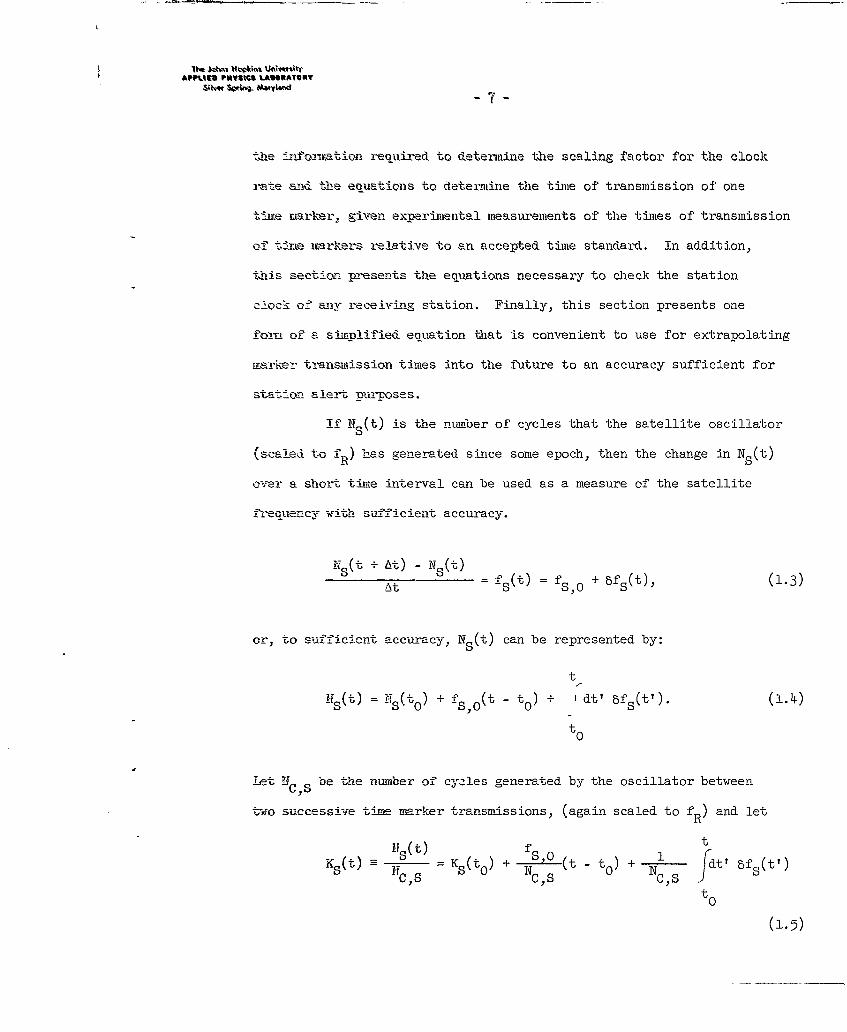
if Ns(t) is the nunber of cycles that the satellite oscillator

(scaled to -R) has generated since some epoch, then the change in Ns(t)

over a short time interval can be used as a measure of the satellite

frequency with sufficient accuracy.

S t t) - = fs(t) = o, + 5fs(t)' (1.3)

or, to sufficient accuracy, Ns(t) can be represented by:

t

7s(t ) = 1s(to) + fs o(t - t0 ) + I dt' 5fs(t'). (1.4)

to

Let FT be the number of cycles generated by the oscillator between

two successive time marker transmissions, (again scaled to f R) and let

K3 (tN) = (t) -Ks(tO) + '- (t - to) +N t, fs(t')

C;S C,'S CISto0

AIPPU~t PIN U~lcS LUI UUWllI

-8-

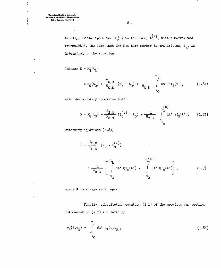
Finally, if the epoch for Ns(t ) is the tile" to, that a marker was

transmaitted, the time that the Kth time marker is transmitted, tk, is

dete rined by the equation:

Tnteger K =sWt)to

= YI,+(ttO ) + f~ dr' 5fs W), (1.6A)

With the boundary condition that:

t(s)

0 Y 0 ) + - cs ( - to) + 1Ncs dt' fs(t'). (1.6B)

to

Comi-ning eauations (1.6),

K -S.0 - U(S)K --' i~- (t

(S)

Fk to

~ L at 5f(tr)- t dt' bfs(t') 17

where K is always an integer.

Finally, substituting equation (1.1) of the previous sub-section

into equation (1.7),and letting:

t

vf(t;to) = dt' V(t,to), (1.8A)

to

-9-

then

K , (tk-t~) + 1 Z a vY( - v pt 0s,t0 (1. 8B)

11S IsQ0,CS A=i f.A ,k0) V

Table I in Section I.A. listed values of Av from which f siocan be

calculated. Table I!, given below, lists the values of N C 5 for the three

1 telites of- interest in this report. Assuming that the frequency epoch,

has been chosen and the values of the frequency expansion coefficients,

haebeen inferred -From dop-Pler data as discussed in section l.A.,

tioiere remain in eauations (1.8) only three possible unknowrns: K, tk or tsk' 0

it can be seen That if any two of these three are known, the third can be

found 'ron~ the above eouations. Three cases are now discussed, the case

ninber danding upon wehich of the three variables is considered unknown.

SatelIlite N C'sat 3 mHz.

061, ol 100712448

2961 a67092480

2962 =I 268435456

jbIE TT. Nainber of Oscillator Cycles Occurring between Time Markers

Cas 1: Lne Niumber of the Time Marker, K, is Unknown.

From the numfoers given in Tables I and II, it can be seen that

two time ma--rkers can not occur more frequently than about every 20 seconds.

Consequently-, given an approximate time of transmission of a time marker,

tE and an approximate value for the time of the zeroth time marker

AFVPLION PP"M"I LAMMA1URY

- 10 -

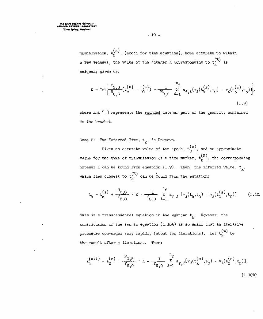
transmission, t(s), (epoch for time equation), both accurate to within

a few seconds, the value of the integer K corresponding to t (E) is

umiquely given by:

Intr f4 (t(E) - t(s)) + 1 Z' f(v 2 (t(E),to) - t

(1.9)

Ihere Tn i ] represents the rounded integer part of the quantity contained

in the bracket.

Case 2: The inferred Time, tk, is Unknown.

Given an accurate value of the epoch, t0s)", and an approximate

value for the time of transmission of a time marker, t(E), the corresponding

integer K can be found from equation (1.9). Then, the inferred value, tk,

which lies closest to t, can be found from the equation:

= = t(S)o + NO .fo K - Z 1 af, [ve(tktO)- e (t~s),to)] (l.lO,

This is a traunscendental equation in the unknown t However, the

contribution of the su to equation (l.lOA) is so small that an iterative

prccedure converges very rapidly (about two iterations). Let t(m) bek

the result after m iterations. Then:

J±)_N K- - nf-

( ts) 1 f [(t(m)t (S)

k 0 s~ 0so21a ~~kO--'S,O ,(0 l

(1 ..10B )

APPUfO PMtrnC L&AU@&ATRY

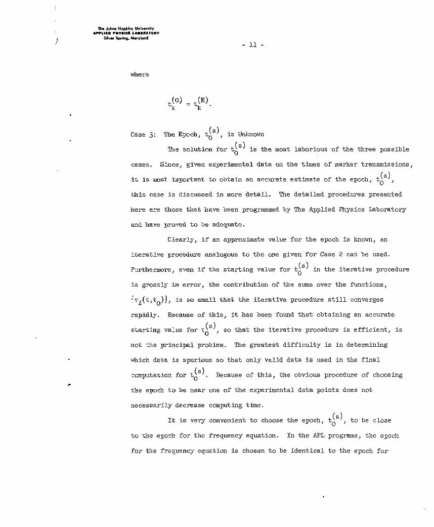
where

40) - t(E)k k"

Case 3: The Epoch, t(s) is Unknown0'

The solution to)- is the most laborious of the three possible

cases. Since, given experimental data on the times of marker transmissions,

it is Most inportant to obtain an accurate estimate of the epoch, toS)

dhis case is discussed in more detail. The detailed procedures presented

here are those that have been programmed by The Applied Physics Laboratory

and have proved to be adeauate.

Clearly. if an approxinate value for the epoch is known, an

iterative orocedue analogous to the one given for Case 2 can be used.

a uLhe--_lore, eN n if the starting value for tS) in the iterative procedure

is grossly in error, the contribution of the suns over the functions,

ivj(-tto is so small that the iterative procedure still converges

rapidly. Because of this, it has been found that obtaining an accurate

_(s)starting value for -O . so that the iterative procedure is efficient, is

not che orincipal problem. The greatest difficulty is in determining

which data is sourious so that only valid data is used in the finalco-mwo~uat, -r P-r_(s).

o _ptaticn for 0 Because of this, the obvious procedure of choosing

the epoch to be near one of the experimental data points does not

necessarily decrease computing time.

It is very convenient to choose the epoch, t(S) to be close

to the ecoch for the frequency equation. In the APL programs, the epoch

for the frequency equation is chosen to be identical to the epoch for

APPLIEm PN4YItcS LASRATURY

- 12 -

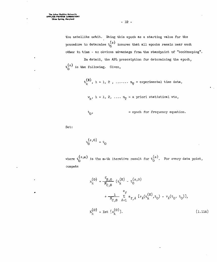
the satellite orbit. Using this epoch as a starting value for the

procedre to determine to)insures that all epochs remain near each

other in tive - an obvious advantage from the standpoint of "booldeeping".

i detail, the APL prescription for determining the epoch,

t(s) is the following. Given,

t k , k = 1: 2 . ....... n2 = experimental time data,

'k, k = 1) 2 ..... n = a priori statistical wts,

to; = epoch for frequency equation.

Set:

0 0

,where,(n) is the r-th iterative result for t(S). For every data point,

*cmpute

NC S -k 0

n_

N a fI [v,(tkE),to) - vI(to, t0)],NCS Y'=!

T(o) rx(O) I.11A

The JO"Nis nestAPM.UEC PIAM LABORATOmY

- 13 -

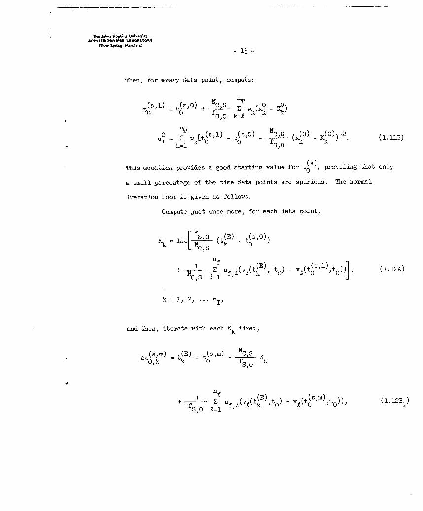
Then, for every data poinit, compute:

t(s,1) (So) +I 0N'0 fs,o k-- "

= T I p -t(s0o) C ) (0) _tK(o)(11 ki1k 0 fS' xi

SfsS0

This equation provides a good starting value for to providing that only

a small percentage of the time data points are spurious. The normal

iteration loop is given as follows.

Compute just once more, for each data point,

= ItE * (1 E) - (sO))K ! nt RI. L

i n f (E]V~(.1+ E a..(v(t(E) to- v(t(S )to ) (1.12A)CS =k 0 0

k = ! 2, .... n T

and then. iterate with each Kk fixed,

,..s~i)_ (E) - (s,m)-Nc10,k = k 0 fs o

n,

S E afI v(tt (E ) Ve5t0 '),t 0 )), (1.12B-S,O o =lI

&AlPPUiS PNtt~t3 LASSUAmm~y5pi'. N - 14 -

11TE 't At t( s m)

- s0k _ (1.12B2 )

k=!

2 k=l%i-I (1.12B3 )

E w

k=l

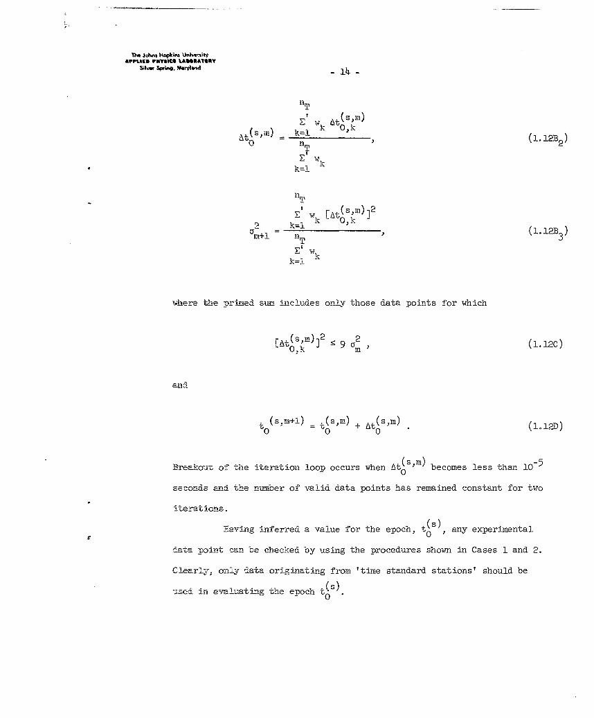
izhere the prined suim includes only those data points for which

r ts,.)l 2 ~ (1.12C)" O.Lk - a

(s,+-)= (s,m) + At(sm) (1.12D)0 o

Breakou of the iter-ation loop occurs when t(sm) becomes less than 10-5

seconds and the number of valid data points has remained constant for two

iterations.

saving inferred a value for the epoch, t(s), any experimental

data point can be checked by using the procedures shown in Cases 1 and 2.

Clearly; only data originating from 'time standard stations' should be

ased -in evaluati-ng the epoch t( S )

0)

ohn ~s "OP~ns UnIewit*APPLIED PNMStC8 LAIORMATURY

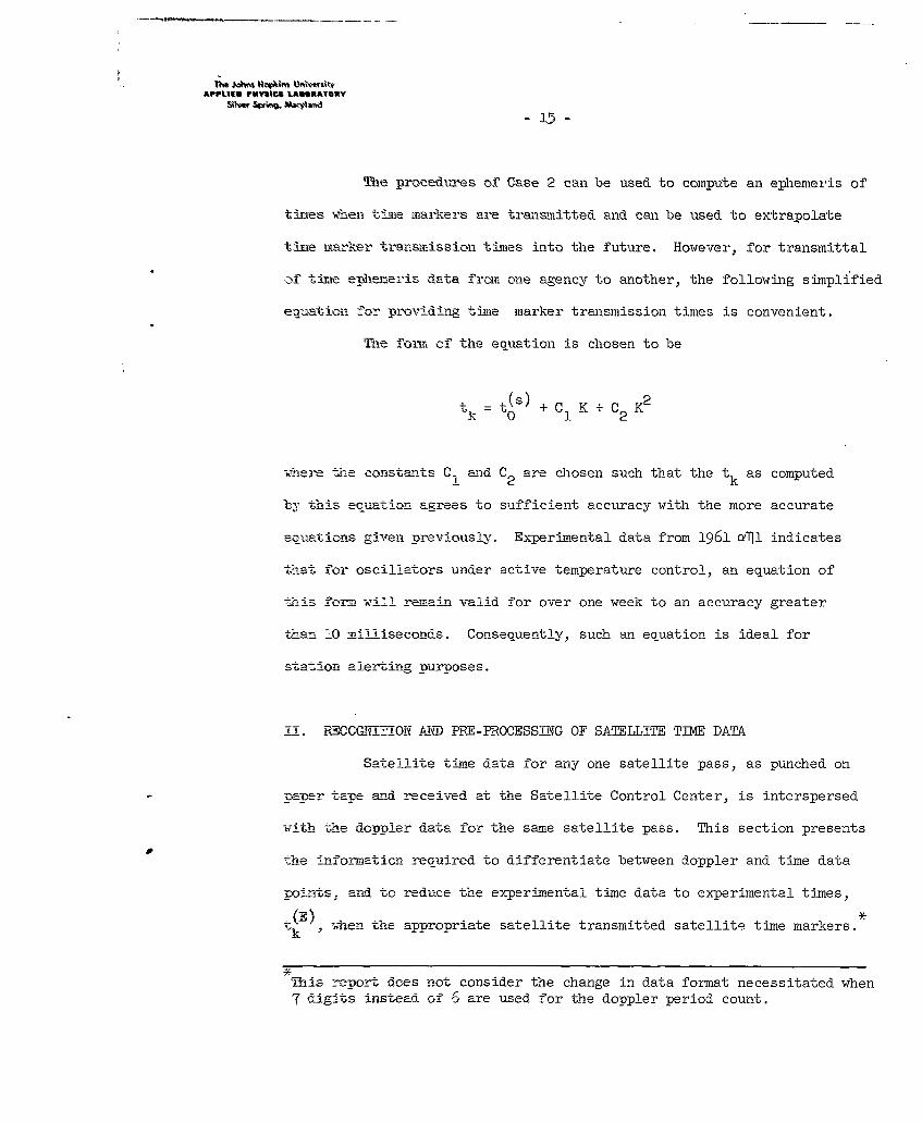
The procedures of Case 2 can be used to compute an ephemeris of

times N hen time markers are transmitted and can be used to extrapolate

time marker transmission times into the future. However, for transmittal

of time ephemeris data from one agency to another. the following simplified

equation for providing time marker transmission times is convenient.

The form of the equation is chosen to be

t(s) + C K + C lek 0 1 2

Where the constants C Iand C2 are chosen such that the t k as computed

b5" this equation agrees to sufficient accuracy with the more accurate

equations given previously. Exsperimental data from 1961 ai indicates

that for oscillators under active temperature control, an equation of

this form will remain valid for over one week to an accuracy greater

than 10 milliseconds. Consequently, such an equation is ideal for

station aertina pur-oses.

I. _ECOGCIHTON AED PRE-PROCESSING OF SATELLITE TEME DATA

Satellite time data for any one satellite pass, as punched on

aoer taoe and received at the Satellite Control Center, is interspersed

-iththe doppler data for the same satellite pass. This section presents

the __nformation required to differentiate between doppler and time data

_o-nts, and to reduce the experimental time data to experimental times,

(E)*4k , when the appropriate satellite transmitted satellite time markers.

This report does not consider the change in data format necessitated when7 digits instead of 6 are used for the doppler period count.

The lJohr How*ins UnivesitAPPLIEO PNY3 CS LASONATOT

Wv Spnrg, MVAtnd-16-

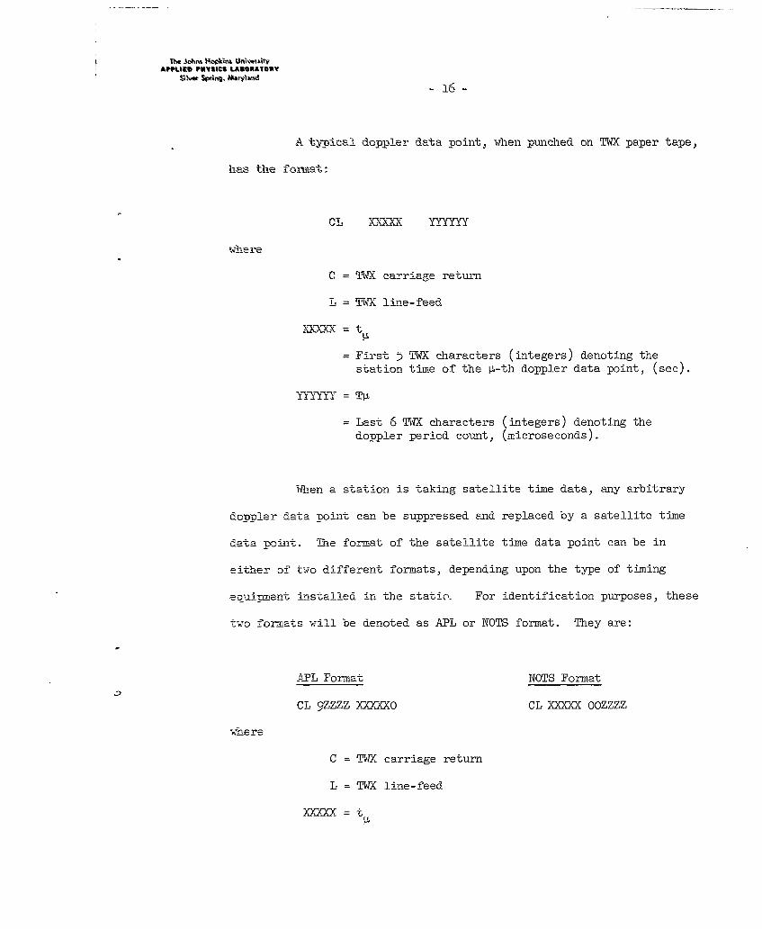
A typical doppler data point, when punched on TWX paper tape,

has the format:

CL X- r YYY

where

C = TWX carriage return

L = TWX line-feed

=t

= First 5 TWX characters (integers) denoting the

station time of the P-th doppler data point, (sec).

YY = T

= Last 6 TWX characters (integers) denoting thedoppler period count, (microseconds).

!%Rien a station is taking satellite time data, any arbitrary

doppler data point can be suppressed and replaced by a satellite time

data noit. The format of the satellite time data point can be in

either of- two different formats, depending upon the type of timing

eauarment installed in the statio. For identification purposes, these

two formats will be denoted as APL or NOTS format. They are:

APL Format NOTS Format

CL 9ZZZZ XO=O[O CL XXXXX OOZZZZ

-where

C = TWrX carriage return

L = TWX line-feed

X2000 = t

The Johm Hoi Unv"SAAPPLIED PN#tC% LABORATORY

17-

(Format cont'd.)

5 5 TWX characters (integers) giving the integer partwhen the satellite time mark is received, (see).

ZZZ = AT

= 4 TWX characters (integers) giving one correctionto be applied to t (tenths of milliseconds).

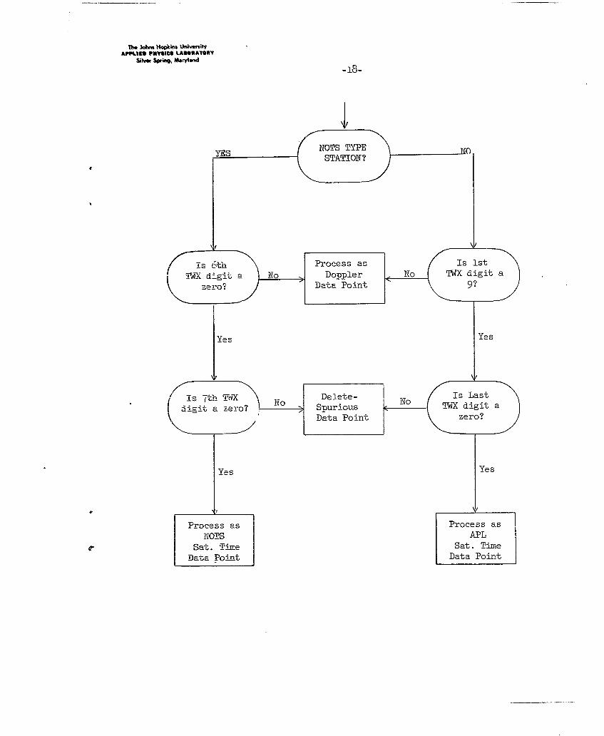
With either format a satellite time data point can be uniquely

identified when interspersed with doppler data because the TWX 9 in the

APL forimat and the first 1%X 0 (zero) in the NOTS format are illegal

characters for a doppler point. The following flow chart is an

example of a testing network to correctly identify each data point.

Upon identification of a satellite time data point, the

IWX C and L should be deleted, the remaining 11 TWX digits appropriately

uiracked. and transformed from BCI to the two floating point numbers.

= integer part of satellite time in seconds

AR correction for satellite time in units of 10 4

seconds.

Thie reconstruction of the time (WWV) that the satellite

transmitted a marker is given below. This reconstruction also depends

upon the ty-pe of station equipment (APL or NOTS) and, if obtained from

.APL ty-ne equipment, further depends upon the satellite transmitting

the time marker.

Doe Johns Hopkis ni MtyqAwt.1g. FMIAICS LABORATORY

Shm Sprkq, Mbtyland-

T-hX digrit a No Doppler No TWX digit a

Is -7thn ThX No Delete- N sLs

Process as Process asNOTS APL

Sat. Tir Sat. TimeData Point Data Point

APPLIED PHYSIC& LABORATORY

-19-

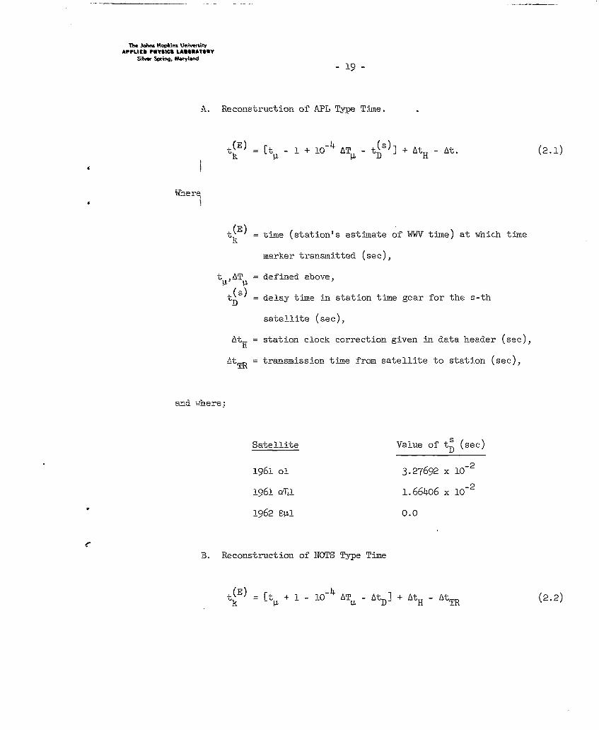
A. Reconstruction of A.PL Type Time.

4(E) - -4 AT- t(s)]i + AtH At. (2.1)tk p 0DH

14Whe re,

t(E k ime (station's estimate of WWV time) at which time

marker transmitted (sec),

tA.T = de finL-ed above,

(s) =delay time in station time gear for the s-th"D

satellite (see),

At.= station clock correction given in data header (sec),

L'tR = transmission time from satellite to station (sec),

and irhere;

S at e Ii t e Value of ts (see)

1061 ol 3.27692 x 10 2

i061 aF11 1.664jo6 x 10-2

i962 Bpi 0.0

B. Reconstruction of NOTS Type Time

t.(E) = rt + 1 _ 10- AT - t + At -At(2)

k ~ D H TR(2)

it* Johns HopkinsI Un~vetityAPPUE PYIICS LA8SUATORY

- 20-

where

t (E ) = tine (station's estimate of WWV time) at which time

marker transmitted by satellite, (sec),

t. , T = defined above,

AtH = station clock correction given in data header, (sec),

At = NOTS station delay time

6t = transmission time from satellite to station, (sec).TR b

Ecuations (2.1) and (2.2) define t(E) which is the stations best estimatek

of the time (1,AAF) that a satellite time mark is transmitted from the

satellite. Tyoically, from one to fifty such times can be received

during a single pass. Currently tD for the NOTS type time is zero.

TMe Johns H~okns UnivesiityAPPLIED PMYSWS LASGRATORY

Initial distribution of this document has been

made in accordance with a list on file in the Technical

Reports Group of The Johns Hopkins University, Applied

Physics Laboratory.