4. Coagulation, Precipitation, and Metals Removal

4.1. Introduction

Coagulation is a unit process used for removing colloids and other suspended particles from

water and wastewater. It may be employed as source treatment for the removal of contaminants

such as metals, within the treatment train, or with filtration as a polishing step. Coagulation

destabilizes colloidal particles by charge neutralization and promoting collisions between

neutralized particles, resulting in cohesion, floc growth, and eventual sedimentation and

filtration. This chapter considers the principles of the coagulation process, coagulant properties,

coagulation equipment, laboratory determinations for coagulant selection, and case studies. It

also includes removal technologies for heavy metals of frequent concern.

4.2. Coagulation

Colloids are particles within the size range of 1 nm (10 − 7 cm) to 0.1 nm (10 − 8 cm). These

particles do not settle out on standing and cannot be removed by conventional physical treatment

processes. Colloids present in wastewater can be either hydrophobic or hydrophilic. The

hydrophobic colloids (clays, etc.) possess no affinity for the liquid medium and lack stability in

the presence of electrolytes. They are readily susceptible to coagulation. Hydrophilic colloids,

such as proteins, exhibit a marked affinity for water. The absorbed water retards flocculation and

frequently requires special treatment to achieve effective coagulation. 1

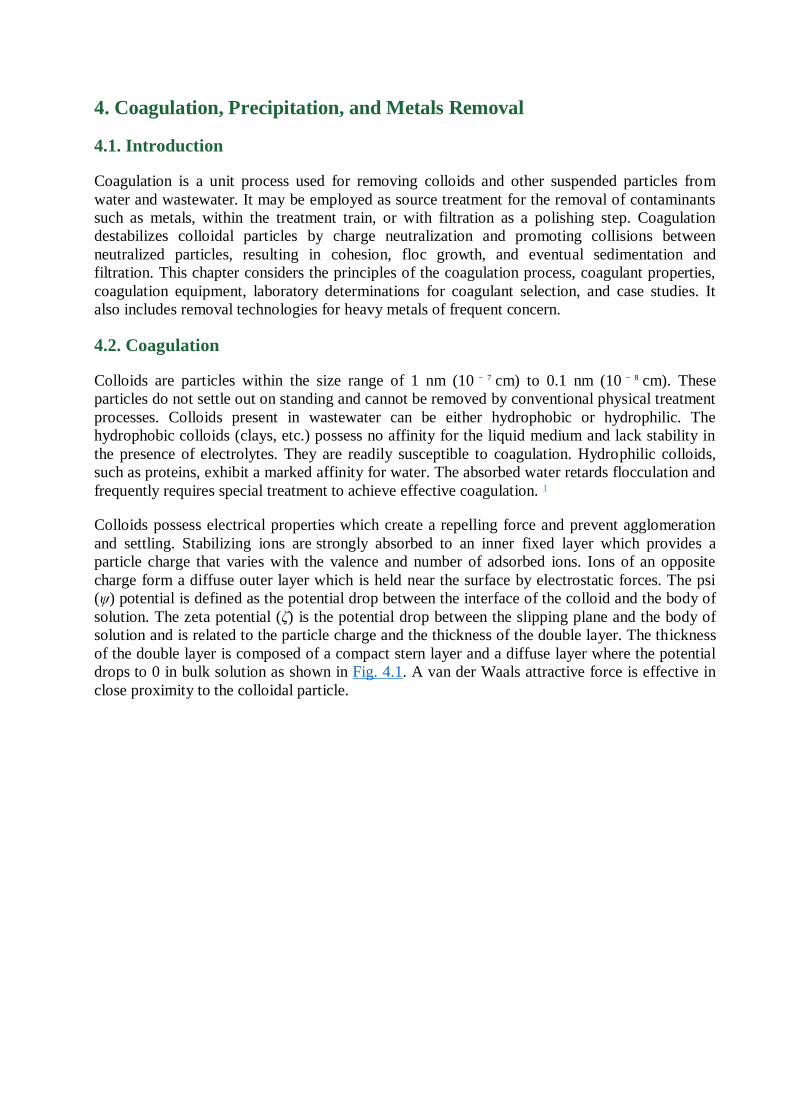
Colloids possess electrical properties which create a repelling force and prevent agglomeration

and settling. Stabilizing ions are strongly absorbed to an inner fixed layer which provides a

particle charge that varies with the valence and number of adsorbed ions. Ions of an opposite

charge form a diffuse outer layer which is held near the surface by electrostatic forces. The psi

(ψ) potential is defined as the potential drop between the interface of the colloid and the body of

solution. The zeta potential (ζ) is the potential drop between the slipping plane and the body of

solution and is related to the particle charge and the thickness of the double layer. The thickness

of the double layer is composed of a compact stern layer and a diffuse layer where the potential

drops to 0 in bulk solution as shown in Fig. 4.1. A van der Waals attractive force is effective in

close proximity to the colloidal particle.

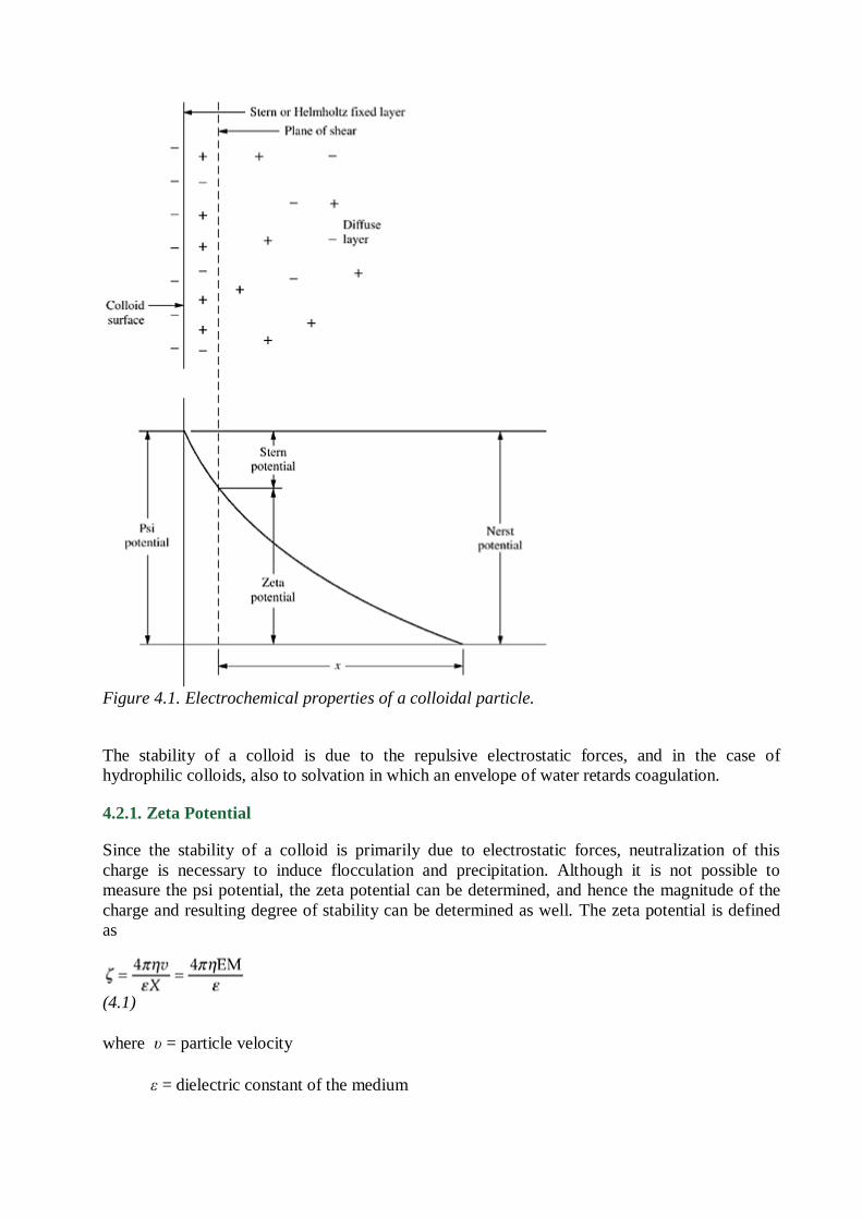
Figure 4.1. Electrochemical properties of a colloidal particle.

The stability of a colloid is due to the repulsive electrostatic forces, and in the case of

hydrophilic colloids, also to solvation in which an envelope of water retards coagulation.

4.2.1. Zeta Potential

Since the stability of a colloid is primarily due to electrostatic forces, neutralization of this

charge is necessary to induce flocculation and precipitation. Although it is not possible to

measure the psi potential, the zeta potential can be determined, and hence the magnitude of the

charge and resulting degree of stability can be determined as well. The zeta potential is defined

as

(4.1)

where υ = particle velocity

ε = dielectric constant of the medium

η = viscosity of the medium

X = applied potential per unit length of cell

EM = electrophoretic mobility

For practical usage in the determination of the zeta potential, Eq. (4.1) can be re -expressed:

(4.2)

where EM = electrophoretic mobility, (μm/s)/(V/cm).

At 25ºC, Eq. (4.2) reduces to

(4.3)

The zeta potential is determined by measurement of the mobility of colloidal particles across a

cell, as viewed through a microscope. 2 , 3 Several types of apparatus are commercially available

for this purpose. A recently developed Lazer Zee meter does not track individual particles, but

rather adjusts the image to produce a stationary cloud of particles using a rotating prism

technique. This apparatus is shown in Fig. 4.2. The computations involved in determining the

zeta potential are illustrated in Example 4.1.

Example 4.1.

In a electrophoresis cell 10 cm in length, grid divisions are 160 µm at 6 × magnification.

Compute the zeta potential at an impressed voltage of 35 V. The time of travel between grid

divisions is 42 s and the temperature is 20ºC.

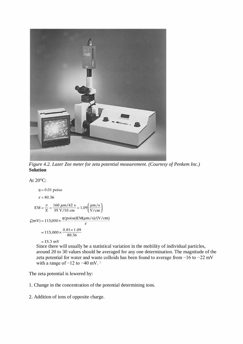
Figure 4.2. Lazer Zee meter for zeta potential measurement. (Courtesy of Penkem Inc.)

Solution

At 20°C:

Since there will usually be a statistical variation in the mobility of individual particles,

around 20 to 30 values should be averaged for any one determination. The magnitude of the

zeta potential for water and waste colloids has been found to average from −16 to −22 mV

with a range of −12 to −40 mV. 3

The zeta potential is lowered by:

1. Change in the concentration of the potential determining ions.

2. Addition of ions of opposite charge.

3. Contraction of the diffuse part of the double layer by increase in the ion concentration in solution.

Since a vast majority of colloids in industrial wastes possess a negative charge, the zeta potential

is lowered and coagulation is induced by the addition of high-valence cations. The precipitating

power of effectiveness of cation valence in the precipitation of arsenious oxide is

Optimum coagulation will occur when the zeta potential is zero; this is defined as the isoelectric

point. Effective coagulation will usually occur over a zeta potential range of ±0.5 mV.

4.2.2. Mechanism of Coagulation

Coagulation results from two basic mechanisms: perikinetic (or electrokinetic) coagulation, in

which the zeta potential is reduced by ions or colloids of opposite charge to a level below the van

der Waals attractive forces, and orthokinetic coagulation, in which the micelles aggregate and

form clumps that agglomerate the colloidal particles.

The addition of high-valence cations depresses the particle charge and the effective distance of

the double layer, thereby reducing the zeta potential. As the coagulant dissolves, the cations

serve to neutralize the negative charge on the colloids. This occurs before visible floc formation,

and rapid mixing which ―coats‖ the colloid is effective in this phase. Microflocs are then formed

which retain a positive charge in the acid range because of the adsorption of H +. These

microflocs also serve to neutralize and coat the colloidal particle. Flocculation agglomerates the

colloids with a hydrous oxide floc. In this phase, surface adsorption is also active. Colloids not

initially adsorbed are removed by enmeshment in the floc.

Riddick 3 has outlined a desired sequence of operation for effective coagulation. If necessary,

alkalinity should first be added. (Bicarbonate has the advantage of providing alkalinity without

raising the pH.) Alum or ferric salts are added next; they coat the colloid with Al 3 + or Fe 3 + and

positively charged microflocs. Coagulant aids, such as activated silica and/or polyelectrolyte for

floc buildup and zeta potential control, are added last. After addition of alkali and coagulant, a

rapid mixing of 1 to 3 min is recommended, followed by flocculation, with addition of coagulant

aid, for 20 to 30 min. Destabilization can also be accomplished by the addition of cationic

polymers, which can bring the system to the isoelectric point without a change in pH. Although

polymers are 10 to 15 times as effective as alum as a coagulant, they are considerably more

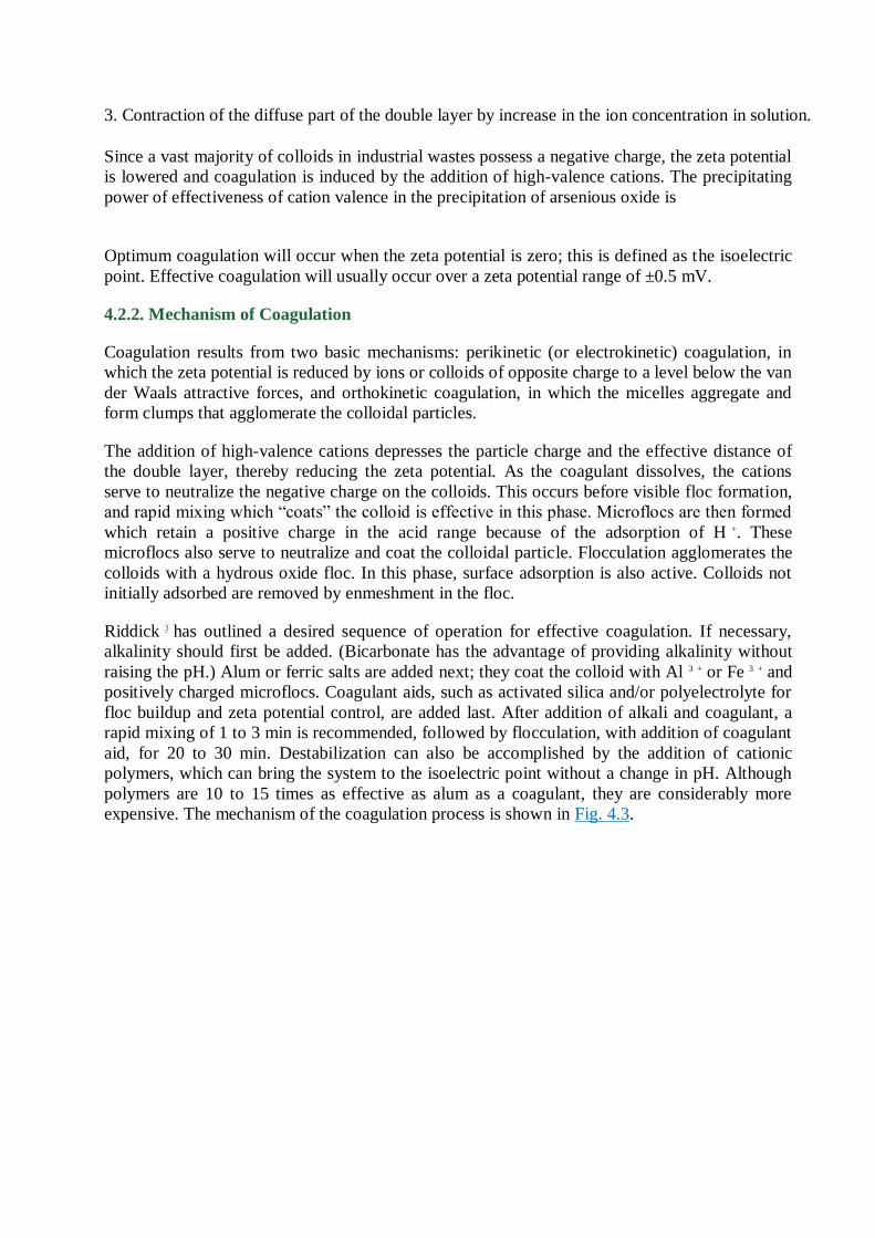
expensive. The mechanism of the coagulation process is shown in Fig. 4.3.

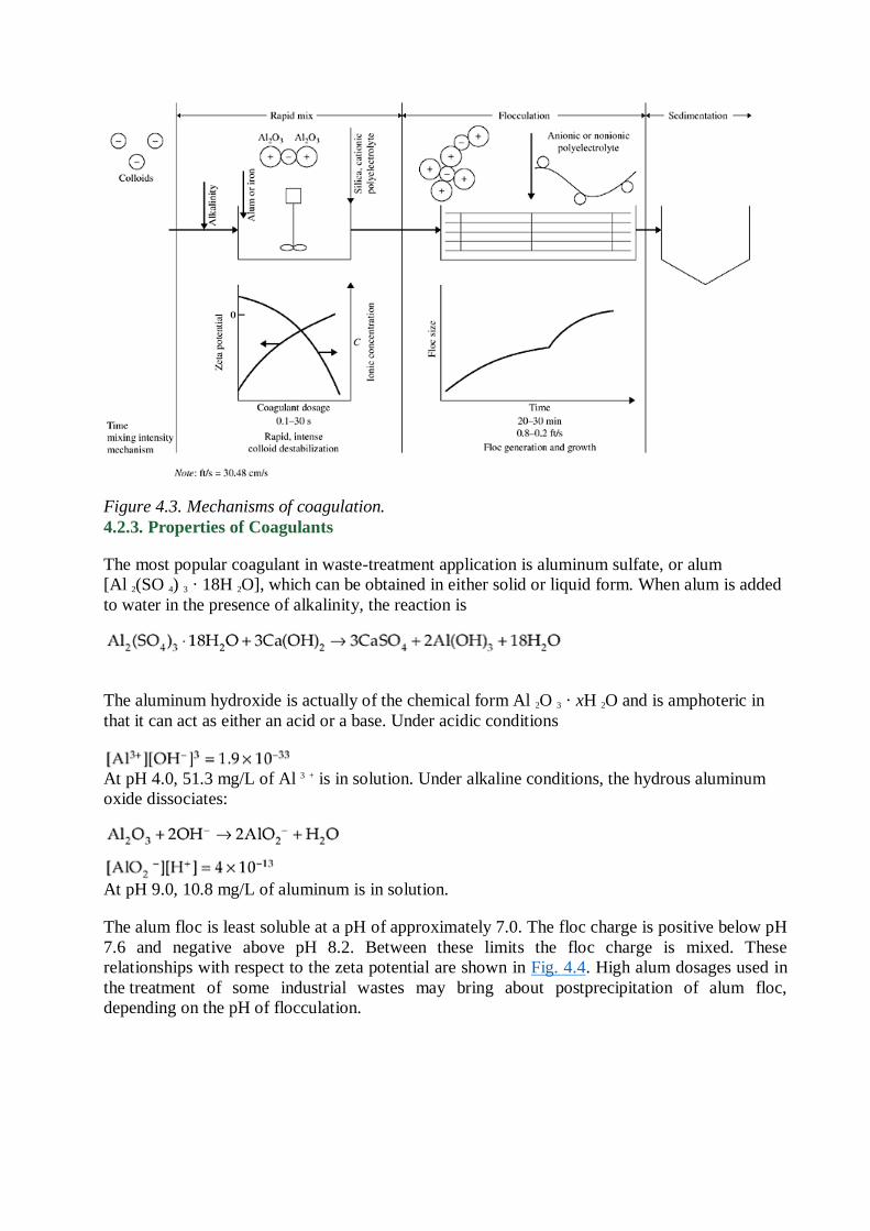
Figure 4.3. Mechanisms of coagulation.

4.2.3. Properties of Coagulants

The most popular coagulant in waste-treatment application is aluminum sulfate, or alum

[Al 2(SO 4) 3 · 18H 2O], which can be obtained in either solid or liquid form. When alum is added

to water in the presence of alkalinity, the reaction is

The aluminum hydroxide is actually of the chemical form Al 2O 3 · xH 2O and is amphoteric in

that it can act as either an acid or a base. Under acidic conditions

At pH 4.0, 51.3 mg/L of Al 3 + is in solution. Under alkaline conditions, the hydrous aluminum

oxide dissociates:

At pH 9.0, 10.8 mg/L of aluminum is in solution.

The alum floc is least soluble at a pH of approximately 7.0. The floc charge is positive below pH

7.6 and negative above pH 8.2. Between these limits the floc charge is mixed. These

relationships with respect to the zeta potential are shown in Fig. 4.4. High alum dosages used in

the treatment of some industrial wastes may bring about postprecipitation of alum floc,

depending on the pH of flocculation.

Figure 4.4. Zeta potential–pH plot for electrolytic aluminum hydroxide. (After Riddick, 1964.)

Ferric salts are also commonly used as coagulants but have the disadvantage of being corrosive

and more difficult to handle. An insoluble hydrous ferric oxide is produced over a pH range of

3.0 to 13.0:

The floc charge is positive in the acid range and negative in the alkaline range, with mixed

charges over the pH range 6.5 to 8.0.

The presence of anions will alter the range of effective flocculation. Sulfate ion will increase the

acid range but decrease the alkaline range. Chloride ion increases the range slightly on both

sides.

Lime is not a true coagulant but reacts with bicarbonate alkalinity to precipitate calcium

carbonate and with ortho-phosphate to precipitate calcium hydroxy apatite. Magnesium

hydroxide precipitates at high pH levels. Good clarification usually requires the presence of

some gelatinous Mg(OH) 2, but this makes the sludge more difficult to dewater. Lime sludge can

frequently be thickened, dewatered, and calcined to convert calcium carbonate to lime for reuse.

4.2.4. Coagulant Aids

The addition of some chemicals will enhance coagulation by promoting the growth of large,

rapid-settling flocs. Activated silica is a short-chain polymer that serves to bind together particles

of microfine aluminum hydrate and produces a tougher more durable floc. At high dosages,

silica will inhibit floc formation because of its electro-negative properties. The usual dosage is 5

to 10 mg/L and is usually used with alum.

Polyelectrolytes are high-molecular-weight polymers which contain adsorbable groups and form

bridges between particles or charged flocs. Large flocs (0.3 to 1 mm) are thus created when

small dosages of polyelectrolyte (1 to 5 mg/L) are added in conjunction with alum or ferric

chloride. The polyelectrolyte is substantially unaffected by pH and can serve as a coagulant itself

by reducing the effective charge on a colloid. There are three types of polyelectrolytes: a

cationic, which adsorbs on a negative colloid or floc particle; an anionic, which replaces the

anionic groups on a colloidal particle and permits hydrogen bonding between the colloid and the

polymer; and a nonionic, which adsorbs and flocculates by hydrogen bonding between the solid

surfaces and the polar groups in the polymer. Polymers do not add a significant amount of

dissolved ions and result in a reduced sludge volume and, often, enhanced dewaterability. The

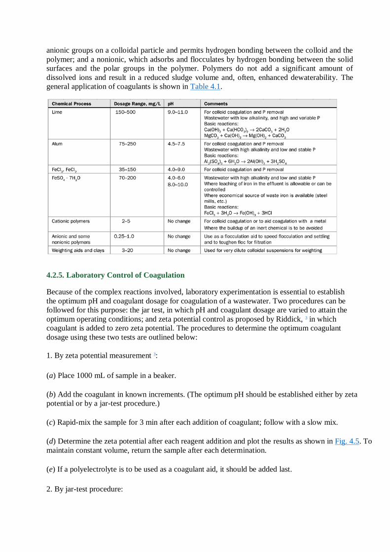
general application of coagulants is shown in Table 4.1.

4.2.5. Laboratory Control of Coagulation

Because of the complex reactions involved, laboratory experimentation is essential to establish

the optimum pH and coagulant dosage for coagulation of a wastewater. Two procedures can be

followed for this purpose: the jar test, in which pH and coagulant dosage are varied to attain the

optimum operating conditions; and zeta potential control as proposed by Riddick, 3 in which

coagulant is added to zero zeta potential. The procedures to determine the optimum coagulant

dosage using these two tests are outlined below:

1. By zeta potential measurement 3:

(a) Place 1000 mL of sample in a beaker.

(b) Add the coagulant in known increments. (The optimum pH should be established either by zeta

potential or by a jar-test procedure.)

(c) Rapid-mix the sample for 3 min after each addition of coagulant; follow with a slow mix.

(d) Determine the zeta potential after each reagent addition and plot the results as shown in Fig. 4.5. To

maintain constant volume, return the sample after each determination.

(e) If a polyelectrolyte is to be used as a coagulant aid, it should be added last.

2. By jar-test procedure:

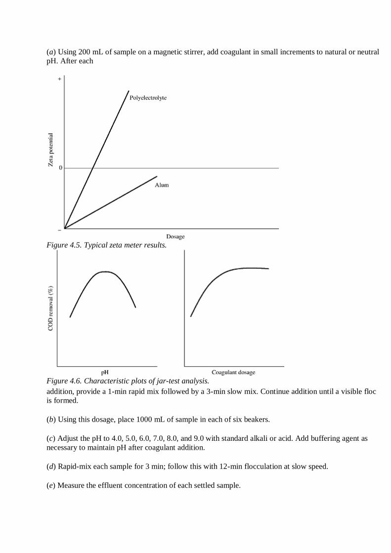
(a) Using 200 mL of sample on a magnetic stirrer, add coagulant in small increments to natural or neutral

pH. After each

Figure 4.5. Typical zeta meter results.

Figure 4.6. Characteristic plots of jar-test analysis.

addition, provide a 1-min rapid mix followed by a 3-min slow mix. Continue addition until a visible floc

is formed.

(b) Using this dosage, place 1000 mL of sample in each of six beakers.

(c) Adjust the pH to 4.0, 5.0, 6.0, 7.0, 8.0, and 9.0 with standard alkali or acid. Add buffering agent as

necessary to maintain pH after coagulant addition.

(d) Rapid-mix each sample for 3 min; follow this with 12-min flocculation at slow speed.

(e) Measure the effluent concentration of each settled sample.

(f) Plot the percent removal of characteristic versus pH and select the optimum pH (Fig. 4.6).

(g) Using this pH, repeat steps (b), (d), and (e), varying the coagulant dosage.

(h) Plot the percent removal versus the coagulant dosage and select the optimum dosage (Fig. 4.6).

(i) If a polyelectrolyte is used, repeat the procedure, adding polyelectrolyte toward the end of a rapid mix.

4.2.6. Coagulation Equipment

There are two basic types of equipment adaptable to the flocculation and coagulation of

industrial wastes. The conventional system uses a rapid-mix tank, followed by a flocculation

tank containing longitudinal paddles which provide slow mixing. The flocculated mixture is then

settled in conventional settling tanks.

A sludge-blanket unit combines mixing, flocculation, and settling in a single unit. Although

colloidal destabilization might be less effective than in the conventional system, there are distinct

advantages in recycling preformed floc. With lime and a few other coagulants, the time required

to form a settleable floc is a function of the time necessary for calcium carbonate or other

calcium precipitates to form nuclei on which other calcium materials can deposit and grow large

enough to settle. It is possible to reduce both coagulant dosage and the time of floc formation by

seeding the influent wastewater with previously formed nuclei or by recycling a portion of the

precipitated sludge. Recycling preformed floc can frequently reduce chemical dosages, the

blanket serves as a filter for improved effluent clarity, and denser sludges are frequently

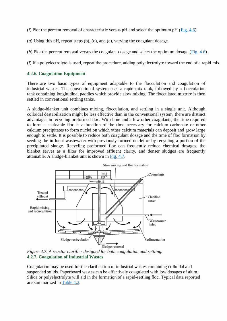
attainable. A sludge-blanket unit is shown in Fig. 4.7.

Figure 4.7. A reactor clarifier designed for both coagulation and settling.

4.2.7. Coagulation of Industrial Wastes

Coagulation may be used for the clarification of industrial wastes containing colloidal and

suspended solids. Paperboard wastes can be effectively coagulated with low dosages of alum.

Silica or polyelectrolyte will aid in the formation of a rapid-settling floc. Typical data reported

are summarized in Table 4.2.

Wastes containing emulsified oils can be clarified by coagulation. 7 An emulsion can consist of

droplets of oil in water. The oil droplets are of approximately 10 − 5 cm and are stabilized by

adsorbed ions. Emulsifying agents include soaps and anion-active agents. The emulsion can be

broken by ―salting out‖ with the addition of salts, such as CaCl 2. Flocculation will then effect

charge neutralization and entrainment, resulting in clarification. An emulsion can also frequently

be broken by lowering of the pH of the waste solution. An example of such a waste is that

produced by ball-bearing manufacture, which contains cleaning soaps and detergents, water-

soluble grinding oils, cutting oils, and phosphoric acid cleaners and solvents. Treatment of this

waste has been effected by the use of 800 mg/L alum, 450 mg/L H 2SO 4, and 45 mg/L

polyelectrolyte. The results obtained are summarized in Table 4.3a.

*Gluc. †15,000 gal/ton waste paper.

Note: gal/(d · ft 2) = 4.075 × 10 −2 m 3/(d · m 2)

gal/ton = 4.17 × 10 −3 m 3/t

The presence of anionic surface agents in a waste will increase the coagulant dosage. The polar

head of the surfactant molecule enters the double layer and stabilizes the negative colloids.

Industrial laundry wastes have been treated with H 2SO 4 followed by lime and alum; this has

resulted in a reduction of COD of 12,000 to 1800 mg/L and a reduction of suspended solids of

1620 to 105 mg/L. Chemical dosages of 1400 mg/L H 2SO 4, 1500 mg/L lime, and 300 mg/L

alum were required, yielding 25 percent by volume of settled sludge.

(a) Ball Bearing Manufacture*

Analysis

Influent Effluent

pH 10.3 7.1

Suspended solids, mg/L 544 40

Oil and grease, mg/L 302 28

Fe, mg/L 17.9 1.6

PO 4, mg/L 222 8.5

(b) Laundromat

Influent, mg/L Effluent, mg/L

ABS 63 0.1

BOD 243 90

COD 512 171

PO 4 267 150

CaCl 2 480

Cationic surfactant 88

pH 7.1 7.7

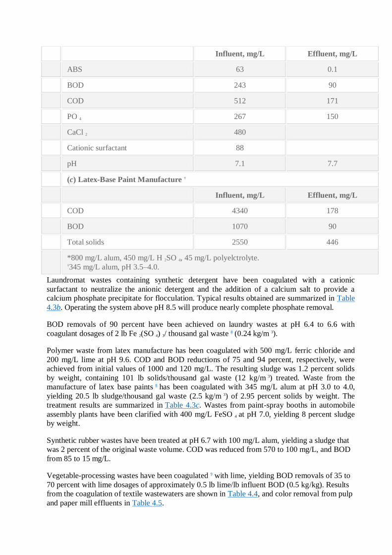
(c) Latex-Base Paint Manufacture †

Influent, mg/L Effluent, mg/L

COD 4340 178

BOD 1070 90

Total solids 2550 446

*800 mg/L alum, 450 mg/L H 2SO 4, 45 mg/L polyelctrolyte. †345 mg/L alum, pH 3.5–4.0.

Laundromat wastes containing synthetic detergent have been coagulated with a cationic

surfactant to neutralize the anionic detergent and the addition of a calcium salt to provide a

calcium phosphate precipitate for flocculation. Typical results obtained are summarized in Table

4.3b. Operating the system above pH 8.5 will produce nearly complete phosphate removal.

BOD removals of 90 percent have been achieved on laundry wastes at pH 6.4 to 6.6 with

coagulant dosages of 2 lb Fe 2(SO 4) 3/ thousand gal waste 8 (0.24 kg/m 3).

Polymer waste from latex manufacture has been coagulated with 500 mg/L ferric chloride and

200 mg/L lime at pH 9.6. COD and BOD reductions of 75 and 94 percent, respectively, were

achieved from initial values of 1000 and 120 mg/L. The resulting sludge was 1.2 percent solids

by weight, containing 101 lb solids/thousand gal waste (12 kg/m 3) treated. Waste from the

manufacture of latex base paints 8 has been coagulated with 345 mg/L alum at pH 3.0 to 4.0,

yielding 20.5 lb sludge/thousand gal waste (2.5 kg/m 3) of 2.95 percent solids by weight. The

treatment results are summarized in Table 4.3c. Wastes from paint-spray booths in automobile

assembly plants have been clarified with 400 mg/L FeSO 4 at pH 7.0, yielding 8 percent sludge

by weight.

Synthetic rubber wastes have been treated at pH 6.7 with 100 mg/L alum, yielding a sludge that

was 2 percent of the original waste volume. COD was reduced from 570 to 100 mg/L, and BOD

from 85 to 15 mg/L.

Vegetable-processing wastes have been coagulated 9 with lime, yielding BOD removals of 35 to

70 percent with lime dosages of approximately 0.5 lb lime/lb influent BOD (0.5 kg/kg). Results

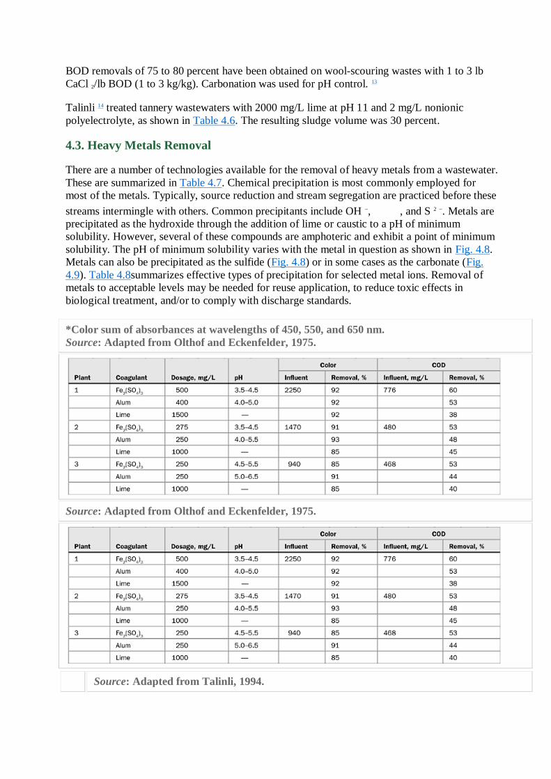
from the coagulation of textile wastewaters are shown in Table 4.4, and color removal from pulp

and paper mill effluents in Table 4.5.

BOD removals of 75 to 80 percent have been obtained on wool-scouring wastes with 1 to 3 lb

CaCl 2/lb BOD (1 to 3 kg/kg). Carbonation was used for pH control. 13

Talinli 14 treated tannery wastewaters with 2000 mg/L lime at pH 11 and 2 mg/L nonionic

polyelectrolyte, as shown in Table 4.6. The resulting sludge volume was 30 percent.

4.3. Heavy Metals Removal

There are a number of technologies available for the removal of heavy metals from a wastewater.

These are summarized in Table 4.7. Chemical precipitation is most commonly employed for

most of the metals. Typically, source reduction and stream segregation are practiced before these

streams intermingle with others. Common precipitants include OH −, , and S 2 −. Metals are

precipitated as the hydroxide through the addition of lime or caustic to a pH of minimum

solubility. However, several of these compounds are amphoteric and exhibit a point of minimum

solubility. The pH of minimum solubility varies with the metal in question as shown in Fig. 4.8.

Metals can also be precipitated as the sulfide (Fig. 4.8) or in some cases as the carbonate (Fig.

4.9). Table 4.8summarizes effective types of precipitation for selected metal ions. Removal of

metals to acceptable levels may be needed for reuse application, to reduce toxic effects in

biological treatment, and/or to comply with discharge standards.

*Color sum of absorbances at wavelengths of 450, 550, and 650 nm.

Source: Adapted from Olthof and Eckenfelder, 1975.

Source: Adapted from Olthof and Eckenfelder, 1975.

Source: Adapted from Talinli, 1994.

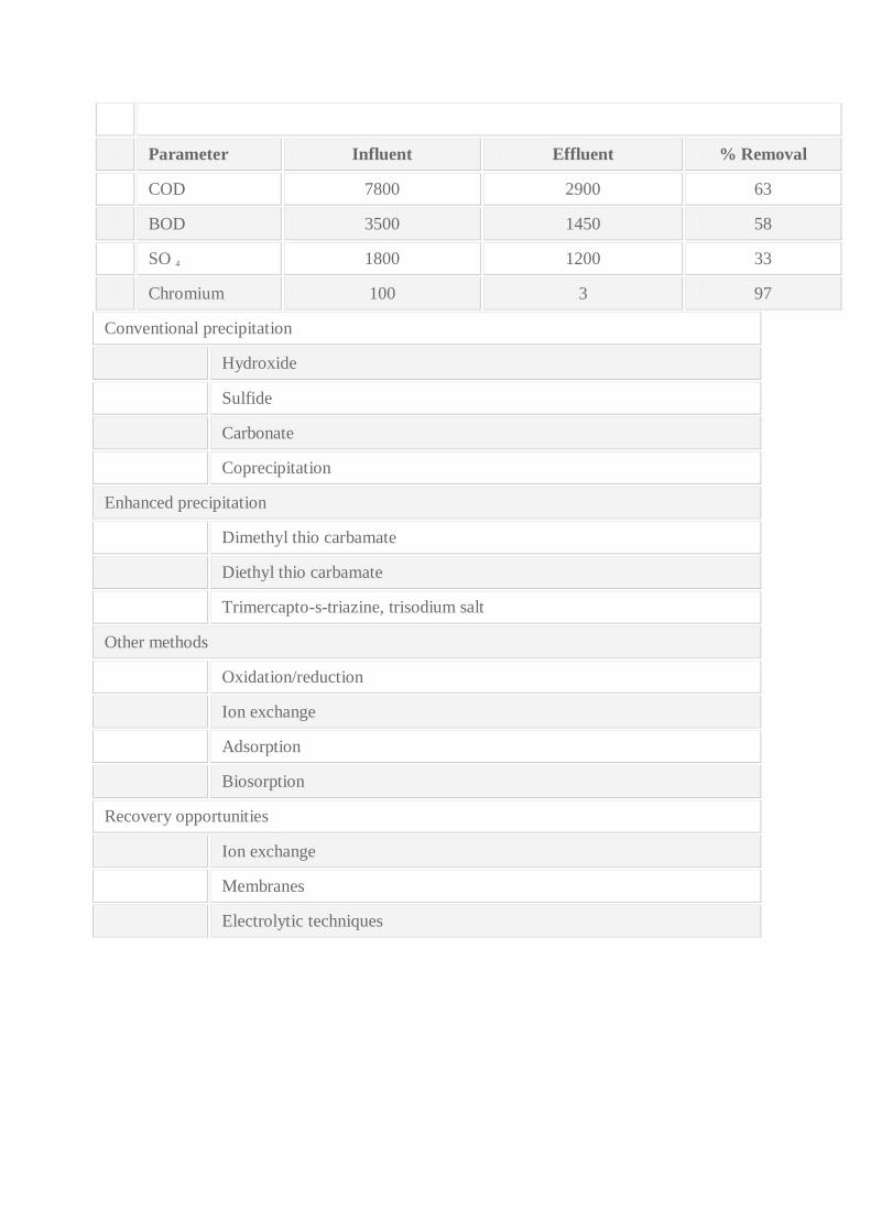
Parameter Influent Effluent % Removal

COD 7800 2900 63

BOD 3500 1450 58

SO 4 1800 1200 33

Chromium 100 3 97

Conventional precipitation

Hydroxide

Sulfide

Carbonate

Coprecipitation

Enhanced precipitation

Dimethyl thio carbamate

Diethyl thio carbamate

Trimercapto-s-triazine, trisodium salt

Other methods

Oxidation/reduction

Ion exchange

Adsorption

Biosorption

Recovery opportunities

Ion exchange

Membranes

Electrolytic techniques

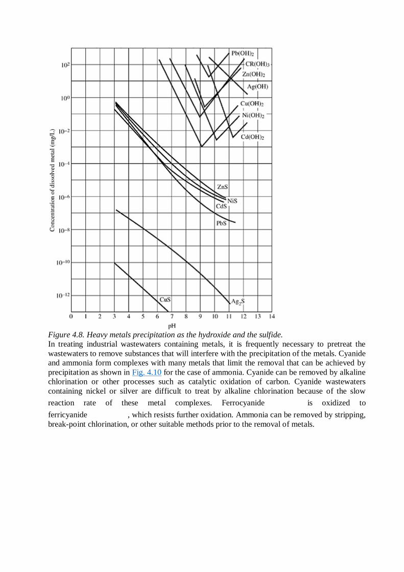
Figure 4.8. Heavy metals precipitation as the hydroxide and the sulfide.

In treating industrial wastewaters containing metals, it is frequently necessary to pretreat the

wastewaters to remove substances that will interfere with the precipitation of the metals. Cyanide

and ammonia form complexes with many metals that limit the removal that can be achieved by

precipitation as shown in Fig. 4.10 for the case of ammonia. Cyanide can be removed by alkaline

chlorination or other processes such as catalytic oxidation of carbon. Cyanide wastewaters

containing nickel or silver are difficult to treat by alkaline chlorination because of the slow

reaction rate of these metal complexes. Ferrocyanide is oxidized to

ferricyanide , which resists further oxidation. Ammonia can be removed by stripping,

break-point chlorination, or other suitable methods prior to the removal of metals.

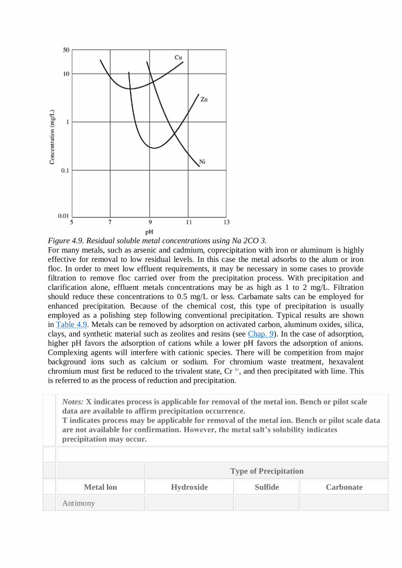
Figure 4.9. Residual soluble metal concentrations using Na 2CO 3.

For many metals, such as arsenic and cadmium, coprecipitation with iron or aluminum is highly

effective for removal to low residual levels. In this case the metal adsorbs to the alum or iron

floc. In order to meet low effluent requirements, it may be necessary in some cases to provide

filtration to remove floc carried over from the precipitation process. With precipitation and

clarification alone, effluent metals concentrations may be as high as 1 to 2 mg/L. Filtration

should reduce these concentrations to 0.5 mg/L or less. Carbamate salts can be employed for

enhanced precipitation. Because of the chemical cost, this type of precipitation is usually

employed as a polishing step following conventional precipitation. Typical results are shown

in Table 4.9. Metals can be removed by adsorption on activated carbon, aluminum oxides, silica,

clays, and synthetic material such as zeolites and resins (see Chap. 9). In the case of adsorption,

higher pH favors the adsorption of cations while a lower pH favors the adsorption of anions.

Complexing agents will interfere with cationic species. There will be competition from major

background ions such as calcium or sodium. For chromium waste treatment, hexavalent

chromium must first be reduced to the trivalent state, Cr 3+, and then precipitated with lime. This

is referred to as the process of reduction and precipitation.

Notes: X indicates process is applicable for removal of the metal ion. Bench or pilot scale

data are available to affirm precipitation occurrence.

T indicates process may be applicable for removal of the metal ion. Bench or pilot scale data

are not available for confirmation. However, the metal salt’s solubility indicates

precipitation may occur.

Type of Precipitation

Metal lon Hydroxide Sulfide Carbonate

Antimony

Arsenic X X

Beryllium X T

Cadmium X X

Chromium X X

Copper X X

Lead X X X

Mercury X

Nickel X X X

Selenium

Silver X T

Thallium T

Zinc X X T

Iron X X

Manganese X T

4.3.1. Arsenic

Arsenic and arsenical compounds are present in wastewaters from the metallurgical industry,

glassware and ceramic production, tannery operation, dyestuff manufacture, pesticide

manufacture, some organic and inorganic chemicals manufacture, petroleum refining, and the

rare-earth industry. Arsenic is removed from wastewater by chemical precipitation. Enhanced

performance is achieved as arsenate ( , As 5 +) rather than arsenite ( , As 3+).

Arsenite is therefore usually oxidized to arsenate prior to precipitation. Effluent arsenic levels of

0.05 mg/L are obtainable by precipitation of the arsenic as the sulfide by the addition of sodium

or hydrogen sulfide at pH of 6 to 7. In order to meet reported effluent levels, polishing of the

effluent by filtration is usually required.

Arsenic present in low concentrations can also be reduced by filtration through activated carbon.

Effluent concentrations of 0.06 mg/L arsenic have been reported from an initial concentration of

0.2 mg/L. Arsenic is removed by coprecipitation with a ferric hydroxide floc that ties up the

arsenic and removes it from solution. Effluent concentrations of less than 0.005 mg/L have been

reported from this process.

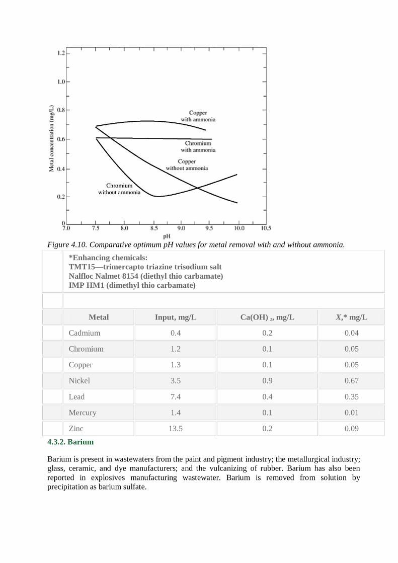
Figure 4.10. Comparative optimum pH values for metal removal with and without ammonia.

*Enhancing chemicals:

TMT15—trimercapto triazine trisodium salt

Nalfloc Nalmet 8154 (diethyl thio carbamate)

IMP HM1 (dimethyl thio carbamate)

Metal Input, mg/L Ca(OH) 2, mg/L X,* mg/L

Cadmium 0.4 0.2 0.04

Chromium 1.2 0.1 0.05

Copper 1.3 0.1 0.05

Nickel 3.5 0.9 0.67

Lead 7.4 0.4 0.35

Mercury 1.4 0.1 0.01

Zinc 13.5 0.2 0.09

4.3.2. Barium

Barium is present in wastewaters from the paint and pigment industry; the metallurgical industry;

glass, ceramic, and dye manufacturers; and the vulcanizing of rubber. Barium has also been

reported in explosives manufacturing wastewater. Barium is removed from solution by

precipitation as barium sulfate.

Barium sulfate is extremely insoluble, having a maximum theoretical solubility at 25ºC of

approximately 1.4 mg/L as barium at stoichiometric concentrations of barium and sulfate. The

solubility level of barium can be reduced in the presence of excess sulfate. Coagulation of

barium salts as the sulfate is capable of reducing barium to effluent levels of 0.03 to 0.3 mg/L.

Barium can also be removed from solution by ion exchange and electrodialysis, although these

processes are more expensive than chemical precipitation.

4.3.3. Cadmium

Cadmium is present in wastewaters from metallurgical alloying, ceramics, electroplating,

photography, pigment works, textile printing, chemical industries, and lead mine drainage.

Cadmium is removed from wastewaters by precipitation or ion exchange. In some cases,

electrolytic and evaporative recovery processes can be employed, provided the wastewater is in a

concentrated form. Cadmium forms an insoluble and highly stable hydroxide at an alkaline pH.

Cadmium in solution is approximately 1 mg/L at pH 8 and 0.05 mg/L at pH 10 to 11.

Coprecipitation with iron hydroxide at pH 6.5 will reduce cadmium to 0.008 mg/L; iron

hydroxide at pH 8.5 reduces cadmium to 0.05 mg/L. Sulfide and lime precipitation with filtration

will yield 0.002 to 0.03 mg/L at pH 8.5 to 10. Cadmium is not precipitated in the presence of

complexing ions, such as cyanide. In these cases, it is necessary to pretreat the wastewater to

destroy the complexing agent. In the case of cyanide, cyanide destruction is necessary prior to

cadmium precipitation. A hydrogen peroxide oxidation precipitation system has been developed

that simultaneously oxidizes cyanides and forms the oxide of cadmium, thereby yielding

cadmium, whose recovery is feasible. Results for the hydroxide precipitation of cadmium are

shown in Table 4.10.

4.3.4. Chromium

The reducing agents commonly used for chromium wastes are ferrous sulfate, sodium meta-

bisulfite, or sulfur dioxide. Ferrous sulfate and sodium meta-bisulfite may be dry- or solution-

fed; SO 2 is diffused into the system directly from gas cylinders. Since the reduction of

chromium is most effective at acidic pH values, a reducing agent with acidic properties is

desirable. When ferrous sulfate is used as the reducing agent, the Fe 2+ is oxidized to Fe3+; if

meta-bisulfite or sulfur dioxide is used, the negative radical is converted to . The

general reactions are

Method Treatment

pH

Initial Cd,

mg/L

Final Cd,

mg/L

Hydroxide precipitation 8.0 — 1.0

9.0 — 0.54

10.0 — 0.10

9.3–10.6 4.0 0.20

Hydroxide precipitation plus filtration 10.0 0.34 0.054

10.0 0.34 0.033

Hydroxide precipitation plus filtration 11.0 — 0.00075

11.0 — 0.00070

Hydroxide precipitation plus filtration 11.5 — 0.014

Hydroxide precipitation plus filtration — — 0.08

Coprecipitation with ferrous

hydroxide

6.0 — 0.050

Coprecipitation with ferrous

hydroxide

10.0 — 0.044

Coprecipitation with alum 6.4 0.7 0.39

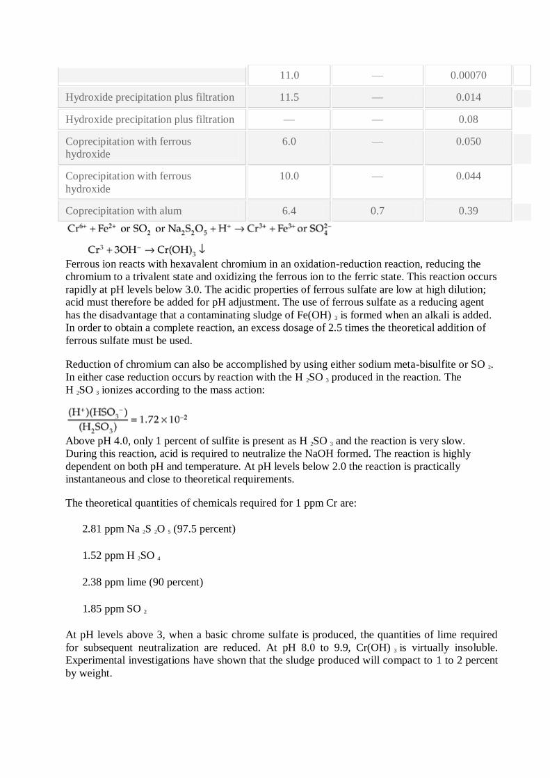
Ferrous ion reacts with hexavalent chromium in an oxidation-reduction reaction, reducing the

chromium to a trivalent state and oxidizing the ferrous ion to the ferric state. This reaction occurs

rapidly at pH levels below 3.0. The acidic properties of ferrous sulfate are low at high dilution;

acid must therefore be added for pH adjustment. The use of ferrous sulfate as a reducing agent

has the disadvantage that a contaminating sludge of Fe(OH) 3 is formed when an alkali is added.

In order to obtain a complete reaction, an excess dosage of 2.5 times the theoretical addition of

ferrous sulfate must be used.

Reduction of chromium can also be accomplished by using either sodium meta-bisulfite or SO 2.

In either case reduction occurs by reaction with the H 2SO 3 produced in the reaction. The

H 2SO 3 ionizes according to the mass action:

Above pH 4.0, only 1 percent of sulfite is present as H 2SO 3 and the reaction is very slow.

During this reaction, acid is required to neutralize the NaOH formed. The reaction is highly

dependent on both pH and temperature. At pH levels below 2.0 the reaction is practically

instantaneous and close to theoretical requirements.

The theoretical quantities of chemicals required for 1 ppm Cr are:

2.81 ppm Na 2S 2O 5 (97.5 percent)

1.52 ppm H 2SO 4

2.38 ppm lime (90 percent)

1.85 ppm SO 2

At pH levels above 3, when a basic chrome sulfate is produced, the quantities of lime required

for subsequent neutralization are reduced. At pH 8.0 to 9.9, Cr(OH) 3 is virtually insoluble.

Experimental investigations have shown that the sludge produced will compact to 1 to 2 percent

by weight.

Since dissolved oxygen is usually present in wastewaters, an excess of SO 2 must be added to

account for the oxidation of the to :

An excess dosage of 35 ppm SO 2 will usually be sufficient for reaction with the dissolved

oxygen present.

The acid requirements for the reduction of Cr 6+ depend on the acidity of the original waste, the

pH of the reduction reaction, and the type of reducing agent used (e.g., SO 2 produces an acid but

metabisulfite does not). Since it is difficult, if not impossible, to predict these requirements, it is

usually necessary to titrate a sample to the desired pH endpoint with standardized acid.

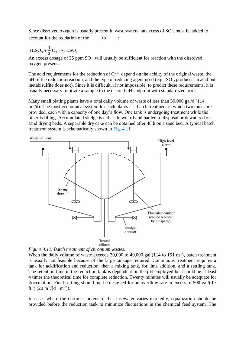
Many small plating plants have a total daily volume of waste of less than 30,000 gal/d (114

m 3/d). The most economical system for such plants is a batch treatment in which two tanks are

provided, each with a capacity of one day’s flow. One tank is undergoing treatment while the

other is filling. Accumulated sludge is either drawn off and hauled to disposal or dewatered on

sand drying beds. A separable dry cake can be obtained after 48 h on a sand bed. A typical batch

treatment system is schematically shown in Fig. 4.11.

Figure 4.11. Batch treatment of chromium wastes.

When the daily volume of waste exceeds 30,000 to 40,000 gal (114 to 151 m 3), batch treatment

is usually not feasible because of the large tankage required. Continuous treatment requires a

tank for acidification and reduction, then a mixing tank, for lime addition, and a settling tank.

The retention time in the reduction tank is dependent on the pH employed but should be at least

4 times the theoretical time for complete reduction. Twenty minutes will usually be adequate for

flocculation. Final settling should not be designed for an overflow rate in excess of 500 gal/(d ·

ft 2) (20 m 3/[d · m 2]).

In cases where the chrome content of the rinsewater varies markedly, equalization should be

provided before the reduction tank to minimize fluctuations in the chemical feed system. The

fluctuation in chrome content can be minimized by provision of a drain station before the rinse

tanks.

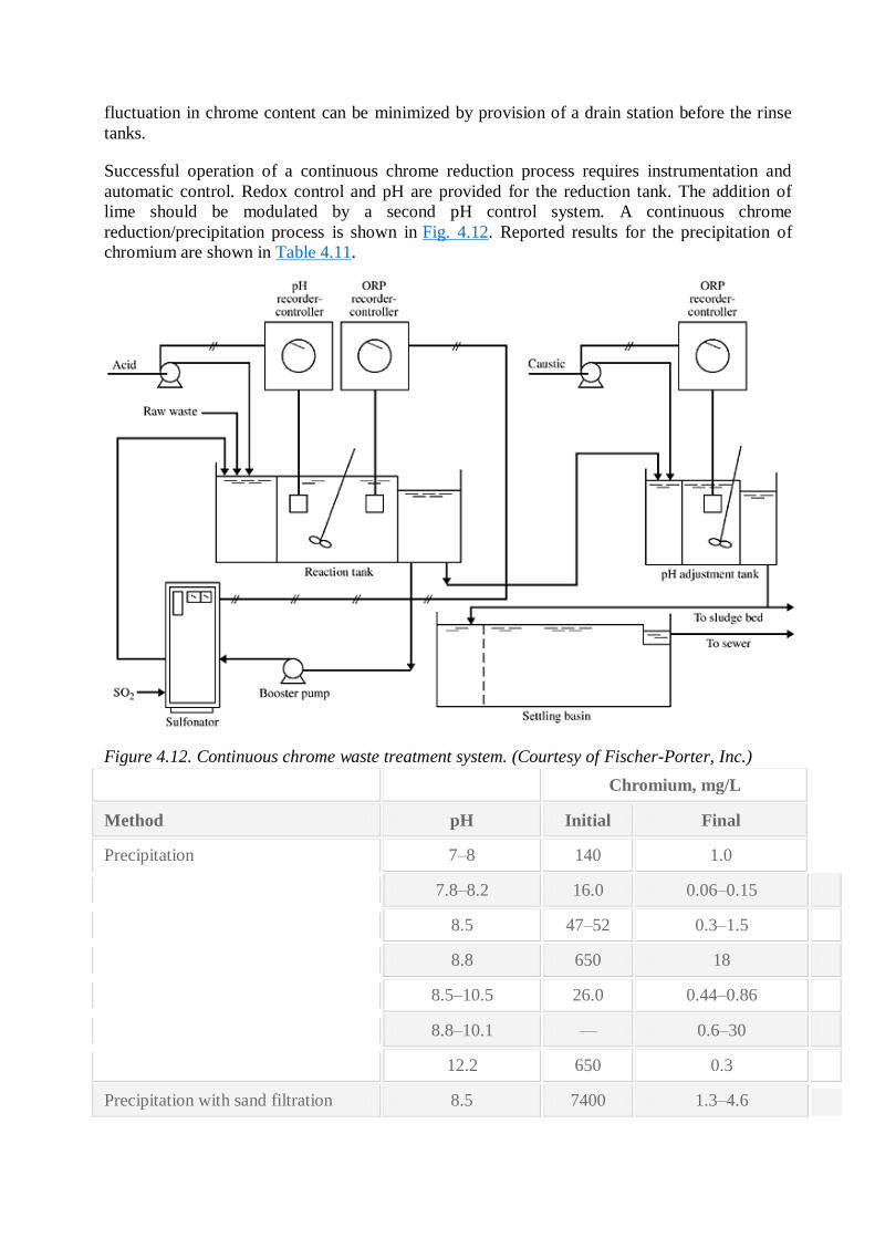
Successful operation of a continuous chrome reduction process requires instrumentation and

automatic control. Redox control and pH are provided for the reduction tank. The addition of

lime should be modulated by a second pH control system. A continuous chrome

reduction/precipitation process is shown in Fig. 4.12. Reported results for the precipitation of

chromium are shown in Table 4.11.

Figure 4.12. Continuous chrome waste treatment system. (Courtesy of Fischer-Porter, Inc.)

Chromium, mg/L

Method pH Initial Final

Precipitation 7–8 140 1.0

7.8–8.2 16.0 0.06–0.15

8.5 47–52 0.3–1.5

8.8 650 18

8.5–10.5 26.0 0.44–0.86

8.8–10.1 — 0.6–30

12.2 650 0.3

Precipitation with sand filtration 8.5 7400 1.3–4.6

8.5 7400 0.3–1.3

9.8–10.0 49.4 0.17

9.8–10.0 49.4 0.05

*lb chromate/ft 3 resin.

Source: Adapted from Patterson, 1985.

Chromium, mg/L

Wastewater Source Influent Effluent Resin Capacity*

Cooling tower blowdown 17.9 1.8 5–6

10.0 1.0 2.5–4.5

7.4–10.3 1.0 —

9.0 0.2 2.5

Plating rinsewater 44.8 0.025 1.7–2.0

41.6 0.01 5.2–6.3

Pigment manufacture 1210 <0.5 —

Removal of chromium by ion exchange is shown in Table 4.12. An example of metals removal is

shown inExample 4.2.

Example 4.2.

30,000 gal/d (114 m 3/d) of a waste containing 49 mg/L Cr 6 +, 11 mg/L Cu, and 12 mg/L Zn

is to be treated daily by using SO 2. Compute the chemical requirements and the daily sludge

production. (Assume the waste contains 5 mg/L O 2.)

Solution

(a) SO 2 requirements are as follows. For Cr 6+

and for O 2, where 1 part of O 2 requires 4 parts of SO 2:

(b) Lime requirements are as follows. For Cr 3 +:

and for Cu and Zn (each part of Cu and Zn requiring 1.3 parts of 90 percent lime for

precipitation):

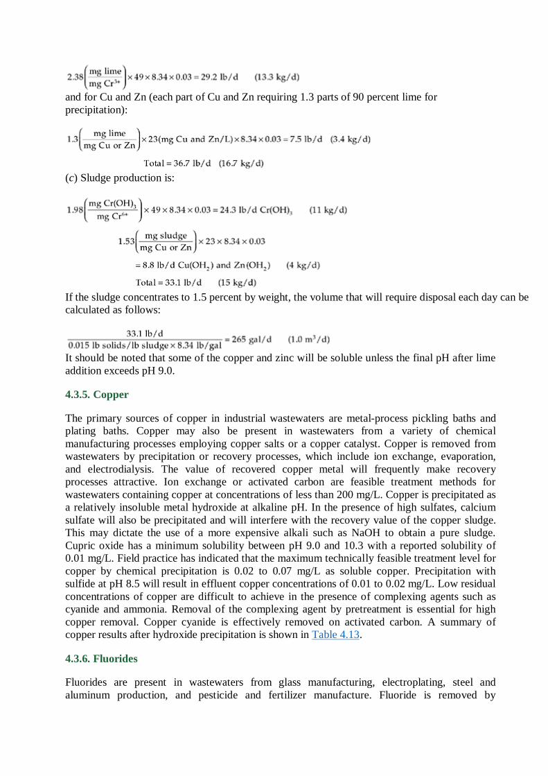
(c) Sludge production is:

If the sludge concentrates to 1.5 percent by weight, the volume that will require disposal each day can be

calculated as follows:

It should be noted that some of the copper and zinc will be soluble unless the final pH after lime

addition exceeds pH 9.0.

4.3.5. Copper

The primary sources of copper in industrial wastewaters are metal-process pickling baths and

plating baths. Copper may also be present in wastewaters from a variety of chemical

manufacturing processes employing copper salts or a copper catalyst. Copper is removed from

wastewaters by precipitation or recovery processes, which include ion exchange, evaporation,

and electrodialysis. The value of recovered copper metal will frequently make recovery

processes attractive. Ion exchange or activated carbon are feasible treatment methods for

wastewaters containing copper at concentrations of less than 200 mg/L. Copper is precipitated as

a relatively insoluble metal hydroxide at alkaline pH. In the presence of high sulfates, calcium

sulfate will also be precipitated and will interfere with the recovery value of the copper sludge.

This may dictate the use of a more expensive alkali such as NaOH to obtain a pure sludge.

Cupric oxide has a minimum solubility between pH 9.0 and 10.3 with a reported solubility of

0.01 mg/L. Field practice has indicated that the maximum technically feasible treatment level for

copper by chemical precipitation is 0.02 to 0.07 mg/L as soluble copper. Precipitation with

sulfide at pH 8.5 will result in effluent copper concentrations of 0.01 to 0.02 mg/L. Low residual

concentrations of copper are difficult to achieve in the presence of complexing agents such as

cyanide and ammonia. Removal of the complexing agent by pretreatment is essential for high

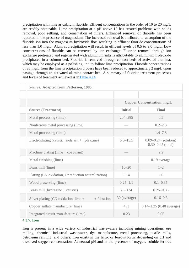
copper removal. Copper cyanide is effectively removed on activated carbon. A summary of

copper results after hydroxide precipitation is shown in Table 4.13.

4.3.6. Fluorides

Fluorides are present in wastewaters from glass manufacturing, electroplating, steel and

aluminum production, and pesticide and fertilizer manufacture. Fluoride is removed by

precipitation with lime as calcium fluoride. Effluent concentrations in the order of 10 to 20 mg/L

are readily obtainable. Lime precipitation at a pH above 12 has created problems with solids

removal, poor settling, and cementation of filters. Enhanced removal of fluoride has been

reported in the presence of magnesium. The increased removal is attributed to adsorption of the

fluoride ion into the magnesium hydroxide floc, resulting in effluent fluoride concentrations of

less than 1.0 mg/L. Alum coprecipitation will result in effluent levels of 0.5 to 2.0 mg/L. Low

concentrations of fluoride can be removed by ion exchange. Fluoride removal through ion

exchange pretreated and regenerated with aluminum salts is attributable to aluminum hydroxide

precipitated in a column bed. Fluoride is removed through contact beds of activated alumina,

which may be employed as a polishing unit to follow lime precipitation. Fluoride concentrations

of 30 mg/L from the lime precipitation process have been reduced to approximately 2 mg/L upon

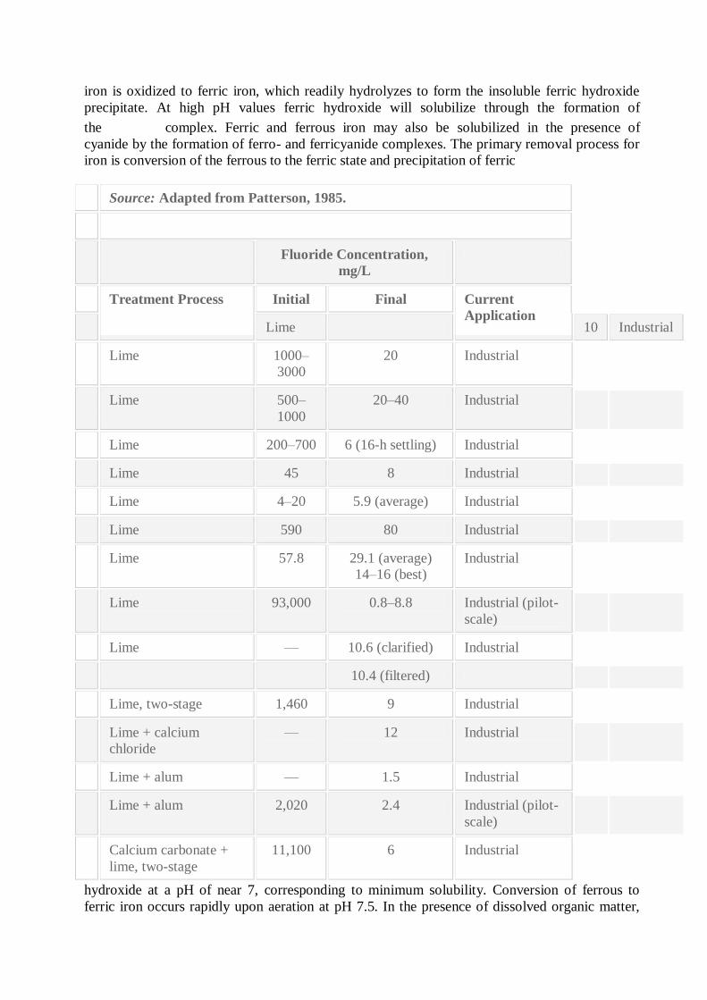
passage through an activated alumina contact bed. A summary of fluoride treatment processes

and levels of treatment achieved is inTable 4.14.

Source: Adapted from Patterson, 1985.

Copper Concentration, mg/L

Source (Treatment) Initial Final

Metal processing (lime) 204–385 0.5

Nonferrous metal processing (lime) — 0.2–2.3

Metal processing (lime) — 1.4–7.8

Electroplating (caustic, soda ash + hydrazine) 6.0–15.5 0.09–0.24 (solution)

0.30–0.45 (total)

Machine plating (lime + coagulant) — 2.2

Metal finishing (lime) — 0.19 average

Brass mill (lime) 10–20 1–2

Plating (CN oxidation, Cr reduction neutralization) 11.4 2.0

Wood preserving (lime) 0.25–1.1 0.1–0.35

Brass mill (hydrazine + caustic) 75–124 0.25–0.85

Silver plating (CN oxidation, lime + + filtration 30 (average) 0.16–0.3

Copper sulfate manufacture (lime) 433 0.14–1.25 (0.48 average)

Integrated circuit manufacture (lime) 0.23 0.05

4.3.7. Iron

Iron is present in a wide variety of industrial wastewaters including mining operations, ore

milling, chemical industrial wastewater, dye manufacture, metal processing, textile mills,

petroleum refining, and others. Iron exists in the ferric or ferrous form, depending on pH and

dissolved oxygen concentration. At neutral pH and in the presence of oxygen, soluble ferrous

iron is oxidized to ferric iron, which readily hydrolyzes to form the insoluble ferric hydroxide

precipitate. At high pH values ferric hydroxide will solubilize through the formation of

the complex. Ferric and ferrous iron may also be solubilized in the presence of

cyanide by the formation of ferro- and ferricyanide complexes. The primary removal process for

iron is conversion of the ferrous to the ferric state and precipitation of ferric

Source: Adapted from Patterson, 1985.

Fluoride Concentration,

mg/L

Treatment Process Initial Final Current

Application Lime 10 Industrial

Lime 1000–

3000

20 Industrial

Lime 500–

1000

20–40 Industrial

Lime 200–700 6 (16-h settling) Industrial

Lime 45 8 Industrial

Lime 4–20 5.9 (average) Industrial

Lime 590 80 Industrial

Lime 57.8 29.1 (average)

14–16 (best)

Industrial

Lime 93,000 0.8–8.8 Industrial (pilot-

scale)

Lime — 10.6 (clarified) Industrial

10.4 (filtered)

Lime, two-stage 1,460 9 Industrial

Lime + calcium

chloride

— 12 Industrial

Lime + alum — 1.5 Industrial

Lime + alum 2,020 2.4 Industrial (pilot-

scale)

Calcium carbonate +

lime, two-stage

11,100 6 Industrial

hydroxide at a pH of near 7, corresponding to minimum solubility. Conversion of ferrous to

ferric iron occurs rapidly upon aeration at pH 7.5. In the presence of dissolved organic matter,

the iron oxidation rate is reduced. Two-stage hydroxide precipitation or sulfate precipitation will

reduce iron to 0.01 mg/L.

4.3.8. Lead

Lead is present in wastewaters from storage-battery manufacture. Lead is generally removed

from wastewaters by precipitation as the carbonate, PbCO 3, or the hydroxide, Pb(OH) 2. Lead is

effectively precipitated as the carbonate by the addition of soda ash, resulting in effluent-

dissolved lead concentrations of 0.01 to 0.03 mg/L at a pH of 9.0 to 9.5. Precipitation with lime

at pH 11.5 resulted in effluent concentrations of 0.019 to 0.2 mg/L. Precipitation as the sulfide to

0.01 mg/L can be accomplished with sodium sulfide at a pH of 7.5 to 8.5.

4.3.9. Manganese

Manganese and its salts are found in wastewaters from manufacture of steel alloy, dry-cell

batteries, glass and ceramics, paint and varnish, and inks and dye. Among the many forms and

compounds of manganese only the manganous salts and the highly oxidized permanganate anion

are appreciably soluble. The latter is a strong oxidant that is reduced under normal circumstances

to insoluble manganese dioxide. Treatment technology for the removal of manganese involves

conversion of the soluble manganous ion to an insoluble precipitate. Removal is effected by

oxidation of the manganous ion and separation of the resulting insoluble oxides and hydroxides.

Manganous ion has a low reactivity with oxygen and simple aeration is not an effective

technique below pH 9. It has been reported that even at high pH levels, organic matter in solution

can combine with manganese and prevent its oxidation by simple aeration. A reaction pH above

9.4 is required to achieve significant manganese reduction by precipitation. The use of chemical

oxidants to convert manganous ion to insoluble manganese dioxide in conjunction with

coagulation and filtration has been employed. The presence of copper ion enhances air oxidation

of manganese, and chlorine dioxide rapidly oxidizes manganese to the insoluble form.

Permanganate has successfully been employed in the oxidation of manganese. Ozone has been

employed in conjunction with lime for the oxidation and removal of manganese. The drawback

in the application of ion exchange is the nonselective removal of other ions, which increases

operating costs.

4.3.10. Mercury

The major consumptive user of mercury in the United States is the chloralkali industry. Mercury

is also used in the electrical and electronics industry, explosives manufacturing, the photographic

industry, and the pesticide and preservative industry. Mercury is used as a catalyst in the

chemical and petrochemical industry. Mercury is also found in most laboratory wastewaters.

Power generation is a large source of mercury release into the environment through the

combustion of fossil fuel. When scrubber devices are installed on thermal power plant stacks for

sulfur dioxide removal, accumulation of mercury is possible if extensive recycle is practiced.

Mercury can be removed from wastewaters by precipitation, ion exchange, and adsorption.

Mercury ions can be reduced upon contact with other metals such as copper, zinc, or aluminum.

In most cases mercury recovery can be achieved by distillation. For precipitation, mercury

compounds must be oxidized to the mercuric ion. Table 4.15 shows effluent levels achievable by

candidate technology.

Technology Effluent, μg/L

Sulfide precipitation 10–20

Alum coprecipitation 1–10

Iron coprecipitation 0.5–5

Ion exchange 1–5

Carbon adsorption

Influent —

High 20

Moderate 2

Low 0.25

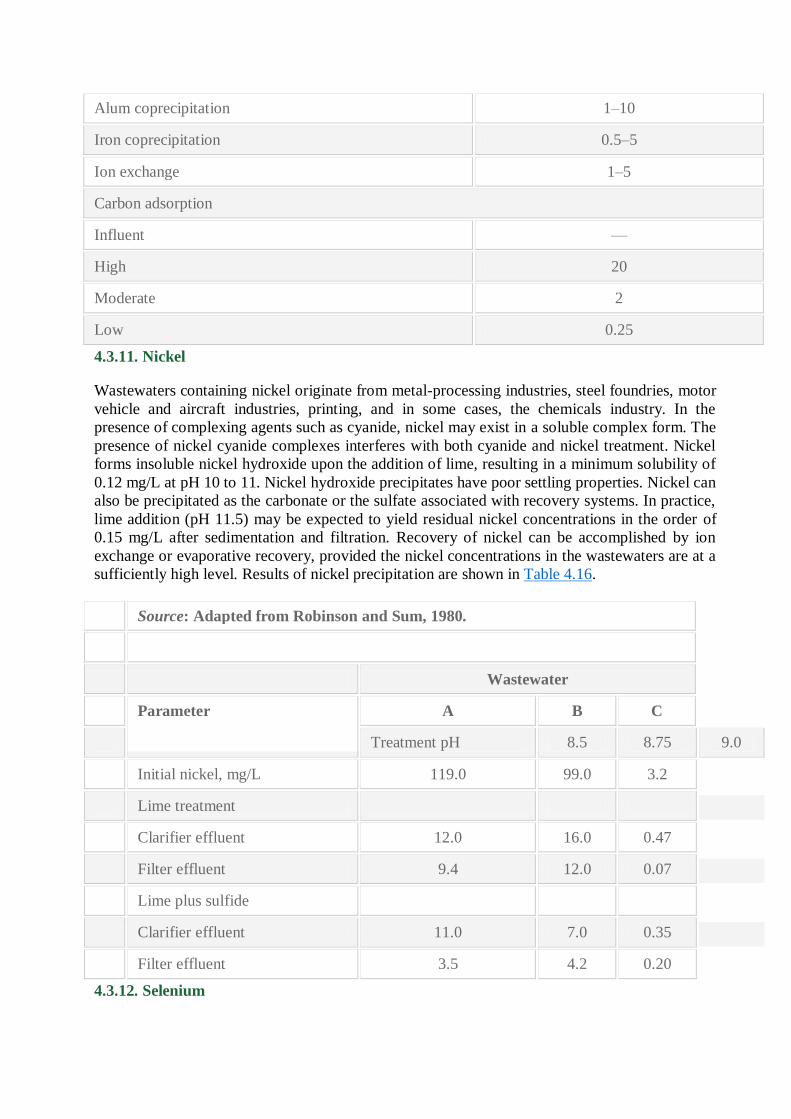
4.3.11. Nickel

Wastewaters containing nickel originate from metal-processing industries, steel foundries, motor

vehicle and aircraft industries, printing, and in some cases, the chemicals industry. In the

presence of complexing agents such as cyanide, nickel may exist in a soluble complex form. The

presence of nickel cyanide complexes interferes with both cyanide and nickel treatment. Nickel

forms insoluble nickel hydroxide upon the addition of lime, resulting in a minimum solubility of

0.12 mg/L at pH 10 to 11. Nickel hydroxide precipitates have poor settling properties. Nickel can

also be precipitated as the carbonate or the sulfate associated with recovery systems. In practice,

lime addition (pH 11.5) may be expected to yield residual nickel concentrations in the order of

0.15 mg/L after sedimentation and filtration. Recovery of nickel can be accomplished by ion

exchange or evaporative recovery, provided the nickel concentrations in the wastewaters are at a

sufficiently high level. Results of nickel precipitation are shown in Table 4.16.

Source: Adapted from Robinson and Sum, 1980.

Wastewater

Parameter A B C

Treatment pH 8.5 8.75 9.0

Initial nickel, mg/L 119.0 99.0 3.2

Lime treatment

Clarifier effluent 12.0 16.0 0.47

Filter effluent 9.4 12.0 0.07

Lime plus sulfide

Clarifier effluent 11.0 7.0 0.35

Filter effluent 3.5 4.2 0.20

4.3.12. Selenium

Selenium may be present in various types of paper, fly ash, and metallic sulfide ores. The

selenious ion appears to be the most common form of selenium in wastewater, except for

pigment and dye wastes, which contain selenide (yellow cadmium selenide). Selenium can be

removed from wastewaters by precipitation as the sulfide at a pH of 6.6. Effluent levels of 0.05

mg/L are reported. Ferric hydroxide coprecipitation at pH 6.2 will reduce selenium to a range of

0.01 to 0.05 mg/L. Alumina adsorption results in effluent levels of 0.005 to 0.02 mg/L.

4.3.13. Silver

Soluble silver, usually in the form of silver nitrate, is found in wastewaters from the porcelain,

photographic, electroplating, and ink manufacturing industries. Treatment technology for the

removal of silver usually considers recovery because of the high value of the metal. Basic

treatment methods include precipitation, ion exchange, reductive exchange, and electrolytic

recovery. Silver is removed from wastewater by precipitation as silver chloride, which is an

extremely insoluble precipitate resulting in the maximum silver concentration at 25ºC of

approximately 1.4 mg/L. An excess of chloride will reduce this value, but greater excess

concentrations will increase the solubility of silver through the formation of soluble silver

chloride complexes. Silver can be selectivelyprecipitated as silver chloride from a mixed-metal

wastestream without initial wastewater segregation or concurrent precipitation of other metals. If

the treatment conditions are alkaline, resulting in precipitation of hydroxides of other metals

along with the silver chloride, acid washing of the precipitated sludge will remove contaminated

metal ions, leaving the insoluble silver chloride. Plating wastes contain silver in the form of

silver cyanide, which interferes with the precipitation of silver as the chloride salt. Oxidation of

the cyanide with chlorine releases chloride ions into solution, which in turn react to form silver

chloride directly. Sulfide will precipitate silver from photographic solutions as the extremely

insoluble silver sulfide. Ion exchange has been employed for the removal of soluble silver from

wastewaters. Activated carbon will remove low concentrations of silver. The mechanism

reported is one of reductive recovery by formation of elemental silver at the carbon surface.

Reported results indicate that the carbon is capable of retaining silver to 9 percent of its weight at

a pH of 2.1 and 12 percent of its weight at a pH of 5.4. Alum or iron coprecipitation will reduce

silver to 0.025 mg/L and hydroxide precipitation at pH 11 to 0.02 mg/L.

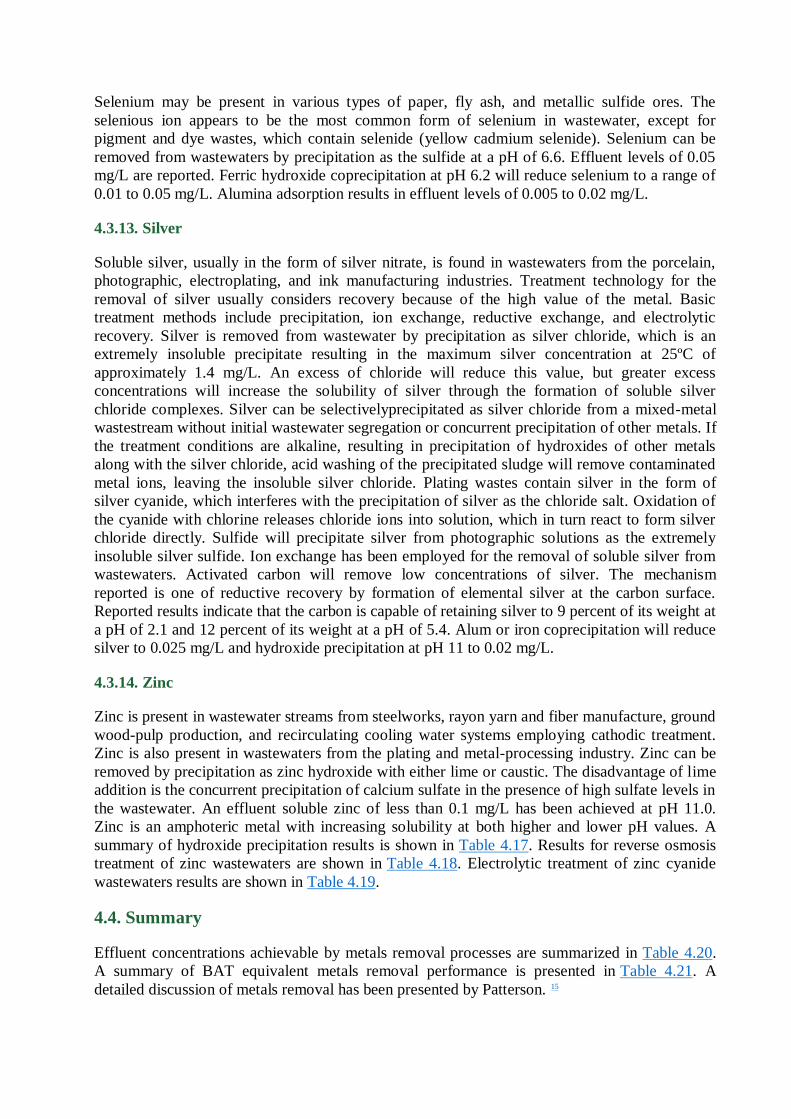
4.3.14. Zinc

Zinc is present in wastewater streams from steelworks, rayon yarn and fiber manufacture, ground

wood-pulp production, and recirculating cooling water systems employing cathodic treatment.

Zinc is also present in wastewaters from the plating and metal-processing industry. Zinc can be

removed by precipitation as zinc hydroxide with either lime or caustic. The disadvantage of lime

addition is the concurrent precipitation of calcium sulfate in the presence of high sulfate levels in

the wastewater. An effluent soluble zinc of less than 0.1 mg/L has been achieved at pH 11.0.

Zinc is an amphoteric metal with increasing solubility at both higher and lower pH values. A

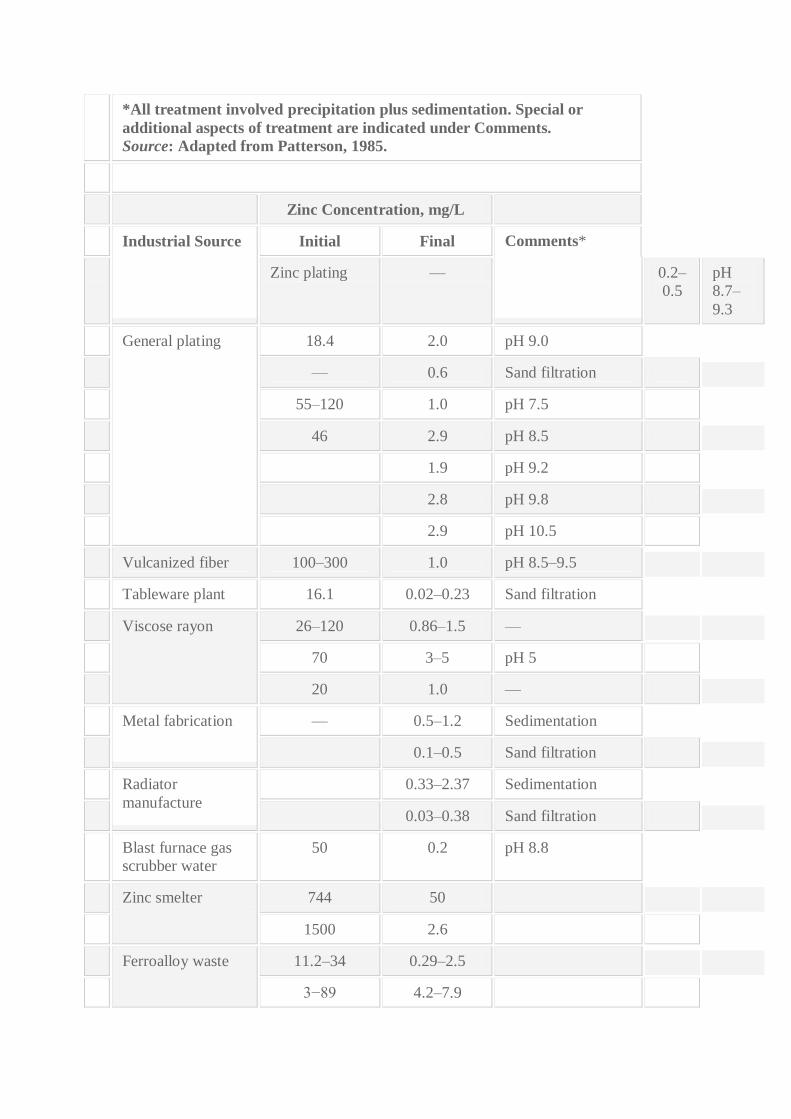
summary of hydroxide precipitation results is shown in Table 4.17. Results for reverse osmosis

treatment of zinc wastewaters are shown in Table 4.18. Electrolytic treatment of zinc cyanide

wastewaters results are shown in Table 4.19.

4.4. Summary

Effluent concentrations achievable by metals removal processes are summarized in Table 4.20.

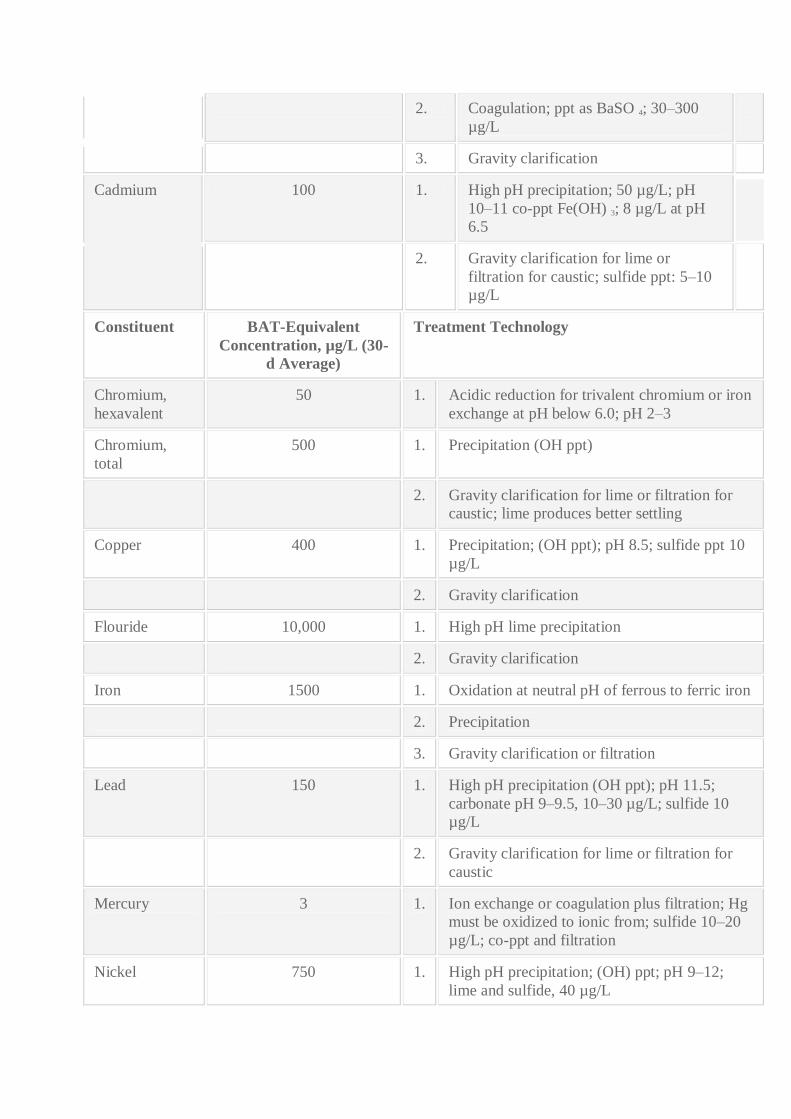
A summary of BAT equivalent metals removal performance is presented in Table 4.21. A

detailed discussion of metals removal has been presented by Patterson. 15

*All treatment involved precipitation plus sedimentation. Special or

additional aspects of treatment are indicated under Comments.

Source: Adapted from Patterson, 1985.

Zinc Concentration, mg/L

Industrial Source Initial Final Comments*

Zinc plating — 0.2–

0.5

pH

8.7–

9.3

General plating 18.4 2.0 pH 9.0

— 0.6 Sand filtration

55–120 1.0 pH 7.5

46 2.9 pH 8.5

1.9 pH 9.2

2.8 pH 9.8

2.9 pH 10.5

Vulcanized fiber 100–300 1.0 pH 8.5–9.5

Tableware plant 16.1 0.02–0.23 Sand filtration

Viscose rayon 26–120 0.86–1.5 —

70 3–5 pH 5

20 1.0 —

Metal fabrication — 0.5–1.2 Sedimentation

0.1–0.5 Sand filtration

Radiator

manufacture

0.33–2.37 Sedimentation

0.03–0.38 Sand filtration

Blast furnace gas

scrubber water

50 0.2 pH 8.8

Zinc smelter 744 50

1500 2.6

Ferroalloy waste 11.2–34 0.29–2.5

3−89 4.2–7.9

Ferrous foundry 72 1.26 Sedimentation

0.41 Sand filtration

Deep coal mine—

acid water

33–7.2 0.01–10

Source: Adapted from Cawley, 1980.

Zinc Concentration, μg/L

Industrial

Source

Feed Permeate % Removal

Zinc cyanide

plating rinse

1,700 30 98

Steam electric

power plant

300 53 82

780 3 99

Textile mill 7,200 140 98

5,400 6,600 −20

460 250 46

520 360 31

7,200 360 95

1,400 30 98

4,100 180 96

1,200 22 98

24,000 430 98

9,700 37 >99

Cooling tower

blowdown

10,000 300 97

Concentration, mg/L

Waste Parameter Initial Final

A Zinc 352 0.7

Cyanide 258 12.0

B Zinc 117 0.3

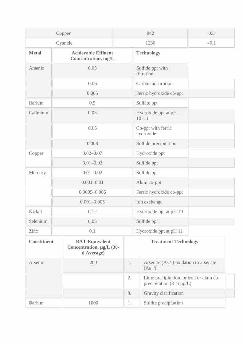
Copper 842 0.5

Cyanide 1230 <0.1

Metal Achievable Effluent

Concentration, mg/L

Technology

Arsenic 0.05 Sulfide ppt with

filtration

0.06 Carbon adsorption

0.005 Ferric hydroxide co-ppt

Barium 0.5 Sulfate ppt

Cadmium 0.05 Hydroxide ppt at pH

10–11

0.05 Co-ppt with ferric

hydroxide

0.008 Sulfide precipitation

Copper 0.02–0.07 Hydroxide ppt

0.01–0.02 Sulfide ppt

Mercury 0.01–0.02 Sulfide ppt

0.001–0.01 Alum co-ppt

0.0005–0.005 Ferric hydroxide co-ppt

0.001–0.005 Ion exchange

Nickel 0.12 Hydroxide ppt at pH 10

Selenium 0.05 Sulfide ppt

Zinc 0.1 Hydroxide ppt at pH 11

Constituent BAT-Equivalent

Concentration, µg/L (30-

d Average)

Treatment Technology

Arsenic 200 1. Arsenite (As +3) oxidation to arsenate

(As +5)

2. Lime precipitation, or iron or alum co-

precipitation (3–6 µg/L)

3. Gravity clarification

Barium 1000 1. Sulfite precipitation

2. Coagulation; ppt as BaSO 4; 30–300

µg/L

3. Gravity clarification

Cadmium 100 1. High pH precipitation; 50 µg/L; pH

10–11 co-ppt Fe(OH) 3; 8 µg/L at pH

6.5

2. Gravity clarification for lime or

filtration for caustic; sulfide ppt: 5–10

µg/L

Constituent BAT-Equivalent

Concentration, µg/L (30-

d Average)

Treatment Technology

Chromium,

hexavalent

50 1. Acidic reduction for trivalent chromium or iron

exchange at pH below 6.0; pH 2–3

Chromium,

total

500 1. Precipitation (OH ppt)

2. Gravity clarification for lime or filtration for

caustic; lime produces better settling

Copper 400 1. Precipitation; (OH ppt); pH 8.5; sulfide ppt 10

µg/L

2. Gravity clarification

Flouride 10,000 1. High pH lime precipitation

2. Gravity clarification

Iron 1500 1. Oxidation at neutral pH of ferrous to ferric iron

2. Precipitation

3. Gravity clarification or filtration

Lead 150 1. High pH precipitation (OH ppt); pH 11.5;

carbonate pH 9–9.5, 10–30 µg/L; sulfide 10

µg/L

2. Gravity clarification for lime or filtration for

caustic

Mercury 3 1. Ion exchange or coagulation plus filtration; Hg

must be oxidized to ionic from; sulfide 10–20

µg/L; co-ppt and filtration

Nickel 750 1. High pH precipitation; (OH) ppt; pH 9–12;

lime and sulfide, 40 µg/L

2. Gravity clarification and/or filtration

Silver 100 1. Ion exchange or ferric chloride co-precipitation

plus filtration

Zinc 500 1. Precipitation at optimized pH; Zn(OH) 2with

lime or caustic; pH 9–9.5 and 11

2. Gravity clarification and/or filtration

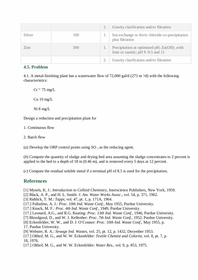
4.5. Problem

4.1. A metal-finishing plant has a wastewater flow of 72,000 gal/d (273 m 3/d) with the following

characteristics:

Cr 6+ 75 mg/L

Cu 10 mg/L

Ni 8 mg/L

Design a reduction and precipitation plant for

1. Continuous flow

2. Batch flow

(a) Develop the ORP control points using SO 2 as the reducing agent.

(b) Compute the quantity of sludge and drying bed area assuming the sludge concentrates to 2 percent is

applied to the bed to a depth of 18 in (0.46 m), and is removed every 5 days at 12 percent.

(c) Compute the residual soluble metal if a terminal pH of 8.5 is used for the precipitation.

References

[1] Mysels, K. J.: Introduction to Colloid Chemistry, Interscience Publishers, New York, 1959.

[2] Black, A. P., and H. L. Smith: J. Am. Water Works Assoc., vol. 54, p. 371, 1962.

[3] Riddick, T. M.: Tappi, vol. 47, pt. 1, p. 171A, 1964.

[17.] Palladino, A. J.: Proc. 10th Ind. Waste Conf., May 1955, Purdue University.

[17.] Knack, M. F.: Proc. 4th Ind. Waste Conf., 1949, Purdue University.

[17.] Leonard, A.G., and R.G. Keating: Proc. 13th Ind. Waste Conf., 1946, Purdue University.

[7] Bloodgood, D., and W. J. Kellenher: Proc. 7th Ind. Waste Conf., 1952, Purdue University.

[8] Eckenfelder, W. W., and D. J. O’Connor: Proc. 10th Ind. Waste Conf., May 1955, p.

17, Purdue University.

[9] Webster, R. A.: Sewage Ind. Wastes, vol. 25, pt. 12, p. 1432, December 1953.

[17.] Olthof, M. G., and W. W. Eckenfelder: Textile Chemist and Colorist, vol. 8, pt. 7, p.

18, 1976.

[17.] Olthof, M. G., and W. W. Eckenfelder: Water Res., vol. 9, p. 853, 1975.

[17.] Southgate, B. A.: Treatment and Disposal of Industrial Waste Waters, His Majesty’s

Stationery Office,London, 1948, p. 186.

[13] McCarthy, Joseph A.: Sewage Works J., vol. 21, pt. 1, p. 75, January 1949.

[14] Talinli, I.: Wat. Sci. Tech., 29, 9, p. 175, 1994.

[15] Patterson, J. W.: Industrial Wastewater Treatment Technology, Butterworth

Publishers, Boston, 1985.

[17.] Robinson, A., and J. Sum: U.S. EPA 600/2-80-139, June 1980.

[17.] Cawley, W. (ed.): Treatability Manual, vol. 3rd, U.S. EPA 600/8-80-042-C, July 1980.