Embed Size (px)
Citation preview
Draft chapter from An introduction to game theory by Martin J. Osborne. Version: 2002/7/[email protected]
http://www.economics.utoronto.ca/osborne
Copyright © 1995–2002 by Martin J. Osborne. All rights reserved. No part of this book may be re-produced by any electronic or mechanical means (including photocopying, recording, or informationstorage and retrieval) without permission in writing from Oxford University Press, except that onecopy of up to six chapters may be made by any individual for private study.
4Mixed Strategy Equilibrium
4.1 Introduction 97
4.2 Strategic games in which players may randomize 103
4.3 Mixed strategy Nash equilibrium 105
4.4 Dominated actions 117
4.5 Pure equilibria when randomization is allowed 120
4.6 Illustration: expert diagnosis 121
4.7 Equilibrium in a single population 126
4.8 Illustration: reporting a crime 128
4.9 The formation of players’ beliefs 132
4.10 Extension: Finding all mixed strategy Nash equilibria 135
4.11 Extension: Mixed equilibria of games in which each player has
a continuum of actions 140
4.12 Appendix: Representing preferences by expected
payoffs 144
Prerequisite: Chapter 2.
4.1 Introduction
4.1.1 Stochastic steady states
ANASH EQUILIBRIUM of a strategic game is an action profile in which everyplayer’s action is optimal given every other player’s action (Definition 21.1).
Such an action profile corresponds to a steady state of the idealized situation inwhich for each player in the game there is a population of individuals, and when-ever the game is played, one player is drawn randomly from each population (seeSection 2.6). In a steady state, every player’s behavior is the same whenever sheplays the game, and no player wishes to change her behavior, knowing (from herexperience) the other players’ behavior. In a steady state in which each player’s“behavior” is simply an action and within each population all players choose thesame action, the outcome of every play of the game is the same Nash equilibrium.
More general notions of a steady state allow the players’ choices to vary, aslong as the pattern of choices remains constant. For example, different members
97

98 Chapter 4. Mixed Strategy Equilibrium
of a given population may choose different actions, each player choosing the sameaction whenever she plays the game. Or each individual may, on each occasionshe plays the game, choose her action probabilistically according to the same, un-changing distribution. These two more general notions of a steady state are equiv-alent: a steady state of the first type in which the fraction p of the population rep-resenting player i chooses the action a corresponds to a steady state of the secondtype in which each member of the population representing player i chooses a withprobability p. In both cases, in each play of the game the probability that the indi-vidual in the role of player i chooses a is p. Both these notions of steady state aremodeled by a mixed strategy Nash equilibrium, a generalization of the notion ofNash equilibrium. For expository convenience, in most of this chapter I interpretsuch an equilibrium as a model of the second type of steady state, in which eachplayer chooses her actions probabilistically; such a steady state is called stochastic
(“involving probability”).
4.1.2 Example: Matching Pennies
An analysis of the game Matching Pennies (Example 17.1) illustrates the idea of astochastic steady state. My discussion focuses on the outcomes of this game, givenin Figure 98.1, rather than payoffs that represent the players’ preferences, as before.
Head Tail
Head $1, −$1 −$1, $1Tail −$1, $1 $1, −$1
Figure 98.1 The outcomes of Matching Pennies.
As we saw previously, this game has no Nash equilibrium: no pair of actions iscompatible with a steady state in which each player’s action is the same wheneverthe game is played. I claim, however, that the game has a stochastic steady state inwhich each player chooses each of her actions with probability 1
2 . To establish thisresult, I need to argue that if player 2 chooses each of her actions with probability 1
2 ,then player 1 optimally chooses each of her actions with probability 1
2 , and viceversa.
Suppose that player 2 chooses each of her actions with probability 12 . If player 1
chooses Head with probability p and Tail with probability 1 − p then each out-come (Head, Head) and (Head, Tail) occurs with probability 1
2 p, and each outcome(Tail, Head) and (Tail, Tail) occurs with probability 1
2 (1 − p). Thus player 1 gains$1 with probability 1
2 p + 12 (1 − p), which is equal to 1
2 , and loses $1 with proba-bility 1
2 . In particular, the probability distribution over outcomes is independentof p! Thus every value of p is optimal. In particular, player 1 can do no betterthan choose Head with probability 1
2 and Tail with probability 12 . A similar anal-
ysis shows that player 2 optimally chooses each action with probability 12 when

4.1 Introduction 99
player 1 does so. We conclude that the game has a stochastic steady state in whicheach player chooses each action with probability 1
2 .I further claim that, under a reasonable assumption on the players’ preferences,
the game has no other steady state. This assumption is that each player wants theprobability of her gaining $1 to be as large as possible. More precisely, if p > q theneach player prefers to gain $1 with probability p and lose $1 with probability 1 − p
than to gain $1 with probability q and lose $1 with probability 1 − q.To show that under this assumption there is no steady state in which the prob-
ability of each player’s choosing Head is different from 12 , denote the probability
with which player 2 chooses Head by q (so that she chooses Tail with probabil-ity 1 − q). If player 1 chooses Head with probability p then she gains $1 with prob-ability pq + (1 − p)(1 − q) (the probability that the outcome is either (Head, Head)
or (Tail, Tail)) and loses $1 with probability (1 − p)q + p(1 − q). The first probabil-ity is equal to 1 − q + p(2q − 1) and the second is equal to q + p(1 − 2q). Thus ifq < 1
2 (player 2 chooses Head with probability less than 12 ), the first probability is
decreasing in p and the second is increasing in p, so that the lower is p, the betteris the outcome for player 1; the value of p that induces the best probability dis-tribution over outcomes for player 1 is 0. That is, if player 2 chooses Head withprobability less than 1
2 , then the uniquely best policy for player 1 is to choose Tail
with certainty. A similar argument shows that if player 2 chooses Head with prob-ability greater than 1
2 , the uniquely best policy for player 1 is to choose Head withcertainty.
Now, if player 1 chooses one of her actions with certainty, an analysis like that inthe previous paragraph leads to the conclusion that the optimal policy of player 2is to choose one of her actions with certainty (Head if player 1 chooses Tail and Tail
if player 1 chooses Head).We conclude that there is no steady state in which the probability that player 2
chooses Head is different from 12 . A symmetric argument leads to the conclusion
that there is no steady state in which the probability that player 1 chooses Head isdifferent from 1
2 . Thus the only stochastic steady state is that in which each playerchooses each of her actions with probability 1
2 .As discussed in the first section, the stable pattern of behavior we have found
can be alternatively interpreted as a steady state in which no player randomizes.Instead, half the players in the population of individuals who take the role ofplayer 1 in the game choose Head whenever they play the game and half of themchoose Tail whenever they play the game; similarly half of those who take therole of player 2 choose Head and half choose Tail. Given that the individuals in-volved in any given play of the game are chosen randomly from the populations,in each play of the game each individual faces with probability 1
2 an opponent whochooses Head, and with probability 1
2 an opponent who chooses Tail.
? EXERCISE 99.1 (Variant of Matching Pennies) Find the steady state(s) of the gamethat differs from Matching Pennies only in that the outcomes of (Head,Head) and of(Tail,Tail) are that player 1 gains $2 and player 2 loses $1.
100 Chapter 4. Mixed Strategy Equilibrium
4.1.3 Generalizing the analysis: expected payoffs
The fact that Matching Pennies has only two outcomes for each player (gain $1, lose$1) makes the analysis of a stochastic steady state particularly simple, because itallows us to deduce, under a weak assumption, the players’ preferences regardinglotteries (probability distributions) over outcomes from their preferences regardingdeterministic outcomes (outcomes that occur with certainty). If a player prefersthe deterministic outcome a to the deterministic outcome b, it is very plausible thatif p > q then she prefers the lottery in which a occurs with probability p (and b
occurs with probability 1 − p) to the lottery in which a occurs with probability q
(and b occurs with probability 1 − q).In a game with more than two outcomes for some player, we cannot extrapo-
late in this way from preferences regarding deterministic outcomes to preferencesregarding lotteries over outcomes. Suppose, for example, that a game has threepossible outcomes, a, b, and c, and that a player prefers a to b to c. Does she preferthe deterministic outcome b to the lottery in which a and c each occur with prob-ability 1
2 , or vice versa? The information about her preferences over deterministicoutcomes gives us no clue about the answer to this question. She may prefer b
to the lottery in which a and c each occur with probability 12 , or she may prefer
this lottery to b; both preferences are consistent with her preferring a to b to c. Inorder to study her behavior when she is faced with choices between lotteries, weneed to add to the model a description of her preferences regarding lotteries overoutcomes.
A standard assumption in game theory restricts attention to preferences regard-ing lotteries over outcomes that may be represented by the expected value of a pay-off function over deterministic outcomes. (See Section 17.6.3 if you are unfamiliarwith the notion of “expected value”.) That is, for every player i there is a payofffunction ui with the property that player i prefers one lottery over outcomes to an-other if and only if, according to ui, the expected value of the first lottery exceedsthe expected value of the second lottery.
For example, suppose that there are three outcomes, a, b, and c, and lottery P
yields a with probability pa, b with probability pb, and c with probability pc, whereaslottery Q yields these three outcomes with probabilities qa, qb, and qc. Then the as-sumption is that for each player i there are numbers ui(a), ui(b), and ui(c) such thatplayer i prefers lottery P to lottery Q if and only if paui(a) + pbui(b) + pcui(c) >
qaui(a) + qbui(b) + qcui(c). (I discuss the representation of preferences by the ex-pected value of a payoff function in more detail in Section 4.12, an appendix to thischapter.)
The first systematic investigation of preferences regarding lotteries representedby the expected value of a payoff function over deterministic outcomes was un-dertaken by von Neumann and Morgenstern (1944). Accordingly such preferencesare called vNM preferences. A payoff function over deterministic outcomes (ui
in the previous paragraph) whose expected value represents such preferences iscalled a Bernoulli payoff function (in honor of Daniel Bernoulli (1700–1782), who
4.1 Introduction 101
appears to have been one of the first persons to use such a function to representpreferences).
The restrictions on preferences regarding deterministic outcomes required forthem to be represented by a payoff function are relatively innocuous (see Sec-tion 1.2.2). The same is not true of the restrictions on preferences regarding lot-teries over outcomes required for them to be represented by the expected value ofa payoff function. (I do not discuss these restrictions, but the box at the end of thissection gives an example of preferences that violate them.) Nevertheless, we ob-tain many insights from models that assume preferences take this form; followingstandard game theory (and standard economic theory), I maintain the assumptionthroughout the book.
The assumption that a player’s preferences be represented by the expectedvalue of a payoff function does not restrict her attitudes to risk: a person whosepreferences are represented by such a function may have an arbitrarily strong likeor dislike for risk. Suppose, for example, that a, b, and c are three outcomes, and aperson prefers a to b to c. A person who is very averse to risky outcomes prefers toobtain b for sure rather than to face the lottery in which a occurs with probability p
and c occurs with probability 1 − p, even if p is relatively large. Such preferencesmay be represented by the expected value of a payoff function u for which u(a) isclose to u(b), which is much larger than u(c). A person who is not at all averse torisky outcomes prefers the lottery to the certain outcome b, even if p is relativelysmall. Such preferences are represented by the expected value of a payoff functionu for which u(a) is much larger than u(b), which is close to u(c). If u(a) = 10,u(b) = 9, and u(c) = 0, for example, then the person prefers the certain outcomeb to any lottery between a and c that yields a with probability less than 9
10 . But ifu(a) = 10, u(b) = 1, and u(c) = 0, she prefers any lottery between a and c thatyields a with probability greater than 1
10 to the certain outcome b.Suppose that the outcomes are amounts of money and a person’s preferences
are represented by the expected value of a payoff function in which the payoff ofeach outcome is equal to the amount of money involved. Then we say the person isrisk neutral. Such a person compares lotteries according to the expected amount ofmoney involved. (For example, she is indifferent between receiving $100 for sureand the lottery that yields $0 with probability 9
10 and $1000 with probability 110 .)
On the one hand, the fact that people buy insurance suggests that in some circum-stances preferences are risk averse: people prefer to obtain $z with certainty thanto receive the outcome of a lottery that yields $z on average. On the other hand,the fact that people buy lottery tickets that pay, on average, much less than theirpurchase price, suggests that in other circumstances preferences are risk preferring.In both cases, preferences over lotteries are not represented by expected monetary
values, though they still may be represented by the expected value of a payoff func-tion (in which the payoffs to outcome are different from the monetary values of theoutcomes).
Any given preferences over deterministic outcomes are represented by manydifferent payoff functions (see Section 1.2.2). The same is true of preferences over

102 Chapter 4. Mixed Strategy Equilibrium
lotteries; the relation between payoff functions whose expected values representthe same preferences is discussed in Section 4.12.2 in the appendix to this chap-ter. In particular, we may choose arbitrary payoffs for the outcomes that are bestand worst according to the preferences, as long as the payoff to the best outcomeexceeds the payoff to the worst outcome. For example, suppose there are threeoutcomes, a, b, and c, and a person prefers a to b to c, and is indifferent between b
and the lottery that yields a with probability 12 and c with probability 1
2 . Then wemay choose u(a) = 3 and u(c) = 1, in which case u(b) = 2; or, for example, wemay choose u(a) = 10 and u(c) = 0, in which case u(b) = 5.
SOME EVIDENCE ON EXPECTED PAYOFF FUNCTIONS
Consider the following two lotteries (the first of which is, in fact, deterministic):
Lottery 1 You receive $2 million with certainty
Lottery 2 You receive $10 million with probability 0.1, $2 million with probabil-ity 0.89, and nothing with probability 0.01.
Which do you prefer? Now consider two more lotteries:
Lottery 3 You receive $2 million with probability 0.11 and nothing with probabil-ity 0.89
Lottery 4 You receive $10 million with probability 0.1 and nothing with probabil-ity 0.9.
Which do you prefer? A significant fraction of experimental subjects say they pre-fer lottery 1 to lottery 2, and lottery 4 to lottery 3. (See, for example, Conlisk (1989)and Camerer (1995, 622–623).)
These preferences cannot be represented by an expected payoff function! Ifthey could be, there would exist a payoff function u for which the expected payoffof lottery 1 exceeds that of lottery 2:
u(2) > 0.1u(10) + 0.89u(2) + 0.01u(0),
where the amounts of money are expressed in millions. Subtracting 0.89u(2) andadding 0.89u(0) to each side we obtain
0.11u(2) + 0.89u(0) > 0.1u(10) + 0.9u(0).
But this inequality says that the expected payoff of lottery 3 exceeds that of lot-tery 4! Thus preferences represented by an expected payoff function that yield apreference for lottery 1 over lottery 2 must also yield a preference for lottery 3 overlottery 4.
Preferences represented by the expected value of a payoff function are, how-

4.2 Strategic games in which players may randomize 103
ever, consistent with a person’s being indifferent between lotteries 1 and 2, andbetween lotteries 3 and 4. Suppose we assume that when a person is almost in-different between two lotteries, she may make a “mistake”. Then a person’s ex-pressed preference for lottery 1 over lottery 2 and for lottery 4 over lottery 3 is notdirectly inconsistent with her preferences being represented by the expected valueof a payoff function in which she is almost indifferent between lotteries 1 and 2 andbetween lotteries 3 and 4. If, however, we add the assumption that mistakes aredistributed symmetrically, then the frequency with which people express a prefer-ence for lottery 2 over lottery 1 and for lottery 4 over lottery 3 (also inconsistentwith preferences represented by the expected value of a payoff function) should besimilar to that with which people express a preference for lottery 1 over lottery 2and for lottery 3 over lottery 4. In fact, however, the second pattern is significantlymore common than the first (Conlisk 1989), so that a more significant modificationof the theory is needed to explain the observations.
A limitation of the evidence is that it is based on the preferences expressedby people faced with hypothetical choices; understandably (given the amounts ofmoney involved), no experiment has been run in which subjects were paid accord-ing to the lotteries they chose! Experiments with stakes consistent with normalresearch budgets show few choices inconsistent with preferences represented bythe expected value of a payoff function (Conlisk 1989). This evidence, however,does not contradict the evidence based on hypothetical choices with large stakes:with larger stakes subjects might make choices in line with the preferences theyexpress when asked about hypothetical choices.
In summary, the evidence for an inconsistency with preferences compatiblewith an expected payoff function is, at a minimum, suggestive. It has spurredthe development of alternative theories. Nevertheless, the vast majority of mod-els in game theory (and also in economics) that involve choice under uncertaintycurrently assume that each decision-maker’s preferences are represented by theexpected value of a payoff function. I maintain this assumption throughout thebook, although many of the ideas I discuss appear not to depend on it.
4.2 Strategic games in which players may randomize
To study stochastic steady states, we extend the notion of a strategic game givenin Definition 11.1 by endowing each player with vNM preferences about lotteriesover the set of action profiles.
I DEFINITION 103.1 (Strategic game with vNM preferences) A strategic game (withvNM preferences) consists of
• a set of players
• for each player, a set of actions
104 Chapter 4. Mixed Strategy Equilibrium
• for each player, preferences regarding lotteries over action profiles that maybe represented by the expected value of a (“Bernoulli”) payoff function overaction profiles.
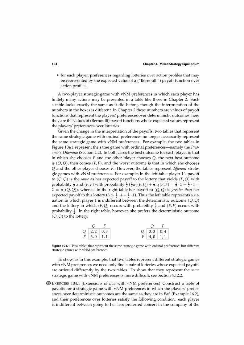
A two-player strategic game with vNM preferences in which each player hasfinitely many actions may be presented in a table like those in Chapter 2. Sucha table looks exactly the same as it did before, though the interpretation of thenumbers in the boxes is different. In Chapter 2 these numbers are values of payofffunctions that represent the players’ preferences over deterministic outcomes; herethey are the values of (Bernoulli) payoff functions whose expected values representthe players’ preferences over lotteries.
Given the change in the interpretation of the payoffs, two tables that representthe same strategic game with ordinal preferences no longer necessarily representthe same strategic game with vNM preferences. For example, the two tables inFigure 104.1 represent the same game with ordinal preferences—namely the Pris-
oner’s Dilemma (Section 2.2). In both cases the best outcome for each player is thatin which she chooses F and the other player chooses Q, the next best outcomeis (Q, Q), then comes (F, F), and the worst outcome is that in which she choosesQ and the other player chooses F. However, the tables represent different strate-gic games with vNM preferences. For example, in the left table player 1’s payoffto (Q, Q) is the same as her expected payoff to the lottery that yields (F, Q) withprobability 1
2 and (F, F) with probability 12 ( 1
2 u1(F, Q) + 12 u1(F, F) = 1
2 · 3 + 12 · 1 =
2 = u1(Q, Q)), whereas in the right table her payoff to (Q, Q) is greater than herexpected payoff to this lottery (3 > 1
2 · 4 + 12 · 1). Thus the left table represents a sit-
uation in which player 1 is indifferent between the deterministic outcome (Q, Q)
and the lottery in which (F, Q) occurs with probability 12 and (F, F) occurs with
probability 12 . In the right table, however, she prefers the deterministic outcome
(Q, Q) to the lottery.
Q F
Q 2, 2 0, 3F 3, 0 1, 1
Q F
Q 3, 3 0, 4F 4, 0 1, 1
Figure 104.1 Two tables that represent the same strategic game with ordinal preferences but differentstrategic games with vNM preferences.
To show, as in this example, that two tables represent different strategic gameswith vNM preferences we need only find a pair of lotteries whose expected payoffsare ordered differently by the two tables. To show that they represent the same
strategic game with vNM preferences is more difficult; see Section 4.12.2.
? EXERCISE 104.1 (Extensions of BoS with vNM preferences) Construct a table ofpayoffs for a strategic game with vNM preferences in which the players’ prefer-ences over deterministic outcomes are the same as they are in BoS (Example 16.2),and their preferences over lotteries satisfy the following condition: each playeris indifferent between going to her less preferred concert in the company of the

4.3 Mixed strategy Nash equilibrium 105
other player and the lottery in which with probability 12 she and the other player
go to different concerts and with probability 12 they both go to her more preferred
concert. Do the same in the case that each player is indifferent between goingto her less preferred concert in the company of the other player and the lotteryin which with probability 3
4 she and the other player go to different concerts andwith probability 1
4 they both go to her more preferred concert. (In each case seteach player’s payoff to the outcome that she least prefers equal to 0 and her payoffto the outcome that she most prefers equal to 2.)
Despite the importance of saying how the numbers in a payoff table shouldbe interpreted, users of game theory sometimes fail to make the interpretationclear. When interpreting discussions of Nash equilibrium in the literature, a rea-sonably safe assumption is that if the players are not allowed to choose their ac-tions randomly then the numbers in payoff tables are payoffs that represent theplayers’ ordinal preferences, whereas if the players are allowed to randomize thenthe numbers are payoffs whose expected values represent the players’ preferencesregarding lotteries over outcomes.
4.3 Mixed strategy Nash equilibrium
4.3.1 Mixed strategies
In the generalization of the notion of Nash equilibrium that models a stochasticsteady state of a strategic game with vNM preferences, we allow each player tochoose a probability distribution over her set of actions rather than restricting herto choose a single deterministic action. We refer to such a probability distributionas a mixed strategy.
I DEFINITION 105.1 (Mixed strategy) A mixed strategy of a player in a strategic gameis a probability distribution over the player’s actions.
I usually use α to denote a profile of mixed strategies; αi(ai) is the probabilityassigned by player i’s mixed strategy αi to her action ai. To specify a mixed strategyof player i we need to give the probability it assigns to each of player i’s actions.For example, the strategy of player 1 in Matching Pennies that assigns probability 1
2to each action is the strategy α1 for which α1(Head) = 1
2 and α1(Tail) = 12 . Because
this way of describing a mixed strategy is cumbersome, I often use a shorthandfor a game that is presented in a table like those in Figure 104.1: I write a mixedstrategy as a list of probabilities, one for each action, in the order the actions are given
in the table. For example, the mixed strategy ( 13 , 2
3 ) for player 1 in either of thegames in Figure 104.1 assigns probability 1
3 to Q and probability 23 to F.
A mixed strategy may assign probability 1 to a single action: by allowing aplayer to choose probability distributions, we do not prohibit her from choos-ing deterministic actions. We refer to such a mixed strategy as a pure strategy.Player i’s choosing the pure strategy that assigns probability 1 to the action ai is
106 Chapter 4. Mixed Strategy Equilibrium
equivalent to her simply choosing the action ai, and I denote this strategy simplyby ai.
4.3.2 Equilibrium
The notion of equilibrium that we study is called “mixed strategy Nash equilib-rium”. The idea behind it is the same as the idea behind the notion of Nash equi-librium for a game with ordinal preferences: a mixed strategy Nash equilibrium isa mixed strategy profile α∗ with the property that no player i has a mixed strategyαi such that she prefers the lottery over outcomes generated by the strategy pro-file (αi, α∗
−i) to the lottery over outcomes generated by the strategy profile α∗. Thefollowing definition gives this condition using payoff functions whose expectedvalues represent the players’ preferences.
I DEFINITION 106.1 (Mixed strategy Nash equilibrium of strategic game with vNM pref-
erences) The mixed strategy profile α∗ in a strategic game with vNM preferences isa (mixed strategy) Nash equilibrium if, for each player i and every mixed strategyαi of player i, the expected payoff to player i of α∗ is at least as large as the expectedpayoff to player i of (αi, α∗
−i) according to a payoff function whose expected valuerepresents player i’s preferences over lotteries. Equivalently, for each player i,
Ui(α∗) ≥ Ui(αi, α∗−i) for every mixed strategy αi of player i, (106.2)
where Ui(α) is player i’s expected payoff to the mixed strategy profile α.
4.3.3 Best response functions
When studying mixed strategy Nash equilibria, as when studying Nash equilibriaof strategic games with ordinal preferences, the players’ best response functions(Section 2.8) are often useful. As before, I denote player i’s best response functionby Bi. For a strategic game with ordinal preferences, Bi(a−i) is the set of player i’sbest actions when the list of the other players’ actions is a−i. For a strategic gamewith vNM preferences, Bi(α−i) is the set of player i’s best mixed strategies whenthe list of the other players’ mixed strategies is α−i. From the definition of a mixedstrategy equilibrium, a profile α∗ of mixed strategies is a mixed strategy Nash equi-librium if and only if every player’s mixed strategy is a best response to the otherplayers’ mixed strategies (cf. Proposition 34.1):
the mixed strategy profile α∗ is a mixed strategy Nash equilibrium if and
only if α∗i is in Bi(α∗
−i) for every player i.
4.3.4 Best response functions in two-player two-action games
The analysis of Matching Pennies in Section 4.1.2 shows that each player’s set ofbest responses to the other player’s mixed strategy is either a single pure strategyor the set of all mixed strategies. (For example, if player 2’s mixed strategy assigns
4.3 Mixed strategy Nash equilibrium 107
probability less than 12 to Head then player 1’s unique best response is the pure
strategy Tail, if player 2’s mixed strategy assigns probability greater than 12 to Head
then player 1’s unique best response is the pure strategy Head, and if player 2’smixed strategy assigns probability 1
2 to Head then all of player 1’s mixed strategiesare best responses.)
In any two-player game in which each player has two actions, the set of eachplayer’s best responses has a similar character: it consists either of a single purestrategy, or of all mixed strategies. The reason lies in the form of the payoff func-tions.
Consider a two-player game in which each player has two actions, T and B forplayer 1 and L and R for player 2. Denote by ui, for i = 1, 2, a Bernoulli payofffunction for player i. (That is, ui is a payoff function over action pairs whose ex-pected value represents player i’s preferences regarding lotteries over action pairs.)Player 1’s mixed strategy α1 assigns probability α1(T) to her action T and probabil-ity α1(B) to her action B (with α1(T) + α1(B) = 1). For convenience, let p = α1(T),so that α1(B) = 1 − p. Similarly, denote the probability α2(L) that player 2’s mixedstrategy assigns to L by q, so that α2(R) = 1 − q.
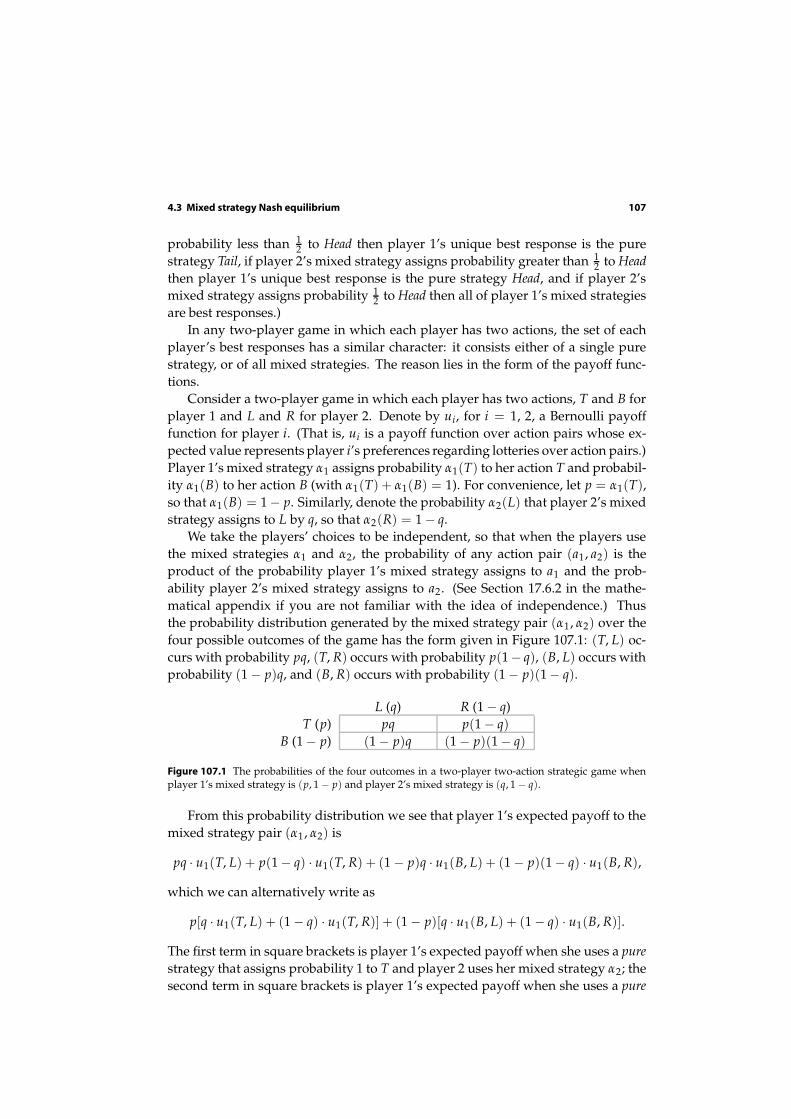
We take the players’ choices to be independent, so that when the players usethe mixed strategies α1 and α2, the probability of any action pair (a1, a2) is theproduct of the probability player 1’s mixed strategy assigns to a1 and the prob-ability player 2’s mixed strategy assigns to a2. (See Section 17.6.2 in the mathe-matical appendix if you are not familiar with the idea of independence.) Thusthe probability distribution generated by the mixed strategy pair (α1, α2) over thefour possible outcomes of the game has the form given in Figure 107.1: (T, L) oc-curs with probability pq, (T, R) occurs with probability p(1− q), (B, L) occurs withprobability (1 − p)q, and (B, R) occurs with probability (1 − p)(1 − q).
L (q) R (1 − q)T (p) pq p(1 − q)
B (1 − p) (1 − p)q (1 − p)(1 − q)
Figure 107.1 The probabilities of the four outcomes in a two-player two-action strategic game whenplayer 1’s mixed strategy is (p, 1 − p) and player 2’s mixed strategy is (q, 1 − q).
From this probability distribution we see that player 1’s expected payoff to themixed strategy pair (α1, α2) is
pq · u1(T, L) + p(1 − q) · u1(T, R) + (1 − p)q · u1(B, L) + (1 − p)(1 − q) · u1(B, R),
which we can alternatively write as
p[q · u1(T, L) + (1 − q) · u1(T, R)] + (1 − p)[q · u1(B, L) + (1 − q) · u1(B, R)].
The first term in square brackets is player 1’s expected payoff when she uses a pure
strategy that assigns probability 1 to T and player 2 uses her mixed strategy α2; thesecond term in square brackets is player 1’s expected payoff when she uses a pure
108 Chapter 4. Mixed Strategy Equilibrium
strategy that assigns probability 1 to B and player 2 uses her mixed strategy α2. De-note these two expected payoffs E1(T, α2) and E1(B, α2). Then player 1’s expectedpayoff to the mixed strategy pair (α1, α2) is
pE1(T, α2) + (1 − p)E1(B, α2).
That is, player 1’s expected payoff to the mixed strategy pair (α1, α2) is a weightedaverage of her expected payoffs to T and B when player 2 uses the mixed strat-egy α2, with weights equal to the probabilities assigned to T and B by α1.
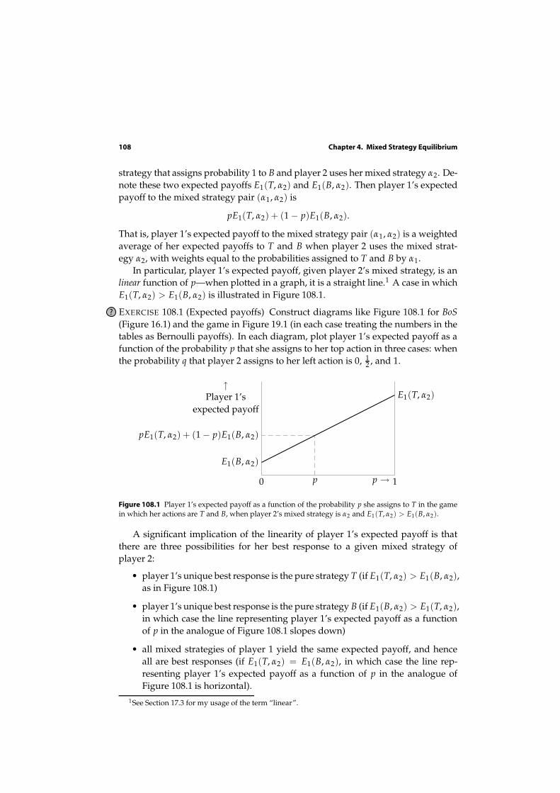
In particular, player 1’s expected payoff, given player 2’s mixed strategy, is anlinear function of p—when plotted in a graph, it is a straight line.1 A case in whichE1(T, α2) > E1(B, α2) is illustrated in Figure 108.1.
? EXERCISE 108.1 (Expected payoffs) Construct diagrams like Figure 108.1 for BoS
(Figure 16.1) and the game in Figure 19.1 (in each case treating the numbers in thetables as Bernoulli payoffs). In each diagram, plot player 1’s expected payoff as afunction of the probability p that she assigns to her top action in three cases: whenthe probability q that player 2 assigns to her left action is 0, 1
2 , and 1.
↑Player 1’s
expected payoff
E1(B, α2)
E1(T, α2)
0 1p →
pE1(T, α2) + (1 − p)E1(B, α2)
p
Figure 108.1 Player 1’s expected payoff as a function of the probability p she assigns to T in the gamein which her actions are T and B, when player 2’s mixed strategy is α2 and E1(T, α2) > E1(B, α2).
A significant implication of the linearity of player 1’s expected payoff is thatthere are three possibilities for her best response to a given mixed strategy ofplayer 2:
• player 1’s unique best response is the pure strategy T (if E1(T, α2) > E1(B, α2),as in Figure 108.1)
• player 1’s unique best response is the pure strategy B (if E1(B, α2) > E1(T, α2),in which case the line representing player 1’s expected payoff as a functionof p in the analogue of Figure 108.1 slopes down)
• all mixed strategies of player 1 yield the same expected payoff, and henceall are best responses (if E1(T, α2) = E1(B, α2), in which case the line rep-resenting player 1’s expected payoff as a function of p in the analogue ofFigure 108.1 is horizontal).
1See Section 17.3 for my usage of the term “linear”.

4.3 Mixed strategy Nash equilibrium 109
In particular, a mixed strategy (p, 1 − p) for which 0 < p < 1 is never the unique
best response; either it is not a best response, or all mixed strategies are best re-sponses.
? EXERCISE 109.1 (Best responses) For each game and each value of q in Exercise 108.1,use the graphs you drew in that exercise to find player 1’s set of best responses.
4.3.5 Example: Matching Pennies
The argument in Section 4.1.2 establishes that Matching Pennies has a unique mixedstrategy Nash equilibrium, in which each player’s mixed strategy assigns proba-bility 1
2 to Head and probability 12 to Tail. I now describe an alternative route to this
conclusion that uses the method described in Section 2.8.3, which involves explic-itly constructing the players’ best response functions; this method may be used inother games.
Represent each player’s preferences by the expected value of a payoff functionthat assigns the payoff 1 to a gain of $1 and the payoff −1 to a loss of $1. Theresulting strategic game with vNM preferences is shown in Figure 109.1.
Head Tail
Head 1, −1 −1, 1Tail −1, 1 1, −1
Figure 109.1 Matching Pennies.
Denote by p the probability that player 1’s mixed strategy assigns to Head, andby q the probability that player 2’s mixed strategy assigns to Head. Then, givenplayer 2’s mixed strategy, player 1’s expected payoff to the pure strategy Head is
q · 1 + (1 − q) · (−1) = 2q − 1
and her expected payoff to Tail is
q · (−1) + (1 − q) · 1 = 1 − 2q.
Thus if q < 12 then player 1’s expected payoff to Tail exceeds her expected payoff
to Head, and hence exceeds also her expected payoff to every mixed strategy thatassigns a positive probability to Head. Similarly, if q > 1
2 then her expected payoffto Head exceeds her expected payoff to Tail, and hence exceeds her expected payoffto every mixed strategy that assigns a positive probability to Tail. If q = 1
2 thenboth Head and Tail, and hence all her mixed strategies, yield the same expectedpayoff. We conclude that player 1’s best responses to player 2’s strategy are hermixed strategy that assigns probability 0 to Head if q < 1
2 , her mixed strategy thatassigns probability 1 to Head if q > 1
2 , and all her mixed strategies if q = 12 . That is,
denoting by B1(q) the set of probabilities player 1 assigns to Head in best responses
110 Chapter 4. Mixed Strategy Equilibrium
to q, we have
B1(q) =
{0} if q < 12
{p: 0 ≤ p ≤ 1} if q = 12
{1} if q > 12 .
The best response function of player 2 is similar: B2(p) = {1} if p < 12 , B2(p) =
{q: 0 ≤ q ≤ 1} if p = 12 , and B2(p) = {0} if p > 1
2 . Both best response functions areillustrated in Figure 110.1.
0 12
1p →
12
1↑q
B1
B2
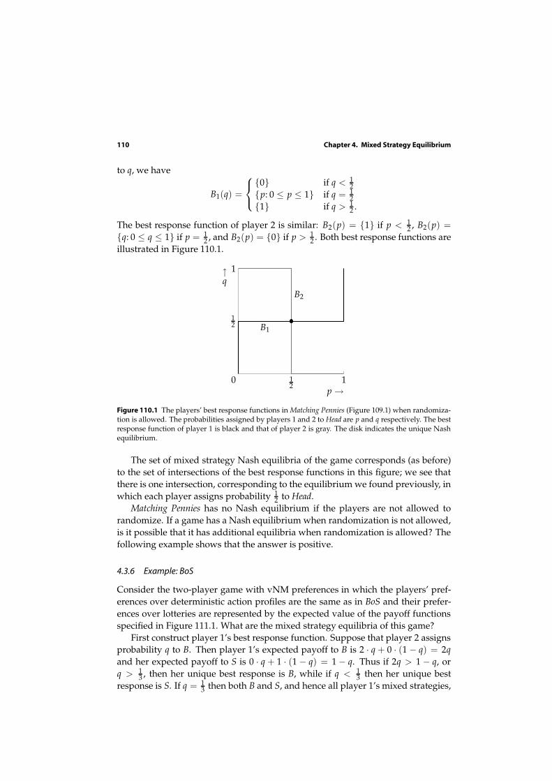
Figure 110.1 The players’ best response functions in Matching Pennies (Figure 109.1) when randomiza-tion is allowed. The probabilities assigned by players 1 and 2 to Head are p and q respectively. The bestresponse function of player 1 is black and that of player 2 is gray. The disk indicates the unique Nashequilibrium.
The set of mixed strategy Nash equilibria of the game corresponds (as before)to the set of intersections of the best response functions in this figure; we see thatthere is one intersection, corresponding to the equilibrium we found previously, inwhich each player assigns probability 1
2 to Head.Matching Pennies has no Nash equilibrium if the players are not allowed to
randomize. If a game has a Nash equilibrium when randomization is not allowed,is it possible that it has additional equilibria when randomization is allowed? Thefollowing example shows that the answer is positive.
4.3.6 Example: BoS
Consider the two-player game with vNM preferences in which the players’ pref-erences over deterministic action profiles are the same as in BoS and their prefer-ences over lotteries are represented by the expected value of the payoff functionsspecified in Figure 111.1. What are the mixed strategy equilibria of this game?
First construct player 1’s best response function. Suppose that player 2 assignsprobability q to B. Then player 1’s expected payoff to B is 2 · q + 0 · (1 − q) = 2q
and her expected payoff to S is 0 · q + 1 · (1 − q) = 1 − q. Thus if 2q > 1 − q, orq > 1
3 , then her unique best response is B, while if q < 13 then her unique best
response is S. If q = 13 then both B and S, and hence all player 1’s mixed strategies,

4.3 Mixed strategy Nash equilibrium 111
B S
B 2, 1 0, 0S 0, 0 1, 2
Figure 111.1 A version of the game BoS with vNM preferences.
0 23
1p →
13
1↑q
B1
B2
Figure 111.2 The players’ best response functions in BoS (Figure 111.1) when randomization is allowed.The probabilities assigned by players 1 and 2 to B are p and q respectively. The best response functionof player 1 is black and that of player 2 is gray. The disks indicate the Nash equilibria (two pure, onemixed).
yield the same expected payoffs, so that every mixed strategy is a best response.In summary, player 1’s best response function is
B1(q) =
{0} if q < 13
{p : 0 ≤ p ≤ 1} if q = 13
{1} if q > 13 .
Similarly we can find player 2’s best response function. The best response func-tions of both players are shown in Figure 111.2.
We see that the game has three mixed strategy Nash equilibria, in which (p, q) =
(0, 0), ( 23 , 1
3 ), and (1, 1). The first and third equilibria correspond to the Nash equi-libria of the ordinal version of the game when the players were not allowed torandomize (Section 2.7.2). The second equilibrium is new. In this equilibrium eachplayer chooses both B and S with positive probability (so that each of the fouroutcomes (B, B), (B, S), (S, B), and (S, S) occurs with positive probability).
? EXERCISE 111.1 (Mixed strategy equilibria of Hawk–Dove) Consider the two-playergame with vNM preferences in which the players’ preferences over determinis-tic action profiles are the same as in Hawk–Dove (Exercise 29.2) and their prefer-ences over lotteries satisfy the following two conditions. Each player is indifferentbetween the outcome (Passive, Passive) and the lottery that assigns probability 1
2to (Aggressive, Aggressive) and probability 1
2 to the outcome in which she is ag-gressive and the other player is passive, and between the outcome in which she

112 Chapter 4. Mixed Strategy Equilibrium
is passive and the other player is aggressive and the lottery that assigns proba-bility 2
3 to the outcome (Aggressive, Aggressive) and probability 13 to the outcome
(Passive, Passive). Find payoffs whose expected values represent these preferences(take each player’s payoff to (Aggressive, Aggressive) to be 0 and each player’s pay-off to the outcome in which she is passive and the other player is aggressive to be1). Find the mixed strategy Nash equilibrium of the resulting strategic game.
Both Matching Pennies and BoS have finitely many mixed strategy Nash equi-libria: the players’ best response functions intersect at a finite number of points(one for Matching Pennies, three for BoS). One of the games in the next exercise hasa continuum of mixed strategy Nash equilibria because segments of the players’best response functions coincide.
? EXERCISE 112.1 (Games with mixed strategy equilibria) Find all the mixed strategyNash equilibria of the strategic games in Figure 112.1.
L R
T 6, 0 0, 6B 3, 2 6, 0
L R
T 0, 1 0, 2B 2, 2 0, 1
Figure 112.1 Two strategic games with vNM preferences.
? EXERCISE 112.2 (A coordination game) Two people can perform a task if, and onlyif, they both exert effort. They are both better off if they both exert effort and per-form the task than if neither exerts effort (and nothing is accomplished); the worstoutcome for each person is that she exerts effort and the other does not (in whichcase again nothing is accomplished). Specifically, the players’ preferences are rep-resented by the expected value of the payoff functions in Figure 112.2, where c isa positive number less than 1 that can be interpreted as the cost of exerting effort.Find all the mixed strategy Nash equilibria of this game. How do the equilibriachange as c increases? Explain the reasons for the changes.
No effort Effort
No effort 0, 0 0, −c
Effort −c, 0 1 − c, 1 − c
Figure 112.2 The coordination game in Exercise 112.2.
?? EXERCISE 112.3 (Swimming with sharks) You and a friend are spending two daysat the beach; both of you enjoy swimming. Each of you believes that with probabil-ity π the water is infested with sharks. If sharks are present, a swimmer will surelybe attacked. Each of you has preferences represented by the expected value of apayoff function that assigns −c to being attacked by a shark (where c > 0!), 0 to sit-ting on the beach, and 1 to a day’s worth of undisturbed swimming. If a swimmer

4.3 Mixed strategy Nash equilibrium 113
is attacked by sharks on the first day then you both deduce that a swimmer willsurely be attacked the next day, and hence do not go swimming the next day. If atleast one of you swims on the first day and is not attacked, then you both knowthat the water is shark-free. If neither of you swims on the first day, each of you re-tains the belief that the probability of the water’s being infested is π, and hence onthe second day swims if −πc + 1 −π > 0 and sits on the beach if −πc + 1 − π < 0,thus receiving an expected payoff of max{−πc + 1 − π, 0}. Model this situation asa strategic game in which you and your friend each decide whether to go swim-ming on your first day at the beach. If, for example, you go swimming on the firstday, you (and your friend, if she goes swimming) are attacked with probability π,in which case you stay out of the water on the second day; you (and your friend,if she goes swimming) swim undisturbed with probability 1 − π, in which caseyou swim on the second day. Thus your expected payoff if you swim on the firstday is π(−c + 0) + (1 − π)(1 + 1) = −πc + 2(1 − π), independent of your friend’saction. Find the mixed strategy Nash equilibria of the game (depending on c andπ). Does the existence of a friend make it more or less likely that you decide to goswimming on the first day? (Penguins diving into water where seals may lurk aresometimes said to face the same dilemma, though Court (1996) argues that they donot.)
4.3.7 A useful characterization of mixed strategy Nash equilibrium
The method we have used so far to study the set of mixed strategy Nash equilibriaof a game involves constructing the players’ best response functions. Other meth-ods are sometimes useful. I now present a characterization of mixed strategy Nashequilibrium that gives us an easy way to check whether a mixed strategy profileis an equilibrium, and is the basis of a procedure (described in Section 4.10) forfinding all equilibria of a game.
The key point is an observation made in Section 4.3.4 for two-player two-actiongames: a player’s expected payoff to a mixed strategy profile is a weighted averageof her expected payoffs to her pure strategies, where the weight attached to eachpure strategy is the probability assigned to that strategy by the player’s mixedstrategy. This property holds for any game (with any number of players) in whicheach player has finitely many actions. We can state it more precisely as follows.
A player’s expected payoff to the mixed strategy profile α is a weighted aver-
age of her expected payoffs to all mixed strategy profiles of the type (ai, α−i),
where the weight attached to (ai, α−i) is the probability αi(ai) assigned to
ai by player i’s mixed strategy αi.
(113.1)
Symbolically we have
Ui(α) = ∑ai∈Ai
αi(ai)Ui(ai, α−i),
where Ai is player i’s set of actions (pure strategies) and Ui(ai, α−i) is her expectedpayoff when she uses the pure strategy that assigns probability 1 to ai and ev-
114 Chapter 4. Mixed Strategy Equilibrium
ery other player j uses her mixed strategy αj. (See the end of Section 17.2 in theappendix on mathematics for an explanation of the ∑ notation.)
This property leads to a useful characterization of mixed strategy Nash equi-librium. Let α∗ be a mixed strategy Nash equilibrium and denote by E∗
i player i’sexpected payoff in the equilibrium (i.e. E∗
i = Ui(α∗)). Because α∗ is an equilibrium,player i’s expected payoff, given α∗
−i, to each of her pure strategies is at most E∗i .
Now, by (113.1), E∗i is a weighted average of player i’s expected payoffs to the pure
strategies to which α∗i assigns positive probability. Thus player i’s expected payoffs
to these pure strategies are all equal to E∗i . (If any were smaller then the weighted
average would be smaller.) We conclude that the expected payoff to each action towhich α∗
i assigns positive probability is E∗i and the expected payoff to every other
action is at most E∗i . Conversely, if these conditions are satisfied for every player i
then α∗ is a mixed strategy Nash equilibrium: the expected payoff to α∗i is E∗
i , andthe expected payoff to any other mixed strategy is at most E∗
i , because by (113.1) itis a weighted average of E∗
i and numbers that are at most E∗i .
This argument establishes the following result.
PROPOSITION 114.1 (Characterization of mixed strategy Nash equilibrium of finitegame) A mixed strategy profile α∗ in a strategic game with vNM preferences in which
each player has finitely many actions is a mixed strategy Nash equilibrium if and only if,
for each player i,
• the expected payoff, given α∗−i, to every action to which α∗
i assigns positive probability
is the same
• the expected payoff, given α∗−i, to every action to which α∗
i assigns zero probability is
at most the expected payoff to any action to which α∗i assigns positive probability.
Each player’s expected payoff in an equilibrium is her expected payoff to any of her actions
that she uses with positive probability.
The significance of this result is that it gives conditions for a mixed strategyNash equilibrium in terms of each player’s expected payoffs only to her pure strate-gies. For games in which each player has finitely many actions, it allows us easilyto check whether a mixed strategy profile is an equilibrium. For example, in BoS
(Section 4.3.6) the strategy pair (( 23 , 1
3 ), ( 13 , 2
3 )) is a mixed strategy Nash equilib-rium because given player 2’s strategy ( 1
3 , 23 ), player 1’s expected payoffs to B and
S are both equal to 23 , and given player 1’s strategy ( 2
3 , 13 ), player 2’s expected
payoffs to B and S are both equal to 23 .
The next example is slightly more complicated.
EXAMPLE 114.2 (Checking whether a mixed strategy profile is a mixed strategyNash equilibrium) I claim that for the game in Figure 115.1 (in which the dotsindicate irrelevant payoffs), the indicated pair of strategies, ( 3
4 , 0, 14 ) for player 1
and (0, 13 , 2
3 ) for player 2, is a mixed strategy Nash equilibrium. To verify thisclaim, it suffices, by Proposition 114.1, to study each player’s expected payoffs toher three pure strategies. For player 1 these payoffs are

4.3 Mixed strategy Nash equilibrium 115
T: 13 · 3 + 2
3 · 1 = 53
M: 13 · 0 + 2
3 · 2 = 43
B: 13 · 5 + 2
3 · 0 = 53 .
Player 1’s mixed strategy assigns positive probability to T and B and probabilityzero to M, so the two conditions in Proposition 114.1 are satisfied for player 1. Theexpected payoff to each of player 2’s pure strategies is 5
2 ( 34 · 2 + 1
4 · 4 = 34 · 3 + 1
4 ·1 = 3
4 · 1 + 14 · 7 = 5
2 ), so the two conditions in Proposition 114.1 are satisfied alsofor her.
L (0) C ( 13 ) R ( 2
3 )T ( 3
4 ) ·, 2 3, 3 1, 1M (0) ·, · 0, · 2, ·B ( 1
4 ) ·, 4 5, 1 0, 7
Figure 115.1 A partially-specified strategic game, illustrating a method of checking whether a mixedstrategy profile is a mixed strategy Nash equilibrium. The dots indicate irrelevant payoffs.
Note that the expected payoff to player 2’s action L, which she uses with prob-ability zero, is the same as the expected payoff to her other two actions. This equal-ity is consistent with Proposition 114.1, the second part of which requires only thatthe expected payoffs to actions used with probability zero be no greater than the ex-pected payoffs to actions used with positive probability (not that they necessarilybe less). Note also that the fact that player 2’s expected payoff to L is the same asher expected payoffs to C and R does not imply that the game has a mixed strategyNash equilibrium in which player 2 uses L with positive probability—it may, or itmay not, depending on the unspecified payoffs.
? EXERCISE 115.1 (Choosing numbers) Players 1 and 2 each choose a positive integerup to K. If the players choose the same number then player 2 pays $1 to player 1;otherwise no payment is made. Each player’s preferences are represented by herexpected monetary payoff.
a. Show that the game has a mixed strategy Nash equilibrium in which eachplayer chooses each positive integer up to K with probability 1/K.
b. (More difficult.) Show that the game has no other mixed strategy Nash equi-libria. (Deduce from the fact that player 1 assigns positive probability tosome action k that player 2 must do so; then look at the implied restrictionon player 1’s equilibrium strategy.)
? EXERCISE 115.2 (Silverman’s game) Each of two players chooses a positive inte-ger. If player i’s integer is greater than player j’s integer and less than three timesthis integer then player j pays $1 to player i. If player i’s integer is at least threetimes player j’s integer then player i pays $1 to player j. If the integers are equal,no payment is made. Each player’s preferences are represented by her expected

116 Chapter 4. Mixed Strategy Equilibrium
monetary payoff. Show that the game has no Nash equilibrium in pure strate-gies, and that the pair of mixed strategies in which each player chooses 1, 2, and5 each with probability 1
3 is a mixed strategy Nash equilibrium. (In fact, this pairof mixed strategies is the unique mixed strategy Nash equilibrium.) (You cannotappeal to Proposition 114.1, because the number of actions of each player is notfinite. However, you can use the argument for the “if” part of this result.)
?? EXERCISE 116.1 (Voter participation) Consider the game of voter participation inExercise 32.2. Assume that k ≤ m and that each player’s preferences are repre-sented by the expectation of her payoffs given in Exercise 32.2. Show that thereis a value of p between 0 and 1 such that the game has a mixed strategy Nashequilibrium in which every supporter of candidate A votes with probability p, k
supporters of candidate B vote with certainty, and the remaining m − k supportersof candidate B abstain. How do the probability p that a supporter of candidate A
votes and the expected number of voters (“turnout”) depend upon c? (Note that ifevery supporter of candidate A votes with probability p then the probability thatexactly k − 1 of them vote is kpk−1(1 − p).)
?? EXERCISE 116.2 (Defending territory) General A is defending territory accessibleby two mountain passes against an attack by general B. General A has three di-visions at her disposal, and general B has two divisions. Each general allocatesher divisions between the two passes. General A wins the battle at a pass if andonly if she assigns at least as many divisions to the pass as does general B; shesuccessfully defends her territory if and only if she wins the battle at both passes.Formulate this situation as a strategic game and find all its mixed strategy equilib-ria. (First argue that in every equilibrium B assigns probability zero to the actionof allocating one division to each pass. Then argue that in any equilibrium sheassigns probability 1
2 to each of her other actions. Finally, find A’s equilibriumstrategies.) In an equilibrium do the generals concentrate all their forces at onepass, or spread them out?
An implication of Proposition 114.1 is that a nondegenerate mixed strategyequilibrium (a mixed strategy equilibrium that is not also a pure strategy equi-librium) is never a strict Nash equilibrium: every player whose mixed strategyassigns positive probability to more than one action is indifferent between herequilibrium mixed strategy and every action to which this mixed strategy assignspositive probability.
Any equilibrium that is not strict, whether in mixed strategies or not, has lessappeal than a strict equilibrium because some (or all) of the players lack a positiveincentive to choose their equilibrium strategies, given the other players’ behavior.There is no reason for them not to choose their equilibrium strategies, but at thesame time there is no reason for them not to choose another strategy that is equallygood. Many pure strategy equilibria—especially in complex games—are also notstrict, but among mixed strategy equilibria the problem is pervasive.
4.4 Dominated actions 117
Given that in a mixed strategy equilibrium no player has a positive incentive tochoose her equilibrium strategy, what determines how she randomizes in equilib-rium? From the examples above we see that a player’s equilibrium mixed strategyin a two-player game keeps the other player indifferent between a set of her actions,so that she is willing to randomize. In the mixed strategy equilibrium of BoS, forexample, player 1 chooses B with probability 2
3 so that player 2 is indifferent be-tween B and S, and hence is willing to choose each with positive probability. Note,however, that the theory is not that the players consciously choose their strategieswith this goal in mind! Rather, the conditions for equilibrium are designed to en-sure that it is consistent with a steady state. In BoS, for example, if player 1 choosesB with probability 2
3 and player 2 chooses B with probability 13 then neither player
has any reason to change her action. We have not yet studied how a steady statemight come about, but have rather simply looked for strategy profiles consistentwith steady states. In Section 4.9 I briefly discuss some theories of how a steadystate might be reached.
4.3.8 Existence of equilibrium in finite games
Every game we have examined has at least one mixed strategy Nash equilibrium.In fact, every game in which each player has finitely many actions has at least onesuch equilibrium.
PROPOSITION 117.1 (Existence of mixed strategy Nash equilibrium in finite games)Every strategic game with vNM preferences in which each player has finitely many actions
has a mixed strategy Nash equilibrium.
This result is of no help in finding equilibria. But it is a useful fact to know: yourquest for an equilibrium of a game in which each player has finitely many actionsin principle may succeed! Note that the finiteness of the number of actions of eachplayer is only sufficient for the existence of an equilibrium, not necessary; manygames in which the players have infinitely many actions possess mixed strategyNash equilibria. Note also that a player’s mixed strategy in a mixed strategy Nashequilibrium may assign probability 1 to a single action; if every player’s strategydoes so then the equilibrium corresponds to a (“pure strategy”) equilibrium of theassociated game with ordinal preferences. Relatively advanced mathematical toolsare needed to prove the result; see, for example, Osborne and Rubinstein (1994,19–20).
4.4 Dominated actions
In a strategic game with ordinal preferences, one action of a player strictly domi-nates another action if it is superior, no matter what the other players do (see Def-inition 43.2). In a game with vNM preferences in which players may randomize,we extend this definition to allow an action to be dominated by a mixed strategy.
118 Chapter 4. Mixed Strategy Equilibrium
I DEFINITION 118.1 (Strict domination) In a strategic game with vNM preferences,player i’s mixed strategy αi strictly dominates her action a′i if
Ui(αi, a−i) > ui(a′i, a−i) for every list a−i of the other players’ actions,
where ui is a payoff function whose expected value represents player i’s prefer-ences over lotteries and Ui(αi, a−i) is player i’s expected payoff under ui when sheuses the mixed strategy αi and the actions chosen by the other players are given bya−i. We say that the action a′i is strictly dominated.
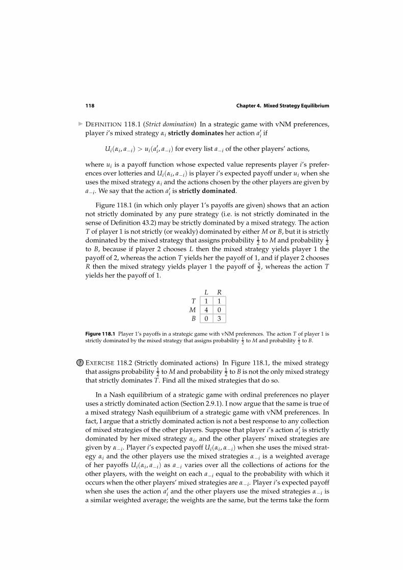
Figure 118.1 (in which only player 1’s payoffs are given) shows that an actionnot strictly dominated by any pure strategy (i.e. is not strictly dominated in thesense of Definition 43.2) may be strictly dominated by a mixed strategy. The actionT of player 1 is not strictly (or weakly) dominated by either M or B, but it is strictlydominated by the mixed strategy that assigns probability 1
2 to M and probability 12
to B, because if player 2 chooses L then the mixed strategy yields player 1 thepayoff of 2, whereas the action T yields her the payoff of 1, and if player 2 choosesR then the mixed strategy yields player 1 the payoff of 3
2 , whereas the action T
yields her the payoff of 1.
L R
T 1 1M 4 0B 0 3
Figure 118.1 Player 1’s payoffs in a strategic game with vNM preferences. The action T of player 1 isstrictly dominated by the mixed strategy that assigns probability 1
2 to M and probability 12 to B.
? EXERCISE 118.2 (Strictly dominated actions) In Figure 118.1, the mixed strategythat assigns probability 1
2 to M and probability 12 to B is not the only mixed strategy
that strictly dominates T. Find all the mixed strategies that do so.
In a Nash equilibrium of a strategic game with ordinal preferences no playeruses a strictly dominated action (Section 2.9.1). I now argue that the same is true ofa mixed strategy Nash equilibrium of a strategic game with vNM preferences. Infact, I argue that a strictly dominated action is not a best response to any collectionof mixed strategies of the other players. Suppose that player i’s action a′i is strictlydominated by her mixed strategy αi, and the other players’ mixed strategies aregiven by α−i. Player i’s expected payoff Ui(αi, α−i) when she uses the mixed strat-egy αi and the other players use the mixed strategies α−i is a weighted averageof her payoffs Ui(αi, a−i) as a−i varies over all the collections of actions for theother players, with the weight on each a−i equal to the probability with which itoccurs when the other players’ mixed strategies are α−i. Player i’s expected payoffwhen she uses the action a′i and the other players use the mixed strategies α−i isa similar weighted average; the weights are the same, but the terms take the form

4.4 Dominated actions 119
ui(a′i, a−i) rather than Ui(αi, a−i). The fact that a′i is strictly dominated by αi meansthat Ui(αi, a−i) > ui(a′i, a−i) for every collection a−i of the other players’ actions.Hence player i’s expected payoff when she uses the mixed strategy αi exceeds herexpected payoff when she uses the action a′i, given α−i. Consequently,
a strictly dominated action is not used with positive probability in any mixed
strategy equilibrium.
Thus when looking for mixed strategy equilibria we can eliminate from consider-ation every strictly dominated action.
As before, we can define the notion of weak domination (see Definition 45.1).
I DEFINITION 119.1 (Weak domination) In a strategic game with vNM preferences,player i’s mixed strategy αi weakly dominates her action a′i if
Ui(αi, a−i) ≥ ui(a′i, a−i) for every list a−i of the other players’ actions
and
Ui(αi, a−i) > ui(a′i, a−i) for some list a−i of the other players’ actions,
where ui is a payoff function whose expected value represents player i’s prefer-ences over lotteries and Ui(αi, a−i) is player i’s expected payoff under ui when sheuses the mixed strategy αi and the actions chosen by the other players are given bya−i. We say that the action a′i is weakly dominated.
We saw that a weakly dominated action may be used in a Nash equilibrium(see Figure 46.1). Thus a weakly dominated action may be used with positiveprobability in a mixed strategy equilibrium, so that we cannot eliminate weakly
dominated actions from consideration when finding mixed strategy equilibria!
? EXERCISE 119.2 (Eliminating dominated actions when finding equilibria) Find allthe mixed strategy Nash equilibria of the game in Figure 119.1 by first eliminatingany strictly dominated actions and then constructing the players’ best responsefunctions.
L M R
T 2, 2 0, 3 1, 2B 3, 1 1, 0 0, 2
Figure 119.1 The strategic game with vNM preferences in Exercise 119.2.
The fact that a player’s strategy in a mixed strategy Nash equilibrium may beweakly dominated raises the question of whether a game necessarily has a mixedstrategy Nash equilibrium in which no player’s strategy is weakly dominated. Thefollowing result (which is not easy to prove) shows that the answer is affirmativefor a finite game.

120 Chapter 4. Mixed Strategy Equilibrium
PROPOSITION 120.1 (Existence of mixed strategy Nash equilibrium with no weaklydominated strategies in finite games) Every strategic game with vNM preferences in
which each player has finitely many actions has a mixed strategy Nash equilibrium in
which no player’s strategy is weakly dominated.
4.5 Pure equilibria when randomization is allowed
The analysis in Section 4.3.6 shows that the mixed strategy Nash equilibria of BoS
in which each player’s strategy is pure correspond precisely to the Nash equilibriaof the version of the game (considered in Section 2.3) in which the players are notallowed to randomize. The same is true for a general game: equilibria when theplayers are not allowed to randomize remain equilibria when they are allowed torandomize, and any pure equilibria that exist when they are allowed to randomizeare equilibria when they are not allowed to randomize.
To establish this claim, let N be a set of players and let Ai, for each player i, bea set of actions. Consider the following two games.
G: the strategic game with ordinal preferences in which the set of players is N,the set of actions of each player i is Ai, and the preferences of each player i
are represented by the payoff function ui
G′: the strategic game with vNM preferences in which the set of players is N, theset of actions of each player i is Ai, and the preferences of each player i arerepresented by the expected value of ui.
First I argue that any Nash equilibrium of G corresponds to a mixed strategyNash equilibrium (in which each player’s strategy is pure) of G′. Let a∗ be a Nashequilibrium of G, and for each player i let α∗
i be the mixed strategy that assignsprobability 1 to a∗i . Since a∗ is a Nash equilibrium of G we know that in G′ noplayer i has an action that yields her a payoff higher than does a∗i when all the otherplayers adhere to α∗
−i. Thus α∗ satisfies the two conditions in Proposition 114.1, sothat it is a mixed strategy equilibrium of G′, establishing the following result.
PROPOSITION 120.2 (Pure strategy equilibria survive when randomization is al-lowed) Let a∗ be a Nash equilibrium of G and for each player i let α∗
i be the mixed strategy
of player i that assigns probability one to the action a∗i . Then α∗ is a mixed strategy Nash
equilibrium of G′.
Next I argue that any mixed strategy Nash equilibrium of G′ in which eachplayer’s strategy is pure corresponds to a Nash equilibrium of G. Let α∗ be a mixedstrategy Nash equilibrium of G′ in which every player’s mixed strategy is pure; foreach player i, denote by a∗i the action to which αi assigns probability one. Then nomixed strategy of player i yields her a payoff higher than does α∗
i when the otherplayers’ mixed strategies are given by α∗
−i. Hence, in particular, no pure strategyof player i yields her a payoff higher than does α∗
i . Thus a∗ is a Nash equilibriumof G. In words, if a pure strategy is optimal for a player when she is allowed
4.6 Illustration: expert diagnosis 121
to randomize then it remains optimal when she is prohibited from randomizing.(More generally, prohibiting a decision-maker from taking an action that is notoptimal does not change the set of actions that are optimal.)
PROPOSITION 121.1 (Pure strategy equilibria survive when randomization is pro-hibited) Let α∗ be a mixed strategy Nash equilibrium of G′ in which the mixed strategy of
each player i assigns probability one to the single action a∗i . Then a∗ is a Nash equilibrium
of G.
4.6 Illustration: expert diagnosis
I seem to confront the following predicament all too frequently. Something aboutwhich I am relatively ill-informed (my car, my computer, my body) stops workingproperly. I consult an expert, who makes a diagnosis and recommends an action.I am not sure if the diagnosis is correct—the expert, after all, has an interest inselling her services. I have to decide whether to follow the expert’s advice or to tryto fix the problem myself, put up with it, or consult another expert.
4.6.1 Model
A simple model that captures the main features of this situation starts with the as-sumption that there are two types of problem, major and minor. Denote the fractionof problems that are major by r, and assume that 0 < r < 1. An expert knows, onseeing a problem, whether it is major or minor; a consumer knows only the prob-ability r. (The diagnosis is costly neither to the expert nor to the consumer.) Anexpert may recommend either a major or a minor repair (regardless of the truenature of the problem), and a consumer may either accept the expert’s recommen-dation or seek another remedy. A major repair fixes both a major problem and aminor one.
Assume that a consumer always accepts an expert’s advice to obtain a minorrepair—there is no reason for her to doubt such a diagnosis—but may either ac-cept or reject advice to obtain a major repair. Further assume that an expert alwaysrecommends a major repair for a major problem—a minor repair does not fix amajor problem, so there is no point in an expert’s recommending one for a majorproblem—but may recommend either repair for a minor problem. Suppose that anexpert obtains the same profit π > 0 (per unit of time) from selling a minor repairto a consumer with a minor problem as she does from selling a major repair to aconsumer with a major problem, but obtains the profit π ′ > π from selling a majorrepair to a consumer with a minor problem. (The rationale is that in the last casethe expert does not in fact perform a major repair, at least not in its entirety.) Aconsumer pays an expert E for a major repair and I < E for a minor one; the costshe effectively bears if she chooses some other remedy is E′ > E if her problemis major and I ′ > I if it is minor. (Perhaps she consults other experts before pro-ceeding, or works on the problem herself, in either case spending valuable time.) Iassume throughout that E > I ′.

122 Chapter 4. Mixed Strategy Equilibrium
Under these assumptions we can model the situation as a strategic game inwhich the expert has two actions (recommend a minor repair for a minor problem;recommend a major repair for a minor problem), and the consumer has two ac-tions (accept the recommendation of a major repair; reject the recommendation ofa major repair). I name the actions as follows.
Expert Honest (recommend a minor repair for a minor problem and a major repairfor a major problem) and Dishonest (recommend a major repair for both typesof problem).
Consumer Accept (buy whatever repair the expert recommends) and Reject (buya minor repair but seek some other remedy if a major repair is recommended)
Assume that each player’s preferences are represented by her expected mone-tary payoff. Then the players’ payoffs to the four action pairs are as follows; thestrategic game is given in Figure 122.1.
(H, A): With probability r the consumer’s problem is major, so she pays E, andwith probability 1 − r it is minor, so she pays I. Thus her expected payoff is−rE − (1 − r)I. The expert’s profit is π.
(D, A): The consumer’s payoff is −E. The consumer’s problem is major withprobability r, yielding the expert π, and minor with probability 1 − r, yield-ing the expert π′, so that the expert’s expected payoff is rπ + (1 − r)π ′.
(H, R): The consumer’s cost is E′ if her problem is major (in which case she rejectsthe expert’s advice to get a major repair) and I if her problem is minor, so thather expected payoff is −rE′ − (1 − r)I. The expert obtains a payoff only if theconsumer’s problem is minor, in which case she gets π; thus her expectedpayoff is (1 − r)π.
(D, R): The consumer never accepts the expert’s advice, and thus obtains the ex-pected payoff −rE′ − (1 − r)I ′. The expert does not get any business, andthus obtains the payoff of 0.
Expert
ConsumerAccept (q) Reject (1 − q)
Honest (p) π, −rE − (1 − r)I (1 − r)π, −rE′ − (1 − r)I
Dishonest (1 − p) rπ + (1 − r)π′ , −E 0, −rE′ − (1 − r)I ′
Figure 122.1 A game between an expert and a consumer with a problem.
4.6.2 Nash equilibrium
To find the Nash equilibria of the game we can construct the best response func-tions, as before. Denote by p the probability the expert assigns to H and by q theprobability the consumer assigns to A.

4.6 Illustration: expert diagnosis 123
Expert’s best response function If q = 0 (i.e. the consumer chooses R with proba-bility one) then the expert’s best response is p = 1 (since (1 − r)π > 0). If q = 1(i.e. the consumer chooses A with probability one) then the expert’s best responseis p = 0 (since π′ > π, so that rπ + (1 − r)π′ > π). For what value of q is theexpert indifferent between H and D? Given q, the expert’s expected payoff to H
is qπ + (1 − q)(1 − r)π and her expected payoff to D is q[rπ + (1 − r)π ′ ], so she isindifferent between the two actions if
qπ + (1 − q)(1 − r)π = q[rπ + (1 − r)π ′ ].
Upon simplification, this yields q = π/π′. We conclude that the expert’s bestresponse function takes the form shown in both panels of Figure 124.1.
Consumer’s best response function If p = 0 (i.e. the expert chooses D with probabil-ity one) then the consumer’s best response depends on the relative sizes of E andrE′ + (1 − r)I ′. If E < rE′ + (1 − r)I ′ then the consumer’s best response is q = 1,whereas if E > rE′ + (1 − r)I ′ then her best response is q = 0; if E = rE′ + (1 − r)I ′
then she is indifferent between R and A.If p = 1 (i.e. the expert chooses H with probability one) then the consumer’s
best response is q = 1 (given E < E′).We conclude that if E < rE′ + (1 − r)I ′ then the consumer’s best response to
every value of p is q = 1, as shown in the left panel of Figure 124.1. If E > rE′ +(1 − r)I ′ then the consumer is indifferent between A and R if
p[rE + (1 − r)I] + (1 − p)E = p[rE′ + (1 − r)I] + (1 − p)[rE′ + (1 − r)I ′ ],
which reduces to
p =E − [rE′ + (1 − r)I ′ ]
(1 − r)(E − I ′).
In this case the consumer’s best response function takes the form shown in theright panel of Figure 124.1.
Equilibrium Given the best response functions, if E < rE′ + (1 − r)I ′ then the pairof pure strategies (D, A) is the unique Nash equilibrium. The condition E < rE′ +(1 − r)I ′ says that the cost of a major repair by an expert is less than the expected
cost of an alternative remedy; the only equilibrium yields the dismal outcome forthe consumer in which the expert is always dishonest and the consumer alwaysaccepts her advice.
If E > rE′ + (1 − r)I ′ then the unique equilibrium of the game is in mixedstrategies, with (p, q) = (p∗, q∗), where
p∗ =E − [rE′ + (1 − r)I ′ ]
(1 − r)(E − I ′)and q∗ =
π
π′ .
In this equilibrium the expert is sometimes honest, sometimes dishonest, and theconsumer sometimes accepts her advice to obtain a major repair, and sometimesignores such advice.

124 Chapter 4. Mixed Strategy Equilibrium
0 1p →
π/π′
1↑q
Expert
Consumer
E < rE′ + (1 − r)I ′
0 E−[rE′+(1−r)I′](1−r)(E−I′)
1p →
π/π′
1↑q
Expert
Consumer
E > rE′ + (1 − r)I ′
Figure 124.1 The players’ best response functions in the game of expert diagnosis. The probabilityassigned by the expert to H is p and the probability assigned by the consumer to A is q.
As discussed in the introduction to the chapter, a mixed strategy equilibriumcan be given more than one interpretation as a steady state. In the game we arestudying, and the games studied earlier in the chapter, I have focused on the in-terpretation in which each player chooses her action randomly, with probabilitiesgiven by her equilibrium mixed strategy, every time she plays the game. In thegame of expert diagnosis a different interpretation fits well: among the popula-tion of individuals who may play the role of each given player, every individualchooses the same action whenever she plays the game, but different individualschoose different actions; the fraction of individuals who choose each action is equalto the equilibrium probability that that action is used in a mixed strategy equilib-rium. Specifically, if E > rE′ + (1 − r)I ′ then the fraction p∗ of experts is honest(recommending minor repairs for minor problems) and the fraction 1 − p∗ is dis-honest (recommending major repairs for minor problems), while the fraction q∗ ofconsumers is credulous (accepting any recommendation) and the fraction 1 − q∗ iswary (accepting only a recommendation of a minor repair). Honest and dishonestexperts obtain the same expected payoff, as do credulous and wary consumers.
? EXERCISE 124.1 (Equilibrium in the expert diagnosis game) Find the set of mixedstrategy Nash equilibria of the game when E = rE′ + (1 − r)I ′.
4.6.3 Properties of the mixed strategy Nash equilibrium
Studying how the equilibrium is affected by changes in the parameters of themodel helps us understand the nature of the strategic interaction between theplayers. I consider the effects of three changes.
Suppose that major problems become less common (cars become more reli-able, more resources are devoted to preventive healthcare). If we rearrange the

4.6 Illustration: expert diagnosis 125
expression for p∗ to
p∗ = 1 − r(E′ − E)
(1 − r)(E − I ′),
we see that p∗ increases as r decreases (the numerator of the fraction decreases andthe denominator increases). Thus in a mixed strategy equilibrium, the experts aremore honest when major problems are less common. Intuitively, if a major prob-lem is less likely then a consumer has less to lose from ignoring an expert’s advice,so that the probability of an expert’s being honest has to rise in order that her ad-vice be heeded. The value of q∗ is not affected by the change in r: the probabilityof a consumer’s accepting an expert’s advice remains the same when major prob-lems become less common. Given the expert’s behavior, a decrease in r increasesthe consumer’s payoff to rejecting the expert’s advice more than it increases herpayoff to accepting this advice, so that she prefers to reject the advice. But thispartial analysis is misleading: in the equilibrium that exists after r decreases, theconsumer is exactly as likely to accept the expert’s advice as she was before thechange.
Now suppose that major repairs become less expensive relative to minor ones(technological advances reduce the cost of complex equipment). We see that p∗
decreases as E decreases (with E′ and I ′ constant): when major repairs are lesscostly, experts are less honest. As major repairs become less costly, a consumer hasmore potentially to lose from ignoring an expert’s advice, so that she heeds theadvice even if experts are less likely to be honest.
Finally, suppose that the profit π′ from an expert’s fixing a minor problem withan alleged major repair falls (the government requires experts to return replacedparts to the consumer, making it more difficult for an expert to fraudulently claimto have performed a major repair). Then q∗ increases—consumers become lesswary. Experts have less to gain from acting dishonestly, so that consumers can bemore confident of their advice.
? EXERCISE 125.1 (Incompetent experts) Consider a (realistic?) variant of the model,in which the experts are not entirely competent. Assume that each expert alwayscorrectly recognizes a major problem but correctly recognizes a minor problemwith probability s < 1: with probability 1 − s she mistakenly thinks that a minorproblem is major, and, if the consumer accepts her advice, performs a major repairand obtains the profit π. Maintain the assumption that each consumer believes(correctly) that the probability her problem is major is r. As before, a consumerwho does not give the job of fixing her problem to an expert bears the cost E′ if itis major and I ′ if it is minor.
Suppose, for example, that an expert is honest and a consumer rejects advice toobtain a major repair. With probability r the consumer’s problem is major, so thatthe expert recommends a major repair, which the consumer rejects; the consumerbears the cost E′. With probability 1 − r the consumer’s problem is minor. In thiscase with probability s the expert correctly diagnoses it as minor, and the consumeraccepts her advice and pays I; with probability 1 − s the expert diagnoses it as ma-

126 Chapter 4. Mixed Strategy Equilibrium
jor, and the consumer rejects her advice and bears the cost I ′. Thus the consumer’sexpected payoff in this case is −rE′ − (1 − r)[sI + (1 − s)I ′ ].
Construct the payoffs for every pair of actions and find the mixed strategy equi-librium in the case E > rE′ + (1− r)I ′. Does incompetence breed dishonesty? Morewary consumers?
? EXERCISE 126.1 (Choosing a seller) Each of two sellers has available one indivisibleunit of a good. Seller 1 posts the price p1 and seller 2 posts the price p2. Each oftwo buyers would like to obtain one unit of the good; they simultaneously decidewhich seller to approach. If both buyers approach the same seller, each trades withprobability 1
2 ; the disappointed buyer does not subsequently have the option totrade with the other seller. (This assumption models the risk faced by a buyer thata good is sold out when she patronizes a seller with a low price.) Each buyer’spreferences are represented by the expected value of a payoff function that assignsthe payoff 0 to not trading and the payoff 1 − p to purchasing one unit of the goodat the price p. (Neither buyer values more than one unit.) For any pair (p1, p2) ofprices with 0 ≤ pi ≤ 1 for i = 1, 2, find the Nash equilibria (in pure and in mixedstrategies) of the strategic game that models this situation. (There are three maincases: p2 < 2p1 − 1, 2p1 − 1 < p2 < 1
2 (1 + p1), and p2 > 12 (1 + p1).)
4.7 Equilibrium in a single population
In Section 2.10 I discussed deterministic steady states in situations in which themembers of a single population interact. I now discuss stochastic steady states insuch situations.
First extend the definitions of a symmetric strategic game and a symmetricNash equilibrium (Definitions 49.3 and 50.2) to a game with vNM preferences. Re-call that a two-player strategic game with ordinal preferences is symmetric if eachplayer has the same set of actions and each player’s evaluation of an outcome de-pends only on her action and that of her opponent, not on whether she is player 1or player 2. A symmetric game with vNM preferences satisfies the same condi-tions; its definition differs from Definition 49.3 only because a player’s evaluationof an outcome is given by her expected payoff rather than her ordinal preferences.
I DEFINITION 126.2 (Symmetric two-player strategic game with vNM preferences) Atwo-player strategic game with vNM preferences is symmetric if the players’ setsof actions are the same and the players’ preferences are represented by the ex-pected values of payoff functions u1 and u2 for which u1(a1, a2) = u2(a2, a1) forevery action pair (a1, a2).
A Nash equilibrium of a strategic game with ordinal preferences in which ev-ery player’s set of actions is the same is symmetric if all players take the sameaction. This notion of equilibrium extends naturally to strategic games with vNMpreferences. (As before, it does not depend on the game’s having only two players,so I define it for a game with any number of players.)

4.7 Equilibrium in a single population 127
I DEFINITION 127.1 (Symmetric mixed strategy Nash equilibrium) A profile α∗ of mixedstrategies in a strategic game with vNM preferences in which each player has thesame set of actions is a symmetric mixed strategy Nash equilibrium if it is a mixedstrategy Nash equilibrium and α∗
i is the same for every player i.
Now consider again the game of approaching pedestrians (Figure 51.1, repro-duced in Figure 127.1), interpreting the payoff numbers as Bernoulli payoffs whoseexpected values represent the players’ preferences over lotteries. We found thatthis game has two deterministic steady states, corresponding to the two symmet-ric Nash equilibria in pure strategies, (Left, Left) and (Right, Right). The game alsohas a symmetric mixed strategy Nash equilibrium, in which each player assignsprobability 1
2 to Left and probability 12 to Right. This equilibrium corresponds to a
steady state in which half of all encounters result in collisions! (With probability 14
player 1 chooses Left and player 2 chooses Right, and with probability 14 player 1
chooses Right and player 2 chooses Left.)
Left Right
Left 1, 1 0, 0Right 0, 0 1, 1
Figure 127.1 Approaching pedestrians.
In this example not only is the game symmetric, but the players’ interests coin-cide. The game in Figure 127.2 is symmetric, but the players prefer to take differ-ent actions rather than the same actions. This game has no pure symmetric equi-librium, but has a symmetric mixed strategy equilibrium, in which each playerchooses each action with probability 1
2 .
X Y
X 0, 0 1, 1Y 1, 1 0, 0
Figure 127.2 A symmetric game.
These two examples show that a symmetric game may have no symmetric pure
strategy equilibrium. But both games have a symmetric mixed strategy Nash equi-librium, as does any symmetric game in which each player has finitely many ac-tions, by the following result. (Relatively advanced mathematical tools are neededto prove the result.)
PROPOSITION 127.2 (Existence of symmetric mixed strategy Nash equilibrium insymmetric finite games) Every strategic game with vNM preferences in which each
player has the same finite set of actions has a symmetric mixed strategy Nash equilibrium.
? EXERCISE 127.3 (Approaching cars) Members of a single population of car driversare randomly matched in pairs when they simultaneously approach intersections
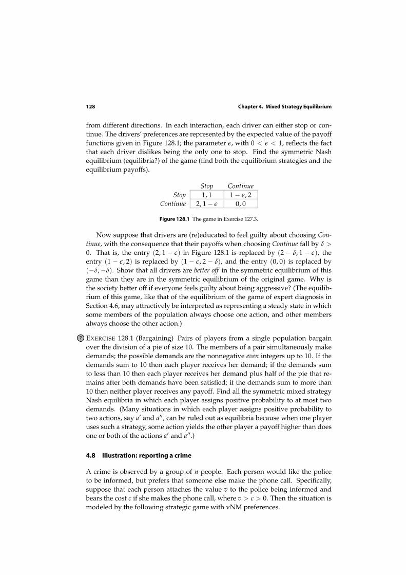
128 Chapter 4. Mixed Strategy Equilibrium
from different directions. In each interaction, each driver can either stop or con-tinue. The drivers’ preferences are represented by the expected value of the payofffunctions given in Figure 128.1; the parameter ε, with 0 < ε < 1, reflects the factthat each driver dislikes being the only one to stop. Find the symmetric Nashequilibrium (equilibria?) of the game (find both the equilibrium strategies and theequilibrium payoffs).
Stop Continue
Stop 1, 1 1 − ε, 2Continue 2, 1 − ε 0, 0
Figure 128.1 The game in Exercise 127.3.
Now suppose that drivers are (re)educated to feel guilty about choosing Con-
tinue, with the consequence that their payoffs when choosing Continue fall by δ >
0. That is, the entry (2, 1 − ε) in Figure 128.1 is replaced by (2 − δ, 1 − ε), theentry (1 − ε, 2) is replaced by (1 − ε, 2 − δ), and the entry (0, 0) is replaced by(−δ, −δ). Show that all drivers are better off in the symmetric equilibrium of thisgame than they are in the symmetric equilibrium of the original game. Why isthe society better off if everyone feels guilty about being aggressive? (The equilib-rium of this game, like that of the equilibrium of the game of expert diagnosis inSection 4.6, may attractively be interpreted as representing a steady state in whichsome members of the population always choose one action, and other membersalways choose the other action.)
? EXERCISE 128.1 (Bargaining) Pairs of players from a single population bargainover the division of a pie of size 10. The members of a pair simultaneously makedemands; the possible demands are the nonnegative even integers up to 10. If thedemands sum to 10 then each player receives her demand; if the demands sumto less than 10 then each player receives her demand plus half of the pie that re-mains after both demands have been satisfied; if the demands sum to more than10 then neither player receives any payoff. Find all the symmetric mixed strategyNash equilibria in which each player assigns positive probability to at most twodemands. (Many situations in which each player assigns positive probability totwo actions, say a′ and a′′, can be ruled out as equilibria because when one playeruses such a strategy, some action yields the other player a payoff higher than doesone or both of the actions a′ and a′′.)
4.8 Illustration: reporting a crime
A crime is observed by a group of n people. Each person would like the policeto be informed, but prefers that someone else make the phone call. Specifically,suppose that each person attaches the value v to the police being informed andbears the cost c if she makes the phone call, where v > c > 0. Then the situation ismodeled by the following strategic game with vNM preferences.
4.8 Illustration: reporting a crime 129
Players The n people.
Actions Each player’s set of actions is {Call, Don’t call}.
Preferences Each player’s preferences are represented by the expected value ofa payoff function that assigns 0 to the profile in which no one calls, v − c
to any profile in which she calls, and v to any profile in which at least oneperson calls, but she does not.
This game is a variant of the one in Exercise 31.1, with k = 1. It has n pure Nashequilibria, in each of which exactly one person calls. (If that person switches to notcalling, her payoff falls from v − c to 0; if any other person switches to calling, herpayoff falls from v to v− c.) If the members of the group differ in some respect, thenthese asymmetric equilibria may be compelling as steady states. For example, thesocial norm in which the oldest person in the group makes the phone call is stable.
If the members of the group either do not differ significantly or are not awareof any differences among themselves—if they are drawn from a single homoge-neous population—then there is no way for them to coordinate, and a symmetricequilibrium, in which every player uses the same strategy, is more compelling.
The game has no symmetric pure Nash equilibrium. (If everyone calls, thenany person is better off switching to not calling. If no one calls, then any person isbetter off switching to calling.)
However, it has a symmetric mixed strategy equilibrium in which each personcalls with positive probability less than one. In any such equilibrium, each per-son’s expected payoff to calling is equal to her expected payoff to not calling. Eachperson’s payoff to calling is v − c, and her payoff to not calling is 0 if no one elsecalls and v if at least one other person calls, so the equilibrium condition is
v − c = 0 · Pr{no one else calls} + v · Pr{at least one other person calls},
orv − c = v · (1 − Pr{no one else calls}),
orc/v = Pr{no one else calls}. (129.1)
Denote by p the probability with which each person calls. The probability thatno one else calls is the probability that every one of the other n − 1 people does notcall, namely (1 − p)n−1. Thus the equilibrium condition is c/v = (1 − p)n−1, or
p = 1 − (c/v)1/(n−1).
This number p is between 0 and 1, so we conclude that the game has a uniquesymmetric mixed strategy equilibrium, in which each person calls with probability1 − (c/v)1/(n−1). That is, there is a steady state in which whenever a person isin a group of n people facing the situation modeled by the game, she calls withprobability 1 − (c/v)1/(n−1).
130 Chapter 4. Mixed Strategy Equilibrium
How does this equilibrium change as the size of the group increases? We seethat as n increases, the probability p that any given person calls decreases. (Asn increases, 1/(n − 1) decreases, so that (c/v)1/(n−1) increases.) What about theprobability that at least one person calls? Fix any player i. Then the event “no onecalls” is the same as the event “i does not call and no one other than i calls”. Thus
Pr{no one calls} = Pr{i does not call} · Pr{no one else calls}. (130.1)
Now, the probability that any given person calls decreases as n increases, or equiv-alently the probability that she does not call increases as n increases. Further, fromthe equilibrium condition (129.1), Pr{no one else calls} is equal to c/v, independent
of n. We conclude that the probability that no one calls increases as n increases.That is, the larger the group, the less likely the police are informed of the crime!
The condition defining a mixed strategy equilibrium is responsible for this re-sult. For any given person to be indifferent between calling and not calling thiscondition requires that the probability that no one else calls be independent of thesize of the group. Thus each person’s probability of not calling is larger in a largergroup, and hence, by the laws of probability reflected in (130.1), the probabilitythat no one calls is larger in a larger group.
The result that the larger the group, the less likely any given person calls is notsurprising. The result that the larger the group, the less likely at least one personcalls is a more subtle implication of the notion of equilibrium. In a larger group noindividual is any less concerned that the police should be called, but in a steadystate the behavior of the group drives down the chance that the police are notifiedof the crime.
? EXERCISE 130.2 (Reporting a crime when the witnesses are heterogeneous) Con-sider a variant of the model studied in this section in which n1 witnesses incur thecost c1 to report the crime, and n2 witnesses incur the cost c2, where 0 < c1 < v,0 < c2 < v, and n1 + n2 = n. Show that if c1 and c2 are sufficiently close the gamehas a mixed strategy Nash equilibrium in which every witness’s strategy assignspositive probabilities to both reporting and not reporting.
? EXERCISE 130.3 (Contributing to a public good) Consider an extension of the anal-ysis above to the game in Exercise 31.1 for k ≥ 2. (In this case a player may con-tribute even though the good is not provided; the player’s payoff in this case is −c.)Denote by Qn−1,m(p) the probability that exactly m of a group of n − 1 players con-tribute when each player contributes with probability p. What condition must besatisfied by Qn−1,k−1(p) in a symmetric mixed strategy equilibrium (in which eachplayer contributes with the same probability)? (When does a player’s contributionmake a difference to the outcome?) For the case v = 1, n = 4, k = 2, and c = 3
8 findthe equilibria explicitly. (You need to use the fact that Q3,1(p) = 3p(1 − p)2, anddo a bit of algebra.)

4.8 Illustration: reporting a crime 131
REPORTING A CRIME: SOCIAL PSYCHOLOGY AND GAME THEORY
Thirty-eight people witnessed the brutal murder of Catherine (“Kitty”) Genoveseover a period of half an hour in New York City in March 1964. During this period,none of them significantly responded to her screams for help; none even called thepolice. Journalists, psychiatrists, sociologists, and others subsequently struggledto understand the witnesses’ inaction. Some ascribed it to apathy engendered bylife in a large city: “Indifference to one’s neighbor and his troubles is a conditionedreflex of life in New York as it is in other big cities” (Rosenthal 1964, 81–82).
The event particularly interested social psychologists. It led them to try to un-derstand the circumstances under which a bystander would help someone in trou-ble. Experiments quickly suggested that, contrary to the popular theory, people—even those living in large cities—are not in general apathetic to others’ plights. Anexperimental subject who is the lone witness of a person in distress is very likelyto try to help. But as the size of the group of witnesses increases, there is a declinenot only in the probability that any given one of them offers assistance, but alsoin the probability that at least one of them offers assistance. Social psychologistshypothesize that three factors explain these experimental findings. First, “diffu-sion of responsibility”: the larger the group, the lower the psychological cost ofnot helping. Second, “audience inhibition”: the larger the group, the greater theembarrassment suffered by a helper in case the event turns out to be one in whichhelp is inappropriate (because, for example, it is not in fact an emergency). Third,“social influence”: a person infers the appropriateness of helping from others’ be-havior, so that in a large group everyone else’s lack of intervention leads any givenperson to think intervention is less likely to be appropriate.
In terms of the model in Section 4.8, these three factors raise the expectedcost and/or reduce the expected benefit of a person’s intervening. They all seemplausible. However, they are not needed to explain the phenomenon: our game-theoretic analysis shows that even if the cost and benefit are independent of groupsize, a decrease in the probability that at least one person intervenes is an implica-tion of equilibrium. This game-theoretic analysis has an advantage over the socio-psychological one: it derives the conclusion from the same principles that underlieall the other models studied so far (oligopoly, auctions, voting, and elections, forexample), rather than positing special features of the specific environment in whicha group of bystanders may come to the aid of a person in distress.
The critical element missing from the socio-psychological analysis is the notionof an equilibrium. Whether any given person intervenes depends on the probabilityshe assigns to some other person’s intervening. In an equilibrium each personmust be indifferent between intervening and not intervening, and as we have seenthis condition leads inexorably to the conclusion that an increase in group sizereduces the probability that at least one person intervenes.

132 Chapter 4. Mixed Strategy Equilibrium
4.9 The formation of players’ beliefs
In a Nash equilibrium, each player chooses a strategy that maximizes her expectedpayoff, knowing the other players’ strategies. So far we have not considered howplayers may acquire such information. Informally, the idea underlying the pre-vious analysis is that the players have learned each other’s strategies from theirexperience playing the game. In the idealized situation to which the analysis cor-responds, for each player in the game there is a large population of individualswho may take the role of that player; in any play of the game, one participant isdrawn randomly from each population. In this situation, a new individual whojoins a population that is in a steady state (i.e. is using a Nash equilibrium strategyprofile) can learn the other players’ strategies by observing their actions over manyplays of the game. As long as the turnover in players is small enough, existingplayers’ encounters with neophytes (who may use nonequilibrium strategies) willbe sufficiently rare that their beliefs about the steady state will not be disturbed, sothat a new player’s problem is simply to learn the other players’ actions.
This analysis leaves open the question of what might happen if new playerssimultaneously join more than one population in sufficient numbers that they havea significant chance of facing opponents who are themselves new. In particular,can we expect a steady state to be reached when no one has experience playing thegame?
4.9.1 Eliminating dominated actions
In some games the players may reasonably be expected to choose their Nash equi-librium actions from an introspective analysis of the game. At an extreme, eachplayer’s best action may be independent of the other players’ actions, as in thePrisoner’s Dilemma (Example 12.1). In such a game no player needs to worry aboutthe other players’ actions. In a less extreme case, some player’s best action maydepend on the other players’ actions, but the actions the other players will choosemay be clear because each of these players has an action that strictly dominatesall others. For example, in the game in Figure 132.1, player 2’s action R strictlydominates L, so that no matter what player 2 thinks player 1 will do, she shouldchoose R. Consequently, player 1, who can deduce by this argument that player 2will choose R, may reason that she should choose B. That is, even inexperiencedplayers may be led to the unique Nash equilibrium (B, R) in this game.
L R
T 1, 2 0, 3B 0, 0 1, 1
Figure 132.1 A game in which player 2 has a strictly dominant action whereas player 1 does not.
This line of argument may be extended. For example, in the game in Fig-ure 133.1 player 1’s action T is strictly dominated, so player 1 may reason that
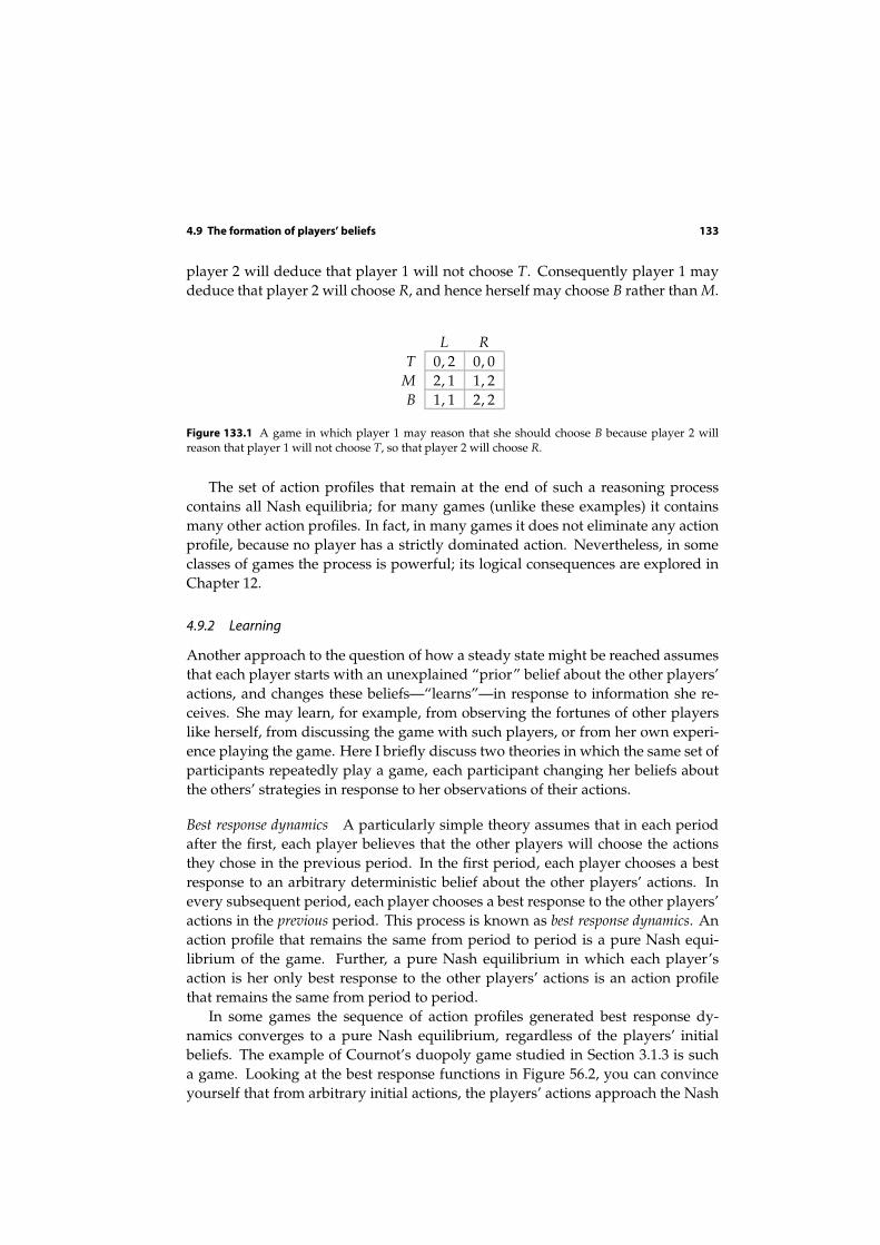
4.9 The formation of players’ beliefs 133
player 2 will deduce that player 1 will not choose T. Consequently player 1 maydeduce that player 2 will choose R, and hence herself may choose B rather than M.
L R
T 0, 2 0, 0M 2, 1 1, 2B 1, 1 2, 2
Figure 133.1 A game in which player 1 may reason that she should choose B because player 2 willreason that player 1 will not choose T, so that player 2 will choose R.
The set of action profiles that remain at the end of such a reasoning processcontains all Nash equilibria; for many games (unlike these examples) it containsmany other action profiles. In fact, in many games it does not eliminate any actionprofile, because no player has a strictly dominated action. Nevertheless, in someclasses of games the process is powerful; its logical consequences are explored inChapter 12.
4.9.2 Learning
Another approach to the question of how a steady state might be reached assumesthat each player starts with an unexplained “prior” belief about the other players’actions, and changes these beliefs—“learns”—in response to information she re-ceives. She may learn, for example, from observing the fortunes of other playerslike herself, from discussing the game with such players, or from her own experi-ence playing the game. Here I briefly discuss two theories in which the same set ofparticipants repeatedly play a game, each participant changing her beliefs aboutthe others’ strategies in response to her observations of their actions.
Best response dynamics A particularly simple theory assumes that in each periodafter the first, each player believes that the other players will choose the actionsthey chose in the previous period. In the first period, each player chooses a bestresponse to an arbitrary deterministic belief about the other players’ actions. Inevery subsequent period, each player chooses a best response to the other players’actions in the previous period. This process is known as best response dynamics. Anaction profile that remains the same from period to period is a pure Nash equi-librium of the game. Further, a pure Nash equilibrium in which each player’saction is her only best response to the other players’ actions is an action profilethat remains the same from period to period.
In some games the sequence of action profiles generated best response dy-namics converges to a pure Nash equilibrium, regardless of the players’ initialbeliefs. The example of Cournot’s duopoly game studied in Section 3.1.3 is sucha game. Looking at the best response functions in Figure 56.2, you can convinceyourself that from arbitrary initial actions, the players’ actions approach the Nash

134 Chapter 4. Mixed Strategy Equilibrium
equilibrium (q∗1, q∗2).
? EXERCISE 134.1 (Best response dynamics in Cournot’s duopoly game) Find thesequence of pairs of outputs chosen by the firms in Cournot’s duopoly game underthe assumptions of Section 3.1.3 if they both initially choose 0. (If you know howto solve a first-order difference equation, find a formula for the outputs in eachperiod; if not, find the outputs in the first few periods.)
? EXERCISE 134.2 (Best response dynamics in Bertrand’s duopoly game) ConsiderBertrand’s duopoly game in which the set of possible prices is discrete, under theassumptions of Exercise 65.2. Does the sequences of prices under best responsedynamics converge to a Nash equilibrium when both prices initially exceed c + 1?What happens when both prices are initially equal to c?
For other games there are initial beliefs for which the sequence of action profilesgenerated by the process does not converge. In BoS (Example 16.2), for example, ifplayer 1 initially believes that player 2 will choose Stravinsky and player 2 initiallybelieves that player 1 will choose Bach, then the players’ choices will subsequentlyalternate indefinitely between the action pairs (Bach, Stravinsky) and (Stravinsky, Bach).This example highlights the limited extent to which a player is assumed to reasonin the model, which does not consider the possibility that she cottons on to the factthat her opponent’s action is always a best response to her own previous action.
Fictitious play Under best response dynamics, the players’ beliefs are continuallyrevealed to be incorrect unless the starting point is a Nash equilibrium: the players’actions change from period to period. Further, each player believes that everyother player is using a pure strategy: a player’s belief does not admit the possibilitythat her opponents’ actions are realizations of mixed strategies.
Another theory, known as fictitious play, assumes that players consider actionsin all the previous periods when forming a belief about their opponents’ strategies.They treat these actions as realizations of mixed strategies. Consider a two-playergame. Each player begins with an arbitrary probabilistic belief about the otherplayer’s action. In the first play of the game she chooses a best response to thisbelief and observes the other player’s action, say A. She then changes her beliefto one that assigns probability one to A; in the second period, she chooses a bestresponse to this belief and observes the other player’s action, say B. She thenchanges her belief to one that assigns probability 1
2 to both A and B, and choosesa best response to this belief. She continues to change her belief each period; inany period she adopts the belief that her opponent is using a mixed strategy inwhich the probability of each action is proportional to the frequency with whichher opponent chose that action in the previous periods. (If, for example, in the firstsix periods player 2 chooses A twice, B three times, and C once, player 1’s belief inperiod 7 assigns probability 1
3 to A, probability 12 to B, and probability 1
6 to C.)In the game Matching Pennies (Example 17.1), reproduced in Figure 135.1, this
process works as follows. Suppose that player 1 begins with the belief that player 2’s

4.10 Extension: Finding all mixed strategy Nash equilibria 135
action will be Tail, and player 2 begins with the belief that player 1’s action willbe Head. Then in period 1 both players choose Tail. Thus in period 2 both play-ers believe that their opponent will choose Tail, so that player 1 chooses Tail andplayer 2 chooses Head. Consequently in period 3, player 1’s belief is that player 2will choose Head with probability 1
2 and Tail with probability 12 , and player 2’s be-
lief is that player 1 will definitely choose Tail. Thus in period 3, both Head andTail are best responses of player 1 to her belief, so that she may take either action;the unique best response of player 2 is Head. The process continues similarly insubsequent periods.
Head Tail
Head 1, −1 −1, 1Tail −1, 1 1, −1
Figure 135.1 Matching Pennies.
In two-player games like Matching Pennies, in which the players’ interests aredirectly opposed, and in any two-player game in which each player has two ac-tions, this process converges to a mixed strategy Nash equilibrium from any initialbeliefs. That is, after a sufficiently large number of periods, the frequencies withwhich each player chooses her actions are close to the frequencies induced by hermixed strategy in the Nash equilibrium. For other games there are initial beliefsfor which the process does not converge. (The simplest example is too complicatedto present compactly.)
People involved in an interaction that we model as a game may form beliefsabout their opponents’ strategies from an analysis of the structure of the players’payoffs, from their observations of their opponents’ actions, and from informationthey obtain from other people involved in similar interactions. The models I haveoutlined allow us to explore the logical implications of two ways in which play-ers may draw inferences from their opponents’ actions. Models that assume theplayers to be more sophisticated may give more insights into the types of situationin which a Nash equilibrium is likely to be attained; this topic is an active area ofcurrent research.
4.10 Extension: Finding all mixed strategy Nash equilibria
We can find all the mixed strategy Nash equilibria of a two-player game in whicheach player has two actions by constructing the players’ best response functions,as we have seen. In more complicated games, this method is usually not practical.
The following systematic method of finding all mixed strategy Nash equilib-ria of a game is suggested by the characterization of an equilibrium in Proposi-tion 114.1.
• For each player i, choose a subset Si of her set Ai of actions.

136 Chapter 4. Mixed Strategy Equilibrium
• Check whether there exists a mixed strategy profile α such that (i) the set ofactions to which each strategy αi assigns positive probability is Si and (ii) α
satisfies the conditions in Proposition 114.1.
• Repeat the analysis for every collection of subsets of the players’ sets ofactions.
The following example illustrates this method for a two-player game in whicheach player has two actions.
EXAMPLE 136.1 (Finding all mixed strategy equilibria of a two-player game inwhich each player has two actions) Consider a two-player game in which eachplayer has two actions. Denote the actions and payoffs as in Figure 137.1. Eachplayer’s set of actions has three nonempty subsets: two each consisting of a sin-gle action, and one consisting of both actions. Thus there are nine (3 × 3) pairs ofsubsets of the players’ action sets. For each pair (S1, S2), we check if there is a pair(α1, α2) of mixed strategies such that each strategy αi assigns positive probabilityonly to actions in Si and the conditions in Proposition 114.1 are satisfied.
• Checking the four pairs of subsets in which each player’s subset consists of asingle action amounts to checking whether any of the four pairs of actions isa pure strategy equilibrium. (For each player, the first condition in Proposi-tion 114.1 is automatically satisfied, because there is only one action in eachsubset.)
• Consider the pair of subsets {T, B} for player 1 and {L} for player 2. Thesecond condition in Proposition 114.1 is automatically satisfied for player 1,who has no actions to which she assigns probability 0, and the first conditionis automatically satisfied for player 2, because she assigns positive probabilityto only one action. Thus for there to be a mixed strategy equilibrium in whichplayer 1’s probability of using T is p we need u11 = u21 (player 1’s payoffs toher two actions must be equal) and
pv11 + (1 − p)v21 ≥ pv12 + (1 − p)v22
(L must be at least as good as R, given player 1’s mixed strategy). If u11 6=u21, or if there is no probability p satisfying the inequality, then there is noequilibrium of this type. A similar argument applies to the three other pairsof subsets in which one player’s subset consists of both her actions and theother player’s subset consists of a single action.
• To check whether there is a mixed strategy equilibrium in which the sub-sets are {T, B} for player 1 and {L, R} for player 2, we need to find a pair ofmixed strategies that satisfies the first condition in Proposition 114.1 (the sec-ond condition is automatically satisfied because both players assign positiveprobability to both their actions). That is, we need to find probabilities p andq (if any such exist) for which
qu11 + (1− q)u12 = qu21 + (1− q)u22 and pv11 + (1− p)v21 = pv12 + (1− p)v22.
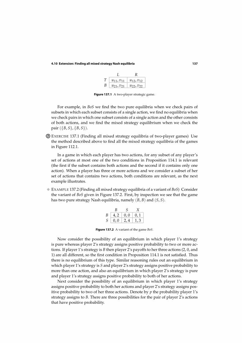
4.10 Extension: Finding all mixed strategy Nash equilibria 137
L R
T u11, v11 u12, v12B u21, v21 u22, v22
Figure 137.1 A two-player strategic game.
For example, in BoS we find the two pure equilibria when we check pairs ofsubsets in which each subset consists of a single action, we find no equilibria whenwe check pairs in which one subset consists of a single action and the other consistsof both actions, and we find the mixed strategy equilibrium when we check thepair ({B, S}, {B, S}).
? EXERCISE 137.1 (Finding all mixed strategy equilibria of two-player games) Usethe method described above to find all the mixed strategy equilibria of the gamesin Figure 112.1.
In a game in which each player has two actions, for any subset of any player’sset of actions at most one of the two conditions in Proposition 114.1 is relevant(the first if the subset contains both actions and the second if it contains only oneaction). When a player has three or more actions and we consider a subset of herset of actions that contains two actions, both conditions are relevant, as the nextexample illustrates.
EXAMPLE 137.2 (Finding all mixed strategy equilibria of a variant of BoS) Considerthe variant of BoS given in Figure 137.2. First, by inspection we see that the gamehas two pure strategy Nash equilibria, namely (B, B) and (S, S).
B S X
B 4, 2 0, 0 0, 1S 0, 0 2, 4 1, 3
Figure 137.2 A variant of the game BoS.
Now consider the possibility of an equilibrium in which player 1’s strategyis pure whereas player 2’s strategy assigns positive probability to two or more ac-tions. If player 1’s strategy is B then player 2’s payoffs to her three actions (2, 0, and1) are all different, so the first condition in Proposition 114.1 is not satisfied. Thusthere is no equilibrium of this type. Similar reasoning rules out an equilibrium inwhich player 1’s strategy is S and player 2’s strategy assigns positive probability tomore than one action, and also an equilibrium in which player 2’s strategy is pureand player 1’s strategy assigns positive probability to both of her actions.
Next consider the possibility of an equilibrium in which player 1’s strategyassigns positive probability to both her actions and player 2’s strategy assigns pos-itive probability to two of her three actions. Denote by p the probability player 1’sstrategy assigns to B. There are three possibilities for the pair of player 2’s actionsthat have positive probability.
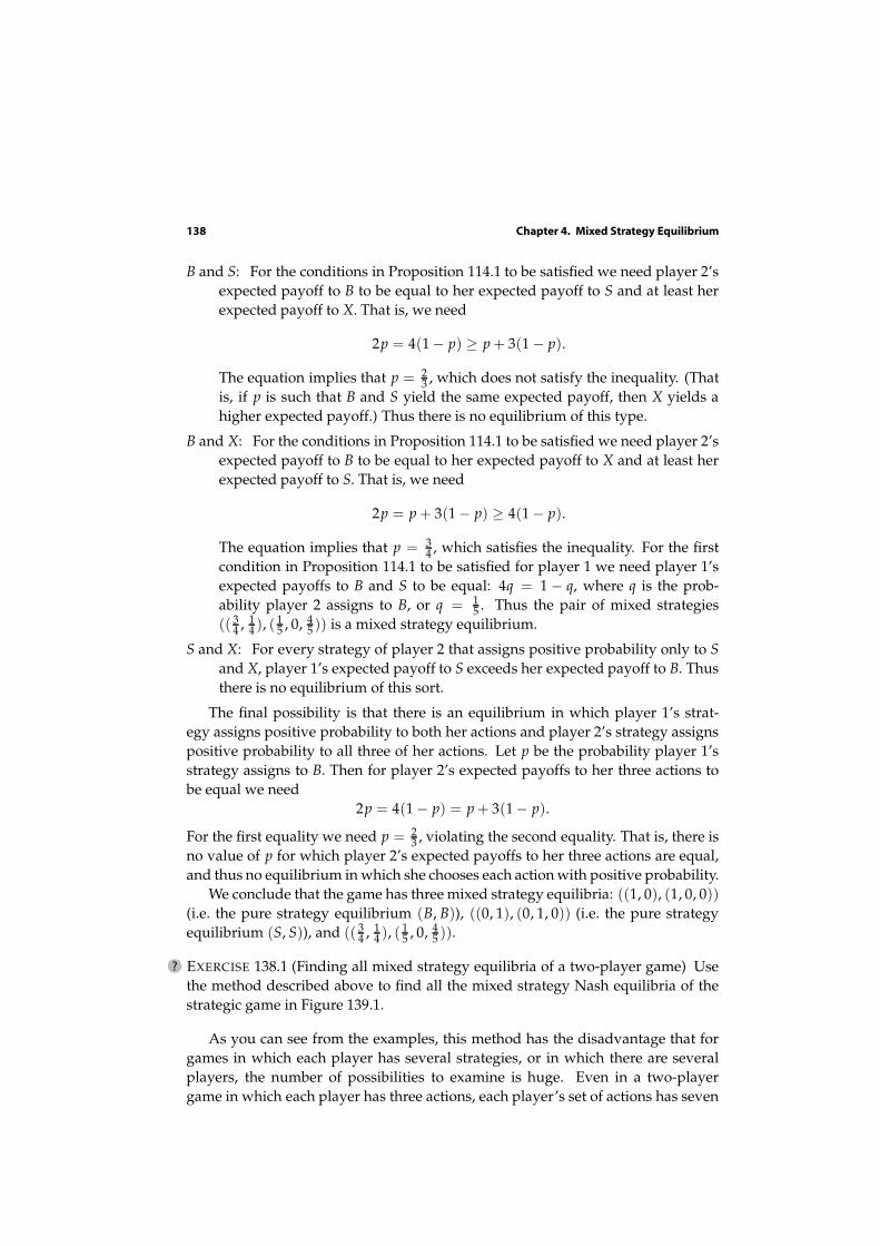
138 Chapter 4. Mixed Strategy Equilibrium
B and S: For the conditions in Proposition 114.1 to be satisfied we need player 2’sexpected payoff to B to be equal to her expected payoff to S and at least herexpected payoff to X. That is, we need
2p = 4(1 − p) ≥ p + 3(1 − p).
The equation implies that p = 23 , which does not satisfy the inequality. (That
is, if p is such that B and S yield the same expected payoff, then X yields ahigher expected payoff.) Thus there is no equilibrium of this type.
B and X: For the conditions in Proposition 114.1 to be satisfied we need player 2’sexpected payoff to B to be equal to her expected payoff to X and at least herexpected payoff to S. That is, we need
2p = p + 3(1 − p) ≥ 4(1 − p).
The equation implies that p = 34 , which satisfies the inequality. For the first
condition in Proposition 114.1 to be satisfied for player 1 we need player 1’sexpected payoffs to B and S to be equal: 4q = 1 − q, where q is the prob-ability player 2 assigns to B, or q = 1
5 . Thus the pair of mixed strategies(( 3
4 , 14 ), ( 1
5 , 0, 45 )) is a mixed strategy equilibrium.
S and X: For every strategy of player 2 that assigns positive probability only to S
and X, player 1’s expected payoff to S exceeds her expected payoff to B. Thusthere is no equilibrium of this sort.
The final possibility is that there is an equilibrium in which player 1’s strat-egy assigns positive probability to both her actions and player 2’s strategy assignspositive probability to all three of her actions. Let p be the probability player 1’sstrategy assigns to B. Then for player 2’s expected payoffs to her three actions tobe equal we need
2p = 4(1 − p) = p + 3(1 − p).
For the first equality we need p = 23 , violating the second equality. That is, there is
no value of p for which player 2’s expected payoffs to her three actions are equal,and thus no equilibrium in which she chooses each action with positive probability.
We conclude that the game has three mixed strategy equilibria: ((1, 0), (1, 0, 0))
(i.e. the pure strategy equilibrium (B, B)), ((0, 1), (0, 1, 0)) (i.e. the pure strategyequilibrium (S, S)), and (( 3
4 , 14 ), ( 1
5 , 0, 45 )).
? EXERCISE 138.1 (Finding all mixed strategy equilibria of a two-player game) Usethe method described above to find all the mixed strategy Nash equilibria of thestrategic game in Figure 139.1.
As you can see from the examples, this method has the disadvantage that forgames in which each player has several strategies, or in which there are severalplayers, the number of possibilities to examine is huge. Even in a two-playergame in which each player has three actions, each player’s set of actions has seven
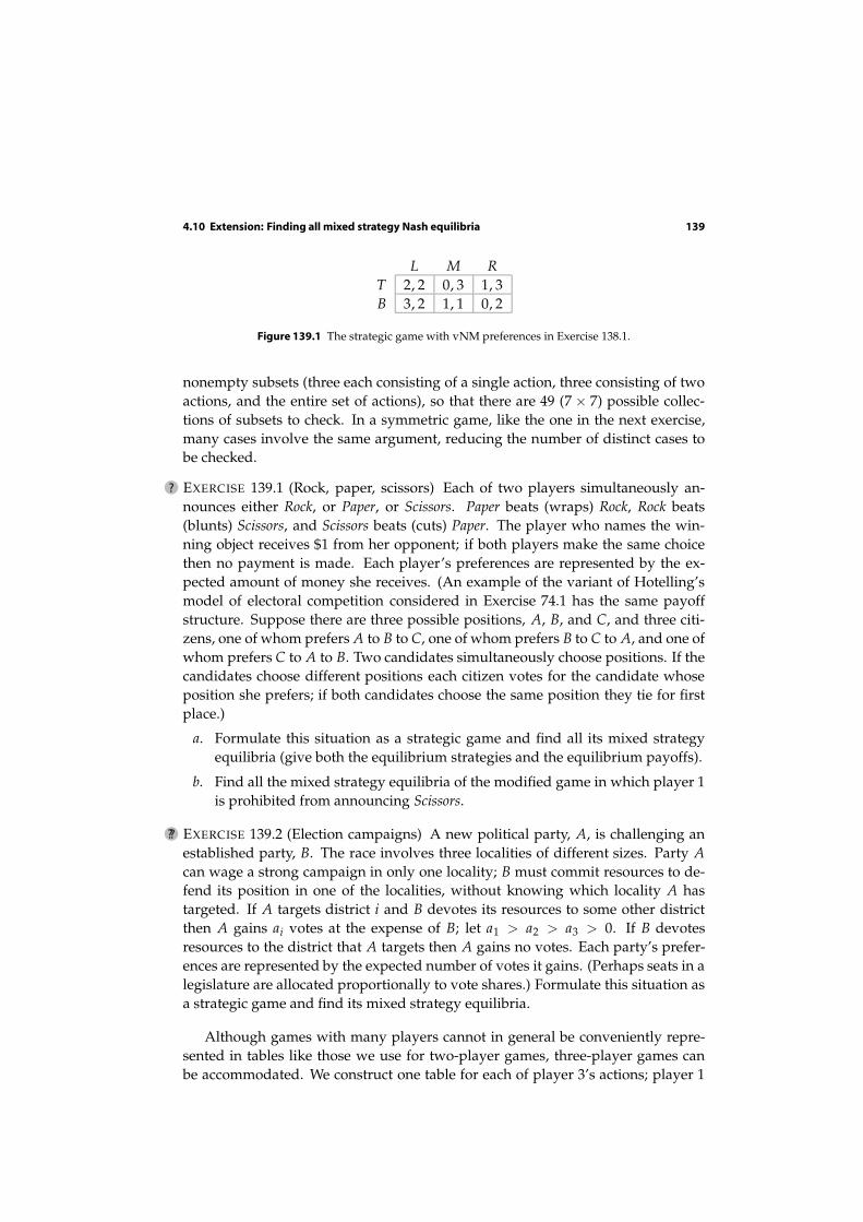
4.10 Extension: Finding all mixed strategy Nash equilibria 139
L M R
T 2, 2 0, 3 1, 3B 3, 2 1, 1 0, 2
Figure 139.1 The strategic game with vNM preferences in Exercise 138.1.
nonempty subsets (three each consisting of a single action, three consisting of twoactions, and the entire set of actions), so that there are 49 (7 × 7) possible collec-tions of subsets to check. In a symmetric game, like the one in the next exercise,many cases involve the same argument, reducing the number of distinct cases tobe checked.
? EXERCISE 139.1 (Rock, paper, scissors) Each of two players simultaneously an-nounces either Rock, or Paper, or Scissors. Paper beats (wraps) Rock, Rock beats(blunts) Scissors, and Scissors beats (cuts) Paper. The player who names the win-ning object receives $1 from her opponent; if both players make the same choicethen no payment is made. Each player’s preferences are represented by the ex-pected amount of money she receives. (An example of the variant of Hotelling’smodel of electoral competition considered in Exercise 74.1 has the same payoffstructure. Suppose there are three possible positions, A, B, and C, and three citi-zens, one of whom prefers A to B to C, one of whom prefers B to C to A, and one ofwhom prefers C to A to B. Two candidates simultaneously choose positions. If thecandidates choose different positions each citizen votes for the candidate whoseposition she prefers; if both candidates choose the same position they tie for firstplace.)
a. Formulate this situation as a strategic game and find all its mixed strategyequilibria (give both the equilibrium strategies and the equilibrium payoffs).
b. Find all the mixed strategy equilibria of the modified game in which player 1is prohibited from announcing Scissors.
?? EXERCISE 139.2 (Election campaigns) A new political party, A, is challenging anestablished party, B. The race involves three localities of different sizes. Party A
can wage a strong campaign in only one locality; B must commit resources to de-fend its position in one of the localities, without knowing which locality A hastargeted. If A targets district i and B devotes its resources to some other districtthen A gains ai votes at the expense of B; let a1 > a2 > a3 > 0. If B devotesresources to the district that A targets then A gains no votes. Each party’s prefer-ences are represented by the expected number of votes it gains. (Perhaps seats in alegislature are allocated proportionally to vote shares.) Formulate this situation asa strategic game and find its mixed strategy equilibria.
Although games with many players cannot in general be conveniently repre-sented in tables like those we use for two-player games, three-player games canbe accommodated. We construct one table for each of player 3’s actions; player 1
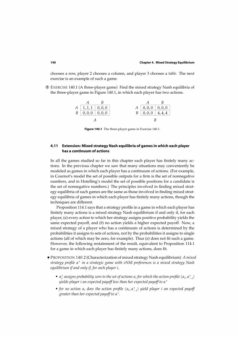
140 Chapter 4. Mixed Strategy Equilibrium
chooses a row, player 2 chooses a column, and player 3 chooses a table. The nextexercise is an example of such a game.
? EXERCISE 140.1 (A three-player game) Find the mixed strategy Nash equilibria ofthe three-player game in Figure 140.1, in which each player has two actions.
A B
A 1, 1, 1 0, 0, 0B 0, 0, 0 0, 0, 0
A
A B
A 0, 0, 0 0, 0, 0B 0, 0, 0 4, 4, 4
B
Figure 140.1 The three-player game in Exercise 140.1.
4.11 Extension: Mixed strategy Nash equilibria of games in which each player
has a continuum of actions
In all the games studied so far in this chapter each player has finitely many ac-tions. In the previous chapter we saw that many situations may conveniently bemodeled as games in which each player has a continuum of actions. (For example,in Cournot’s model the set of possible outputs for a firm is the set of nonnegativenumbers, and in Hotelling’s model the set of possible positions for a candidate isthe set of nonnegative numbers.) The principles involved in finding mixed strat-egy equilibria of such games are the same as those involved in finding mixed strat-egy equilibria of games in which each player has finitely many actions, though thetechniques are different.
Proposition 114.1 says that a strategy profile in a game in which each player hasfinitely many actions is a mixed strategy Nash equilibrium if and only if, for eachplayer, (a) every action to which her strategy assigns positive probability yields thesame expected payoff, and (b) no action yields a higher expected payoff. Now, amixed strategy of a player who has a continuum of actions is determined by theprobabilities it assigns to sets of actions, not by the probabilities it assigns to singleactions (all of which may be zero, for example). Thus (a) does not fit such a game.However, the following restatement of the result, equivalent to Proposition 114.1for a game in which each player has finitely many actions, does fit.
PROPOSITION 140.2 (Characterization of mixed strategy Nash equilibrium) A mixed
strategy profile α∗ in a strategic game with vNM preferences is a mixed strategy Nash
equilibrium if and only if, for each player i,
• α∗i assigns probability zero to the set of actions ai for which the action profile (ai, α∗
−i)
yields player i an expected payoff less than her expected payoff to α∗
• for no action ai does the action profile (ai, α∗−i) yield player i an expected payoff
greater than her expected payoff to α∗.

4.11 Extension: Mixed equilibria of games in which each player has a continuum of actions 141
A significant class of games in which each player has a continuum of actionsconsists of games in which each player’s set of actions is a one-dimensional inter-val of numbers. Consider such a game with two players; let player i’s set of actionsbe the interval from ai to ai, for i = 1, 2. Identify each player’s mixed strategy witha cumulative probability distribution on this interval. (See Section 17.6.4 in the ap-pendix on mathematics if you are not familiar with this notion.) That is, the mixedstrategy of each player i is a nondecreasing function Fi for which 0 ≤ Fi(ai) ≤ 1 forevery action ai; the number Fi(ai) is the probability that player i’s action is at mostai.
The form of a mixed strategy Nash equilibrium in such a game may be verycomplex. Some such games, however, have equilibria of a particularly simpleform, in which each player’s equilibrium mixed strategy assigns probability zeroexcept in an interval. Specifically, consider a pair (F1, F2) of mixed strategies thatsatisfies the following conditions for i = 1, 2.
• There are numbers xi and yi such that player i’s mixed strategy Fi assignsprobability zero except in the interval from xi to yi: Fi(z) = 0 for z < xi, andF(z) = 1 for z ≥ yi.
• Player i’s expected payoff when her action is ai and the other player uses hermixed strategy Fj takes the form
{= ci for xi ≤ ai ≤ yi
≤ ci for ai < xi and ai > yi
where ci is a constant.
(The second condition is illustrated in Figure 141.1.) By Proposition 140.2, such apair of mixed strategies, if it exists, is a mixed strategy Nash equilibrium of thegame, in which player i’s expected payoff is ci, for i = 1, 2.
a1 x1 y1 a1a1 →
c1
Player 1’s expected payoff given F2
a2 x2 y2 a2a2 →
c2
Player 2’s expected payoff given F1
Figure 141.1 If (i) F1 assigns positive probability only to actions in the interval from x1 to y1, (ii) F2assigns positive probability only to the actions in the interval from x2 to y2, (iii) given player 2’s mixedstrategy F2, player 1’s expected payoff takes the form shown in the left panel, and (iv) given player 1’smixed strategy F1, player 2’s expected payoff takes the form shown in the right panel, then (F1, F2) is amixed strategy equilibrium.
The next example illustrates how a mixed strategy equilibrium of such a gamemay be found. The example is designed to be very simple; be warned that in
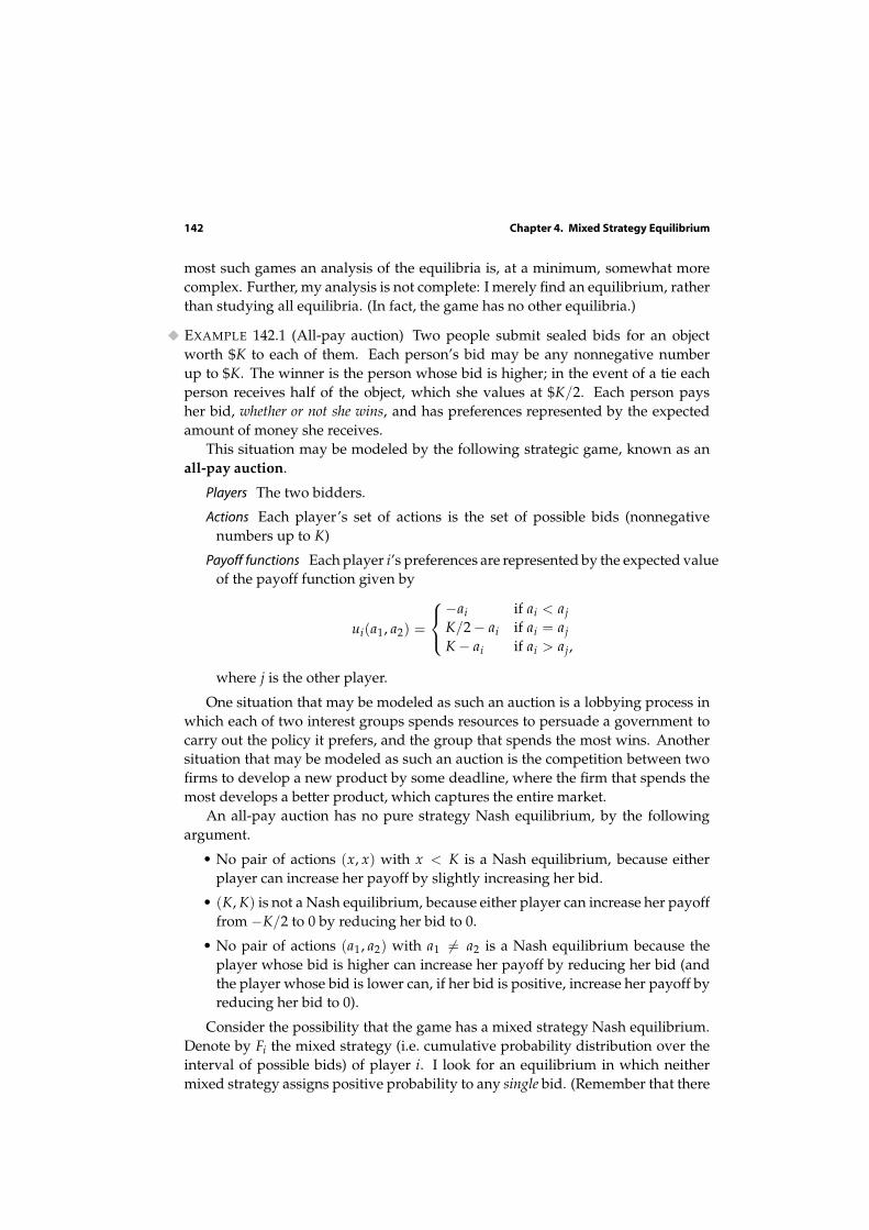
142 Chapter 4. Mixed Strategy Equilibrium
most such games an analysis of the equilibria is, at a minimum, somewhat morecomplex. Further, my analysis is not complete: I merely find an equilibrium, ratherthan studying all equilibria. (In fact, the game has no other equilibria.)
EXAMPLE 142.1 (All-pay auction) Two people submit sealed bids for an objectworth $K to each of them. Each person’s bid may be any nonnegative numberup to $K. The winner is the person whose bid is higher; in the event of a tie eachperson receives half of the object, which she values at $K/2. Each person paysher bid, whether or not she wins, and has preferences represented by the expectedamount of money she receives.
This situation may be modeled by the following strategic game, known as anall-pay auction.
Players The two bidders.
Actions Each player’s set of actions is the set of possible bids (nonnegativenumbers up to K)
Payoff functions Each player i’s preferences are represented by the expected valueof the payoff function given by
ui(a1, a2) =
−ai if ai < aj
K/2 − ai if ai = aj
K − ai if ai > aj,
where j is the other player.
One situation that may be modeled as such an auction is a lobbying process inwhich each of two interest groups spends resources to persuade a government tocarry out the policy it prefers, and the group that spends the most wins. Anothersituation that may be modeled as such an auction is the competition between twofirms to develop a new product by some deadline, where the firm that spends themost develops a better product, which captures the entire market.
An all-pay auction has no pure strategy Nash equilibrium, by the followingargument.
• No pair of actions (x, x) with x < K is a Nash equilibrium, because eitherplayer can increase her payoff by slightly increasing her bid.
• (K, K) is not a Nash equilibrium, because either player can increase her payofffrom −K/2 to 0 by reducing her bid to 0.
• No pair of actions (a1, a2) with a1 6= a2 is a Nash equilibrium because theplayer whose bid is higher can increase her payoff by reducing her bid (andthe player whose bid is lower can, if her bid is positive, increase her payoff byreducing her bid to 0).
Consider the possibility that the game has a mixed strategy Nash equilibrium.Denote by Fi the mixed strategy (i.e. cumulative probability distribution over theinterval of possible bids) of player i. I look for an equilibrium in which neithermixed strategy assigns positive probability to any single bid. (Remember that there

4.11 Extension: Mixed equilibria of games in which each player has a continuum of actions 143
are infinitely many possible bids.) In this case Fi(ai) is both the probability thatplayer i bids at most ai and the probability that she bids less than ai. I furtherrestrict attention to strategy pairs (F1, F2) for which, for i = 1, 2, there are numbersxi and yi such that Fi assigns positive probability only to the interval from xi to yi.
To investigate the possibility of such an equilibrium, consider player 1’s ex-pected payoff when she uses the action a1, given player 2’s mixed strategy F2.
• If a1 < x2 then a1 is less than player 2’s bid with probability one, so thatplayer 1’s payoff is −a1.
• If a1 > y2 then a1 exceeds player 2’s bid with probability one, so that player 1’spayoff is K − a1.
• If x2 ≤ a1 ≤ y2 then player 1’s expected payoff is calculated as follows. Withprobability F2(a1) player 2’s bid is less than a1, in which case player 1’s payoffis K − a1; with probability 1 − F2(a1) player 2’s bid exceeds a1, in which caseplayer 1’s payoff is −a1; and, by assumption, the probability that player 2’sbid is exactly equal to a1 is zero. Thus player 1’s expected payoff is
(K − a1)F2(a1) + (−a1)(1 − F2(a1)) = KF2(a1) − a1.
We need to find values of x2 and y2 and a strategy F2 such that player 1’s ex-pected payoff satisfies the condition illustrated in the left panel of Figure 141.1: itis constant on the interval from x1 to y1, and less than this constant for a1 < x1 anda1 > y1. The constancy of the payoff on the interval from x1 to y1 requires thatKF2(a1) − a1 = c1 for x1 ≤ a1 ≤ y1, for some constant c1. We also need F2(x2) = 0and F2(y2) = 1 (because I am restricting attention to equilibria in which neitherplayer’s strategy assigns positive probability to any single action), and F2 mustbe nondecreasing (so that it is a cumulative probability distribution). Analogousconditions must be satisfied by x2, y2, and F1.
We see that if x1 = x2 = 0, y1 = y2 = K, and F1(z) = F2(z) = z/K for all z with0 ≤ z ≤ K then all these conditions are satisfied. Each player’s expected payoff isconstant, equal to 0 for all her actions a1.
Thus the game has a mixed strategy Nash equilibrium in which each playerrandomizes “uniformly” over all her actions. In this equilibrium each player’sexpected payoff is 0: on average, the amount a player spends is exactly equal tothe value of the object. (A more involved argument shows that this equilibrium isthe only mixed strategy Nash equilibrium of the game.)
?? EXERCISE 143.1 (All-pay auction with many bidders) Consider the generalizationof the game considered in the previous example in which there are n ≥ 2 bidders.Find a mixed strategy Nash equilibrium in which each player uses the same mixedstrategy. (If you know how, find each player’s mean bid in the equilibrium.)
?? EXERCISE 143.2 (Bertrand’s duopoly game) Consider Bertrand’s oligopoly game(Section 3.2) when there are two firms. Assume that each firm’s preferences arerepresented by its expected profit. Show that if the function (p − c)D(p) is increas-ing in p, and increases without bound as p increases without bound, then for every

144 Chapter 4. Mixed Strategy Equilibrium
p > c, the game has a mixed strategy Nash equilibrium in which each firm usesthe same mixed strategy F, with F(p) = 0 and F(p) > 0 for p > p.
In the games in the example and exercises each player’s payoff depends onlyon her action and whether this action is greater than, equal to, or less than the otherplayers’ actions. The limited dependence of each player’s payoff on the other play-ers’ actions makes the calculation of a player’s expected payoff straightforward.In many games, each player’s payoff is affected more substantially by the otherplayers’ actions, making the calculation of expected payoff more complex; moresophisticated mathematical tools are required to analyze such games.
4.12 Appendix: Representing preferences over lotteries by the expected value
of a payoff function
4.12.1 Expected payoffs
Suppose that a decision-maker has preferences over a set of deterministic out-comes, and that each of her actions results in a lottery (probability distribution)over these outcomes. In order to determine the action she chooses, we need toknow her preferences over these lotteries. As argued in Section 4.1.3, we cannot de-
rive these preferences from her preferences over deterministic outcomes, but haveto specify them as part of the model.
So assume that we are given the decision-maker’s preferences over lotteries.As in the case of preferences over deterministic outcomes, under some fairly weakassumptions we can represent these preferences by a payoff function. (Refer toSection 1.2.2.) That is, when there are K deterministic outcomes we can find afunction, say U, over lotteries such that
U(p1, . . . , pK) > U(p′1, . . . , p′K)
if and only if the decision-maker prefers the lottery (p1, . . . , pK) to the lottery(p′1, . . . , p′K) (where (p1, . . . , pK) is the lottery in which outcome 1 occurs withprobability p1, outcome 2 occurs with probability p2, and so on).
For many purposes, however, we need more structure: we cannot get very farwithout restricting to preferences for which there is a more specific representation.The standard approach, developed by von Neumann and Morgenstern (1944), is toimpose an additional assumption—the “independence axiom”—that allows us toconclude that the decision-maker’s preferences can be represented by an expected
payoff function. More precisely, the independence axiom (which I do not describe)allows us to conclude that there is a payoff function u over deterministic outcomessuch that the decision-maker’s preference relation over lotteries is represented bythe function U(p1, . . . , pK) = ∑
Kk=1 pku(ak), where ak is the kth outcome of the
lottery:K
∑k=1
pku(ak) >K
∑k=1
p′ku(ak) (144.1)

4.12 Appendix: Representing preferences by expected payoffs 145
if and only if the decision-maker prefers the lottery (p1, . . . , pK) to the lottery(p′1, . . . , p′K). That is, the decision-maker evaluates a lottery by its expected pay-
off according to the function u, which is known as the decision-maker’s Bernoulli
payoff function.Suppose, for example, that there are three possible deterministic outcomes: the
decision-maker may receive $0, $1, or $5, and naturally prefers $5 to $1 to $0. Sup-pose that she prefers the lottery ( 1
2 , 0, 12 ) to the lottery (0, 3
4 , 14 ) (where the first
number in each list is the probability of $0, the second number is the probabilityof $1, and the third number is the probability of $5). This preference is consis-tent with preferences represented by the expected value of a payoff function u forwhich u(0) = 0, u(1) = 1, and u(5) = 4, because
12 · 0 + 1
2 · 4 > 34 · 1 + 1
4 · 4.
(Many other payoff functions are consistent with a preference for ( 12 , 0, 1
2 ) over(0, 3
4 , 14 ). Among those in which u(0) = 0 and u(5) = 4, for example, any function
for which u(1) < 43 does the job.) Suppose, on the other hand, that the decision-
maker prefers the lottery (0, 34 , 1
4 ) to the lottery ( 12 , 0, 1
2 ). This preference is consis-tent with preferences represented by the expected value of a payoff function u forwhich u(0) = 0, u(1) = 3, and u(5) = 4, because
12 · 0 + 1
2 · 4 < 34 · 3 + 1
4 · 4.
? EXERCISE 145.1 (Preferences over lotteries) There are three possible outcomes; inthe outcome ai a decision-maker gains $ai, where a1 < a2 < a3. The decision-maker prefers a3 to a2 to a1 and she prefers the lottery (0.3, 0, 0.7) to (0.1, 0.4, 0.5)
to (0.3, 0.2, 0.5) to (0.45, 0, 0.55). Is this information consistent with the decision-maker’s preferences being represented by the expected value of a payoff function?If so, find a payoff function consistent with the information. If not, show whynot. Answer the same questions when, alternatively, the decision-maker prefersthe lottery (0.4, 0, 0.6) to (0, 0.5, 0.5) to (0.3, 0.2, 0.5) to (0.45, 0, 0.55).
Preferences represented by the expected value of a (Bernoulli) payoff functionhave the great advantage that they are completely specified by that payoff func-tion. Once we know u(ak) for each possible outcome ak we know the decision-maker’s preferences among all lotteries. This significant advantage does, how-ever, carry with it a small price: it is very easy to confuse a Bernoulli payoff func-tion with a payoff function that represents the decision-maker’s preferences overdeterministic outcomes.
To describe the relation between the two, suppose that a decision-maker’s pref-erences over lotteries are represented by the expected value of the Bernoulli pay-off function u. Then certainly u is a payoff function that represents the decision-maker’s preferences over deterministic outcomes (which are special cases of lotter-ies, in which a single outcome is assigned probability 1). However, the converse isnot true: if the decision-maker’s preferences over deterministic outcomes are repre-sented by the payoff function u (i.e. the decision-maker prefers a to a′ if and only if

146 Chapter 4. Mixed Strategy Equilibrium
u(a) > u(a′)), then u is not necessarily a Bernoulli payoff function whose expectedvalue represents the decision-maker’s preferences over lotteries. For instance, sup-pose that the decision-maker prefers $5 to $1 to $0, and prefers the lottery ( 1
2 , 0, 12 )
to the lottery (0, 34 , 1
4 ). Then her preferences over deterministic outcomes are con-sistent with the payoff function u for which u(0) = 0, u(1) = 3, and u(5) = 4.However, her preferences over lotteries are not consistent with the expected valueof this function (since 1
2 · 0 + 12 · 4 < 3
4 · 3 + 14 · 4). The moral is that you should be
careful to determine the type of payoff function you are dealing with.
4.12.2 Equivalent Bernoulli payoff functions
If a decision-maker’s preferences in a deterministic environment are representedby the payoff function u then they are represented also by any payoff function thatis an increasing function of u (see Section 1.2.2). The analogous property is notsatisfied by Bernoulli payoff functions. Consider the example discussed above. ABernoulli payoff function u for which u(0) = 0, u(1) = 1, and u(5) = 4 is consistentwith a preference for the lottery ( 1
2 , 0, 12 ) over (0, 3
4 , 14 ), but the function
√u, for
which u(0) = 0, u(1) = 1, and u(5) = 2, is not consistent with such a preference( 1
2 · 0 + 12 · 2 < 3
4 · 1 + 14 · 2), though the square root function is increasing (larger
numbers have larger square roots).Under what circumstances do the expected values of two Bernoulli payoff func-
tions represent the same preferences? The next result shows that they do so if andonly if one payoff function is an increasing linear function of the other.
LEMMA 146.1 (Equivalence of Bernoulli payoff functions) Suppose there are at least
three possible outcomes. The expected values of the Bernoulli payoff functions u and v
represent the same preferences over lotteries if and only if there exist numbers η and θ with
θ > 0 such that u(x) = η + θv(x) for all x.
If the expected value of u represents a decision-maker’s preferences over lot-teries then so, for example, do the expected values of 2u, 1 + u, and −1 + 4u; butthe expected values of u2 and of
√u do not.
Part of the lemma is easy to establish. Let u be a Bernoulli payoff functionwhose expected value represents a decision-maker’s preferences, and let v(x) =
η + θu(x) for all x, where η and θ are constants with θ > 0. I argue that the expectedvalues of u and of v represent the same preferences. Suppose that the decision-maker prefers the lottery (p1, . . . , pK) to the lottery (p′1, . . . , p′K). Then her expectedpayoff to (p1, . . . , pK) exceeds her expected payoff to (p′
1, . . . , p′K), or
K
∑k=1
pku(ak) >K
∑k=1
p′ku(ak) (146.2)
(see (144.1)). Now,
K
∑k=1
pkv(ak) =K
∑k=1
pkη +K
∑k=1
pkθu(ak) = η + θK
∑k=1
pku(ak),
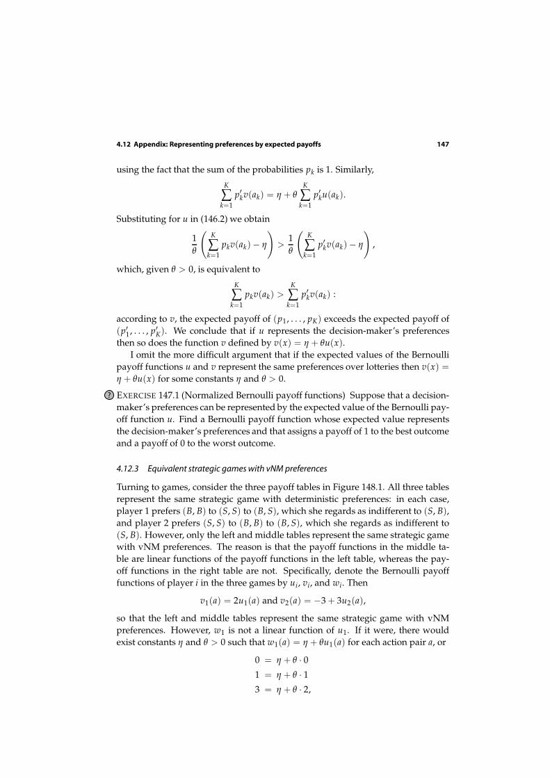
4.12 Appendix: Representing preferences by expected payoffs 147
using the fact that the sum of the probabilities pk is 1. Similarly,
K
∑k=1
p′kv(ak) = η + θK
∑k=1
p′ku(ak).
Substituting for u in (146.2) we obtain
1θ
(K
∑k=1
pkv(ak) − η
)
>1θ
(K
∑k=1
p′kv(ak) − η
)
,
which, given θ > 0, is equivalent to
K
∑k=1
pkv(ak) >K
∑k=1
p′kv(ak) :
according to v, the expected payoff of (p1, . . . , pK) exceeds the expected payoff of(p′1, . . . , p′K). We conclude that if u represents the decision-maker’s preferencesthen so does the function v defined by v(x) = η + θu(x).
I omit the more difficult argument that if the expected values of the Bernoullipayoff functions u and v represent the same preferences over lotteries then v(x) =
η + θu(x) for some constants η and θ > 0.
? EXERCISE 147.1 (Normalized Bernoulli payoff functions) Suppose that a decision-maker’s preferences can be represented by the expected value of the Bernoulli pay-off function u. Find a Bernoulli payoff function whose expected value representsthe decision-maker’s preferences and that assigns a payoff of 1 to the best outcomeand a payoff of 0 to the worst outcome.
4.12.3 Equivalent strategic games with vNM preferences
Turning to games, consider the three payoff tables in Figure 148.1. All three tablesrepresent the same strategic game with deterministic preferences: in each case,player 1 prefers (B, B) to (S, S) to (B, S), which she regards as indifferent to (S, B),and player 2 prefers (S, S) to (B, B) to (B, S), which she regards as indifferent to(S, B). However, only the left and middle tables represent the same strategic gamewith vNM preferences. The reason is that the payoff functions in the middle ta-ble are linear functions of the payoff functions in the left table, whereas the pay-off functions in the right table are not. Specifically, denote the Bernoulli payofffunctions of player i in the three games by ui, vi, and wi. Then
v1(a) = 2u1(a) and v2(a) = −3 + 3u2(a),
so that the left and middle tables represent the same strategic game with vNMpreferences. However, w1 is not a linear function of u1. If it were, there wouldexist constants η and θ > 0 such that w1(a) = η + θu1(a) for each action pair a, or
0 = η + θ · 0
1 = η + θ · 1
3 = η + θ · 2,

148 Chapter 4. Mixed Strategy Equilibrium
but these three equations have no solution. Thus the left and right tables representdifferent strategic games with vNM preferences. (As you can check, w2 is not alinear function of u2 either; but for the games not to be equivalent it is sufficientthat one player’s preferences be different.) Another way to see that player 1’s vNMpreferences in the left and right games are different is to note that in the left tableplayer 1 is indifferent between the certain outcome (S, S) and the lottery in which(B, B) occurs with probability 1
2 and (S, B) occurs with probability 12 (each yields
an expected payoff of 1), whereas in the right table she prefers the latter (since ityields an expected payoff of 1.5).
B S
B 2, 1 0, 0S 0, 0 1, 2
B S
B 4, 0 0, −3S 0, −3 2, 3
B S
B 3, 2 0, 1S 0, 1 1, 4
Figure 148.1 All three tables represent the same strategic game with ordinal preferences, but only theleft and middle games, not the right one, represent the same strategic game with vNM preferences.
? EXERCISE 148.1 (Games equivalent to the Prisoner’s Dilemma) Which of the tablesin Figure 148.2 represents the same strategic game with vNM preferences as thePrisoner’s Dilemma as specified in the left panel of Figure 104.1, when the numbersare interpreted as Bernoulli payoffs?
C D
C 3, 3 0, 4D 4, 0 2, 2
C D
C 6, 0 0, 2D 9, −4 3, −2
Figure 148.2 The payoff tables for Exercise 148.1.
Notes
The ideas behind mixed strategies and preferences represented by expected pay-offs date back in Western thought at least to the eighteenth century (see Guil-baud (1961) and Kuhn (1968), and Bernoulli (1738), respectively). The modernformulation of a mixed strategy is due to Borel (1921; 1924, 204–221; 1927); themodel of the representation of preferences by an expected payoff function is dueto von Neumann and Morgenstern (1944, 15–31; 1947, 617–632). The model ofa mixed strategy Nash equilibrium and Proposition 117.1 on the existence of amixed strategy Nash equilibrium in a finite game are due to Nash (1950a, 1951).Proposition 120.1 is an implication of the existence of a “trembling hand perfectequilibrium”, due to Selten (1975, Theorem 5).
The example in the box on page 102 is taken from Allais (1953). Conlisk (1989)discusses some of the evidence on the theory of expected payoffs; Machina (1987)and Hey (1997) survey the subject. (The purchasing power of the largest prize inAllais’ example was roughly US$6.6m in 1989 (the date of Conlisk’s paper, in which

Notes 149
the prize is US$5m) and roughly US$8m in 1999.) The model in Section 4.6 is due toPitchik and Schotter (1987). The model in Section 4.8 is a special case of the one inPalfrey and Rosenthal (1984); the interpretation and analysis that I describe is takenfrom an unpublished 1984 paper of William F. Samuelson. The box on page 131draws upon Rosenthal (1964), Latané and Nida (1981), Brown (1986), and Aron-son (1995). Best response dynamics were first studied by Cournot (1838, Ch. VII),in the context of his duopoly game. Fictitious play was suggested by Brown (1951).Robinson (1951) shows that the process converges to a mixed strategy Nash equi-librium in any two-player game in which the players’ interests are opposed; Shap-ley (1964, Section 5) exhibits a game outside this class in which the process doesnot converge. Recent work on learning in games is surveyed by Fudenberg andLevine (1998).
The game in Exercise 115.2 is due to David L. Silverman (see Silverman 1981–82 and Heuer 1995). Exercise 116.1 is based on Palfrey and Rosenthal (1983). Exer-cise 116.2 is taken from Shubik (1982, 226) (who finds only one of the continuumof equilibria of the game).
The model in Exercise 126.1 is taken from Peters (1984). Exercise 127.3 is a vari-ant of an exercise of Moulin (1986, 167, 185). Exercise 130.3 is based on Palfrey andRosenthal (1984). The game Rock-Paper-Scissors (Exercise 139.1) was first studiedby Borel (1924) and von Neumann (1928). Exercise 139.2 is based on Karlin (1959a,92–94), who attributes the game to an unpublished paper by Dresher.
Exercise 143.1 is based on a result in Baye, Kovenock, and de Vries (1996). Themixed strategy Nash equilibria of Bertrand’s model of duopoly (Exercise 143.2) arestudied in detail by Baye and Morgan (1999).
The method of finding all mixed strategy equilibrium described in Section 4.10is computationally very intense in all but the simplest games. Some computation-ally more efficient methods are implemented in the computer program GAMBIT,located at www.hss.caltech.edu/~gambit/Gambit.html.