4. MORE ABOUT THE MODEL1

4.1 LEAD BIOAVAILABILITY

4.1.1 Background

The concept of bioavailability is important for site-specific risk assessments for lead. The concept springs from the fact that lead potentially available to produce harm and found in exposure pathways or in body receiving compartments (lung, skin, gut) must reach the biological sites of action in order for an adverse health effect to occur in exposed humans or ecological biota.

This section focuses primarily on the bioavailability of inorganic lead from soils and dusts. Lead bioavailability from air and drinking water is also important and is discussed in limited detail below. In order to provide coherent and useful guidance to the reader and user of this chapter, it is subdivided into (1) introductory material that includes definitions of bioavailability and resource material in the technical literature; (2) the close lead absorption­bioavailability relationships, including the physiological and biochemical mechanisms of lead absorption and the many, complex factors that influence such uptake; (3) the main focus of the chapter, bioavailability as it relates to human and experimental toxicology, including the various biophysico-chemical and environmental aspects of the lead exposure matrix, methodological approaches in toxicology for quantifying bioavailability, the increasingly important question of relevant experimental animal models for quantifying lead bioavailability in humans; and, finally, (4) a summary and critical overview, which attempts to spell out the appropriate uses of bioavailability information and limits to use this information in site-specific risk assessment.

4.1.2 Definitions

A clear agreement on a definition of bioavailability should be established before one presents a detailed discussion of this topic. The difficulty here is that there are various

1This chapter is intended to provide guidance on some technically advanced applications of the model. We have attempted to provide the best scientific documentation available but recognize that new information may become available in these rapidly advancing fields. The user is referred to Section 1.6 for information on how to get additional and more up-to-date assistance with specific applications of the model.

4-1

definitions of bioavailability depending on the scientific discipline using the term and the technical context of use.

Typically, the pharmacologist or toxicologist or others in biomedical disciplines are concerned with measuring bioavailability as that fraction of the total amount of material in contact with a body portal of entry (lung, gut, skin) that then enters the blood. For the purpose of describing the Integrated Exposure Uptake Biokinetic (IEUBK) Model, this is the definition to be used in this manual. However, an aquatic biologist may define bioavailability as that fraction of material solubilized in the water column under certain conditions of hardness and pH. An aquatic toxicologist might consider contaminants which are soluble under specific stream conditions to be bioavailable to fish or benthic organisms. A biochemist or biochemical toxicologist would consider bioavailability with reference to that fraction of a toxicant which is available at the organ or cellular site of toxicity.

The above definitions can be viewed as dosimetrically descriptive. There are quantitative methodological definitions that figure as well. As described later, bioavailability can be defined as being absolute or relative (comparative). Absolute bioavailability, for example, is the amount of substance entering the blood via a particular biological pathway relative to the absolute amount that has been ingested. Relative bioavailability of lead is indexed by comparing the bioavailability of one chemical species or form of lead with that of another form of lead. A second methodological description for bioavailability that is used by toxicologists is the ratio of areas under the dose-response curve for either of two forms of lead, or two methods of administration. Typically, the latter involves comparing injected with orally administered doses.

4.1.3 Literature Sources on Bioavailability

More detailed reviews and discussions of the topic of lead bioavailability in humans and experimental animals have been presented by Mushak (1991) and Chaney et al. (1988). As is evident from these reviews, our present understanding of lead bioavailability has developed from both human and animal studies. For further in-depth discussion of the various components of bioavailability, for example, lead absorption, the reader is also referred to the following documents: (1) the Air Quality Criteria Document for Lead (U.S. Environmental Protection Agency, 1986), and (2) the Proceedings of the Symposium on the Bioavailability and Dietary Exposure of Lead (1991).

4-2

Citations of key specific studies are provided in the relevant sections and subsections of this chapter rather than here, so as to be less disruptive to the reader.

4.1.4 Lead Absorption-Bioavailability Relationships

By definition, the absorption (uptake) of lead into the circulation is the critical kinetic component of the overall process called bioavailability. Not only the amount, but also the rate of uptake of that given amount is important, particularly under acute or subacute exposure conditions, and when dealing with lead-containing media in the gastrointestinal (GI) tract. Such material is itself moving through the GI tract within a relatively short time period. Consequently, the biological and physiological characteristics of absorption, the subcellular mechanisms of absorption, and the factors influencing its occurrence must be understood in order to understand the resulting phenomenon. The focus of this chapter is soil and dust lead ingested (swallowed) by populations at risk, requiring that lead uptake phenomena in the gastrointestinal tract be given most of the attention.

Species-specific anatomical and physiological determinants of GI absorption are the macroscopic factors that provide the basic means by which lead absorption occurs. As noted in more detail in Section 4.1.5, there are major structural differences in the anatomy of the GI tract of various mammalian species that would affect lead absorption. Similarly, it is the physiology of the mucosal lining (epithelium) of the mammalian GI tract that is the first dynamic determinant of lead movement from the GI tract to the bloodstream.

4.1.5 Cellular and Subcellular Mechanisms of Lead Absorption

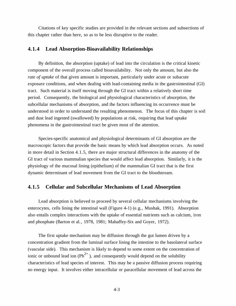
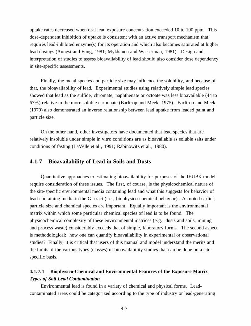
Lead absorption is believed to proceed by several cellular mechanisms involving the enterocytes, cells lining the intestinal wall (Figure 4-1) (e.g., Mushak, 1991). Absorption also entails complex interactions with the uptake of essential nutrients such as calcium, iron and phosphate (Barton et al., 1978, 1981; Mahaffey-Six and Goyer, 1972).

The first uptake mechanism may be diffusion through the gut lumen driven by a concentration gradient from the luminal surface lining the intestine to the basolateral surface (vascular side). This mechanism is likely to depend to some extent on the concentration of ionic or unbound lead ion (Pb2+), and consequently would depend on the solubility characteristics of lead species of interest. This may be a passive diffusion process requiring no energy input. It involves either intracellular or paracellular movement of lead across the

4-3

Lumen

Pb-complex Pb++

Microvilli

Tight Junction

Terminal Web

Enterocyte

Desmosome

Pb-carrier

Tight Junction

Intermediate Junction

Intercellular Space

Pb++

Pb-carrier

Pb++

Pb++ Pb++

Pb++

Pb++

Pb++

Basement Membrane

Figure 4-1. Schematic drawing of the enterocyte showing possible mechanisms for lead absorption. Possible mechanisms include: (1) an active or facilitated component; (2) a transcellular component perhaps involving pinocytotic mechanisms; and (3) a diffusion-driven paracellular route across tight junctions.

Source: Mushak, 1991, adapted from Morton et al. (1985).

wall. Paracellular transport would entail movement across the area between cells called "tight junctions."

In the second possibility, lead may enter the gut tissue (but not necessarily the bloodstream) by pinocytosis or other vesicular mechanisms. In pinocytosis, lead-bearing media in a liquid micro region of the gut are engulfed by the (enterocyte) cell membrane. Such encapsulating may involve lead in either a truly soluble or an emulsified/suspended form that is then carried to blood or to sites of toxic action. This process is biochemically analogous to handling of solid particles in phagocytosis.

Perhaps the quantitatively most important transport mechanism in environmental exposures typical for most individuals is energy-driven active transport, exploiting homeostatic transport mechanisms in place for calcium and iron transport (e.g., calcium binding protein [CaBP] or calbindin D), and under control of an enzyme—calcium, magnesium-dependent ATPase (Ca2+, Mg2+-ATPase)—involved in the absorption and regulation of blood calcium levels and located in the basolateral membrane of mucosal

4-4

epithelial cells. This active component of lead absorption displays a strong age dependence, being more important at younger ages. It is interesting that some of the transport systems that bring calcium into the body seem to have an even higher affinity for lead than for calcium (e.g., Fullmer et al., 1985).

While the results of experimental studies can be described quantitatively, the precise nature of biological and biochemical mechanisms in lead bioavailability is not yet completely understood. There is, however, a useful characterization of lead absorption mechanisms as either saturable (facilitated) or nonsaturable (passive). These various and complex biochemical/cellular mechanisms obviously have important implications for experimental models of human lead bioavailability, particularly with reference to comparison of in vivo to in vitro simple chemical simulation models.

4.1.6 Factors Affecting Lead Absorption

Lead uptake, especially from the GI tract, does not occur in a physiological vacuum but is the outcome of a complex set of interactions with other inorganic and organic substances, particularly such nutrients as calcium, iron, phosphate, vitamin D, fats, etc., as they occur in meals or with intermittent eating. In addition, uptake is a function of developmental stage (age), administered dose, the chemical species and the particle size of the lead-containing media.

It is well known that lead uptake is markedly lower with consumption of meals than under fasting conditions in adults (e.g., James et al., 1985; Rabinowitz et al., 1980) and presumably in children as well. Human data, in the aggregate, indicate that calcium, iron and other cations interact strongly as competitors to lead uptake so that lead uptake generally increases as dietary levels of these nutrients decrease (Mushak, 1991; U.S. Environmental Protection Agency, 1986). In rats, Garber and Wei (1974) showed that fasting increased the amount of lead taken up by the gut. Children are likely to be exposed to lead under a variety of fed or fasted (between meal) conditions. Therefore, any interpretations of lead bioavailability studies of site-specific characteristics should include the effect on uptake of food and time since eating.

There is a developmental or age dependency for the extent of lead absorption in both humans and experimental animals (Mushak, 1991; U.S. Environmental Protection Agency, 1986). Prepubertal children absorb more lead than do adults (Alexander et al., 1973; Ziegler et al., 1978). Experimental animal studies support the human data. Studies using rats

4-5

showed that pre-weanling animals absorb 40 to 50 times more of a given dose of lead than do adult animals (Kostial et al., 1971, 1978; Forbes and Reina, 1972), while infant monkeys will absorb 16 to 21 times more lead than adult monkeys (Munro et al., 1975). Possible mechanisms for this age dependence have been discussed (Weis and LaVelle, 1991; Mushak, 1991). The design or interpretation of bioavailability studies, aimed at assessing lead absorption for children, must consider age dependence of uptake of lead in any adjustments of the bioavailability parameter in the UBK model.

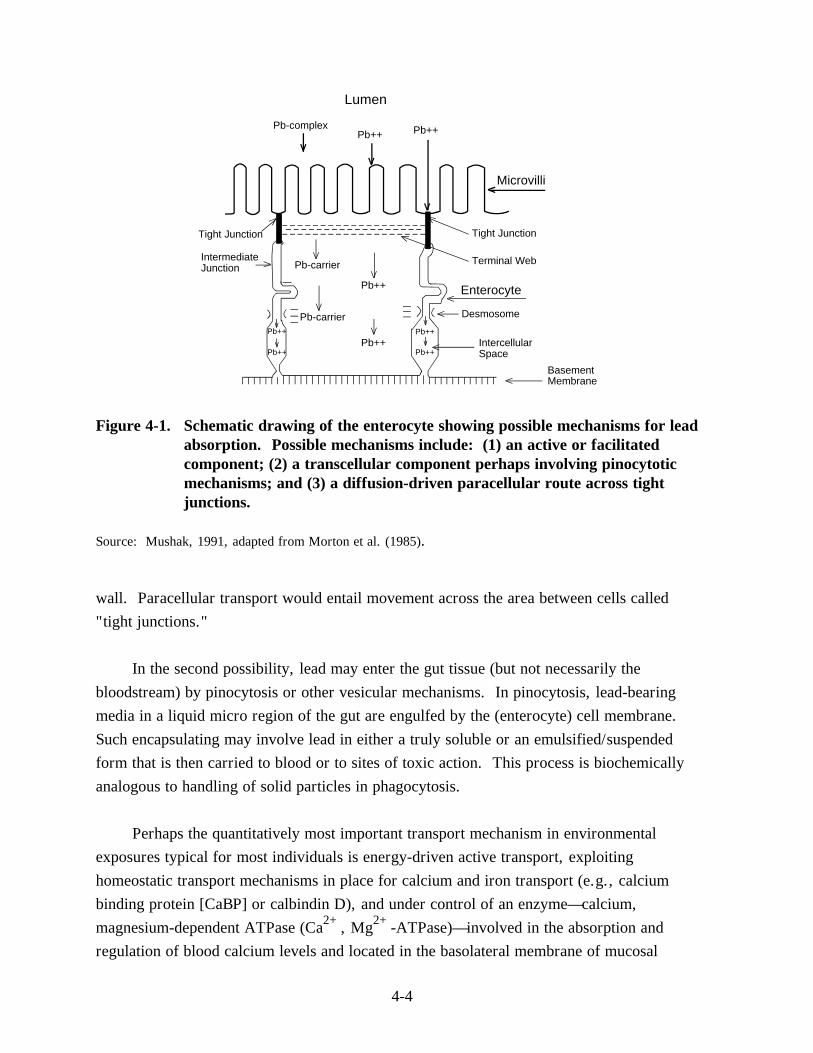
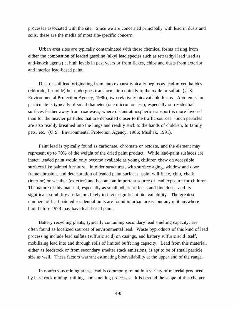
Human data indicate a dose dependence to the absorption of lead (Sherlock and Quinn, 1986). In duplicate diet studies of bottle-fed infants (5 to 7 kg) exposed to lead in water and in formula mixed with contaminated water, Sherlock and Quinn were able to quantify the dose dependence of lead absorption. Over the exposure range investigated in the study (40 to 3,000 Fg/week), these investigators determined that the relationship between blood lead concentration and lead intake was curvilinear (Figure 4-2). This opportunistic human data describing the dose-dependence of lead absorption was considered by the Agency when establishing the kinetic approach to lead absorption used in the IEUBK Model.

35

Mean and standard error

30

25

20

15

10

5

0 0 0.5 1.0 1.5 2.0 2.5

Lead intake (mg/week)

Figure 4-2. Dose-dependent relationship between dietary lead (formula mixed with water) and blood lead in infants.

Source: Sherlock and Quinn (1986).

Animal studies (e.g., Bushnell and DeLuca, 1983) indicate that GI lead absorption shows dependence on the level of oral dosing. Bushnell and DeLuca reported that lead

4-6

uptake rates decreased when oral lead exposure concentration exceeded 10 to 100 ppm. This dose-dependent inhibition of uptake is consistent with an active transport mechanism that requires lead-inhibited enzyme(s) for its operation and which also becomes saturated at higher lead dosings (Aungst and Fung, 1981; Mykkanen and Wasserman, 1981). Design and interpretation of studies to assess bioavailability of lead should also consider dose dependency in site-specific assessments.

Finally, the metal species and particle size may influence the solubility, and because of that, the bioavailability of lead. Experimental studies using relatively simple lead species showed that lead as the sulfide, chromate, naphthenate or octoate was less bioavailable (44 to 67%) relative to the more soluble carbonate (Barltrop and Meek, 1975). Barltrop and Meek (1979) also demonstrated an inverse relationship between lead uptake from leaded paint and particle size.

On the other hand, other investigators have documented that lead species that are relatively insoluble under simple in vitro conditions are as bioavailable as soluble salts under conditions of fasting (LaVelle et al., 1991; Rabinowitz et al., 1980).

4.1.7 Bioavailability of Lead in Soils and Dusts

Quantitative approaches to estimating bioavailability for purposes of the IEUBK model require consideration of three issues. The first, of course, is the physicochemical nature of the site-specific environmental media containing lead and what this suggests for behavior of lead-containing media in the GI tract (i.e., biophysico-chemical behavior). As noted earlier, particle size and chemical species are important. Equally important is the environmental matrix within which some particular chemical species of lead is to be found. The physicochemical complexity of these environmental matrices (e.g., dusts and soils, mining and process waste) considerably exceeds that of simple, laboratory forms. The second aspect is methodological: how one can quantify bioavailability in experimental or observational studies? Finally, it is critical that users of this manual and model understand the merits and the limits of the various types (classes) of bioavailability studies that can be done on a site-specific basis.

4.1.7.1 Biophysico-Chemical and Environmental Features of the Exposure Matrix Types of Soil Lead Contamination

Environmental lead is found in a variety of chemical and physical forms. Lead-contaminated areas could be categorized according to the type of industry or lead-generating

4-7

processes associated with the site. Since we are concerned principally with lead in dusts and soils, these are the media of most site-specific concern.

Urban area sites are typically contaminated with those chemical forms arising from either the combustion of leaded gasoline (alkyl lead species such as tetraethyl lead used as anti-knock agents) at high levels in past years or from flakes, chips and dusts from exterior and interior lead-based paint.

Dust or soil lead originating from auto exhaust typically begins as lead-mixed halides (chloride, bromide) but undergoes transformation quickly to the oxide or sulfate (U.S. Environmental Protection Agency, 1986), two relatively bioavailable forms. Auto emission particulate is typically of small diameter (one micron or less), especially on residential surfaces farther away from roadways, where distant atmospheric transport is more favored than for the heavier particles that are deposited closer to the traffic sources. Such particles are also readily breathed into the lungs and readily stick to the hands of children, to family pets, etc. (U.S. Environmental Protection Agency, 1986; Mushak, 1991).

Paint lead is typically found as carbonate, chromate or octoate, and the element may represent up to 70% of the weight of the dried paint product. While lead-paint surfaces are intact, leaded paint would only become available as young children chew on accessible surfaces like painted furniture. In older structures, with surface aging, window and door frame abrasion, and deterioration of leaded paint surfaces, paint will flake, chip, chalk (interior) or weather (exterior) and become an important source of lead exposure for children. The nature of this material, especially as small adherent flecks and fine dusts, and its significant solubility are factors likely to favor significant bioavailability. The greatest numbers of lead-painted residential units are found in urban areas, but any unit anywhere built before 1978 may have lead-based paint.

Battery recycling plants, typically containing secondary lead smelting capacity, are often found as localized sources of environmental lead. Waste byproducts of this kind of lead processing include lead sulfate (sulfuric acid) on casings, and battery sulfuric acid itself, mobilizing lead into and through soils of limited buffering capacity. Lead from this material, either as feedstock or from secondary smelter stack emissions, is apt to be of small particle size as well. These factors warrant estimating bioavailability at the upper end of the range.

In nonferrous mining areas, lead is commonly found in a variety of material produced by hard rock mining, milling, and smelting processes. It is beyond the scope of this chapter

4-8

to present a detailed discussion of lead contamination with nonferrous mining, milling and smelting. The reader is referred to the review by Mushak (1991) for further details.

Mining waste can be broadly characterized as: (1) waste rock; (2) mill tailings; and (3) smelting waste. Waste rock is that material removed from the mine but having insufficient mineral economic value to warrant processing. This material is typically discarded at openings to the mine, consists of larger particles, and may or may not be enriched in heavy metals.

Mill tailing is material that has been processed by a variety of physical grinding, separating and enrichment processes. This material typically has smaller particle size than the less processed wastes and the material is enriched in toxic elements, including lead. Mineral content depends on the characteristics of the ore body and the milling process, and may range from soluble carbonates (Ksp . 10-8) to extremely insoluble phosphates (Ksp .

10-80) of lead. Furthermore, lead that is associated with mining waste may either be freely exposed at the particle surface or entirely encapsulated, so that the lead is not available to be dissolved in simple solvents like water.

Smelting waste may exist in many forms. Air- and water-quenched slags are strikingly different in their physical nature. Water-quenched material is typically of fine particle size, while air quenching results in large chunks of oxidized slag. Chemically, these slags consist of various metal oxides and include lead and silicon oxides. Bag house dust consists of the fine particulate matter trapped in the emissions stream by a simple bag filter prior to leaving the stack. This material is very high in toxic metal content, including lead, and occurs in very small particle size. These small particles include lead sulfate and oxide species. Dross is the foam or lighter fraction of the liquid product of the floatation process. When cool, it may be discarded, resulting in a potentially important exposure source.

4.1.7.2 Is There a Better Way To Classify Lead-Contaminated Sites? It is often convenient to discuss lead-contaminated sites by classifying them as mining,

smelting, urban or battery sites. As our understanding of the complexities of lead-contaminated sites improves, it becomes less and less useful to use these simplified descriptions. For example, mining areas typically are associated with present or historical milling and smelting. Significant smelter-related contamination may remain at closed and operating mines that can contribute to typical mine waste exposure concerns.

4-9

Mine wastes may consist of lead in a multitude of physical and chemical forms as discussed above, making generalizations about exposure or potential exposure (and bioavailability) inappropriate without additional applied research data. Mining and smelting areas may share exposure sources often associated with such urban areas. Adequate characterization of lead-contaminated media, for the purpose of estimating bioavailability, should include assessment of physical and chemical parameters (e.g., particle size and appropriate media solubility) as well as biophysico-chemical characteristics. Generalizations regarding the source of lead contamination which do not address risk-specific details of the physicochemical and biochemical nature of the waste are not as useful for predicting health risks from exposures.

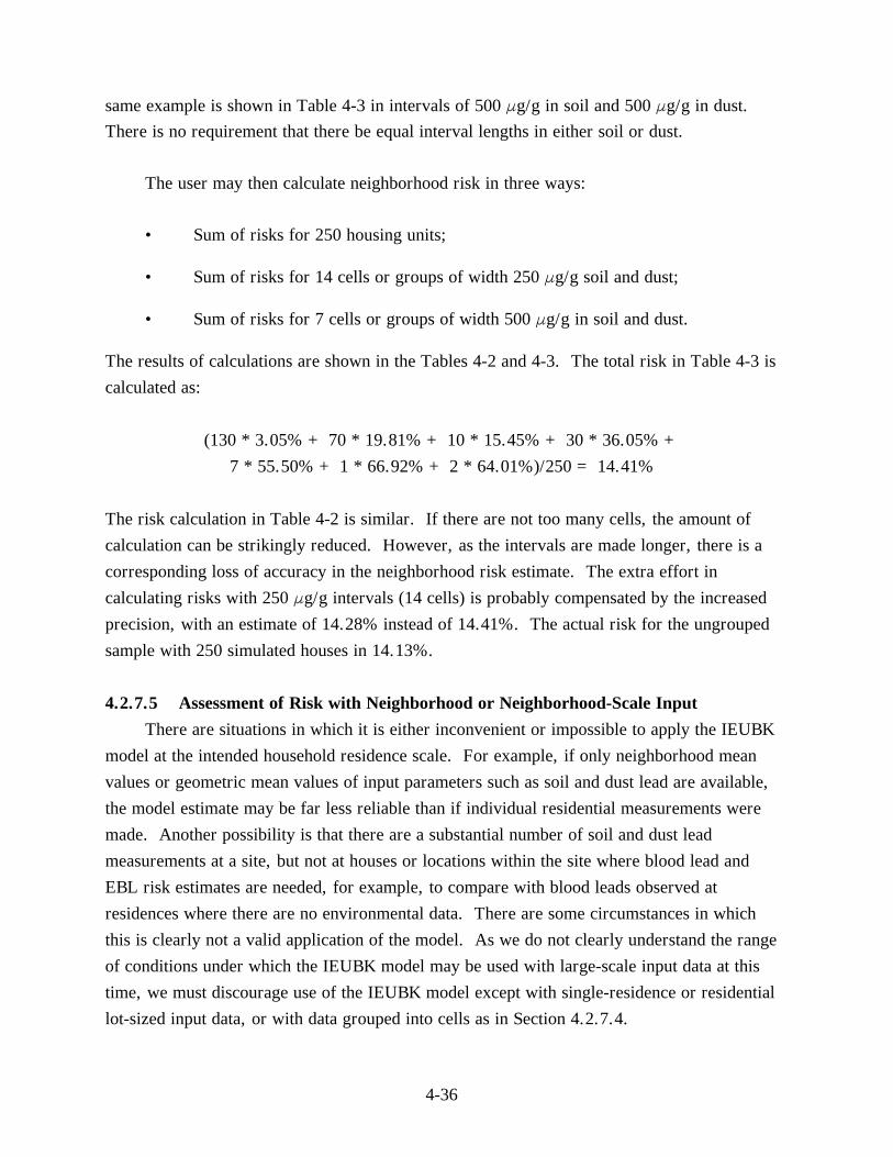
4.1.7.3 Methodological Approaches to Quantifying Bioavailability While lead can have severe toxic effects following a single very high exposure, we are

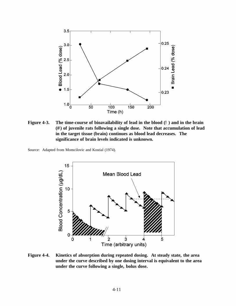
primarily concerned in this chapter with relatively low levels of average exposure and average blood lead concentration (see Figures 4-3 and 4-4 for single versus multiple exposures and target organ concentrations).

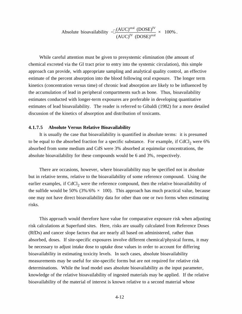
The average near steady state (pseudoequilibrium) of an accumulating toxicant such as lead in blood following chronic (repetitive) exposure is proportional to the amount absorbed during each exposure. At low ingestion rates, where absorption and biokinetic processes are nearly linear, the following relationship applies between changes in blood lead and changes in chronic exposure:

) PbB ' ) Pb&abs./day ( mean residence time in blood pool . volume of distribution in blood pool

Methods used to describe the fraction absorbed from exposure are well established and will be the primary focus of the following discussion.

4.1.7.4 Determination of Absolute Bioavailability The methodology for quantifying absolute bioavailability in toxicology commonly

compares (a) the area under the time-versus-blood-concentration curve (AUC) following intravenous (IV) injection with (b) an equivalent dose and a similar AUC measurement following ingestion of the substance being investigated. The ratio of AUCoral to AUCIV is then taken as a measure of percent absorption in the gut. From this, absolute bioavailability over a short time frame may be defined as:

4-10

4-11

Figure 4-3. The time-course of bioavailability of lead in the blood (!!) and in the brain(##) of juvenile rats following a single dose. in the target tissue (brain) continues as blood lead decreases. significance of brain levels indicated is unknown.

Source:

Figure 4-4. Kinetics of absorption during repeated dosing. under the curve described by one dosing interval is equivalent to the areaunder the curve following a single, bolus dose.

Note that accumulation of leadThe

Adapted from Momcilovic and Kostial (1974).

At steady state, the area

Absolute bioavailability ' (AUC)oral (DOSE)IV × 100%.

(AUC)IV (DOSE)oral

While careful attention must be given to presystemic elimination (the amount of chemical excreted via the GI tract prior to entry into the systemic circulation), this simple approach can provide, with appropriate sampling and analytical quality control, an effective estimate of the percent absorption into the blood following oral exposure. The longer term kinetics (concentration versus time) of chronic lead absorption are likely to be influenced by the accumulation of lead in peripheral compartments such as bone. Thus, bioavailability estimates conducted with longer-term exposures are preferable in developing quantitative estimates of lead bioavailability. The reader is referred to Gibaldi (1982) for a more detailed discussion of the kinetics of absorption and distribution of toxicants.

4.1.7.5 Absolute Versus Relative Bioavailability It is usually the case that bioavailability is quantified in absolute terms: it is presumed

to be equal to the absorbed fraction for a specific substance. For example, if CdCl2 were 6% absorbed from some medium and CdS were 3% absorbed at equimolar concentrations, the absolute bioavailability for these compounds would be 6 and 3%, respectively.

There are occasions, however, where bioavailability may be specified not in absolute but in relative terms, relative to the bioavailability of some reference compound. Using the earlier examples, if CdCl2 were the reference compound, then the relative bioavailability of the sulfide would be 50% (3%/6% × 100). This approach has much practical value, because one may not have direct bioavailability data for other than one or two forms when estimating risks.

This approach would therefore have value for comparative exposure risk when adjusting risk calculations at Superfund sites. Here, risks are usually calculated from Reference Doses (RfDs) and cancer slope factors that are nearly all based on administered, rather than absorbed, doses. If site-specific exposures involve different chemical/physical forms, it may be necessary to adjust intake dose to uptake dose values in order to account for differing bioavailability in estimating toxicity levels. In such cases, absolute bioavailability measurements may be useful for site-specific forms but are not required for relative risk determinations. While the lead model uses absolute bioavailability as the input parameter, knowledge of the relative bioavailability of ingested materials may be applied. If the relative bioavailability of the material of interest is known relative to a second material whose

4-12

absolute bioavailability can be assessed, then the absolute bioavailability of the first can also be estimated.

In addition to establishing the distinction between absolute and relative bioavailability, it is necessary to distinguish between biovailability and solubility. Solubility is a metabolically passive, simplified, in vitro characteristic of a substance that constitutes but one element in bioavailability. This distinction is explored in the following section.

4.1.7.6 Quantitative Experimental Models of Human Lead Bioavailability Site-specific bioavailability studies of lead in soil have been conducted for several

hazardous waste sites in the western United States (LaVelle et al., 1991; Freeman et al., 1991; Weis et al., 1994). In cases where (1) current exposure is significant, (2) soil characteristics preclude simple extrapolation from existing studies, and (3) estimated cleanup costs are sufficiently high, such studies may improve the accuracy and the reliability of the risk assessment process. Site-specific bioavailability studies can be expensive, can require time for completion, and do require considerable technical expertise for the design and conduct of the studies. This means that the remedial project manager (RPM) or risk assessment manager needs to obtain advice from individuals with training and experience in this area. If experimental studies are needed, the toxicology expert may recommend studies at one of the following levels, in order of increasing cost and complexity.

Class I Study

Studies in this class consist of simplified, in vitro approaches in which one determines aqueous solubility of lead from various solid species. This approach has little utility for quantitative human bioavailability assessments. First, solubility itself is but one factor, and a rather crude one, in net uptake of lead from the gut of humans or experimental animals. There are many physiological and biochemical processes occurring in the stomach and the intestines that are not addressed in crude or "bench top" solubility studies. A number of the biochemical factors not reflected in these in vitro, simple solubility approaches were noted by Mushak (1991) and include metal complexing with biochemicals, sustained acid output by the stomach with eating (any material), and uptake processes that are more complex than simple solubilization (e.g., pinocytosis of lead complexed in high molecular weight colloidal particles [micelles]).

A particularly flawed aspect of such in vitro studies is their inability to simulate the kinetically dynamic process that occurs in the intestinal regions (i.e., active transport from intestinal regions via carrier systems [see Section 4.1.5]). Such uptake, thermodynamically

4-13

speaking, induces a shift in intraintestinal equilibria among lead forms in the direction of greater dissolution (to compensate for the lead removed by active transport). Such active uptake produces a complex process that yields more bioavailability than predicted in simple in vitro approaches. This shift in equilibrium is compelled by a simple, widely-known principle of chemical processes, Le Chatelier's Principle, that states (CRC, 1978):

If some stress is brought to bear upon a system in equilibrium, a change occurs, such that the equilibrium is displaced in a direction that tends to undo the effect of the stress.

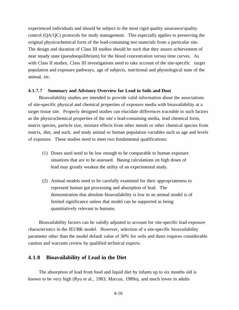
In the present case, the stress is active intestinal uptake and the displacement to undo the effect is to dissolve more lead during its passage through the gut. Such a shift, relative to a simple bench-top system, is depicted in Figures 4-5 and 4-6.

Class II Study Class II and Class III studies involve in vivo animal models of human bioavailability of

lead. They differ in their experimental specifics. Class II investigations are intermediate in vivo studies (i.e., carried out over a relatively short time). Such studies examine the bioavailability of lead within a time frame in which the dosing ends before pseudoequilibrium in the central (blood) compartment is reached. Since lead accumulates in critically important peripheral compartments such as bone and this accumulation will influence longer term uptake and distribution values, longer term studies are desirable for assessing target tissue bioavailability of lead in mammals.

Class II studies are useful in terms of providing a relative index of lead bioavailability, that is, comparison of several lead forms. Class II studies should, of course, consider all the factors already noted that influence any in vivo lead study, including the target population and pathway specifics for the site, age, concentration dependence of lead uptake in the dosing regimen, nutrition, physiology and anatomic structural characteristics.

In terms of model biology, physiology, and behavior, an appropriate selection for human simulation would take account of eating/feeding habits, human versus animal gastrointestinal tract differences, comparative biochemistry, etc.

Class III Study Bioavailability investigations that have as their purpose the site-specific adjustment of

the default bioavailability parameters in the IEUBK model may require a more complex approach. Such advanced studies should only be conducted after consultation with qualified,

4-14

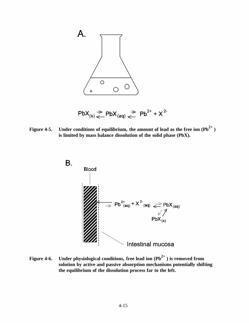
Figure 4-5. Under conditions of equilibrium, the amount of lead as the free ion (Pb2+) is limited by mass balance dissolution of the solid phase (PbX).

Figure 4-6. Under physiological conditions, free lead ion (Pb2+) is removed from solution by active and passive absorption mechanisms potentially shifting the equilibrium of the dissolution process far to the left.

4-15

experienced individuals and should be subject to the most rigid quality assurance/quality control (QA/QC) protocols for study management. This especially applies to preserving the original physicochemical form of the lead-containing test materials from a particular site. The design and duration of Class III studies should be such that they assure achievement of near steady state (pseudoequilibrium) for the blood concentration versus time curves. As with Class II studies, Class III investigations need to take account of the site-specific target population and exposure pathways, age of subjects, nutritional and physiological state of the animal, etc.

4.1.7.7 Summary and Advisory Overview for Lead in Soils and Dust Bioavailability studies are intended to provide valid information about the associations

of site-specific physical and chemical properties of exposure media with bioavailability at a target tissue site. Properly designed studies can elucidate differences traceable to such factors as the physicochemical properties of the site's lead-containing media, lead chemical form, matrix species, particle size, mixture effects from other metals or other chemical species from matrix, diet, and such, and study animal or human population variables such as age and levels of exposure. These studies need to meet two fundamental qualifications:

(1) Doses used need to be low enough to be comparable to human exposure situations that are to be assessed. Basing calculations on high doses of lead may greatly weaken the utility of an experimental study.

(2) Animal models need to be carefully examined for their appropriateness to represent human gut processing and absorption of lead. The demonstration that absolute bioavailability is low in an animal model is of limited significance unless that model can be supported as being quantitatively relevant to humans.

Bioavailability factors can be validly adjusted to account for site-specific lead exposure characteristics in the IEUBK model. However, selection of a site-specific bioavailability parameter other than the model default value of 30% for soils and dusts requires considerable caution and warrants review by qualified technical experts.

4.1.8 Bioavailability of Lead in the Diet

The absorption of lead from food and liquid diet by infants up to six months old is known to be very high (Ryu et al., 1983; Marcus, 1989a), and much lower in adults

4-16

(Chamberlain et al., 1978; Blake and Mann, 1983; Rabinowitz et al., 1980; James et al., 1985). Less is known about changes in lead absorption from diet for older infants, toddlers, and children. A value of 50% was selected as an intermediate level in children and infants (U.S. Environmental Protection Agency, 1990b).

The exact form of the dietary lead absorption coefficient in humans is not known. There is evidence that the absorption of lead in food by infants is quite high, at least 40 to 50%. The range cited by the U.S. Environmental Protection Agency (1989a) is 42 to 53%. While this probably decreases after infancy, we have no direct evidence on how to interpolate this range for children of ages 2 to 6. A smoothing of the absorption data from infant to juvenile baboon in the studies by Harley and Kneip (1985) has been proposed as a basis for extrapolation by the U.S. Environmental Protection Agency (1989a). In view of the uncertainty about this, we have chosen to keep the same default value of 50% for ages 1 to 6. This value will, at worst, slightly overestimate dietary lead uptake in older children.

Lead absorption from diet depends on the lead concentration in the stomach, and on a host of other dietary cofactors such as zinc, iron, vitamins, and phytate. When dietary lead intake during meals is sufficiently high, absorption of lead through the gut lumen decreases, probably due to competition for the limited anionic lead-binding sites on the gut wall.

The absorption of lead has some similarities with the absorption of other metals (Mushak, 1991), especially alkaline earths such as calcium and strontium. Calcium researchers have hypothesized three possible mechanisms of gut absorption. The first is a type of saturable active transport. This may be a secondary process because the enzyme requiring energy input is on the basolateral membrane and not on the membrane of the gut lumen. It would be more accurate to describe this as a facilitated diffusion process. A second saturable facilitated process involving pinocytic mechanisms has also been hypothesized by calcium researchers, but is not well understood. These saturable diffusion processes are the dominant modes of transport at low concentrations. Processes requiring carriers are often called facilitated diffusion processes. For convenience, we may call either of these saturable processes facilitated diffusion processes. The third process, the dominant mode of transport at high concentrations, is probably a simple diffusion through tight junctions on the lumenal side and is not saturable. Binding and transport of calcium across the gut lumen involves a protein called calbindin. We have described this as a passive

diffusion process. The last two processes have no specific inhibitors and are difficult to study. The extent to which lead absorption shares these calcium processes, or is quantitatively different, is not known. The study by Aungst and Fung (1981) on transport of

4-17

dissolved lead across the gut lumen in vitro in everted rat intestines shows that lead absorption is likely to consist of two distinct processes. The first process depends on a passive diffusion mechanism that is independent of gut concentration. The second process depends on a facilitated diffusion mechanism that is saturable, with a half-saturation concentration of about 120 µg/L (0.59 µmol). The quantitative extrapolation of this value to human children in vivo is uncertain.

The Glasgow duplicate diet study reported results on infant blood lead and dietary lead intake at a single time point, age 3 months. There appeared to be a very large non-dietary background source contributing about 12 µg/dL blood lead to these infants. This is attributed in part to the inhalation of leaded gasoline, which was still widely used in the United Kingdom, and in part to residual exposure pre-natally. The dietary lead intake in these infants is believed to constitute almost all of the ingested lead, since children at this young age are believed to have minimal contact with soil, house dust, or paint. Some small contribution of inhaled lead particles may be transferred to the ingestion route by mucociliary transport.

A non-linear regression model was fitted to the Sherlock and Quinn data in a form that is directly comparable to the Michaelis-Menten formula used to describe in vitro studies (Aungst and Fung 1981ab). The model that was fitted to all data was:

log(Blood lead) = log(B + L * PbIntake + K * PbIntake / (1 + PbIntake / M)).

The parameters have the following interpretation:

B = background lead concentration from pre-natal and inhalation exposure;L = linear (passive) uptake coefficient between blood lead and dietary lead intake;K = non-linear (facilitated) uptake coefficient between blood lead and dietary lead

intake; M = Michaelis-Menten type (non-linearity) parameter, the daily dietary lead intake

rate at which the facilitated component of lead uptake is half saturated.

Three methods were used to estimate the parameters. The first two methods are based on weights for the grouped data shown in Figure 4-2 of Sherlock and Quinn (1986), shown in this document as Figure 4-1. The first set of weights was based on the estimated sample size within each bar on the graph. The second method was based on the normalized coefficients of variation from the standard error bars for each group. The third method was based on

4-18

using within-cell geometric mean blood lead and dietary lead intake values from Table 4-2 in their paper, with cell counts used as weights. The first method appears to be the most accurate, both absolutely and relatively. The fitted blood lead model is:

Blood lead = 10.85 + 0.0090 PbIntake + 0.2981 PbIntake / (1 + PbIntake / 90.33)

The total blood lead to lead intake regression coefficient at low intake levels (much less than the Michaelis-Menten coefficient M = 90 µg/day) is K + L = 0.0090 + 0.2981 = 0.307 µg/dl per µg/day. The goodness of fit of this non-linear lead uptake model of Michaelis-Menten form to 3-month old human children, combined with the similar piecewise linear model that could be fitted to the water lead studies, and the goodness of fit of the Michaelis-Menten model found for the data on blood lead and lead intake data in infant and juvenile baboons presented by Mallon (1983) support the use of this model for lead absorption in older children as well. The suggestion by Chamberlain (1984) that absorption in adults is greatly reduced at intake rates above 300 µg/d is also consistent with the infant estimate of 90 µg Pb/day.

4.1.9 Bioavailability of Lead in Water

The bioavailability of dissolved lead salts in drinking water is very high when consumed by adults between meals (James et al., 1985), and very low when consumed with meals. The maximum retention of lead in children probably exceeds that of adults, which is about 60% on an empty stomach, and absorption is likely to be only somewhat smaller than retention. Thus the value of 50% is recommended as plausible. A range of values for water lead absorption from the U.S. EPA/OAQPS Staff Paper (1989a), shown in Table 4-1, should be used as a basis for age-variable absorption coefficients.

The volume of water in a typical United States faucet is about 90 to 125 milliliters, and at least two or three faucet volumes must be drawn before the tap water lead concentration decreases to the level of the source water and water distribution line lead concentrations (Schock and Neff, 1988; Gardels and Sorg, 1989; Marcus, 1991a). The sample volume of first-draw water specified in U.S. EPA's drinking water regulation is 1 L (U.S. Environmental Protection Agency, 1991c). Water lead concentrations in most U.S. water supply systems are low (<5 Fg/L), but geometric means may exceed 10 to 20 µg/L in first-draw samples from systems with highly corrosive water and a great deal of lead plumbing, which is not uncommon in older urban areas in the northeastern United States.

4-19

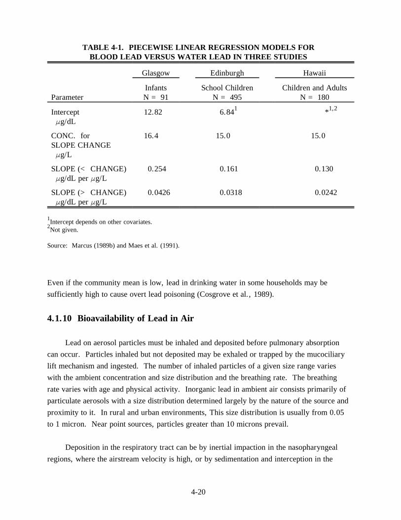
TABLE 4-1. PIECEWISE LINEAR REGRESSION MODELS FORBLOOD LEAD VERSUS WATER LEAD IN THREE STUDIES

Glasgow Edinburgh Hawaii

Infants School Children Parameter N = 91 N = 495 N = 180

Children and Adults

Intercept Fg/dL

CONC. for SLOPE CHANGE Fg/L

SLOPE (< CHANGE) Fg/dL per Fg/L

SLOPE (> CHANGE) Fg/dL per Fg/L

12.82 6.841 *1,2

16.4 15.0 15.0

0.254 0.161 0.130

0.0426 0.0318 0.0242

1Intercept depends on other covariates.2Not given.

Source: Marcus (1989b) and Maes et al. (1991).

Even if the community mean is low, lead in drinking water in some households may be sufficiently high to cause overt lead poisoning (Cosgrove et al., 1989).

4.1.10 Bioavailability of Lead in Air

Lead on aerosol particles must be inhaled and deposited before pulmonary absorption can occur. Particles inhaled but not deposited may be exhaled or trapped by the mucociliary lift mechanism and ingested. The number of inhaled particles of a given size range varies with the ambient concentration and size distribution and the breathing rate. The breathing rate varies with age and physical activity. Inorganic lead in ambient air consists primarily of particulate aerosols with a size distribution determined largely by the nature of the source and proximity to it. In rural and urban environments, This size distribution is usually from 0.05 to 1 micron. Near point sources, particles greater than 10 microns prevail.

Deposition in the respiratory tract can be by inertial impaction in the nasopharyngeal regions, where the airstream velocity is high, or by sedimentation and interception in the

4-20

tracheobronchial and alveolar regions, where the airstream velocities are lower. In the alveolar region, diffusion and electrostatic precipitation also become important.

Particles greater than 2.5 microns are deposited in the ciliated regions of the nasopharyngeal and tracheobronchial airways, where they are passed to the gastrointestinal tract by the mucociliary lift mechanism. Particles small enough to penetrate the alveolar region can be dissolved and absorbed into systemic circulation or ingested by macrophagic cells. Evidence that lead does not accumulated in the lungs suggests that lead entering the alveolar region is completely absorbed (Barry, 1975; Gross et al., 1975). Rabinowitz et al. (1977) found about 90% of the deposited lead was absorbed daily. In the IEUBK model the default assumption is that 35% of the inhaled lead is bioaccessible (reaches the absorbing surface), and 100% of this is absorbed.

4.2 USING THE INTEGRATED EXPOSURE UPTAKE BIOKINETIC MODEL FOR RISK ESTIMATION

4.2.1 Why Is Variability Important?

4.2.1.1 Intent of the Model and the Measure The Geometric Standard Deviation (GSD) as used in this manual is a measure of the

relative variability in blood lead of a child of a specified age, or children from a hypothetical population, whose lead exposures in a specified dwelling are known. The GSD is intended to

reflect the five types of individual blood lead variability identified below, not variability in blood lead concentrations where different individuals are exposed to substantially different

media concentrations of lead.

The IEUBK Lead Model is intended to be used for individual children who live at a residence, or for a hypothetical population of children who may live there in the future, or for hypothetical children who may some day live in a house built on a plot of now vacant land of appropriate size for future construction of a single residential dwelling unit.

4.2.1.2 Individual Geometric Standard Deviation Why do different children have different blood lead levels? The answer to this question

has two parts. The first part of the answer is that children are exposed to different levels of lead in their community environment. The second part of the answer is that individual

4-21

children, exposed to exactly the same measured levels of lead, will still have different blood lead levels for the following reasons:

— Different Environmental Context. Carpeting, other furnishings, and accessibility of yard soil affect contact with environmental lead in ways that are not easily measured.

— Behavioral Differences. Interaction with caretakers, with siblings and playmates, and other factors that affect mouthing behavior and play activity will modify lead intake from dust and soil.

— Different Exposures. The children will have different exposures due to differences in contact with soil, dust, water, and other environmental media that vary at different locations and different times, so that no single sample of environmental lead in any medium can be said to completely characterize the child's actual activity-weighted exposure to lead in that medium.

— Measurement Variability. The environmental lead measurements are not perfectly reproducible due to sampling location variability, repeat sampling variability, and analytical method error, so that equality of measured sample lead concentrations does not imply equality of the true exposure concentrations.

— Biological Diversity. Children are biologically diverse so that even children of the same age, weight, and height are expected to have differences in the biokinetic distribution and elimination of lead.

— Food Consumption Differences. A number of factors, including nutritional status and time of ingestion of lead relative to meal times, affect the uptake or absorption of lead ingested from a medium.

While sociodemographic factors underly many of these differences, it is not appropriate to assume any specific effect for future residents. Risk estimates should be applicable to any hypothetical resident, and this requirement adds to the variability associated with the estimate.

4-22

4.2.2 Variability Between Individuals Is Characterized by the Geometric Standard Deviation

Inter-individual variability is the starting point for risk analysis using the IEUBK model. Even if we knew the correct value for all of the environmental exposure variables, we could at best predict only the typical blood lead level expected for a child of a certain age who had that exposure. We will therefore assume that individual child blood lead levels can be divided into two parts, a predicted blood lead and a random deviation from the predicted blood lead level. A statistical model that has proven to be very useful and fits all of the blood lead studies we have analyzed is based on the following three assumptions:

(Assumption 1) Observed blood lead = (Predicted blood lead) * (Random deviation);

(Assumption 2) The random deviation is log-normally distributed with geometric mean or median = 1, and a geometric standard deviation (GSD) defined by GSD = exp (standard deviation of ln (blood lead). Here, exp(.) denotes the exponential function and ln(.) denotes the natural logarithm;

(Assumption 3) The GSD is the same for all values of the predicted blood lead (i.e., for all values of environmental exposure).

Risk is the probability of exceeding the blood lead level of concern. The IEUBK model calculates risk from these three assumptions. The user provides an exposure scenario from which the IEUBK model calculates a predicted blood lead. Then the user provides a blood lead level of concern, whose default value is now defined as 10 Fg/dL based on health effects criteria, but can be modified by the user. This risk is calculated as the probability that a standardized, normally distributed random variable exceeds the level Z, where

Z = ln (blood lead level of concern/predicted blood lead) / ln (GSD).

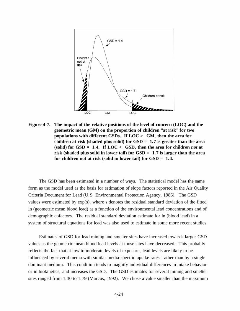
If Z = 1.645, the risk is 5%. If Z = 1.96, the risk is 2.5%. If the GSD is increased, then Z is decreased, and the risk of a blood lead level exceeding the level of concern is increased (provided that the blood lead level of concern is larger than the predicted blood lead, which is usually true). This is illustrated in Figure 4-7. The default value of Z is

Z = ln (10/predicted blood lead) / ln (1.6) = (2.3026 ! ln (predicted blood lead)) / 0.47.

4-23

LOC GM LOC

Figure 4-7. The impact of the relative positions of the level of concern (LOC) and the geometric mean (GM) on the proportion of children "at risk" for two populations with different GSDs. If LOC > GM, then the area for children at risk (shaded plus solid) for GSD = 1.7 is greater than the area (solid) for GSD = 1.4. If LOC < GSD, then the area for children not at risk (shaded plus solid in lower tail) for GSD = 1.7 is larger than the area for children not at risk (solid in lower tail) for GSD = 1.4.

The GSD has been estimated in a number of ways. The statistical model has the same form as the model used as the basis for estimation of slope factors reported in the Air Quality Criteria Document for Lead (U.S. Environmental Protection Agency, 1986). The GSD values were estimated by exp(s), where s denotes the residual standard deviation of the fitted ln (geometric mean blood lead) as a function of the environmental lead concentrations and of demographic cofactors. The residual standard deviation estimate for ln (blood lead) in a system of structural equations for lead was also used to estimate in some more recent studies.

Estimates of GSD for lead mining and smelter sites have increased towards larger GSD values as the geometric mean blood lead levels at those sites have decreased. This probably reflects the fact that at low to moderate levels of exposure, lead levels are likely to be influenced by several media with similar media-specific uptake rates, rather than by a single dominant medium. This condition tends to magnify individual differences in intake behavior or in biokinetics, and increases the GSD. The GSD estimates for several mining and smelter sites ranged from 1.30 to 1.79 (Marcus, 1992). We chose a value smaller than the maximum

4-24

that is consistent with the remaining variability after differences in the usual site specific soil lead and dust lead measurements have been removed. The remaining sources of variability include not only biological and behavioral variability in the children, but also repeat sampling variability, sample location variability, and analytical error. For empirical support in selecting a site specific GSD see Appendix A.

The default value is:

GSD = 1.6.

This default value is based on calculations of GSDs from specific sites. The median GSDs weighted for sample size within cells were estimated as 1.69 for Midvale, 1.53 for the Baltimore data of the Urban Soil Lead Abatement Demonstration Project, and 1.60 for the Butte study. This type of adjusted GSD calculation was chosen because of its treatment of outliers. Other types of adjusted GSDs, such as those derived from structural analyses are described below.

We must discourage the user from changing the GSD value by use of empirical site-specific data from a blood lead study. As discussed in Section 4.5 below, blood lead studies may be subject to subtle sampling biases and changes in child behavior in response to the study. The GSD value reflects child behavior and biokinetic variability. Unless there are great differences in child behavior and lead biokinetics among different sites, the GSD values should be similar at all sites, and site-specific GSD values should not be needed.

The user may wish to demonstrate that the variability in a specific well-conducted blood-lead study is consistent with the default assumption. In the next section, we will describe how to estimate a site-specific, inter-individual GSD when necessary. These analyses should be done only when necessary, and with thorough documentation of the reasons why the site may have more or less variation among child behavioral and biological parameters than at most other sites. We must remind the user that it is not necessary to have

site-specific blood lead data in order to appropriately use the model with the default GSD.

4.2.3 Statistical Methods for Estimating the Geometric Standard Deviation from Blood Lead Studies

We have used several statistical methods to estimate GSD values recommended here. Two methods are described in detail in Appendix A. The first method is a direct method in

4-25

which environmental lead levels are fixed in ranges or intervals, and blood lead variability for children exposed to these concentrations is calculated directly. The second method is a statistical regression method appropriate to the generally skewed distribution of blood lead values and estimates the variability in blood lead concentrations after an empirical estimate of blood lead concentrations expected at each environmental lead concentration. The two methods give reasonably consistent results. The regression method uses child-specific age and lead concentration. The regression method crudely mimics the IEUBK model.

4.2.4 Choosing the Geometric Standard Deviation: Intra-Neighborhood Variability

There have been some cases in which the IEUBK Lead Model or a preceeding model was used to estimate the distribution of blood lead in a community when only community-level input was available, such as geometric mean soil, dust, and air lead. Further experience with the IEUBK model suggests that this application may be appropriate under some conditions in which certain mathematical assumptions are approximately correct. It also suggests that there are some other situations in which this approach is incorrect because the necessary mathematical assumptions are not satisfied. At this time, we recommend using the IEUBK Lead Model for neighborhood and individual blood lead assessment, but not for communities or for larger scale blood lead assessments without carefully evaluating the input assumptions. The neighborhood scale assessment requires stratifying the neighborhood by intervals of soil and dust lead.

A neighborhood is a spatially contiguous area that often has identifiable physical or geographical boundaries. For the purposes of this manual, a neighborhood is characterized according to the following guidelines:

• Boundaries such as a highway, railroad right-of-way, river, or by non-residential land uses such as commercial, industrial, agricultural, or park;

• Approximately 400 households with about 100 children;

• Church, school, and retail establishments within walking distances;

• Diameter about 1.5 kilometers (1 mile).

4-26

The neighborhood concept is used here to classify small areas of relatively similar childhood lead exposure, and will rarely be the same as a census tract, political locale such as a precinct or ward, or community association membership area.

Input parameters for the model at a neighborhood scale should be some measure that characterizes typical exposure concentration in a medium, such as the arithmetic mean or geometric mean, or the median. When activity pattern or behavior weighted exposure information is unavailable, we recommend use of the arithmetic mean to characterize soil lead concentrations in areas that are sufficiently small that any part of the area may be accessible to a typical child living at a random residence located within the area. This will certainly be applicable to the yard and adjacent play areas of a single residence.

Our recommended approach for risk estimation involves more calculations than the single-input soil and dust lead, but much less calculation than the use of each individual yard or housing unit. Our approach requires the division of the neighborhood into units that are larger than single yards or other sites, but smaller than the whole neighborhood, and clearly must depend on the scale of a risk assessment. Risk within a neighborhood can be assessed in a single model run only if media concentrations of lead are relatively homogeneous between different residential sites.

There is no definition of a "community" for model use. It is expected that older children will be able to play anywhere within a neighborhood, but are limited to their own neighborhood within the community. An alternative approach is to define "neighborhoods" by isopleths or contours of soil lead concentrations, but this is more likely to be useful in the vicinity of active or inactive smelter or battery recycling plants, where soil lead deposition has a definite point source pattern. No specific approach based on Geographic Information Systems (GIS) data bases has yet been adopted. The definition of neighborhood scale suggested here is roughly equivalent to an area of 4 to 10 city blocks in many urban areas (160 to 240 meters square). A neighborhood should not be larger than a one kilometer square.

4.2.5 Basis for Neighborhood Scale Risk Estimation

The basis of the neighborhood approach is that a few important environmental parameters largely determine the predicted geometric mean blood lead. Since the environmental lead concentrations are known to have some measurement error, there should be little loss of accuracy in grouping the environmental lead concentrations by small

4-27

intervals. For example, the interval ranges for soil lead concentration could be 0 to 249 Fg/g, 250 to 499 Fg/g, 500 to 749 Fg/g, etc. Soil lead levels in an interval, for example from 250 to 499 Fg/g, would be described by a single number in that range, such as the midpoint of the interval at 375 Fg/g.

One of the most important determinants of blood lead concentration in children is lead in household dust. It is necessary to use small intervals of dust lead concentration along with small intervals of soil lead concentration. There are many other sources of lead in household dust in addition to soil lead, including dust lead from air lead deposition, from interior lead-based paint, and from workplace dust carried home by adults residing in the house. The actual range of dust lead concentrations corresponding to a soil lead interval is therefore generally much wider than the range of soil lead concentrations.

There may be circumstances in which other lead exposures in a neighborhood are known, and vary over a wide range. For example, there may be information on water lead concentrations in different houses. Some of the houses may have sufficiently high water lead concentrations that lead in water becomes another significant source of lead exposure. Additional stratification or classification of sites by this variable may also be useful.

Neighborhoods defined by small geographic areas are also much more likely to be homogeneous with respect to sociodemographic factors that affect blood lead variability. There should be some similarity in child activity patterns, household environmental contexts, behavioral patterns, and nutritional patterns within a neighborhood. Therefore, the individual GSD may be applied plausibly to the relatively homogeneous subpopulation within a neighborhood. If the neighborhood defined initially is very heterogeneous, then a larger GSD may be needed. It would be better to subdivide the neighborhood defined initially into more homogeneous subareas. This requires knowledge about the neighborhood residents, or an assumption about future residents.

4.2.6 Relationship Between Geometric Standard Deviation and Risk Estimation

The GSD is a very sensitive parameter for risk estimation. In this model, we use "risk" in the following specific ways:

4-28

• Individual risk is the probability that a hypothetical child living in a particular house or dwelling unit characterized by its environmental lead levels will have a blood lead concentration that exceeds a user-specified level of concern;

• Neighborhood or community risk is the fraction of children in a neighborhood or community characterized by a specified distribution of environmental lead concentrations that are expected to have blood lead concentrations exceeding a user-specified level of concern.

The assessment of potential health risk from environmental exposure to toxicants is one of EPA's most significant activities. We are using only part of this process. An elevated blood lead concentration (however one defines "elevated") is an index of internal exposure or body burden of lead. It is a useful index precisely because it changes in response to changes in exposure, with characteristic time scales of a few days or so in plasma and red blood cells, reflecting deeper changes of a few months in soft tissues, and years in hard bone. An elevated blood lead concentration is not precisely an adverse health effect by itself, but has been a very useful predictor of an increased likelihood of neurobehavioral deficits in children. The "risk" involved here is the risk of an increase in an easily measured index of lead exposure that is a predictor of adverse health effects.

The most general form of the model is multiplicative:

Blood lead = controllable factors * random factors.

For a single child, with defined sources of exposure, the IEUBK model estimates the geometric mean blood lead, or typical blood lead (i.e., the median when variability is log-normal, as it usually is). The model then is given by:

Blood lead = GM * exp( Z * ln(GSD) )

where GM is the model-predicted geometric mean blood lead, exp(.) is the exponential function, ln(.) is the natural logarithm function, and Z is a normally distributed random variable. Therefore risk, defined as a probability for a single child, is calculated by the equation

Risk = Probability{Blood lead > level of concern for given exposure}

4-29

= Probability{Z > (ln(level of concern) - ln(GM)) / ln(GSD)}.

When the level of concern is greater than the expected or typical blood lead at that exposure, then risk increases when GSD increases. Figure 4-7 illustrates the difference in "at risk" children for two populations, one with a GSD of 1.4 and another with 1.7. When the level of concern is above the geometric mean, the population with the higher GSD has a greater proportion of the children at risk. When the level of concern is less than geometric mean, the population with the lower GSD has a greater proportion of children at risk.

4.2.7 Risk Estimation at a Neighborhood or Community Scale

4.2.7.1 What Do We Mean by "Neighborhood" or "Community" Risk? Representative questions of interest in assessing the risk of elevated child blood lead in

a neighborhood are:

• What is the frequency distribution of risk of exceeding a blood lead concentration of concern, such as 10 Fg/dL, within the neighborhood?

• What fraction of a hypothetical or actual population of children would be expected to exceed some specified blood lead concentration of concern if they resided in the representative sample of houses in this neighborhood for which we have soil and dust lead data?

• How much could we reduce high individual risk or the fraction of children with elevated blood lead concentrations by cleaning up soil to some specified level?

• What is the distribution of risks for a hypothetical population of children if housing units were constructed on soil at this vacant site?

The implicit definition of risk in these questions is the fraction of children living in a dwelling unit anywhere in the neighborhood who have elevated blood lead levels. We see that the neighborhood or community risk level has two distinct components of variability:

(1) Inter-individual differences, as in Section 4.2.4; and (2) Inter-dwelling unit differences in lead exposure.

4-30

In some circumstances, these two can be combined and the same approach used to estimate the fraction of children at risk in a neighborhood. But, if there is a broad distribution of inter-dwelling unit differences, as is commonly observed, then a simplistic application of the IEUBK model may substantially under-estimate the real risk from the most contaminated parts of the neighborhood. Whatever the distribution of inter-dwelling unit or intra-neighborhood exposure levels, the "sum of risks" approach can always be applied. Note that there is a subtle difference between inter-dwelling exposure and intra-neighborhood exposure. Inter-dwelling exposure distribution would be the distribution of exposures measured in each home and would assume that the individual exposure is within the property boundaries of the dwelling unit. Intra-neighborhood exposure would include additional exposure from nonproperty sources, such as parks, schools and playgrounds.

4.2.7.2 Neighborhood Risk Estimation as the Sum of Individual Risks Neighborhood risk is based on the expected number of children in the neighborhood

who have elevated blood lead levels, here taken as greater than 10 Fg/dL. Using the computer model, some of these questions can be addressed by the following procedure:

1. Set up a batch mode file in which each line represents the age and environmental lead exposure of each child in the real or hypothetical population.

2. Use the IEUBK Lead Model to estimate the geometric mean blood lead for each child in the batch mode file.

3. Apply an individual GSD to estimate the probability of exceeding the blood lead level of concern for each child or each household in the batch mode file.

4. Calculate the expected number of blood lead values exceeding the level of concern by adding up the probability of exceeding the blood lead level of concern across all children in the batch mode file.

Note that even houses with low lead concentrations have a small positive risk for resident children. In houses with high lead concentrations, the risk of elevated blood lead is much larger, but some children (even in those high lead houses) will not have elevated blood lead concentrations. The total of all such risks characterizes neighborhood exposure.

4-31

5. Neighborhood risk is the ratio of the calculated expected number of blood lead values exceeding the level of concern to the total number of children in the batch mode file. This last point is illustrated in the following narrative.

4.2.7.3 An Example for the "Sum of Individual Risks" Approach Suppose that there are data on four households with children in a neighborhood.

Residents of each household are exposed to lead-contaminated soil. The first house has 250 Fg/g lead in soil, the second has 250 Fg/g, the third has 1000 Fg/g, and the fourth house has 1000 Fg/g. We have assumed dust lead concentrations as 70 percent of the soil lead concentration in houses 2 and 4, and as 15 percent of the soil lead concentration in houses 1 and 3. We have added 10 Fg/g to dust lead as an estimate of the air lead contribution to dust lead at 0.1 Fg Pb per cubic meter of air. The respective dust lead concentrations are thus 47.5 Fg/g, 185 Fg/g, 160 Fg/g, and 710 Fg/g.

The neighborhood is usually not just 4 houses. We may have samples at only these 4 houses, or there may be 100 houses at each of these 4 soil and dust lead concentrations. The assumption is that the samples are representative of the exposure distribution in the neighborhood. We are showing calculations for four houses only for the purposes of illustration. The risk estimates are intended to be unbiased estimates of potential risk for other years in which different children, not in the current sample, may occupy the same or other houses in the neighborhood. Obviously, a reliable estimate of neighborhood risk will require many more than 4 houses.

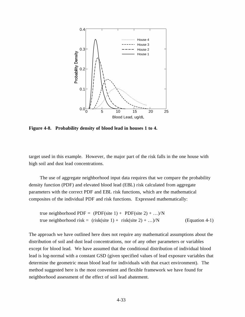
All other parameters are set to default values. We used a soil and dust absorption model with 30% absorption of lead from both dust and soil. (Smaller values of soil lead absorption may be needed for some sites—see Section 4.1). We assumed GSD = 1.6; larger values of GSD may be needed at some sites. The probability density of blood lead for four houses is shown in Figure 4-8.

For the house with soil lead at 250 Fg/g and dust lead at 47.5 Fg/g, we expect 0.55% of children to exceed 10 Fg/dL. For the house with 250 Fg/g soil lead and 185 Fg/g dust lead, we expect 1.99% to exceed 10 Fg/dL. For the house with soil lead at 1,000 Fg/g and dust lead at 160 Fg/g, we expect 21.06% of children to exceed 10 Fg/dL. For the house with 1000 Fg/g soil lead and 710 Fg/g dust lead, we expect 42.68% to exceed 10 Fg/dL. The sum of the risks for these four houses is 0.55% + 1.99% + 21.06% +42.68% = 66.28% children = 0.6628 children expected to exceed 10 Fg/dL, or an average risk for the neighborhood of 66.28% / 4 = 16.57%, which is greater than the 5% neighborhood risk

4-32

0.4

0.3

House 4

House 3

House 2 House 1

0.2

0.1

0.00 5 10 15 20 25

Blood Lead, ug/dL

Figure 4-8. Probability density of blood lead in houses 1 to 4.

target used in this example. However, the major part of the risk falls in the one house with high soil and dust lead concentrations.

The use of aggregate neighborhood input data requires that we compare the probability density function (PDF) and elevated blood lead (EBL) risk calculated from aggregate parameters with the correct PDF and EBL risk functions, which are the mathematical composites of the individual PDF and risk functions. Expressed mathematically:

true neighborhood PDF = (PDF(site 1) + PDF(site 2) +...)/N

true neighborhood risk = (risk(site 1) + risk(site 2) +...)/N (Equation 4-1)

The approach we have outlined here does not require any mathematical assumptions about the distribution of soil and dust lead concentrations, nor of any other parameters or variables except for blood lead. We have assumed that the conditional distribution of individual blood lead is log-normal with a constant GSD (given specified values of lead exposure variables that determine the geometric mean blood lead for individuals with that exact environment). The method suggested here is the most convenient and flexible framework we have found for neighborhood assessment of the effect of soil lead abatement.

4-33

4.2.7.4 Assessment of Risk Using Grouped Data for a Neighborhood The example in the preceding section had a "neighborhood" with only 4 houses, so that

the amount of work required was not very burdensome. In the real world, the site manager or risk assessor may be dealing with relatively homogeneous neighborhoods or small communities with several hundred households. These calculations can be simplified by grouping soil and dust lead levels into small cells with fixed ranges of values. The grouped data within each cell are all assigned the same value, such as the midpoint of the interval.

Each cell is then assigned a statistical weight. The statistical weights could be:

(1) The number of housing units with soil and dust lead concentrations in the interval;

(2) The number of children observed or expected to live in housing units with soil and dust lead concentrations in the interval;

(3) The fraction of housing in a neighborhood that is expected to have soil and dust lead concentrations in the interval;

(4) The fraction of area in as-yet-undeveloped neighborhoods with soil and dust lead concentrations in the interval.

The probability density function (PDF) and risk of EBL children in then the weighted sum of the cell PDF or cell risks. If the respective weights are denoted weight (cell 1), weight (cell 2), etc., and the PDFs are denoted PDF (cell 1), PDF (cell 2), etc., and the risks are denoted risk (cell 1), risk (cell 2), etc., then:

neighborhood PDF = [weight (cell 1) * PDF (cell 1) + weight (cell 2) * PDF (cell 2) + etc.] / [weight (cell 1) + weight (cell 2) + etc.]

neighborhood risk = [weight (cell 1) * risk (cell 1) + weight call (cell 2) * risk (cell 2) + ...] / [weight (cell 1) + weight (cell 2) + ...]

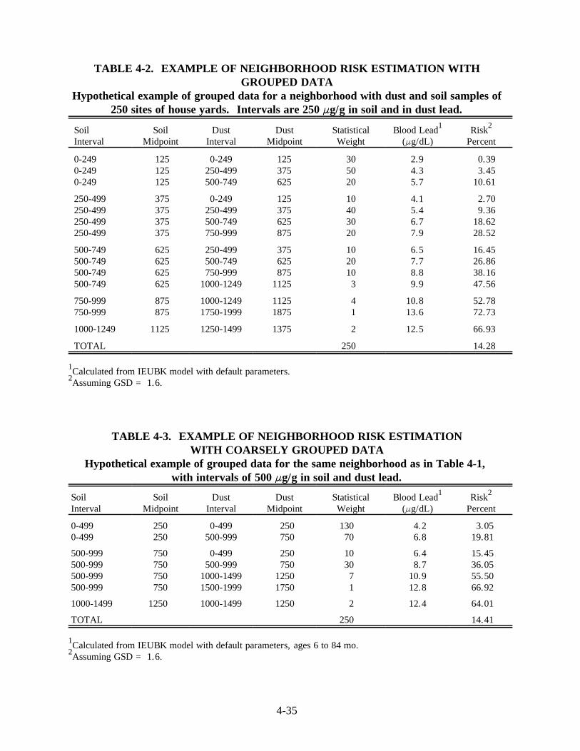
The following hypothetical example may illustrate these points. Suppose that a random sample of 250 houses and apartments has been obtained in a neighborhood. The number of houses in each interval of 250 Fg/g soil and 250 Fg/g dust lead is shown in Table 4-2. This

4-34

F

F

TABLE 4-2. EXAMPLE OF NEIGHBORHOOD RISK ESTIMATION WITHGROUPED DATA

Hypothetical example of grouped data for a neighborhood with dust and soil samples of250 sites of house yards. Intervals are 250 Fg/g in soil and in dust lead.

Soil Soil Dust Dust Statistical Blood Lead1 Risk2

Interval Midpoint Interval Midpoint Weight (Fg/dL) Percent

0-2490-2490-249

125125125

0-249250-499500-749

125375625

305020

2.94.35.7

0.39 3.45

10.61

250-499 375 0-249 125 10 4.1 2.70 250-499 375 250-499 375 40 5.4 9.36 250-499 375 500-749 625 30 6.7 18.62 250-499 375 750-999 875 20 7.9 28.52

500-749 625 250-499 375 10 6.5 16.45 500-749 625 500-749 625 20 7.7 26.86 500-749 625 750-999 875 10 8.8 38.16 500-749 625 1000-1249 1125 3 9.9 47.56

750-999750-999

875875

1000-12491750-1999

11251875

41

10.813.6

52.7872.73

1000-1249 1125 1250-1499 1375 2 12.5 66.93

TOTAL 250 14.28

1Calculated from IEUBK model with default parameters.2Assuming GSD = 1.6.

TABLE 4-3. EXAMPLE OF NEIGHBORHOOD RISK ESTIMATIONWITH COARSELY GROUPED DATA

Hypothetical example of grouped data for the same neighborhood as in Table 4-1, with intervals of 500 Fg/g in soil and dust lead.

Soil Soil Dust Dust Statistical Blood Lead1 Risk2

Interval Midpoint Interval Midpoint Weight (Fg/dL) Percent

0-4990-499

250250

0-499500-999

250750

130 70

4.26.8

3.05 19.81

500-999 750 0-499 250 10 6.4 15.45 500-999 750 500-999 750 30 8.7 36.05 500-999 750 1000-1499 1250 7 10.9 55.50 500-999 750 1500-1999 1750 1 12.8 66.92

1000-1499 1250 1000-1499 1250 2 12.4 64.01

TOTAL 250 14.41

1Calculated from IEUBK model with default parameters, ages 6 to 84 mo.2Assuming GSD = 1.6.

4-35

same example is shown in Table 4-3 in intervals of 500 Fg/g in soil and 500 Fg/g in dust. There is no requirement that there be equal interval lengths in either soil or dust.

The user may then calculate neighborhood risk in three ways:

• Sum of risks for 250 housing units;

• Sum of risks for 14 cells or groups of width 250 Fg/g soil and dust;

• Sum of risks for 7 cells or groups of width 500 Fg/g in soil and dust.

The results of calculations are shown in the Tables 4-2 and 4-3. The total risk in Table 4-3 is

calculated as:

(130 * 3.05% + 70 * 19.81% + 10 * 15.45% + 30 * 36.05% +

7 * 55.50% + 1 * 66.92% + 2 * 64.01%)/250 = 14.41%

The risk calculation in Table 4-2 is similar. If there are not too many cells, the amount of

calculation can be strikingly reduced. However, as the intervals are made longer, there is a

corresponding loss of accuracy in the neighborhood risk estimate. The extra effort in

calculating risks with 250 Fg/g intervals (14 cells) is probably compensated by the increased

precision, with an estimate of 14.28% instead of 14.41%. The actual risk for the ungrouped

sample with 250 simulated houses in 14.13%.

4.2.7.5 Assessment of Risk with Neighborhood or Neighborhood-Scale Input

There are situations in which it is either inconvenient or impossible to apply the IEUBK

model at the intended household residence scale. For example, if only neighborhood mean

values or geometric mean values of input parameters such as soil and dust lead are available,

the model estimate may be far less reliable than if individual residential measurements were

made. Another possibility is that there are a substantial number of soil and dust lead

measurements at a site, but not at houses or locations within the site where blood lead and

EBL risk estimates are needed, for example, to compare with blood leads observed at

residences where there are no environmental data. There are some circumstances in which

this is clearly not a valid application of the model. As we do not clearly understand the range

of conditions under which the IEUBK model may be used with large-scale input data at this

time, we must discourage use of the IEUBK model except with single-residence or residential

lot-sized input data, or with data grouped into cells as in Section 4.2.7.4.

4-36

4.3 ENVIRONMENTAL PATHWAY ANALYSIS

4.3.1 Concept of Pathway Analysis

Environmental pathways for lead have been a subject of interest for EPA for a long

time. Methods for analyzing with multi-media exposure pathways from air lead were used in

developing slope factors for blood lead versus air lead, dust lead, and soil lead in EPA's Air

Quality Criteria document (U.S. Environmental Protection Agency, 1986). Even though the

focus was on exposure to air lead as a primary source, it was clearly recognized that

whatever the source of lead in air, paint, or soil, the primary exposure vector for young

children was through fine particles of surface soil and household dust that adhered to the

children's fingers and were ingested in the course of normal hand-to-mouth contact at ages

one to five years. Thus the total impact of air lead exposure had to be evaluated as the sum

of exposure over several pathways (Figure 4-9).

Au to Em issions

Industrial Em issions

C rustal Wea thering

Amb ient A ir So il Su rface and

G round Water

Pa int, Industrial

Dusts P lants An imals

So lder Lead G lazes

Inhaled A ir Dusts Food Drinking

Water

Ch ild

Figure 4-9. Exposure pathways of lead in the environment.

4-37

The IEUBK model assists the user in defining critical pathways for each exposure scenario. For example, there are two places on the Multiple Source Analysis Menu for household dust where pathway information may be inserted:

(1) the soil-to-to-dust pathway coefficient may be entered in the first line of the Multiple Source Analysis Data Entry Menu, replacing the default value of 0.70 µg/g dust per µg/g soil lead;

(2) the direct air-to-dust pathway coefficient is on the second line of the Multiple Source Analysis Data Entry Menu, replacing the default value of 100 µg/g dust lead per µg/m3 air Pb.

The following paragraphs provide the basis for some of the default parameters used in the IEUBK model, and suggest some methods for estimating alternate coefficients from site-specific data, provided the user has some knowledge of statistical regression. While physical measurement methods such as a comparison of stable lead isotope composition ratios have been used for source apportionment studies (Yaffee et al. 1983; Rabinowitz 1987), most users will probably have to infer site-specific pathway parameters by statistical analyses of field data.

4.3.2 Pathway Analyses by Linear Regression

The slope factor approach, described in Section 1.5, determines the linear relationship between two pathway components. This methods was used for the EPA Exposure Analysis Methodology Validation (U.S. Environmental Protection Agency, 1989a) to show that there is a clear relationship between lead in air (PbA), lead in soil (PbS), and lead in dust (PbD). This relationship may be approximately linear, depending on properties of soil and dust lead particles; if not linear, then it is at least a positive cause and effect relationship. The relationship was established using data from air lead point sources such as primary and secondary lead smelters, other non-ferrous metal smelters, and lead battery plants. The analysis, using mean values, found the relationship:

PbD = bD0 + bDA PbA + bDS PbS (Equation 4.3-2)

where bDS = 0.364 for all point source communities, but = 0.894 for the East Helena primary lead smelter community. This suggests that there may be substantial differences among communities in terms of soil-to-dust transfer.

4-38

The direct air-to-soil relationship was also estimated:

PbS = bS0 + bSA PbA (Equation 4.3-3)

When estimating slope factors by a sequence of regression equations the user should be aware that the "measurement errors" in pathway equations will almost certainly attenuate the size of the regression coefficients, and could even reverse the sign of the coefficients (Kupper 1984). Structural equation modeling techniques attempt to resolve this problem by the simultaneous estimation of coefficients in pathway models in the face of measurement errors.

4.3.3 Pathway Analysis Using Structural Equation Models

Systems of linear equations in which the output of one equation (such as PbD predicted from PbS and XRFI) is used as the input or predictor in another equation (such as PbB from PbD) can be reliably estimated using a method known as structural equation models (Bollen 1990). This method was introduced in the analysis of blood lead data by Bornschein et al. (1985) and Clark et al. (1985) in their analyses of data from the Cincinnati Prospective Childhood Lead Study. Several authors have extensively explored applications of the method to environmental lead data (Marcus 1991; Burgoon and Menten 1991). Two different approaches were compared, and found to produce very similar results.

The first approach uses linear equations without logarithmic transformation, but with a robust method of estimation that is not sensitive to skewness or to instability of measurement error variances. (The software implementation in the EQS program (Bentler 1989) was particularly convenient.) For a lead mining community, or an urban area in which air lead levels are so low as to be negligible predictors of blood lead, A typical small system of equations might be:

PbB = bB0 + bBS PbS + bBD PbD + bBXI XRFI (Equation 4.3-6)

PbD = bD0 + bDXI XRFI + bDS PbS (Equation 4.3-7)

PbS = bS0 + bSXE XRFE + bSage House-age (Equation 4.3-8)

where: PbB = blood lead concentration (Fg/dL)

4-39

PbS = soil lead concentration (Fg/g)PbD = dust lead concentration (Fg/g)XRFI = interior measurement of lead-based paint by XRF (mg/cm2)XRFE = exterior measurement of lead-based paint by XRF (mg/cm2)bnm = raw regression coefficient where the subscript refers

to: response variable n on predictor m,B0 = interceptBD = blood to dustBXI = blood to XRFID0 = interceptDXI = dust to XRF (interior)DS = dust to soilS0 = interceptBS = blood to soilSXE = soil to XRF (exterior)Sage = soil to house age

This model assumes that there is direct ingestion of interior lead paint, which also contributes to household dust, but no direct ingestion of exterior lead-based paint. The exterior lead-based paint contribution is subsumed in the paint to soil to dust pathway. Because of the linear equation formulation, partial effects of lead source terms are preserved:

PbB = cB0 + cBS PbS + cBXI XRFI

PbB = dB0 + dBXE XRFE + dBXI XRFI

cBS = bBS + bBD bDS

dBXI = bBXI + bBD bDXI

dBXE = (bBS + bBD bDS) bSXE

(Equation 4.3-9)

(Equation 4.3-10)

(Equation 4.3-11)

(Equation 4.3-12)

(Equation 4.3-13)

where: cBm = composite regression coefficient for blood on predictor m dnm = composite regression coefficient for indirect pathways from predictor m

to response n

4-40

The second approach uses logarithmic transformation of the equations in the system Equations 4.3-6 through 4.3-8:

log(PbB) = log(bB0 + bBS PbS + bBD PbD + bBXI XRFI)(Equation 4.3-14)

log(PbD) = log(bD0 + bDXI XRFI + bDS PbS) (Equation 4.3-15)

log(PbS) = log(bS0 + bSXE XRFE + bSage House-age) (Equation 4.3-16)

This system can be estimated using SAS PROC MODEL or similar programs for non-linear systems modelling. All of the coefficients were constrained to be non-negative, since negative coefficients are non-interpretable. However, the appearance of a negative estimate for an intrinsically positive coefficient should be taken as a diagnosis of some statistical problem, such as multi-colinearity or the omission of important predictive variables.

4.3.4 Regression Analyses for Multiple Exposure Pathways: Soil Example

The variables for regression analyses were described briefly in Section 1.5. The use of a regression coefficient in risk assessment is a complicated matter, because one can use either aggregate regression coefficients, which combine information on all exposure pathways, or disaggregate regression coefficients in which each exposure pathway has its own slope coefficient. The exposure of young children to air lead includes soil and dust pathways, as well as direct inhalation. This is discussed in detail in the OAQPS staff papers (U.S. Environmental Protection Agency, 1989ab) based on earlier work by Brunekreef (1984). The aggregate blood lead regression coefficient for air lead, including soil and dust exposure pathways, is cBA = 5 to 6 µg Pb/dL blood per µg Pb/m3 air, whereas the direct inhalation coefficient bBA is only about 2 µg Pb/dL blood per µg Pb/m3 air. For a simple soil lead pathway model,

soil ÿ dust ÿ hands ÿ child soil ÿ hands ÿ child

whose equations are given by

PbB = bB0 + bBS PbS + bBD PbD (Equation 4.3-17)

PbD = bD0 + bDS PbS (Equation 4.3-18)

4-41

the aggregate blood lead vs. soil lead regression coefficient should be

cBS = bBS + bBD bDS (Equation 4.3-19)

An empirical regression coefficient approach would use only the three coefficients bBS, bBD and bDS. In the absence of data from a well-conducted child blood lead study at the same site or at some similar site, including both soil and dust lead data matched to each child's total lead exposure, there is no basis for calculating the aggregate soil lead coefficient. However, the use of a model like the IEUBK model allows estimation of the parameters bBS and bBD in Equation 4.3-8 from a synthesis of many diverse studies and does not require blood lead data at the site. Any additional information about site-specific exposure and soil or dust lead characteristics would progressively refine the model predictions, even without a child blood lead study. Site-specific soil and dust lead data are needed in either approach. The IEUBK model has a parameter in the Multiple Source Analysis for Dust in which the soil-to-dust coefficient bDS can be inserted.

4.4 USE OF DATA FROM BLOOD LEAD STUDIES

4.4.1 Overview

In general, data from well-conducted blood lead studies of children at a site can provide useful information to the risk assessor and site decision maker. The purposes of this chapter are to explain what type of information a well-conducted blood lead study can provide, how blood lead study data can be used when assessing exposure to lead, and how to interpret model predictions when blood lead data for a site are also available.

Proper design and conduct of a blood lead study are critical if the results of the study are to be considered by the risk assessor. Blood lead data alone, without environmental lead exposure data and without elements of study design that control rapid changes in exposure prior to sampling, or without adequate control for sampling and analysis, should not be used to assess risk from lead exposure or to develop soil lead cleanup levels. However, a well-designed and conducted blood lead study can be useful in conjunction with site-specific environmental data in evaluating risk to children.

Blood lead concentrations are widely held to be the most convenient, if imperfect, index of both lead exposure and relative risk for various adverse health effects (U.S. Environmental

4-42

Protection Agency, 1986). In terms of exposure, however, it is generally accepted that blood lead concentrations yield an index of relatively recent exposure because of the rather rapid clearance of absorbed lead from the blood. Such a measure, then is of limited usefulness in cases where exposure is variable or intermittent over time, as is often the case with pediatric lead exposure.

According to the EPA Science Advisory Board in its 1992 report, "Review of the Uptake Biokinetic Model for Lead" (U.S. Environmental Protection Agency, 1992a), blood lead concentrations are responsive to abrupt or unanticipated changes in recent lead exposure for children. Since internal exposure is a function of lead intake (concentration multiplied by intake rates) and uptake, these changes can be environmental, behavioral, and physiological. For example, leaving a child in a house where lead-based paint has just been sanded would likely result in a significant elevation in that child's blood lead concentration. Reduction in a child's blood lead concentration may result from altered behavior that reduces exposure to lead (i.e., more frequent house cleaning, more attention to child's cleanliness, etc.). Cross-sectional blood lead studies (all done within a short time interval) are most useful when there is no reason to believe that child lead exposure has changed significantly within the last few months due to changes in environment or behavior.

A blood lead value may say little about any excessive lead intake at an early age, even though early childhood exposure may have resulted in significant irreversible toxicity. On the other hand, analyses that are retrospective in nature such as whole tooth or dentine analyses can only be done after the particularly vulnerable age in children—under 4-5 years— has passed. Such a measure, then, provides little basis upon which to implement regulatory policy for environmental or clinical intervention.

Furthermore, over a relatively broad range of lead exposure through some medium, the relationship of lead in the external medium to lead in blood is curvilinear, such that relative change in blood lead per unit change in exposure level generally becomes increasingly less as exposure increases. This behavior may reflect changes in tissue lead kinetics, reduced lead absorption, or increased excretion. In any event, modest changes in blood lead concentrations with exposure at the higher end of this range are in no way to be taken as reflecting correspondingly modest changes in body or tissue uptake of lead, (U.S. Environmental Protection Agency, 1986).

Data from good quality blood lead studies can be useful in examining the predictiveness of the model. The IEUBK Model predicts blood lead concentrations in children younger than

4-43

84 months based on environmental inputs for soil, house dust, water, air, and dietary lead intake. It would be logical to assume that the distribution of blood lead concentrations predicted by the model using site-specific data would be generally similar to those measured in the population, provided that the actual blood lead study was well designed and conducted. The IEUBK Model may not be able to account for all sources of exposure. If the predicted blood lead concentrations are not similar to those observed, an attempt should be made to identify the reasons for those differences.

It is important to recognize that most implementations of the lead model now rely on the assumption that exposure to lead in soil and dust is primarily residential in nature. However, in an actual population of children, there will be substantial opportunity for non-residential lead exposures. Periods of time spent away from the home may also have the effect of reducing the residential exposures that would otherwise occur. The fact that the model applications cannot now track all aspects of nonresidential of lead sources that a child may encounter implies that a precise match between calculated and predicted blood lead distributions cannot be expected. Nevertheless, due to the importance of residential exposures to lead in children, a reasonable overall agreement should be anticipated in such comparisons. These considerations argue that reliance on P-values from statistical tests is not an appropriate basis for judging the comparability between observed and predicted blood lead concentrations. It should be noted that calculations of blood lead concentrations on the assumption of residential exposure is a useful endpoint in site risk evaluation, as many children will indeed experience primarily residential exposures to lead.

It is important to understand that the model should not necessarily be expected to reproduce the observed blood lead concentrations exactly. The model predicts the geometric mean blood lead level corresponding to a given set of exposure inputs. Probability distribution estimates produced by the model for a given GSD can be used to define a prediction interval for blood lead concentrations. As long as the interval includes the observed blood lead corresponding to the same exposure inputs, the model has performed adequately. Even when a predicted blood lead interval for a set of exposure inputs does not overlap an observed blood lead level, there may be plausible explanations owing to the complex nature of multi-media exposures and the difficulty in characterizing all the relevant determinants of these exposures, and the degree of inter-individual variation in blood lead concentrations that is known to exist even when exposure is very well characterized.

4-44

4.4.2 Data Quality

The quality of blood lead data can be specified by Data Quality Objectives (DQOs) which are established prior to the data collection effort. This DQO effort, as outlined in the Guidance for Data Useability in Risk Assessment, Part A (U.S. Environmental Protection Agency, 1992b), should result in a sampling and analysis plan which details the chosen sampling and analysis options, and provides goals for confidence intervals. The data quality indicators of completeness, comparability, representativeness, precision, and accuracy can provide quantitative measures of data quality of both sampling and analysis for blood leads concentrations.

The data quality indicators for sample collection and analysis are presented in detail in the Centers for Disease Control and Prevention protocols for blood collection and analysis. Those protocols also cover the elements of QA/QC for specimen collection, specimen preservation and shipping, analytical method performance, bench and blind quality control material, and data integrity. The following guidance is given by CDC on selecting a proficient laboratory and interpreting the results from that laboratory (Centers for Disease Control and Prevention, 1991):

"Laboratories where blood is tested for lead levels should be successful participants in a blood lead proficiency testing program, such as the program conducted jointly by CDC, the Health Resources and Services Administration, and the University of Wisconsin. In interpreting laboratory results, it should be recognized that a proficient laboratory should measure blood lead levels to within several Fg/dL of the true value (for example, within 4 or 6 Fg/dL of a target value). The blood lead level reported by a laboratory, therefore may be several Fg/dL higher or lower than the actual blood lead level."

In terms of evaluating the design of a sampling plan for blood lead, perhaps the most important data quality indicator is that of representativeness. Representativeness is the extent to which the data defines the true risk to human health for the population living at that site. For consideration in the risk assessment process, the sampling must adequately represent each exposure area and exposure scenario. Sampling that is nonrepresentative increases the potential for false negative or false positive results. A statistically based sampling plan is needed in order to achieve representativeness. Most studies have tried to include all children less than 84 months of age, or a random subsample of that age group. A substantial non-response rate, or attrition rate in a longitudinal study, will undermine the reliability of the

4-45

study findings. Opportunistic or selective samplings may occur with a medical referral program, a daycare center recruitment, or a community-wide request for volunteer participation, and are likely to be non-representative for the whole population. Studies in which respondent families are identified by telephone may miss families without phones, that may include transient populations and poorer populations who are possibly at greater risk.

4.4.3 Age of the Population Tested

The IEUBK Model contains uptake parameters and pharmacokinetic algorithms for children younger than 84 months of age, and predicts blood lead levels only for those ages. Infants and children younger than 84 months of age, that is, 6 months to 7 years old, have been identified as the subpopulation most susceptible to the adverse effects of exposure to low levels of lead (U.S. Environmental Protection Agency, 1986). For this reason, the blood lead study data that are to be evaluated in conjunction with the results of the IEUBK Model should consist only of those children younger than 84 months of age. If age groups older than 84 months are included in the study, it will be necessary to remove the data for these children from the data set, and to remove their contribution to the statistical results.

4.4.4 Time of the Year When Testing Was Done

Blood lead concentrations show seasonal fluctuations due to factors such as the relatively short half-life of lead in blood, reduced outdoor exposures in the wintertime, and perhaps to physiological (hormonal) changes. Cold weather, attending school, and snow cover tend to reduce the amount of time a child spends outdoors, and the child's direct contact with contaminated soil. The amount of this fluctuation is variable depending on physiological and behavioral factors as well as climatic ones. Seasonal fluctuations in blood lead concentrations as great as 4 to 6 Fg/dL have been observed in some studies (Stark et al., 1982; Rabinowitz et al., 1984; Menton et al., 1994).

Hence, a blood lead study conducted in August would not be comparable to one conducted in March. In the 1979 to 1982 Boston lead study (Rabinowitz et al., 1984; Menton et al., 1994), blood lead concentrations associated with fluctuations in air lead and dust lead (probably from combustion of leaded gasoline) were at their maximum during the May to August period. Depending on the climatic conditions at a site, the peak summer months are an optimum time to conduct blood lead testing when soil lead is the primary source. The children are more likely to have been playing outdoors for 2 to 3 months and have had the greatest opportunity to be exposed to outdoor sources of lead.

4-46

The amount of time a child has been exposed to a specified environment is also a concern when evaluating the testing period. Because of the relatively long amount of time required for a child to come to nearly complete equilibrium with his or her environment, it is recommended that children who have lived at their current residences for less than three months or who spend more than 80% of their time away from their residences be excluded from the statistical analyses if only environmental lead data from their current residence are available. Blood lead results for these children may not be representative of the true health risk at the current residential site.

Because there are few data to quantify the impact of seasonal fluctuations on childhood blood lead, the model was calibrated using data collected during the peak summer months. Blood lead studies conducted at other times of the year should be adjusted to compensate for this seasonal difference.

4.4.5 Concurrent Characterization of Lead Sources

If a blood lead study is to be evaluated in the risk assessment process, it is important that all of the sources of lead exposure at the site be characterized and quantified. The most useful data bases contain "paired" data sets (i.e., each child's blood lead would be paired with the environmental data that represents the child's integrated exposure to lead). This pairing of environmental data with blood lead data allows the risk assessor to examine the relationship between a child's blood lead and his or her sources of exposure. At a minimum, the environmental data would include the lead concentration in soil and in house dust at the child's residence.

When the blood lead concentrations predicted by the model vary significantly from those observed in the population, this pairing of environmental and biological data provides the risk assessor with a tool by which to examine those differences. For example, were all of the children's predicted blood lead values systematically higher or lower than those observed? If so, perhaps an important source of lead exposure in the community was overlooked, perhaps assumptions about intake rates or uptake may be invalid, or perhaps unidentified behavioral variables affecting the source lead-blood lead relationship are operating. If a few individual children show particularly striking deviations of observed blood lead from predicted blood lead, then the contaminant concentrations or demographic/behavioral data for those children should be re-examined.

4-47

4.4.6 Demographics and Behavioral Factors That Affect Lead Exposure

Prior to sample collection, a well-designed blood lead study will have obtained information on the demographics and behavioral factors that affect lead exposure in a community. Such a community survey asks families about occupations, hobbies, social and economic status, house cleanliness, interior/exterior paint condition, children's mouthing behavior, etc. All of these questions are designed to identify factors that can modify the extent to which a child is exposed to the concentrations of lead in his or her environment (i.e., in media around the child). The Demographics Workplan for the California Gulch Study Area is an example of one such survey (Woodward-Clyde, 1991).

The results of the community survey can be used to evaluate differences between blood lead concentrations predicted by the model and those observed. Affirmative answers to "Have you sanded the paint in your home recently?" or "Does your child eat paint chips frequently?" may highlight why some predicted and observed levels differ. With the information from these surveys, a risk assessor can evaluate differences between observed and predicted blood concentrations due to behavioral or demographic factors.

4.4.7 Effect of Public Awareness or Educational Intervention

Whether or not a community's awareness of the hazards of lead exposure can cause its members to act to alter blood lead levels is an unresolved question. It is possible that an enhanced awareness of lead exposure in a community could prompt that community to alter behaviors to reduce lead exposure, and subsequently, reduce blood lead concentrations in that community. However, the empirical data on this phenomenon are very limited. Anecdotal evidence suggests that one-on-one counseling and educational intervention targeted specifically toward high risk children is effective in reducing individual blood lead concentrations (personal communications: R. Bornschein, 1992; I. Von Lindern, 1992). We are not aware of any study that has been designed specifically to test the effectiveness of educational intervention. A good study design is needed to avoid both statistical and sampling biases.

Whether or not a general type of awareness in a community may elicit a similar response has yet to be determined. The differential effectiveness of public awareness campaigns about soil and dust lead hazards in different subpopulations has also not been investigated. A study in Raleigh, NC, found that the greatest response to the city's offer to

4-48

test tap water for lead (at no cost to the water customer) was from the higher income neighborhoods of the city (Simmons, 1989).

Therefore, when a risk assessor is evaluating a blood lead study, he or she should keep in mind the potential effect of public awareness on blood lead concentrations. If active educational intervention and counseling programs are being conducted at a site prior to blood lead collections, or if there is a high level of citizen concern about contaminated sites, the results of that blood lead study may be different than it would have been otherwise.

4.4.8 Comparison of Observed and Predicted Blood Lead Concentrations

4.4.8.1 Were Important Sources of Lead Exposure Overlooked? Unless site-specific data are provided by the user to the IEUBK Model for soil, house

dust, air, drinking water, and diet, the model will assume a standard default value for intake from each medium. For example, at a site where the soil lead concentrations are elevated and homegrown fruits and vegetables are a large part of the diet, the diet pathway may be contributing more significantly than the model assumes to total lead exposure. The standard diet default value in the model is based on recent FDA market-basket survey information and pertains to lead concentrations in store-bought food. It doesn't consider the contribution of lead from homegrown fruits and vegetables, which may vary from site to site depending on the soil lead concentration, soil conditions, type of produce, climate, etc. Communities that have large ethnic minority populations may also have unique sources of childhood lead exposure in folk medicines or cosmetics that use lead compounds, or in foods imported in lead-soldered cans.

Ingestion of paint chips is another source of exposure that may be overlooked. Exposure to lead occurs from deteriorating house paint via ingestion of paint chips, and via ingestion of fine particles of paint in household dust. Exposure to fine particles of lead-based paint in dust and soil is handled through the soil/dust menu. For ingestion of paint chips, however, the IEUBK Model assumes a standard default of 0 Fg/day for lead from paint chips and other alternate sources.

In addition to examining the possibility of overlooking an important source of lead exposure, the risk assessor should examine the representativeness and accuracy of the environmental data that were collected. For example, is the model input value for lead concentration in drinking water based on first draw tap samples, groundwater samples, or estimates from public water company records? A weighted combination of first draw and

4-49

flushed tap water samples (plus water from school or day care fountains, if applicable) provides the most appropriate representation of the average lead values in a child's drinking water. The farther away you move from these sources of information, the less accurate and more uncertain your input to the model will be.

Is the soil lead input based on the average of soil lead concentrations over the entire yard or is it based on composite samples from a child's yard? If there is substantial variability in soil concentrations at different locations about the yard, as is often true, an average of the entire yard may not be an accurate estimate of risk. An integrated assessment using the perimeter, play areas, and bare areas from each child's residence would provide an alternative basis for estimation.

Ideally, the inputs to the model should represent the integrated daily exposures each child might be expected to have. The absence of data specifically collected to estimate the integrated exposure will limit the accuracy of an analysis. Refining the accuracy and representativeness of the environmental data values provided to the model may be useful in resolving differences noted between estimated and observed blood lead concentrations.

4.4.8.2 Are There Interrupted or Enhanced Exposure Pathways at the Site? A mistake that is often made is equating contaminant concentration with exposure or

risk, where the risk assessor assumes potential exposure is actual exposure. Briefly, if there is no exposure, there is no risk. If an exposure pathway is diminished or enhanced, then regardless of contaminant concentration, the resulting exposure or risk is also diminished or enhanced. For example, at the same concentration of lead in soil, exposure to bare soil may be greater than if the soil has a good vegetation cover.

4.4.8.3 Are the Assumptions About Site-Specific Intake Rates and Uptake Parameters Valid?

Internal (systemic) exposure for humans is a function of contaminant concentration, intake rate and uptake. Environmental sampling can be designed and conducted to obtain a reasonably accurate representation of the lead exposures a child might experience at a site, thereby reducing some of the uncertainty in the exposure estimate. However, it is more difficult to reduce the uncertainty about the site-specific intake rates (i.e., soil ingestion rate, water ingestion rate) and uptake parameters.

At this time, the empirical evidence on these assumptions is limited and variable. In other words, there is a degree of imprecision and uncertainty in the intake rates and uptake

4-50

parameters. For example, bioavailability of lead from soil is one uptake parameter to which the model is very sensitive. The model assumes a standard default of 30% for absorption of lead from soil in the gastrointestinal tract, yet existing bioavailability studies in animals show values ranging from 5 to 40%. Concerns exist about the design of, and animal models used in, these studies (Section 4.1). Site-specific adjustments in the uptake parameters require strong justification.

A risk assessor should first explore all of the other rationales for differences between observed and predicted blood lead concentrations (i.e., sources of lead that were overlooked, incorrect assumptions about pathways, inaccurate estimates of environmental intake, and inadequate information about important or relevant demographic/behavioral factors). The risk assessor should then have strong site-specific justification before exploring non-default assumptions about uptake parameters.

4.5 ASSESSING THE RELATIONSHIP BETWEEN SOIL/DUST AND BLOOD LEAD

4.5.1 Assessing Reductions in Blood Lead

The IEUBK model can be used to estimate the change in geometric mean blood lead from reducing lead exposure, provided the exposure has remained stable for at least three months and there is a sufficiently detailed characterization of post-reduction lead exposure. This means that it is necessary to calculate the post-reduction levels for the controlled medium, the recontamination of the controlled medium by sources of lead exposure that are left after reduction, changes in the other exposure media from different pathways, and changes in physical or chemical properties of all media that may affect access, intake, and bioavailability to children.

There are not many data on post-abatement environmental lead concentrations for nonurban sites, such as smelters or lead mining sites. As an example, suppose that a primary lead smelter has been closed down. This immediately reduces or eliminates air-borne leaded particulates. Over the next few months, fine surface particles in household dust not otherwise trapped by carpets, upholstered furniture or inaccessible nooks and crannies, will be gradually swept, washed, or blown out of the house. If replaced by new surface soil particles, these will be much lower in lead than before the smelter was shut down, so that the household dust lead concentration may be expected to decrease within characteristic time

4-51

scales of a few months to a new quasi-equilibrium value. The surface soil that had high concentrations of lead before the smelter was shut down may gradually be worn away by wind or water erosion, but over a period of many years. This pattern is an informal description of what has actually been observed at the Bunker Hill site in northern Idaho.

The IEUBK model may be used with long-term post-abatement values to predict blood lead concentrations in children occupying these residences long after abatement has been carried out, without worrying about the dynamics of soil and dust lead changes over time. However, the post-abatement soil and dust at a specific site may not be the same as pre-abatement soil and dust at the same site. If highly aggregated soil is replaced by loosely consolidated fine particles in clean fill soil, and is not adequately covered by grass or sod, then the post-abatement soil may be both more easily transported into the house and more bioavailable than before abatement. Conversely, if the grass or sod cover is maintained well after abatement, then the post-abatement soil-to-dust lead coefficient in the IEUBK model may be different than the pre-abatement value. The validity of the IEUBK model predictions for post-abatement risks is limited by the validity of the input parameter assumptions for post-abatement exposures.

At present the definition of elevated blood lead (EBL) is the level of concern of 10 Fg/dL defined by USEPA (1990b) as the lower limit of the range of known possible adverse neurobehavioral effects in young children. The protection level most often used in practice is a maximum 5 percent risk of elevated blood lead (EBL) for children in a given household.

The user has the responsibility for using model input parameters that are appropriate to the site. Collecting an adequate number of representative soil and dust samples, and determining their lead concentrations and physical or chemical properties that affect transport and bioavailability, are generally the minimum site-specific data collection and analyses that are needed. The ideal input data includes (1) a multimedia household environmental lead study that includes soil, dust, paint, water and air; (2) information on lead exposures outside the child's home; and (3) information on family demographics and child behavior patterns in the community that may affect access to lead sources; (4) characterization of physical and chemical properties that affect bioaccessibility and bioavailability.

Interest has been growing in the potential uses of the IEUBK model for sites at which there is presently no residential housing, or at sites at which children may be exposed without residential dwelling units being physically on the site. Since the IEUBK model calculates expected geometric mean blood lead concentrations and EBL risks for hypothetical

4-52

populations of children, the model can be used for these applications. This can be done only if there is sufficient information on child exposure to estimate time-weighted or activity-weighted soil lead and dust lead concentrations, combining both residential and on-site exposures.

4.5.2 Situations in Which the Use of the Integrated Exposure Uptake Biokinetic Model Is Uncertain

4.5.2.1 Assessment of Risk with Community or Neighborhood-Scale Input There are situations in which it is either inconvenient or impossible to apply the IEUBK

model at the intended household residence scale. For example, only mean values or geometric mean values of input parameters such as soil and dust lead may be available for a group of households. Another possibility is that there are a substantial number of soil and dust lead measurements at a site, but not at houses or locations within the site where blood lead and EBL risk estimates are needed. We have little information on applications of the IEUBK model with larger-scale input data, and we must caution the user against using the IEUBK model for this purpose, because little is known about blood lead variability in such situations.

4.5.2.2 Use of Surrogate Input Data from Models or Surveys When modeled or survey data is to be used as input in the Lead Model, the user should

consider the collection time and scale of the data in order to obtain maximum predictability in the output. Applicability to the individual home, neighborhood area or community should also be demonstrated. For example, housing age can provide a useful screening variable for field measurements of lead in tap water and lead-based paint, but it is not likely to be an adequate substitute for the lead concentration data unless a quantitative predictive relationship can be established by other studies in the same home, neighborhood or community. Such screening variables may be useful in screening for areas of concern for lead exposure sources. At the same time, the output values should not be construed as accurate representations of the actual child blood lead levels in these areas.

4.5.2.3 Use of the Model To Assess Risk of Elevated Blood Lead at the Regional or State Level

There is no empirical basis whatever for using the present version of the IEUBK model at this scale. We have serious concerns that large-scale input data may be totally inadequate characterizations of the spatially confined exposure for any individual child.

4-53

4.5.2.4 Use of the Model To Assess Trigger Levels for Soil Abatement at the Community, Regional, or State Level

Use of the present version of the IEUBK model at this scale is discouraged, because risks cannot be estimated adequately.

4.5.3 Factors That Constrain or Limit the Use of the Model

4.5.3.1 Data and Data Sets Used as Input for the Integrated Exposure Uptake Biokinetic Model

Residential Versus Commercial/Industrial Sites

The IEUBK Model uses site-specific data on the lead concentrations in air, water, soil and household dust, and average daily intake of lead from diet and from direct ingestion of paint chips, to estimate the geometric mean blood lead in children exposed to environmental sources of lead. The data input requirements assume a residential exposure, and thus the output of the IEUBK Model with default assumptions is probably not predictive for industrial or commercial sites at which exposures for small children are restricted, except perhaps in assessment of future use scenarios, or as additive components to a residential exposure scenario. Development of model estimates in such situations would require adequate specification of soil and dust ingestion derived from the contaminated site.

Age Group for Which Data Is Available The IEUBK Model contains data and algorithms to determine intake, absorption,

excretion and movement of lead between body pools for children from 6 months to 7 years of age. The IEUBK Model is only predictive for children in this specified age range or any subinterval within this range. Future versions of the IEUBK Model may be expanded to include data on metabolic processes in older children and adults, and thus allow characterization of blood lead levels in these populations.

At present, the IEUBK Model cannot be used to characterize blood lead levels in children older than seven years or in adult populations.

Other Critical Subpopulations

The IEUBK Model does not predict the blood lead levels of pregnant women, given either default or site-specific exposures. A parameter input for the maternal blood lead level has been provided in the IEUBK Model to capture the effect of prenatal exposure in unusual circumstances of exposure, i.e., in occupational settings. In general, maternal lead exposure during pregnancy is not well characterized for changes that occur from pre-pregnancy baseline. The adverse effect of prenatal lead exposure on neurobehavioral and physical

4-54

development is highly significant, and future versions of the IEUBK Model may include a prenatal exposure component based on the transfer of lead from the mother's blood to the fetus at the time of birth.

The IEUBK Model contains no specific data to differentiate the adverse effects of lead on different racial or ethnic groups, nor is there sufficient published data to develop this component. However, exposure scenarios for a specific subpopulation may be provided by the user if data are available.

Residency Requirements

The IEUBK Model does not allow entering rapid time-varying changes in exposures to lead sources. The IEUBK Model has been developed using blood lead data from children who have had at least a three-month exposure to their residential sources prior to blood sampling for lead analysis, that is, a minimum three-month residential requirement for inclusion in blood lead studies. The three month residency requirement guarantees that predicted blood lead attributable to the current residential exposure will be nearly at a steady state level. If residency requirements have not been met or if lead exposures are changing rapidly, the IEUBK Model can be expected to give less than accurate predictions, because exposures at prior residences may still be a major determinant of blood lead.

Timing of Data Collections Because of the variability in child blood lead levels with seasonal exposure and the

corresponding variability in environmental lead levels (i.e., changes in household dust lead levels with seasonal and activity changes) strict attention should be paid to the timing of data collections if the data is to be used as input in the IEUBK Model to make predictions about individual or community blood lead levels in children. This is especially important if the predicted blood lead levels are to be compared with the results from a community blood lead study, to assure that the two studies measure the same population at the same period in time, same season of the year. The parameters for the IEUBK model were developed from diverse animal and human studies. Collectively, these studies reported ranges of values for these parameters. The first stage in model validation was a calibration stage, using paired data— measurements of lead in environmental media and in blood collected from children under the age of six, taken within a short period. Comparison of observed and predicted blood levels suggested modifications of the parameters, within the range of plausible values suggested by the literature or by our analyses of research data. After there adjustments, the model obviously could not appropriately be tested again using the same set of data. Therefore,

4-55

validation tests were performed using the sets of community blood lead data paired with environmental exposure data for the same child.

4.5.3.2 Biological and Exposure Parameters Used in the Integrated Exposure Uptake Biokinetic Model Bioavailability of Soil Lead

The bioavailability of lead from different sources may be variable due to differences in lead concentration, lead speciation, particle size and mineral matrix (Barltrop and Meck, 1975; Barltrop and Meck, 1979; Heard and Chamberlain, 1982; Rabinowitz et al., 1980; Cotter-Howells and Thornton, 1991; Aungst and Fung, 1981). Additionally, bioavailability may vary as a function of physiological parameters such as age, nutritional status, gastric pH, and transit time. The IEUBK Model uses a default of 30 percent lead absorption from soil, which is constant across all concentrations and soil sources. Site-specific data on the soil and dust bioavailability may improve the accuracy of the blood lead level predictions.

Other Lead Exposure Inputs Child default values for dietary lead intake are provided by year and by age of the child

in the IEUBK Model. The use of default values is appropriate unless the dietary lead intake is very high, due perhaps to a high intake of home-grown fruits and vegetables or the intake of lead-contaminated ethnic food or drugs.

Exterior lead-based paint can make a significant contribution to soil lead, and is usually considered as part of this exposure source. The contribution of lead-based paint to indoor household dust is harder to estimate because the condition of the paint varies from house-to-house and the rate of incorporation into house dust is variable. If the household lead-based paint contribution is highly variable in a community, care should be taken to avoid combining all homes in a single run of the IEUBK Model, as the output results may not be applicable to the population.

Children can eat chips or strips of deteriorating lead-based paint directly from painted surfaces, even when the total area of lead-painted surfaces is so small that the total contribution of lead-based paint to interior household dust or exterior soil is too small to identify. Paint chip intake reflects child-specific behavior, including observed ingestion of paint chips, observed contact of the child's mouth with painted surfaces and the frequency of mouthing of non-food objects.

Blood Lead Variability The variability of individual blood lead levels with respect to the geometric mean blood

lead level predicted by the IEUBK Model is characterized by a single number: the geometric

4-56

standard deviation. The GSD is used as a single number to characterize the relative variability of the log-normal distribution representing the aggregate uncertainty in all sources of population variability: biological, uptake, exposure, sampling and analytical.

A common misconception is that the IEUBK Model predicts the community geometric mean blood lead and the fraction of children at risk when the input is the arithmetic mean or geometric mean across households of household-specific lead concentrations. This use of the IEUBK Model may cause seriously misleading interpretations of the output of the model, when the true extent of variability is not known. A correct approach to neighborhood risk estimation is given in Section 4.2.5.

Prior Body Burden Child blood lead level predictions obtained using the IEUBK Model reflect the

contributions from lead sources entered into the model; they do not take into account any existing body burden which may be the result of prior exposures not known to the user. Current blood lead levels depend on prior exposure history as well as present exposure. If past exposure levels have been greatly elevated, the results obtained from the IEUBK Model may not be accurate. Where children have had high prior exposures, that prior exposure affects blood lead levels for at least three months after the exposure ends, a "washout" period. Future estimates are based on present conditions. If those conditions change (e.g., deteriorating paint that might change house dust lead concentrations), the exposure and consequent risk will be different.

Alternate Exposure Locations Child blood lead levels obtained using the IEUBK Model refect input lead sources at the

household level or neighborhood level. They do not necessarily take into account increased or reduced lead exposures which may have taken place at parks, preschool, homes of babysitters, neighbors or relatives, or other locations frequented by the child, unless these exposures are measured and explicitly entered into the model as inputs. Thus, the results obtained from the IEUBK Model may not be accurate unless the child's activity patterns have been well documented.

Socioeconomic Status The blood lead levels of two children with identical lead exposure scenarios, but living

in different family behavior patterns might vary greatly. The difference in socioeconomic status might be reflected in differences in household repair and cleaning, washing of children's hands and toys, food preparation methods, concern for balanced meals and improved nutritional status, more regular eating patterns, etc., all of which may impact blood

4-57

lead levels. Use of the IEUBK Model should be preceeded by adequate characterization of information on behavioral and other socioeconomic differences, and advice from regional offices on appropriate adjustments, if warranted.

Intervention/Public Education Programs Intervention and public education programs can inform the community of the adverse

health effects of lead exposures and how to reduce them. These activities may result in reductions in blood lead levels in portions of a community that may be temporary, depending on how well the information is conveyed and received. These temporary changes in blood lead concentrations might occur during a one-time blood lead survey and cannot be predicted using the IEUBK Model. Some of the examples in Chapter 5 describe the correct application of the model in this situation.

4.6 WHAT YOU NEED TO KNOW ABOUT BIOKINETICS

4.6.1 Description of the Biokinetic Model

The IEUBK model has a very detailed biokinetic modelling component. This component of the model is not accessible to the user because, in our judgement, most users will neither wish to change the biokinetic parameters nor have the need to change any of the biokinetic parameters. The biokinetic parameters are used to define intrinsic biological variables that do not change from one exposure scenario to another, once a child's age is specified. The basis for the biokinetic parameters are described in the Technical Support Document: Parameters and Equations Used in the IEUBK Model for Lead in Children (see Section 1.2.2).

The biokinetic model is a compartmental model, in that it assumes that all of the lead in the child's body can be attributed to one of seven kinetically homogeneous compartments and that transfer between these compartments occurs through normal physiological processes. The compartments in this model are:

Plasma and extra-vascular or extra-cellular fluids (denoted ECF);Red blood cellsKidneyLiverOther soft tissues

4-58

Trabecular (spongy) bone Cortical (compact) bone

The distribution of lead in the body is only approximated by a compartmental structure, even in so-called physiologically-based pharmacokinetic models, because no tissue compartment is, in reality, completely homogeneous. However, the compartmental method is so useful and accurate that it has been almost universally adopted.

Realistic growth equations are used for each organ or tissue pool (biokinetic compartment) from newborn status to age 7 years. The transfer times (equivalently, fractional transfer rates) among compartments are scaled according to organ volume or weight, or body volume or weight, using allometric scaling consistent with organ or body surface-area scaling. The basis for the compartmental transfer times are the reanalyses we have done for data from studies in infant and juvenile baboons, using data in (Mallon 1983) and (Harley and Kneip 1985). A wide variety of studies in human children and adults, in other species, and in other metals was used to estimate biokinetic parameters not estimatable from the baboon studies. Growth equations were derived from Altman and Dittmer (1962), Spector (1956), and Harley and Kneip (1984). The literature review revealed 17 adult and 3 pediatric studies for evaluating the transfer time from blood to urine. An allometric scaling factor, based on the correlation between body surface area and glomerular filtration rate (West, 1948), was applied to the transfer time composited from the 17 adult studies to provide an estimate of the blood to urine transfer in children. An estimate of transfer from blood to feces and blood to urine for adults was taken from Chamberlain et al. (1978) and Rabinowitz et al. (1976), and for transfer from blood to soft tissues from Rabinowitz (1976), and equations for compartment to blood lead concentration ratios from Barry (1981).

The flow of lead from external media into the body and the distribution and elimination of lead is shown graphically in Figure 4-10. Transfer of lead to and from plasma and extravascular fluids is governed by first-order kinetics, in that the rate of change of the lead content in each compartment is a function of the current state of the system as defined by the lead content of each of the compartments. If the dependence of the rate of change of lead content is a linear function of the contents of all of the compartments, then the biokinetic model is described as a first-order linear kinetic model. The IEUBK has almost linear kinetics, except that we assume that the lead-binding capacity of the red blood cells can be saturated when lead uptake into the body is very high. Uptake of lead can occur through the lungs into the plasma-ECF pool, or through the gut into the plasma-ECF pool. While the

4-59

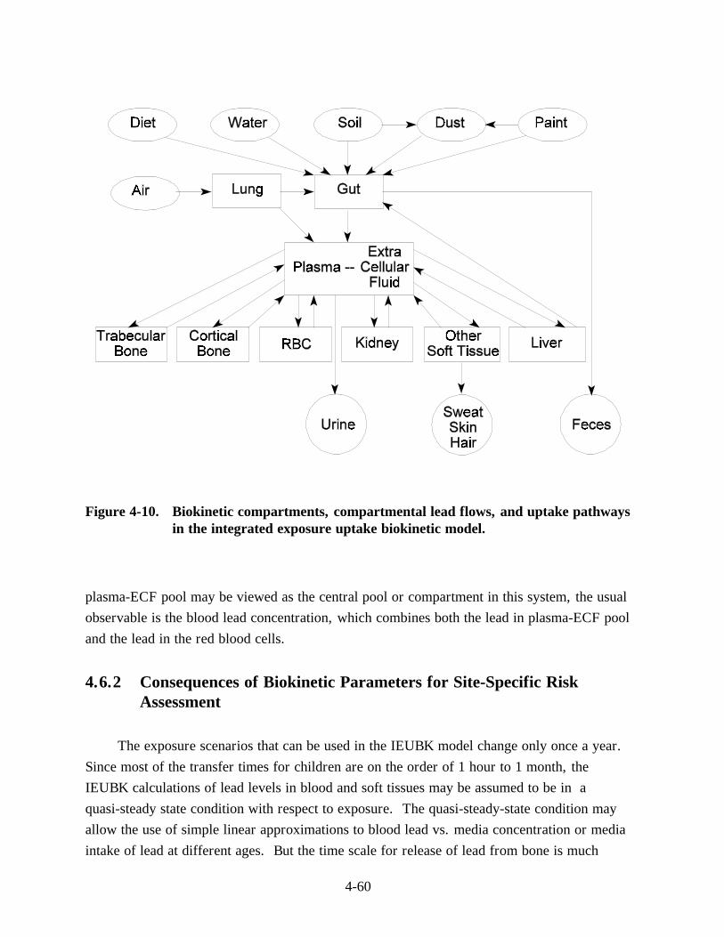
Figure 4-10. Biokinetic compartments, compartmental lead flows, and uptake pathways in the integrated exposure uptake biokinetic model.

plasma-ECF pool may be viewed as the central pool or compartment in this system, the usual observable is the blood lead concentration, which combines both the lead in plasma-ECF pool and the lead in the red blood cells.

4.6.2 Consequences of Biokinetic Parameters for Site-Specific Risk Assessment

The exposure scenarios that can be used in the IEUBK model change only once a year. Since most of the transfer times for children are on the order of 1 hour to 1 month, the IEUBK calculations of lead levels in blood and soft tissues may be assumed to be in a quasi-steady state condition with respect to exposure. The quasi-steady-state condition may allow the use of simple linear approximations to blood lead vs. media concentration or media intake of lead at different ages. But the time scale for release of lead from bone is much

4-60

longer, on the order of 1 to 3 years, so that the bone lead level quickly builds up and the skeleton contains 60 to 70 percent of the total body burden of lead by age 2 years. There is not be a true steady-state blood lead level during the 7-year interval used in the IEUBK model for young children. As bone lead burdens increase, so will there be a growing component of lead in blood that comes from release of lead from the skeleton or from resorption of bone in growing children.

Because of this release of bone lead, there may be a large component of blood lead levels in children that will respond only slowly to any changes in environmental lead exposure. This is particularly noticeable in evaluating soil lead abatement studies and strategies, where a child may have accumulated a large body burden of lead before the abatement. In the first year or two after the abatement, the internal or endogenous source oflead stored in the skeleton may cause a moderately elevated blood lead level to persist in the child. Children who were never exposed to the elevated environmental lead, or who did not accumulate a large body burden of lead before the abatement even though the environmental exposure was high, will not have this residual elevation of blood lead from resorbed bone lead.

4.7 ISSUES IN USE OF THE MODEL FOR PAINT CHIPS

4.7.1 Inappropriateness of Use of IEUBK Model for Paint Chip Ingestion

The IEUBK model, Version 1.0, does not contain an explicit component for lead-based paint ingestion outside of the Alternate Source Option in the Soil/Dust Menu. The correct use of the IEUBK model is to estimate geometric mean blood lead levels and distributions of blood lead levels in young children who have long-term chronic exposures to lead. It has long been known that the ingestion of even tiny quantities of paint chips on a single occasion can cause serious lead intoxication. Chisolm and Harrison (1956) show photographs of small paint chips weighing several grams that can easily be removed and eaten by a child. Since old lead-based paints can contain in excess of 50 percent lead, the child may ingest several million micrograms of lead in a single episode. The IEUBK model is not intended to address this situation. The IEUBK model is intended to address the situation where the child ingests typical quantities of household dust that have been contaminated by leaded soils and by deterioration of old lead-based paint from interior surfaces. The inclusion of lead-based paint in the dust menu implicitly assumes that paint has fallen off the painted surface as fine particles, or has fallen off as discrete flakes or chips of paint and has been reduced to small

4-61

particles in situ on the floor, carpet, furniture or other surfaces. Interior lead-based paint may not wear as rapidly as exterior paint due to the near-absence of sunlight on most household surfaces, but common observation finds many deteriorated lead-painted interior surfaces in older housing, especially in wet rooms such as kitchens, bathrooms, or laundry rooms (HUD, 1991).

The following data are presented to assist the user who wishes to develop an exposure scenario in which there is long-term ingestion of chips of lead-based paint, in addition to the interior household dust lead contribution that is already included in the IEUBK model. An exposure scenario with paint chip ingestion can be entered in the Other Source Menu of the model. The data for construction of an alternative lead-based paint chip menu were reviewed by the EPA Technical Review Work Group, who concluded that these data were not adequate to be recommended as default values. There are greater uncertainties about paint chip exposure and uptake than about other exposure media. These uncertainties include:

(1) The quantity of paint chips ingested on a long-term or chronic basis is unknown; however, even small quantities of ingested paint chips can produce a lead intake of millions of micrograms per day, overwhelming all other sources.

(2) Lead levels in housing are most typically measured as surface loadings using portable XRF analyzers. While there are several proposed relationships between lead paint surface loading and daily lead intake, these require making assumptions about other uncertain relationships, such as the "area" of surface ingested the child, or the thickness of the paint chip and the relationship between lead concentration and lead loading. We will describe these relationships, but we believe that they do not yet have an adequate empirical basis.

(3) Paint chips are, by definition, discrete units. Even if paints chips are at least one millimeter in diameter, or even larger, they may not be completely dissolved in the stomach or completely absorbed in the intestines. Observations of child fecal samples sometimes find discrete paint chips. Radio-opaque samples in stool may be lead or some mixture of lead with other heavy metals such as barium or chromium commonly found in leaded paint pigments.

4-62

(4) Lead paint absorption by rats has been found to depend significantly on particle size and chemical speciation of paint particles. Many chemical species are found in lead-based paint, most often including lead octoate (as a dryer), lead carbonate, and lead chromate. The sequence of absorption or bioavailability is probably

carbonate > octoate > chromate

based on rodent studies (Barltrop and Meek, 1979). While the ranking is probably similar in human children and other primates , direct evidence is limited to baboons (Cohen, 1975; Mallon, 1983). Studies are currently in progress using miniature swine as closely analogous models of human gastro-intestinal absorption of nutrients and contaminants, but results on absorption of lead from actual lead paints have not yet been reported. It is clear in any case that estimates of lead bioavailability in paints may require a much more complete site-specific characterization by particle size and chemical speciation than does soil.

4.7.2 Daily Intake of Paint Chips

The American Academy of Pediatrics (1972) has used a provisional estimate of one square inch (6.25 cm2) of paint surface ingested per day. This appears to be a nominal value for purposes of risk estimation, and no empirical basis for this value has been provided. They cite evidence that 1 cm2 of one layer of interior paint may weigh 5.0 to 8.2 mg (average 6.5 mg), and that six layers of paint weighed 37.0 to 40.6 mg (average 38.8). Thus, using data that may represent Providence RI in 1972, where six layers of paint were typical, ingestion of 6.25 cm2 of painted surface through a single painted layer would correspond to 40.6 mg/day intake, and a thick chip containing six layers would average 233 mg/d paint chip intake. Even if the ingested paint chips were square-inch monolayers with one percent lead, the daily lead intake would be 400 ug Pb/d. We cannot provide any realistic estimate of the uncertainty of this estimate. It is likely that there is some correlation between the size, thickness, and lead content of ingested paint chips, since additional lead is reported to add a sweet taste to the chips that may appeal to a child with pica for lead paint chips.

These estimates were also cited in a report by the National Academy of Sciences (NAS, 1973) to the Consumer Product Safety Commission (CPSC). They concluded that the quantitative evidence was inadequate "to promulgate a standard based on knowledge of the

4-63

essential quantitative relations that link the lead content of paint to symptoms of intoxication. However, this is not unusual in public-health practice. Many useful standards have been established by informed people who make judgments based on whatever facts are available" (NAS, 1973, pp. 25-26).

In view of the lower quality of information on paint chip intake than on intake of soil and dust, diet, and drinking water, and the usefulness of providing baseline risk assessments in the absence of lead-based paint, we have used a default value of 0 Fg/dL in the model.

4.7.3 Relationship of XRF Lead Paint Surface Loading to Lead Paint Concentration

The estimate of lead intake from paint chip ingestion depends on a lead concentration for the ingested chips. However, this is not available in field samples without removing a piece of paint from the wall or trim. Therefore, the use of non-destructive field sampling methods such as portable XRF analyzers has become the common method for determining paint hazard. We can calculate

lead concentration (Fg/g) = 0.001 (Fg/mg) * lead loading (mg/cm2) /

thickness of paint (cm) * paint density (g/cm3).

Calculations from the EPA Lead Reference Materials Workshop (EPA 1991) assuming a seven-layer thickness of paint (40 mil = 1 mm) and a density of 2 g/cm3 calculates 5,000 Fg/g equivalent to 1 mg/cm2. This is reasonably concordant with some analyses of measurements of paint loading and concentration that we had calculated from data in the Boston Brigham and Women's Hospital Longitudinal Lead Study. However, this relationship is likely to vary so greatly from house to house that we cannot recommend its use without site-specific verification.

4.7.4 Dissolution of Paint Chips in Acid Environments

Not all of the lead in a large lead paint chip may be available for absorption. Roberts et al. (1974) report that "20 to 60 percent of the lead in surface soil was extractable in 0.1N HCl compared with less than 10 percent extractable from paint samples." Particle dissolution is a component of lead bioavailability.

4-64

4.7.5 Absorption of Lead Paint In Vivo

The absorption of lead-based paint particles by rats is described in (Barltrop and Meek 1979). They conclude that "The physical form of particles derived from paint film would seem to modify the availability of Pb compounds contained in them for absorption. Little is known of the physical or chemical changes which paint flakes undergo after ingestion, although it is known that some paint flakes remain relatively intact when swallowed by a child and may be observed radiographically in the gut lumen, or on inspection of feces. In spite of this, sufficient absorption of Pb resulting in childhood poisoning is known to occur, and in many cases the ingested flakes become too finely divided to be visible macroscopically. Thus the composition of the paint and the chemical nature of the added Pb compounds may determine its stability in the gut and hence the availability of Pb for absorption. Long-term feeding of paint flakes identical to those used in this work, but of larger size (500 to 1,000 microns) have been reported to result in minimal absorption by the rat (Barltrop and Meek, 1975)."

Table 4-4 summarizes their results. Lead absorption can be characterized by the difference in blood lead levels between exposed and control rats. The increase in blood lead for rats fed lead octoate in particles between 500 and 1,000 microns diameter is about 60 percent of the absorption of lead octoate particles <50 microns, and absorption of lead chromate paint in particles of 500 to 1,000 microns is about 45 percent of the absorption of lead chromate paint in particles of 500 to 1,000 microns. For particles <50 microns, the increase in blood lead for lead octoate particles is about 60 percent of the increase from lead acetate. It is not clear how these results can be used quantitatively for humans to determine absolute or relative bioavailability of LBP.

Juvenile and infant baboons were exposed to oral intakes of lead salts and prepared lead paint samples from New York City (Mallon, 1983). The lead salts and paint samples were fed in gelatin capsules to sedated baboons. The relative bioavailability could be estimated from differences in the steady-state blood lead levels achieved after 5 or 6 months of chronic exposure. These are shown in Tables 4-5 and 4-6. The increase in blood lead in infant baboons (age 6 months at the start of the study) was 23 Fg/dL (no s.e.) for 2 baboons exposed to lead acetate and 6.125 Fg/dL for 8 baboons exposed to New York city paint at a controlled dose of 100 Fg/kg/day (roughly 250 to 350 Fg/day in baboons who grew from 2.5 to 3.5 kg body weight). At higher doses, the increases in blood lead were clearly nonlinear with respect to dose rate. In juvenile baboons (ages 20-24 months at the beginning of the study) the increase in blood lead was 11.7 Fg/dL (no s.e.) for 2 baboons exposed to

4-65

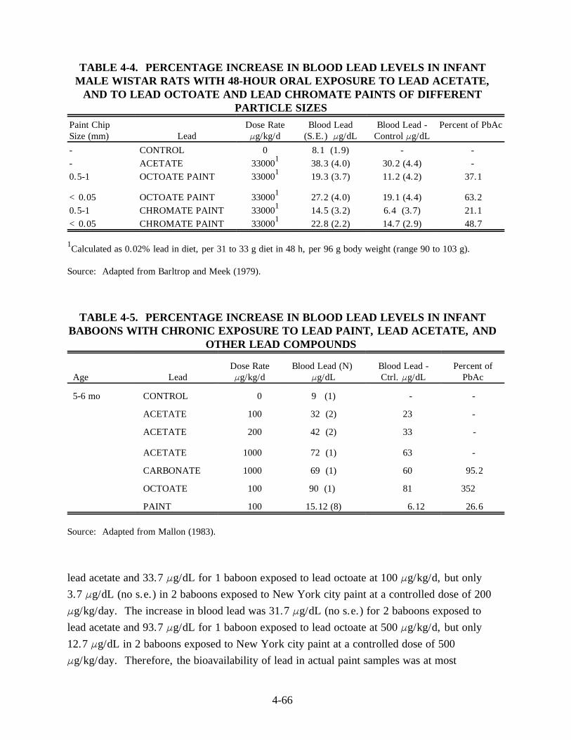
TABLE 4-4. PERCENTAGE INCREASE IN BLOOD LEAD LEVELS IN INFANT MALE WISTAR RATS WITH 48-HOUR ORAL EXPOSURE TO LEAD ACETATE,

AND TO LEAD OCTOATE AND LEAD CHROMATE PAINTS OF DIFFERENT PARTICLE SIZES

Paint Chip Dose Rate Blood Lead Blood Lead - Percent of PbAc Size (mm) Lead Fg/kg/d (S.E.) Fg/dL Control Fg/dL

- CONTROL 0 8.1 (1.9) - -- ACETATE 330001 38.3 (4.0) 30.2 (4.4) -0.5-1 OCTOATE PAINT 330001 19.3 (3.7) 11.2 (4.2) 37.1

<0.05 OCTOATE PAINT 330001 27.2 (4.0) 19.1 (4.4) 63.2 0.5-1 CHROMATE PAINT 330001 14.5 (3.2) 6.4 (3.7) 21.1 <0.05 CHROMATE PAINT 330001 22.8 (2.2) 14.7 (2.9) 48.7

1Calculated as 0.02% lead in diet, per 31 to 33 g diet in 48 h, per 96 g body weight (range 90 to 103 g).

Source: Adapted from Barltrop and Meek (1979).

TABLE 4-5. PERCENTAGE INCREASE IN BLOOD LEAD LEVELS IN INFANT BABOONS WITH CHRONIC EXPOSURE TO LEAD PAINT, LEAD ACETATE, AND

OTHER LEAD COMPOUNDS

Dose Rate Blood Lead (N) Blood Lead - Percent of Age Lead Fg/kg/d Fg/dL Ctrl. Fg/dL PbAc

5-6 mo CONTROL

ACETATE

ACETATE

ACETATE

CARBONATE

OCTOATE

PAINT

0 9 (1) - -

100 32 (2) 23 -

200 42 (2) 33 -

1000 72 (1) 63 -

1000 69 (1) 60 95.2

100 90 (1) 81 352

100 15.12 (8) 6.12 26.6

Source: Adapted from Mallon (1983).

lead acetate and 33.7 Fg/dL for 1 baboon exposed to lead octoate at 100 Fg/kg/d, but only 3.7 Fg/dL (no s.e.) in 2 baboons exposed to New York city paint at a controlled dose of 200 Fg/kg/day. The increase in blood lead was 31.7 Fg/dL (no s.e.) for 2 baboons exposed to lead acetate and 93.7 Fg/dL for 1 baboon exposed to lead octoate at 500 Fg/kg/d, but only 12.7 Fg/dL in 2 baboons exposed to New York city paint at a controlled dose of 500 Fg/kg/day. Therefore, the bioavailability of lead in actual paint samples was at most

4-66

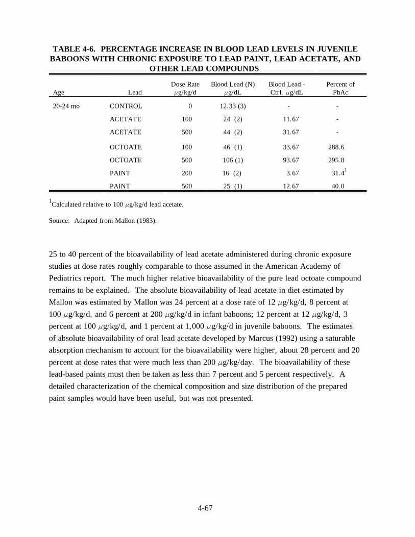
TABLE 4-6. PERCENTAGE INCREASE IN BLOOD LEAD LEVELS IN JUVENILEBABOONS WITH CHRONIC EXPOSURE TO LEAD PAINT, LEAD ACETATE, AND

OTHER LEAD COMPOUNDS

Dose Rate Blood Lead (N) Blood Lead - Percent of Age Lead Fg/kg/d Fg/dL Ctrl. Fg/dL PbAc

20-24 mo CONTROL 0 12.33 (3) - -

ACETATE 100 24 (2) 11.67 -

ACETATE 500 44 (2) 31.67 -

OCTOATE 100 46 (1) 33.67 288.6

OCTOATE 500 106 (1) 93.67 295.8

PAINT 200 16 (2) 3.67 31.41

PAINT 500 25 (1) 12.67 40.0

1Calculated relative to 100 Fg/kg/d lead acetate.

Source: Adapted from Mallon (1983).

25 to 40 percent of the bioavailability of lead acetate administered during chronic exposure studies at dose rates roughly comparable to those assumed in the American Academy of Pediatrics report. The much higher relative bioavailability of the pure lead octoate compound remains to be explained. The absolute bioavailability of lead acetate in diet estimated by Mallon was estimated by Mallon was 24 percent at a dose rate of 12 Fg/kg/d, 8 percent at 100 Fg/kg/d, and 6 percent at 200 Fg/kg/d in infant baboons; 12 percent at 12 Fg/kg/d, 3 percent at 100 Fg/kg/d, and 1 percent at 1,000 Fg/kg/d in juvenile baboons. The estimates of absolute bioavailability of oral lead acetate developed by Marcus (1992) using a saturable absorption mechanism to account for the bioavailability were higher, about 28 percent and 20 percent at dose rates that were much less than 200 Fg/kg/day. The bioavailability of these lead-based paints must then be taken as less than 7 percent and 5 percent respectively. A detailed characterization of the chemical composition and size distribution of the prepared paint samples would have been useful, but was not presented.

4-67