4. TECHNOLOGY DEVELOPMENT FOR ESTIMATING ......4-1 4. Technology Development for Estimating Forest Carbon Stocks 4.1. Outline of Technology Development for Gauging Forest Carbon Stocks

4. TECHNOLOGY DEVELOPMENT FOR ESTIMATING FOREST CARBON STOCKS

4-1

4. Technology Development for Estimating Forest Carbon Stocks

4.1. Outline of Technology Development for Gauging Forest Carbon Stocks

Technology development utilizing satellite remote sensing was carried out in order to estimate forest carbon stocks.

In the Study last year, gauging of the Tier 3 forest carbon stock in test sites (10 km x 10 km) and estimation of the wall-to-wall Tier 1 forest carbon stock using the FRA2000 Ecological Zone (FAO) was carried out in Louangphabang Province and Khamkeut District in Bolikhamxai Province.

This year, technology development was conducted with a view to enhancing the estimation accuracy of forest carbon stocks on the provincial and district levels. Figure 4-1 shows the flow chart for gauging forest carbon stock. The main processes involved are as follows.

A) Forest survey (to compare and verify with the rough forest conditions and satellite images in target area)

B) Analysis of forest carbon stock and measured tree heights (based on the results of forest survey)

C) Analysis of measured tree heights and PRISM measured tree heights (validity of PRISM tree height measurements)

D) Analysis of satellite images and forest stand factors (potential for forest classification based on satellite images)

E) Biomass classing based on satellite images

F) Analysis of the relationship between biomass class and tree height

G) Preparation of forest carbon stock estimation maps based on biomass classing

Carbon Stock Estimation FlowALOSPRISM

Field

Tree Height

CarbonStock

LivingBiomass

LANDSAT

TM

DBH

ALOSAVNIR2

CorrelationAnalysis

Correlation

Tree Height(Study point)

VerificationTree Height(Mesh grid)

Verification

3 Typeclassification(Current F.)

Accuracy

Visual Interpretation

(Grid)

CS‐TreeHeightModel

Mean Treeheight

Relation analysis

Figure 4-1 Flow Chart of Forest Carbon Stock Estimation

4-2

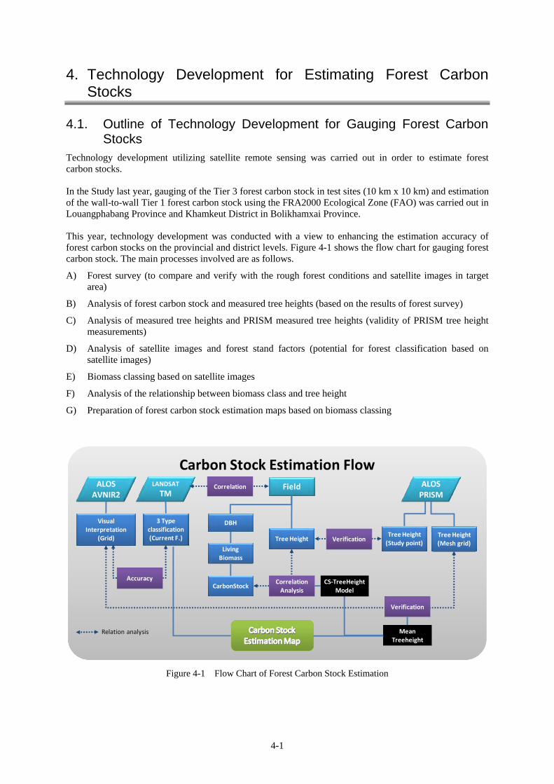
Tier levels have been defined according to the IPCC tier requirements stated in the GOFC-GOLD SOURCE BOOK (COP16 Version1 P2-46, Table 4-1).

According to this, data availability is an important item to consider when selecting the appropriate tier. In Tier 1, whereas the data requirement is low, in Tier 3, data are required on the level of national forest resources survey.

Moreover, the data used for gauging forest carbon stock in each tier are configured as follows (see Table 4-1).

Table 4-1 Data Requirements in Each IPCC Tier

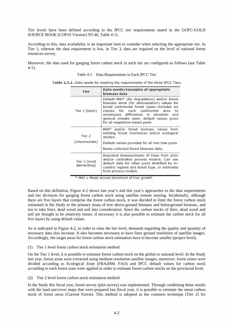
Based on this definition, Figure 4-2 shows last year’s and this year’s approaches to the data requirements and tier divisions for gauging forest carbon stock using satellite remote sensing. Incidentally, although there are five layers that comprise the forest carbon stock, it was decided to limit the forest carbon stock estimated in the Study to the primary strata of tree above-ground biomass and belowground biomass, and not to take litter, dead wood and soil into consideration. Since the carbon stocks of litter, dead wood and soil are thought to be relatively minor, if necessary it is also possible to estimate the carbon stock for all five layers by using default values.

As is indicated in Figure 4-2, in order to raise the tier level, demands regarding the quality and quantity of necessary data also increase. It also becomes necessary to have finer ground resolution of satellite images. Accordingly, the target areas for forest carbon stock estimation have to become smaller (project level).

(1) Tier 1 level forest carbon stock estimation method

On the Tier 1 level, it is possible to estimate forest carbon stock on the global or national level. In the Study last year, forest areas were extracted using medium resolution satellite images; moreover, forest zones were divided according to Ecological Zone (FRA2000, FAO) and IPCC default values for carbon stock according to each forest zone were applied in order to estimate forest carbon stocks on the provincial level.


In the Study this fiscal year, forest survey (plot survey) was implemented. Through combining these results with the land use/cover maps that were prepared last fiscal year, it is possible to estimate the mean carbon stock of forest areas (Current Forest). This method is adopted as the common technique (Tier 2) for

4-3

estimating forest carbon stock through combining satellite remote sensing and ground survey. However, this technique does require a lot of plot surveys.

The forest carbon stock estimation model that adopts tree crown density as a parameter can also be considered, however, a standard approach for accurately estimating tree crown density (for example, less than 20 percent, 20~40 percent, 40~70 percent, and 70~100 percent) from medium resolution satellite images on the national or sub-national level is still in the research stage and has not yet been developed for practical application.

As a result of implementing forest survey in the Study, crown density at all the plot survey points was 70 percent or higher (dense forest stand) and the forest type was almost entirely broad-leaved evergreen forest. In the Study this year, using the Tier 2-1 findings as reference data, the mean forest carbon stock was estimated from land use/cover maps and forest survey results assuming tree crown density of 70 percent or higher and forest type of broad-leaved evergreen forest.

(3) Tier 2-2 level forest carbon stock estimation method (CS-H model)

In this fiscal year, as a Tier 2 forest carbon stock estimation method, forest survey (plot survey) was implemented and forest carbon stock was estimated based on forest biomass classes (three classes) utilizing satellite image spectral images, forest survey, the IPCC recommended forest carbon stock model and the forest carbon stock-tree height model that applies satellite image analysis (CS-H model).


In order to gauge the Tier 3 forest carbon stock, it is necessary to implement periodic national forest resources survey and adopt a model that corresponds to the area and forest types and tree species, etc. Accordingly, when it comes to gauging Tier 3 forest carbon stock on the national scale in developing countries, it takes a huge amount of time and effort.

However, this can be done on the project level, where the target area is limited, and research has been conducted on forest management and gauging of forest carbon stock based on a GIS forest register.

4-4

Tier2-2

Tier3

Tier1

Tier2-1

Low Satellite resolution High

Land use/cover maps IPCC existing values

Ecological Zone

Land use/covermaps Forest (plot) inventoryIPCC existing values

Ecological Zone Using FRA2000, FAO, divide the forest zones and estimate forest carbon stock from IPCC existing values.

Apply the mean carbon stock calculated from forest

inventory and IPCC existing values to forest areas in land use/cover maps, and estimate

the overall forest carbon stock

Forest type divisionForest section

maps, forest registers

Unique model

Define a unique model according to national forest resources survey and monitoring forest inventory, etc., and estimate carbon stock using the GIS base forest managementsystem.

Low

Dat

a re

qu

irem

ent

Hig

h

Low Tier level High

Legend

High

Medium

Low

Land use/covermaps Biomass classification

mapsForest (plot) inventoryIPCC existing values

CS-H model*

Define the model from the correlation of forest inventory with IPCC existing values and tree heights, divide forest into three classes according to biomass and estimate the forest carbon stock in each.

Ecological zone‐separate forest carbon stock

Land use/cover mapBiomass class‐separate forest carbon stock

Forest carbon stock estimation map based on

Figure 4-2 Relation between Tier Level, Satellite Image Resolution, Target Area and Data Requirements

4-5

4.2. Forest Survey 4.2.1. Objectives of Forest Survey

Forest survey was carried out with the aims of analyzing the relationship between forest carbon stock and tree height, analyzing the accuracy of tree height measurements based on ALOS/PRISM, analyzing the correlation between ALOS/AVNIR2 biomass classes and LANDSAT/TM satellite images, and so on. The following sections describe the methodology and results.

4.2.2. Forest Survey Methodology

The widely adopted standard forest survey method was used to conduct forest survey. Squares of 20 m x 20 m were adopted as the standard plots, while 10 m x 10 m was adopted in areas where the mean tree height was less than 10 m.

Survey candidate locations were selected in advance from the areas (Current Forest) covered by the land use/cover maps prepared last year. In making the selection, reference was made to the visual interpretation results using the ALOS/AVNIR2 images described in Chapter 2, Google Earth, topographical maps and existing road maps and consideration was given to the local accessibility, etc. The following paragraphs describe the survey items, used equipment and caution points in setting the survey plots.

(1) Access to survey plots

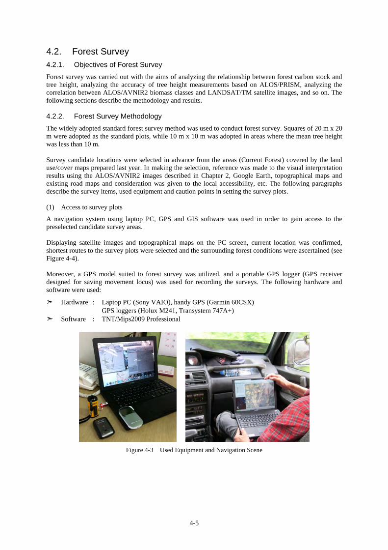
A navigation system using laptop PC, GPS and GIS software was used in order to gain access to the preselected candidate survey areas.

Displaying satellite images and topographical maps on the PC screen, current location was confirmed, shortest routes to the survey plots were selected and the surrounding forest conditions were ascertained (see Figure 4-4).

Moreover, a GPS model suited to forest survey was utilized, and a portable GPS logger (GPS receiver designed for saving movement locus) was used for recording the surveys. The following hardware and software were used:

➣ Hardware : Laptop PC (Sony VAIO), handy GPS (Garmin 60CSX) GPS loggers (Holux M241, Transystem 747A+)

➣ Software : TNT/Mips2009 Professional

Figure 4-3 Used Equipment and Navigation Scene

4-6

(2) Survey items

The forest survey items were as follows.

A) Upper tree height : The five or six highest trees out of those with greater diameter at breast height than the mean in the plot stand were selected, and tree height measurement was conducted in units of 10 cm using the ultrasonic measurement device Vertex.

B) Diameter at breast height (DBH) : A tape measure was used to measure in centimeters the DBH of all trees with a breast height diameter of 5 cm or more inside the plot. In cases were measurement with the tape measure was difficult, a 2 m red and white pole was used instead.

C) Major tree species : The major tree species inside the plot were determined. All the tree species inside the plot were identified, and all the determined species names were recorded. Local names were recorded in the field notebook and were later changed to scientific names.

D) State of lower level vegetation : Three classifications of Dense, Medium and Sparse were determined based on visual inspection.

E) Aspect : Eight orientations (N/NE/E/ES/S/SW/S/NS) were measured using compass and clinometer.

F) Slope : Slope in the aspect was measured in degrees using compass and clinometer.

G) Stand photographs : Photographs were taken of the forest stand, lower layer, crown and surface conditions.

H) Survey plot coordinates : Using the handy GPS, latitude and longitude coordinates were measured in the four corners of the survey plots.

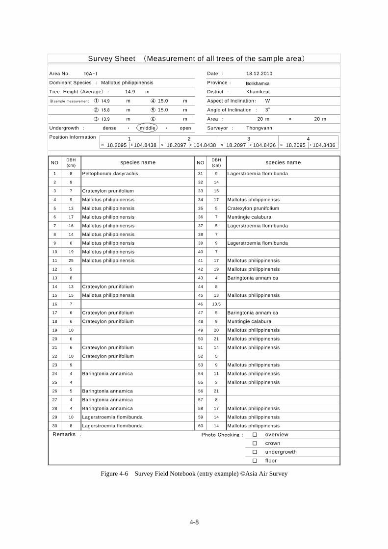
※ Figure 4-5 shows a scene from the forest survey, and Figure 4-6 shows an example of field notebook entry.

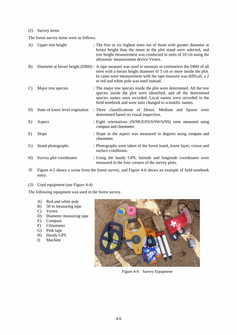
(3) Used equipment (see Figure 4-4)

The following equipment was used in the forest survey.

A) Red and white pole B) 50 m measuring tape C) Vertex D) Diameter measuring tape E) Compass F) Clinometer G) Pink tape H) Handy GPS I) Machete

Figure 4-4 Survey Equipment

4-7

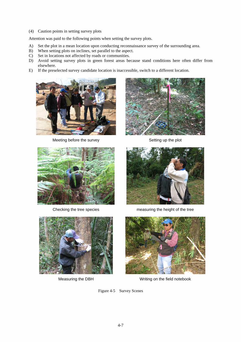
(4) Caution points in setting survey plots

Attention was paid to the following points when setting the survey plots.

A) Set the plot in a mean location upon conducting reconnaissance survey of the surrounding area. B) When setting plots on inclines, set parallel to the aspect. C) Set in locations not affected by roads or communities. D) Avoid setting survey plots in green forest areas because stand conditions here often differ from

elsewhere. E) If the preselected survey candidate location is inaccessible, switch to a different location.

Meeting before the survey Setting up the plot

Checking the tree species measuring the height of the tree

Measuring the DBH Writing on the field notebook

Figure 4-5 Survey Scenes

4-8

Area No． 10Ａ-1 Date　： 18.12.2010

Dominant Species　： Mallotus philippinensis Province ： Borikhamxai

Tree　Height （Average）　： 14.9 m District　： Khamkeut

14.9 m ④ 15.0 m Aspect of Inclination： W

② 15.8 m ⑤ 15.0 m Angle of Inclination　： 3°

③ 13.9 m ⑥ m Area　： 20 m × 20 m

Undergrowth　： dense ・ middle ・ open Surveyor　： Thongvanh

Position Information

NODBH(cm)

NODBH(cm)

1 8 Peltophorum dasyrachis 31 9 Lagerstroemia flomibunda

2 9 32 14

3 7 Cratexylon prunifolium 33 15

4 9 Mallotus philippinensis 34 17 Mallotus philippinensis

5 13 Mallotus philippinensis 35 5 Cratexylon prunifolium

6 17 Mallotus philippinensis 36 7 Muntingie calabura

7 16 Mallotus philippinensis 37 5 Lagerstroemia flomibunda

8 14 Mallotus philippinensis 38 7

9 6 Mallotus philippinensis 39 9 Lagerstroemia flomibunda

10 19 Mallotus philippinensis 40 7


12 5 42 19 Mallotus philippinensis

13 8 43 4 Baringtonia annamica



16 7 46 13.5

17 6 Cratexylon prunifolium 47 5 Baringtonia annamica

18 6 Cratexylon prunifolium 48 9 Muntingie calabura



21 6 Cratexylon prunifolium 51 14 Mallotus philippinensis



24 4 Baringtonia annamica 54 11 Mallotus philippinensis


26 5 Baringtonia annamica 56 21

27 4 Baringtonia annamica 57 8

28 4 Baringtonia annamica 58 17 Mallotus philippinensis

29 10 Lagerstroemia flomibunda 59 14 Mallotus philippinensis

30 8 Lagerstroemia flomibunda 60 14 Mallotus philippinensis

Photo Checking ： □ overview

□ crown

□ undergrowth

□ floor

species name species name

　Survey Sheet 　（Measurement of all trees of the sample area）

※sample measurement　　①

Remarks　：

18.2095 104.8438 18.2097 104.8438 18.2097 104.8436 18.2095 104.84361 2 3 4

N E N E N E N E

Figure 4-6 Survey Field Notebook (entry example) ©Asia Air Survey

Bolikhamxai

4-9

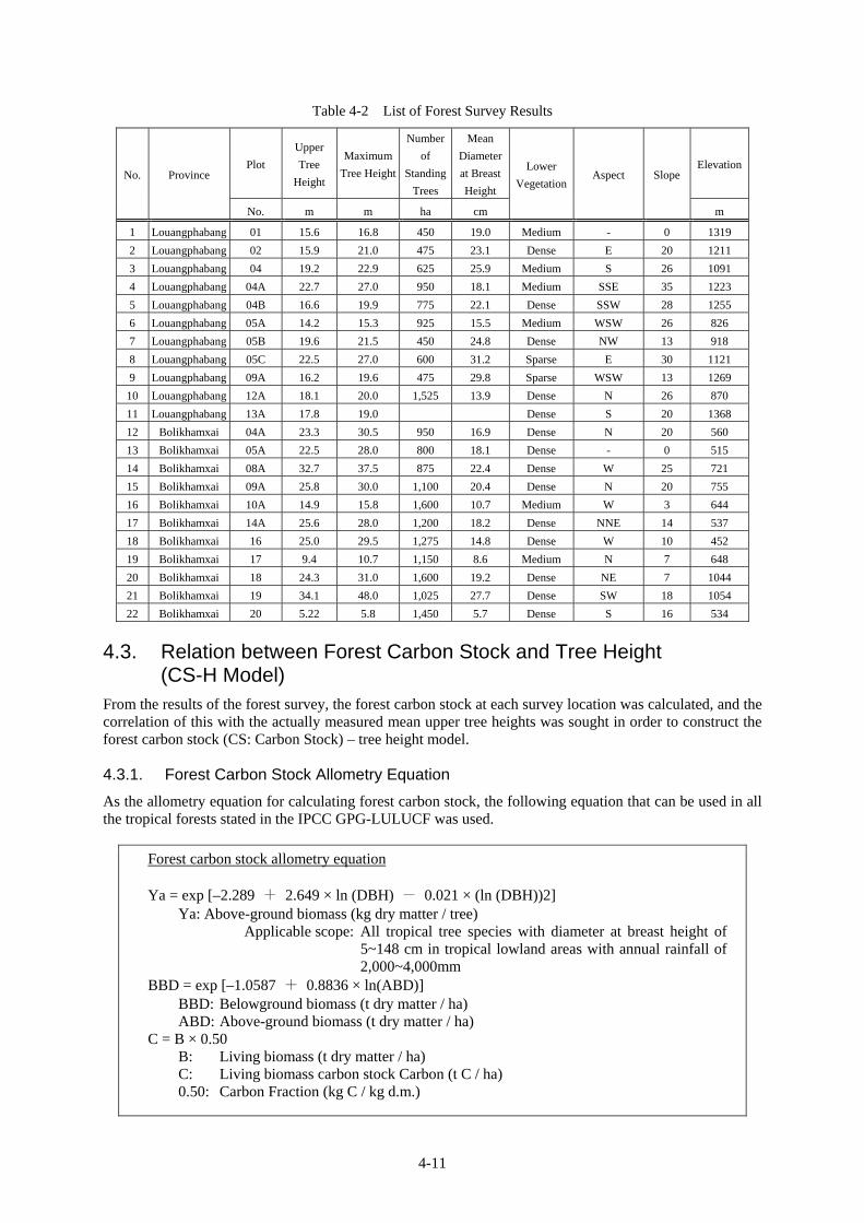
4.2.3. Forest Survey Results

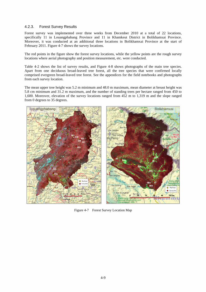
Forest survey was implemented over three weeks from December 2010 at a total of 22 locations, specifically 11 in Louangphabang Province and 11 in Khamkeut District in Bolikhamxai Province. Moreover, it was conducted at an additional three locations in Bolikhamxai Province at the start of February 2011. Figure 4-7 shows the survey locations.

The red points in the figure show the forest survey locations, while the yellow points are the rough survey locations where aerial photography and position measurement, etc. were conducted.

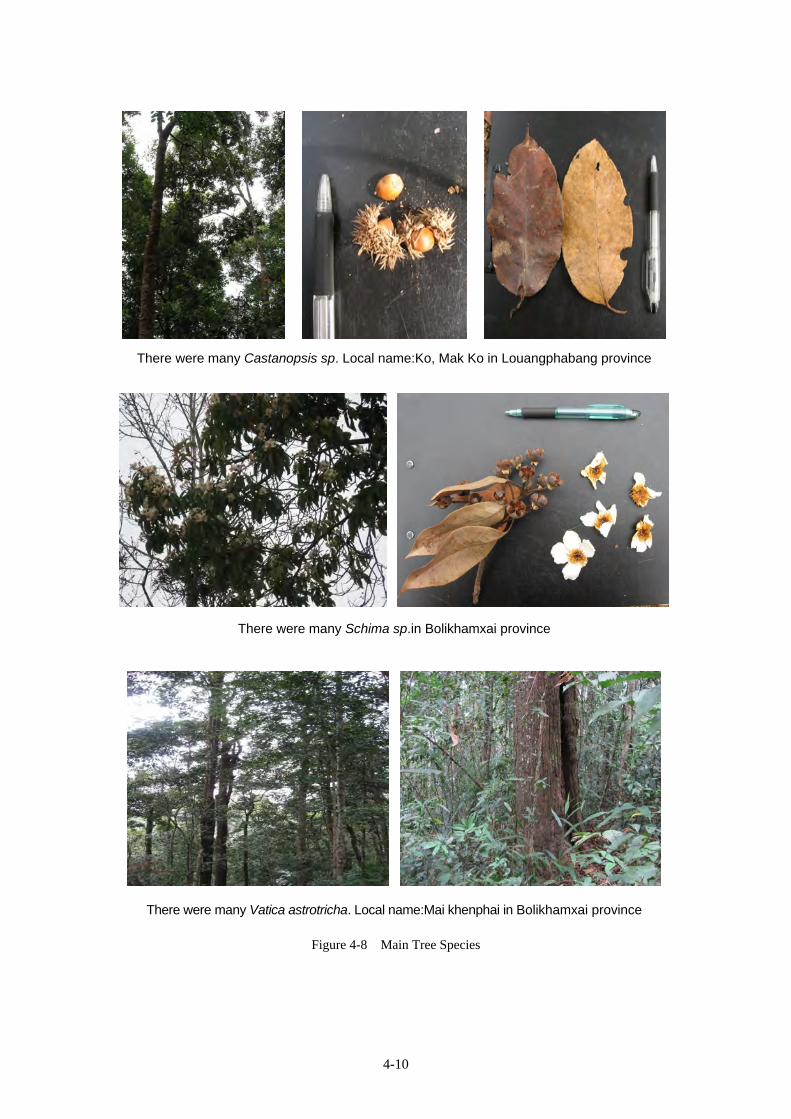
Table 4-2 shows the list of survey results, and Figure 4-8 shows photographs of the main tree species. Apart from one deciduous broad-leaved tree forest, all the tree species that were confirmed locally comprised evergreen broad-leaved tree forest. See the appendices for the field notebooks and photographs from each survey location.

The mean upper tree height was 5.2 m minimum and 48.0 m maximum, mean diameter at breast height was 5.8 cm minimum and 31.2 m maximum, and the number of standing trees per hectare ranged from 450 to 1,600. Moreover, elevation of the survey locations ranged from 452 m to 1,319 m and the slope ranged from 0 degrees to 35 degrees.

Figure 4-7 Forest Survey Location Map

Louangphabang Bolikhamxai

4-10

Figure 4-8 Main Tree Species

There were many Castanopsis sp. Local name:Ko, Mak Ko in Louangphabang province

There were many Schima sp.in Bolikhamxai province

There were many Vatica astrotricha. Local name:Mai khenphai in Bolikhamxai province

4-11

Table 4-2 List of Forest Survey Results

No. Province Plot

Upper

Tree

Height

Maximum

Tree Height

Number

of

Standing

Trees

Mean

Diameter

at Breast

Height

Lower

VegetationAspect Slope

Elevation

No. m m ha cm m

1 Louangphabang 01 15.6 16.8 450 19.0 Medium - 0 1319

2 Louangphabang 02 15.9 21.0 475 23.1 Dense E 20 1211

3 Louangphabang 04 19.2 22.9 625 25.9 Medium S 26 1091

4 Louangphabang 04A 22.7 27.0 950 18.1 Medium SSE 35 1223

5 Louangphabang 04B 16.6 19.9 775 22.1 Dense SSW 28 1255

6 Louangphabang 05A 14.2 15.3 925 15.5 Medium WSW 26 826

7 Louangphabang 05B 19.6 21.5 450 24.8 Dense NW 13 918

8 Louangphabang 05C 22.5 27.0 600 31.2 Sparse E 30 1121

9 Louangphabang 09A 16.2 19.6 475 29.8 Sparse WSW 13 1269

10 Louangphabang 12A 18.1 20.0 1,525 13.9 Dense N 26 870

11 Louangphabang 13A 17.8 19.0 Dense S 20 1368

12 Bolikhamxai 04A 23.3 30.5 950 16.9 Dense N 20 560

13 Bolikhamxai 05A 22.5 28.0 800 18.1 Dense - 0 515

14 Bolikhamxai 08A 32.7 37.5 875 22.4 Dense W 25 721

15 Bolikhamxai 09A 25.8 30.0 1,100 20.4 Dense N 20 755

16 Bolikhamxai 10A 14.9 15.8 1,600 10.7 Medium W 3 644

17 Bolikhamxai 14A 25.6 28.0 1,200 18.2 Dense NNE 14 537

18 Bolikhamxai 16 25.0 29.5 1,275 14.8 Dense W 10 452

19 Bolikhamxai 17 9.4 10.7 1,150 8.6 Medium N 7 648

20 Bolikhamxai 18 24.3 31.0 1,600 19.2 Dense NE 7 1044

21 Bolikhamxai 19 34.1 48.0 1,025 27.7 Dense SW 18 1054

22 Bolikhamxai 20 5.22 5.8 1,450 5.7 Dense S 16 534

4.3. Relation between Forest Carbon Stock and Tree Height (CS-H Model)

From the results of the forest survey, the forest carbon stock at each survey location was calculated, and the correlation of this with the actually measured mean upper tree heights was sought in order to construct the forest carbon stock (CS: Carbon Stock) – tree height model.

4.3.1. Forest Carbon Stock Allometry Equation

As the allometry equation for calculating forest carbon stock, the following equation that can be used in all the tropical forests stated in the IPCC GPG-LULUCF was used.

Forest carbon stock allometry equation Ya = exp [–2.289 ＋ 2.649 × ln (DBH) － 0.021 × (ln (DBH))2]

Ya: Above-ground biomass (kg dry matter / tree) Applicable scope: All tropical tree species with diameter at breast height of

5~148 cm in tropical lowland areas with annual rainfall of 2,000~4,000mm

BBD = exp [–1.0587 ＋ 0.8836 × ln(ABD)] BBD: Belowground biomass (t dry matter / ha) ABD: Above-ground biomass (t dry matter / ha)

C = B × 0.50 B: Living biomass (t dry matter / ha) C: Living biomass carbon stock Carbon (t C / ha) 0.50: Carbon Fraction (kg C / kg d.m.)

4-12

This equation is applicable to all tropical tree species having diameter at breast height of 5~148 cm in tropical lowland areas with annual rainfall of 2,000~4,000 mm. From the diameter at breast height, first the above-ground biomass and then the belowground biomass are calculated, and the combined total gives the living biomass stock. This is then multiplied by the carbon fraction in order to give the forest carbon stock.

Table 4-3 shows the calculated forest carbon stock and upper tree height s at each survey location.

Moreover, in cases where trees with diameter of less than 4 cm were confirmed in the local plot surveys, they were excluded from the calculation by this allometry equation.

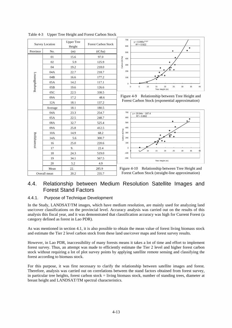
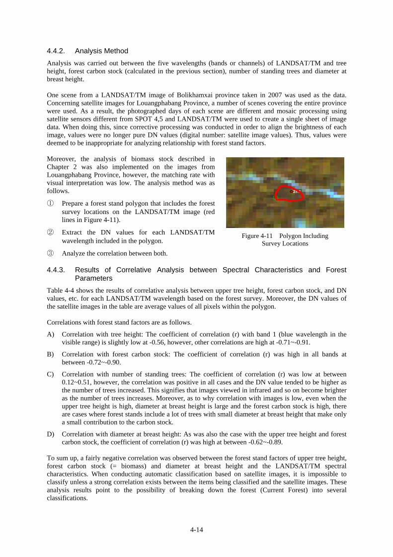
4.3.2. Forest Carbon Stock－Tree Height Model

Figure 4-9 and Figure 4-10 show the correlation between upper tree height s and forest carbon stock (Table 4-3). Since the correlation R2 based on exponential approximation is high at 0.9227, while the correlation R2 based on straight-line approximation is also high at 0.802, both figures indicate a high degree of correlation.

However, there were some cases where the forest carbon stock fluctuated even though the upper tree height was roughly the same. This is thought to be due to the fact that the relation between diameter at breast height and growth density is not uniform. For example, In survey plot Nos. 16 and 18 in Bolikhamxai Province, upper tree height was roughly the same at 25.0 m and 24.3 m respectively, however, the forest carbon stock showed a disparity of approximately 300 tC/ha between the 220.6 tC/ha in plot No. 16 and 519.0 tC/ha in No. 18. In plot No. 16, whereas the mean diameter at breast height was 14.8 cm and number of standing trees per hectare was 1,275, in plot No. 18 these figures were 19.2 cm and 1,600 trees respectively. Accordingly, the disparity in forest carbon stock arose from the differences in diameter at breast height and tree density.

However, since fluctuations were small and high correlation factors were observed in all the other plots, it was decided to adopt this approximation formula as the model (relational expression) for forest carbon stock and tree height.

Having said that, in the case of the straight-line approximation formula, since the forest carbon stock becomes negative at tree heights of less than 9 m, the following exponential approximation curve formula shown in Figure 4-9 was adopted as the forest carbon stock (CS) and tree height model.

Forest carbon stock (CS) - Tree height model C = 0.0959TH2.5373

C: Living biomass carbon stock, Carbon (t C / ha) TH: Upper tree height

4-13

Table 4-3 Upper Tree Height and Forest Carbon Stock

Survey Location Upper Tree

Height Forest Carbon Stock

Province No. (m) (tC/ha)

Louangphabang

01 15.6 97.0

02 5.9 125.9

04 19.2 218.0

04A 22.7 218.7

04B 16.6 177.2

05A 14.2 117.1

05B 19.6 126.6

05C 22.5 338.5

09A 17.2 48.6

12A 18.1 137.2

Average 18.1 180.5

Bolikham

xai

04A 23.3 254.7

05A 22.5 248.7

08A 32.7 525.4

09A 25.8 412.5

10A 14.9 68.2

14A 5.6 300.7

16 25.0 220.6

17 9. 22.4

18 24.3 519.0

19 34.1 567.5

20 5.2 4.9

Mean 22. 285.9

Overall mean 20.2 235.7

y = 0.095x2.537

R² = 0.922

0

100

200

300

400

500

600

700

0 5 10 15 20 25 30 35 40

Car

bo

n (ｔ

C/h

a)

Tree Height (m)

Figure 4-9 Relationship between Tree Height and Forest Carbon Stock (exponential approximation)

y = 20.94x - 187.4R² = 0.802

-200

-100

0

100

200

300

400

500

600

700

0 5 10 15 20 25 30 35 40

Car

bo

n (ｔ

C/h

a)

Tree Height (m)

Figure 4-10 Relationship between Tree Height and Forest Carbon Stock (straight-line approximation)

4.4. Relationship between Medium Resolution Satellite Images and Forest Stand Factors

4.4.1. Purpose of Technique Development

In the Study, LANDSAT/TM images, which have medium resolution, are mainly used for analyzing land use/cover classifications on the provincial level. Accuracy analysis was carried out on the results of this analysis this fiscal year, and it was demonstrated that classification accuracy was high for Current Forest (a category defined as forest in Lao PDR).

As was mentioned in section 4.1, it is also possible to obtain the mean value of forest living biomass stock and estimate the Tier 2 level carbon stock from these land use/cover maps and forest survey results.

However, in Lao PDR, inaccessibility of many forests means it takes a lot of time and effort to implement forest survey. Thus, an attempt was made to efficiently estimate the Tier 2 level and higher forest carbon stock without requiring a lot of plot survey points by applying satellite remote sensing and classifying the forest according to biomass stock.

For this purpose, it was first necessary to clarify the relationship between satellite images and forest. Therefore, analysis was carried out on correlations between the stand factors obtained from forest survey, in particular tree heights, forest carbon stock = living biomass stock, number of standing trees, diameter at breast height and LANDSAT/TM spectral characteristics.

4-14

4.4.2. Analysis Method

Analysis was carried out between the five wavelengths (bands or channels) of LANDSAT/TM and tree height, forest carbon stock (calculated in the previous section), number of standing trees and diameter at breast height.

One scene from a LANDSAT/TM image of Bolikhamxai province taken in 2007 was used as the data. Concerning satellite images for Louangphabang Province, a number of scenes covering the entire province were used. As a result, the photographed days of each scene are different and mosaic processing using satellite sensors different from SPOT 4,5 and LANDSAT/TM were used to create a single sheet of image data. When doing this, since corrective processing was conducted in order to align the brightness of each image, values were no longer pure DN values (digital number: satellite image values). Thus, values were deemed to be inappropriate for analyzing relationship with forest stand factors.

Moreover, the analysis of biomass stock described in Chapter 2 was also implemented on the images from Louangphabang Province, however, the matching rate with visual interpretation was low. The analysis method was as follows.

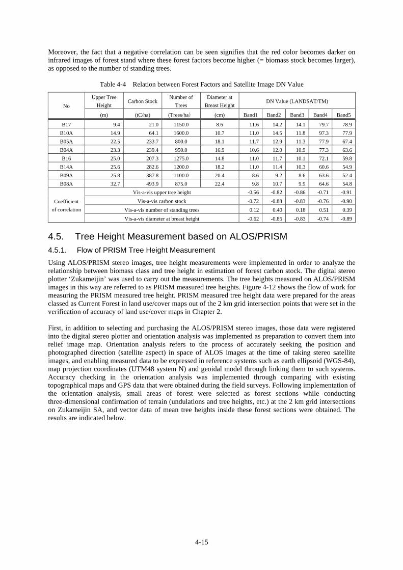
① Prepare a forest stand polygon that includes the forest survey locations on the LANDSAT/TM image (red lines in Figure 4-11).

② Extract the DN values for each LANDSAT/TM wavelength included in the polygon.

③ Analyze the correlation between both.

4.4.3. Results of Correlative Analysis between Spectral Characteristics and Forest Parameters

Table 4-4 shows the results of correlative analysis between upper tree height, forest carbon stock, and DN values, etc. for each LANDSAT/TM wavelength based on the forest survey. Moreover, the DN values of the satellite images in the table are average values of all pixels within the polygon.

Correlations with forest stand factors are as follows.

A) Correlation with tree height: The coefficient of correlation (r) with band 1 (blue wavelength in the visible range) is slightly low at -0.56, however, other correlations are high at -0.71~-0.91.

B) Correlation with forest carbon stock: The coefficient of correlation (r) was high in all bands at between -0.72~-0.90.

C) Correlation with number of standing trees: The coefficient of correlation (r) was low at between 0.12~0.51, however, the correlation was positive in all cases and the DN value tended to be higher as the number of trees increased. This signifies that images viewed in infrared and so on become brighter as the number of trees increases. Moreover, as to why correlation with images is low, even when the upper tree height is high, diameter at breast height is large and the forest carbon stock is high, there are cases where forest stands include a lot of trees with small diameter at breast height that make only a small contribution to the carbon stock.

D) Correlation with diameter at breast height: As was also the case with the upper tree height and forest carbon stock, the coefficient of correlation (r) was high at between -0.62~-0.89.

To sum up, a fairly negative correlation was observed between the forest stand factors of upper tree height, forest carbon stock (= biomass) and diameter at breast height and the LANDSAT/TM spectral characteristics. When conducting automatic classification based on satellite images, it is impossible to classify unless a strong correlation exists between the items being classified and the satellite images. These analysis results point to the possibility of breaking down the forest (Current Forest) into several classifications.

Figure 4-11 Polygon Including Survey Locations

4-15

Moreover, the fact that a negative correlation can be seen signifies that the red color becomes darker on infrared images of forest stand where these forest factors become higher (= biomass stock becomes larger), as opposed to the number of standing trees.

Table 4-4 Relation between Forest Factors and Satellite Image DN Value

No

Upper Tree

Height Carbon Stock

Number of

Trees

Diameter at

Breast HeightDN Value (LANDSAT/TM)

(m) (tC/ha) (Trees/ha） (cm) Band1 Band2 Band3 Band4 Band5

B17 9.4 21.0 1150.0 8.6 11.6 14.2 14.1 79.7 78.9

B10A 14.9 64.1 1600.0 10.7 11.0 14.5 11.8 97.3 77.9

B05A 22.5 233.7 800.0 18.1 11.7 12.9 11.3 77.9 67.4

B04A 23.3 239.4 950.0 16.9 10.6 12.0 10.9 77.3 63.6

B16 25.0 207.3 1275.0 14.8 11.0 11.7 10.1 72.1 59.8

B14A 25.6 282.6 1200.0 18.2 11.0 11.4 10.3 60.6 54.9

B09A 25.8 387.8 1100.0 20.4 8.6 9.2 8.6 63.6 52.4

B08A 32.7 493.9 875.0 22.4 9.8 10.7 9.9 64.6 54.8

Coefficient

of correlation

Vis-a-vis upper tree height -0.56 -0.82 -0.86 -0.71 -0.91

Vis-a-vis carbon stock -0.72 -0.88 -0.83 -0.76 -0.90

Vis-a-vis number of standing trees 0.12 0.40 0.18 0.51 0.39

Vis-a-vis diameter at breast height -0.62 -0.85 -0.83 -0.74 -0.89

4.5. Tree Height Measurement based on ALOS/PRISM 4.5.1. Flow of PRISM Tree Height Measurement

Using ALOS/PRISM stereo images, tree height measurements were implemented in order to analyze the relationship between biomass class and tree height in estimation of forest carbon stock. The digital stereo plotter ‘Zukameijin’ was used to carry out the measurements. The tree heights measured on ALOS/PRISM images in this way are referred to as PRISM measured tree heights. Figure 4-12 shows the flow of work for measuring the PRISM measured tree height. PRISM measured tree height data were prepared for the areas classed as Current Forest in land use/cover maps out of the 2 km grid intersection points that were set in the verification of accuracy of land use/cover maps in Chapter 2.

First, in addition to selecting and purchasing the ALOS/PRISM stereo images, those data were registered into the digital stereo plotter and orientation analysis was implemented as preparation to convert them into relief image map. Orientation analysis refers to the process of accurately seeking the position and photographed direction (satellite aspect) in space of ALOS images at the time of taking stereo satellite images, and enabling measured data to be expressed in reference systems such as earth ellipsoid (WGS-84), map projection coordinates (UTM48 system N) and geoidal model through linking them to such systems. Accuracy checking in the orientation analysis was implemented through comparing with existing topographical maps and GPS data that were obtained during the field surveys. Following implementation of the orientation analysis, small areas of forest were selected as forest sections while conducting three-dimensional confirmation of terrain (undulations and tree heights, etc.) at the 2 km grid intersections on Zukameijin SA, and vector data of mean tree heights inside these forest sections were obtained. The results are indicated below.

4-16

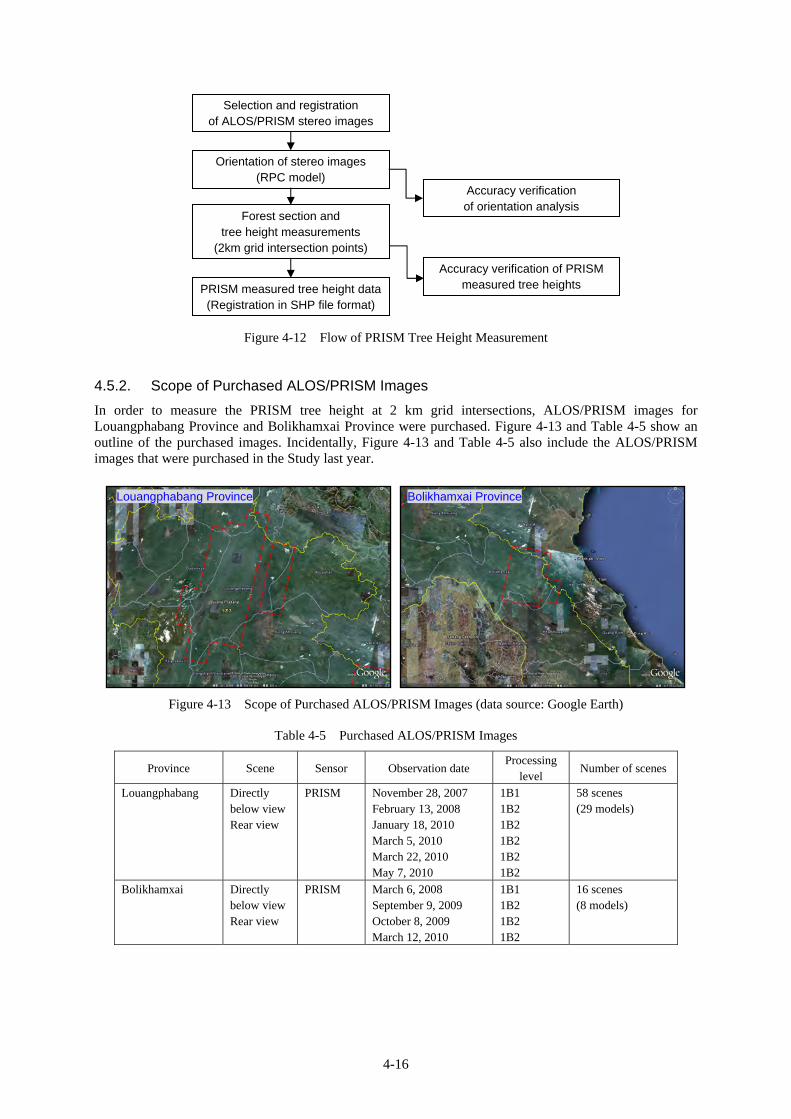
Figure 4-12 Flow of PRISM Tree Height Measurement 4.5.2. Scope of Purchased ALOS/PRISM Images

In order to measure the PRISM tree height at 2 km grid intersections, ALOS/PRISM images for Louangphabang Province and Bolikhamxai Province were purchased. Figure 4-13 and Table 4-5 show an outline of the purchased images. Incidentally, Figure 4-13 and Table 4-5 also include the ALOS/PRISM images that were purchased in the Study last year.

Figure 4-13 Scope of Purchased ALOS/PRISM Images (data source: Google Earth)

Table 4-5 Purchased ALOS/PRISM Images

Province Scene Sensor Observation date Processing

level Number of scenes

Louangphabang Directly below view Rear view

PRISM November 28, 2007 February 13, 2008 January 18, 2010 March 5, 2010 March 22, 2010 May 7, 2010

1B1 1B2 1B2 1B2 1B2 1B2

58 scenes (29 models)

Bolikhamxai Directly below view Rear view

PRISM March 6, 2008 September 9, 2009 October 8, 2009 March 12, 2010

1B1 1B2 1B2 1B2

16 scenes (8 models)

Selection and registration of ALOS/PRISM stereo images

Orientation of stereo images (RPC model)

Accuracy verification of orientation analysis

Forest section and tree height measurements

(2km grid intersection points)

PRISM measured tree height data(Registration in SHP file format)

Accuracy verification of PRISM measured tree heights

Louangphabang Province Bolikhamxai Province

4-17

4.5.3. Block Division of ALOS/PRISM Images for Three-dimensional Measurement

As preparation for implementing the tree height measurement, the purchased ALOS/PRISM images were divided into district blocks. Table 4-6 and Table 4-7 show the specifications of the image data in each block, while Figure 4-14 and Figure 4-15 show the ALOS/PRISM images. EGM96 was used to calculate the geoidal height.

Table 4-6 Specifications of Block Division in Louangphabang

Block Observed date Processing

level Scene ID

Number of scenes

LP① November 28, 2007 1B1 Directly below view : ALPSMN098183190~210

Rear view : ALPSMB098183245~265 10 sheets (5 models)

LP② February 13, 2008 1B2 Directly below view:ALPSMW162803185~200

Rear view:ALPSMB162803240~255 8 sheets (4 models)

LP③

January 18, 2010 March 5, 2010 March 22, 2010 May 7, 2010

1B2

1B2

1B2

1B2

Directly below view : ALPSMW212253175~185 Rear view : ALPSMB212253230~240 Directly below view : ALPSMW218963180~210 Rear view : ALPSMB218963235~265 Directly below view : ALPSMW221443180~215 Rear view : ALPSMB221443235~270 Directly below view : ALPSMW228153205~200 Rear view : ALPSMB228153255~260

40 sheets (20 models)

Table 4-7 Specifications of Block Division in Bolikhamxai

Block Observed date Processing

level Scene ID

Number of scenes

BX① March 6, 2008

1B1 Directly below view : ALPSMN112623230 Rear view : ALPSMB112623285

2 sheets (1 model)

BX② March 6, 2008

1B1 Directly below view : ALPSMN112623235 Rear view : ALPSMB112623290

2 sheets (1 model)

BX③

September 9, 2009 October 8, 2009 March 12, 2010 2009

1B2

1B2

1B2

Directly below view : ALPSMW193143225~230 Rear view : ALPSMB193143280~285 Directly below view : ALPSMW197373235 Rear view : ALPSMB197373290 Directly below view : ALPSMW219983225~235 Rear view : ALPSMB219983280~290

12 sheets (6 models)

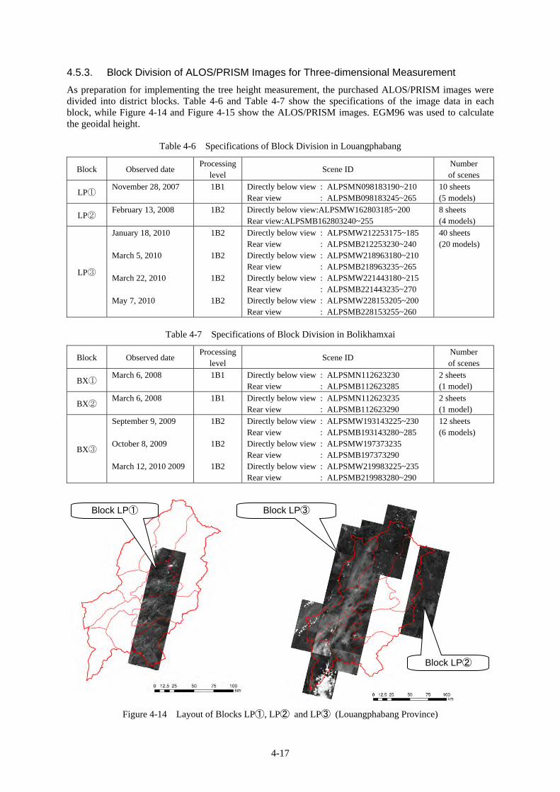
Figure 4-14 Layout of Blocks LP①, LP② and LP③ (Louangphabang Province)

Block LP① Block LP③

Block LP②

4-18

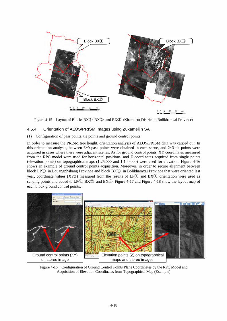
Figure 4-15 Layout of Blocks BX①, BX② and BX③ (Khamkeut District in Bolikhamxai Province) 4.5.4. Orientation of ALOS/PRISM Images using Zukameijin SA

(1) Configuration of pass points, tie points and ground control points

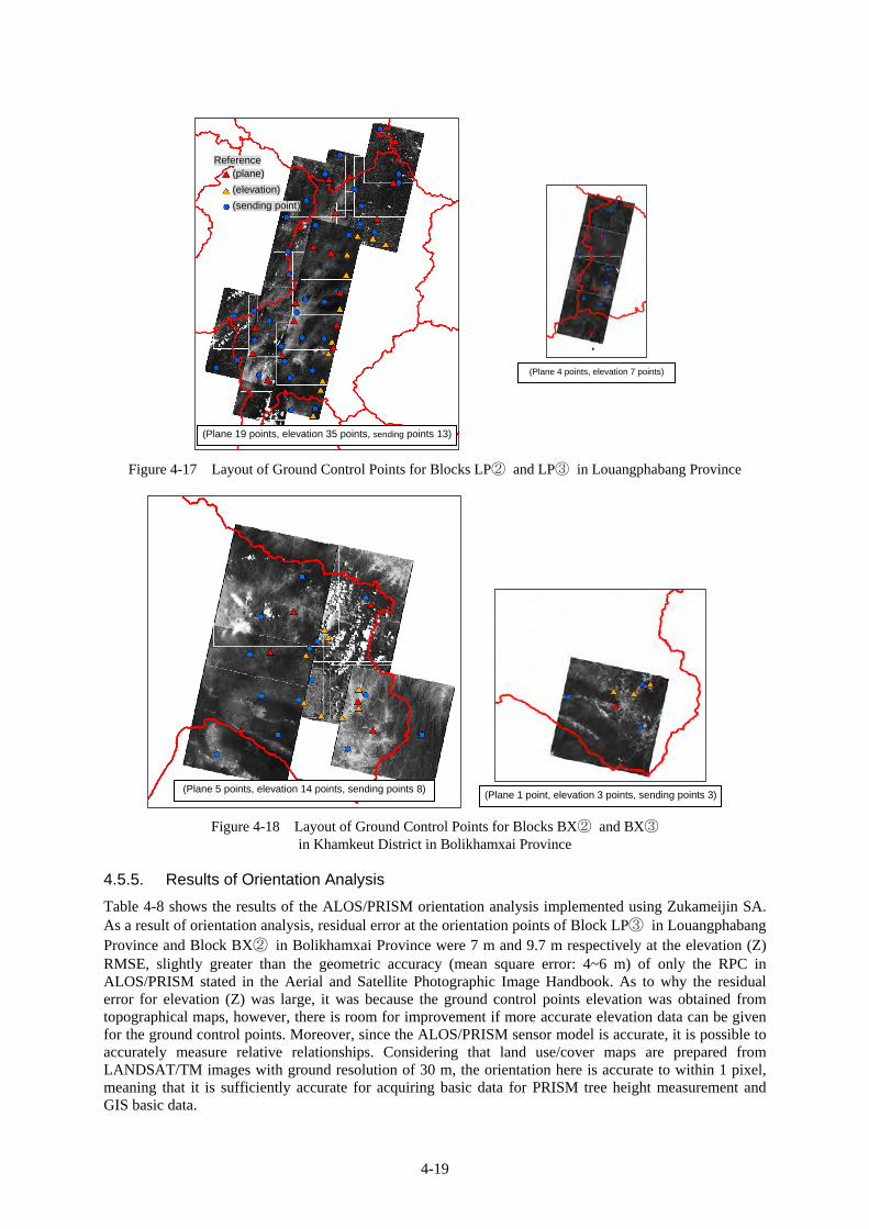
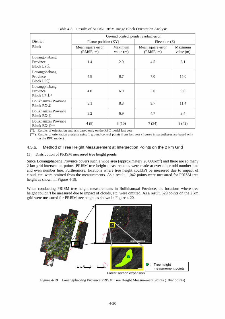
In order to measure the PRISM tree height, orientation analysis of ALOS/PRISM data was carried out. In this orientation analysis, between 6~9 pass points were obtained in each scene, and 2~3 tie points were acquired in cases where there were adjacent scenes. As for ground control points, XY coordinates measured from the RPC model were used for horizontal positions, and Z coordinates acquired from single points (elevation points) on topographical maps (1:25,000 and 1:100,000) were used for elevation. Figure 4-16 shows an example of ground control points acquisition. Moreover, in order to secure alignment between block LP① in Louangphabang Province and block BX① in Bolikhamxai Province that were oriented last year, coordinate values (XYZ) measured from the results of LP① and BX① orientation were used as sending points and added to LP③, BX② and BX③. Figure 4-17 and Figure 4-18 show the layout map of each block ground control points.

Figure 4-16 Configuration of Ground Control Points Plane Coordinates by the RPC Model and Acquisition of Elevation Coordinates from Topographical Map (Example)

Block BX① Block BX③

Block BX②

Ground control points (XY) on stereo image

Elevation points (Z) on topographical maps and stereo images

4-19

Figure 4-17 Layout of Ground Control Points for Blocks LP② and LP③ in Louangphabang Province

Figure 4-18 Layout of Ground Control Points for Blocks BX② and BX③ in Khamkeut District in Bolikhamxai Province

4.5.5. Results of Orientation Analysis

Table 4-8 shows the results of the ALOS/PRISM orientation analysis implemented using Zukameijin SA. As a result of orientation analysis, residual error at the orientation points of Block LP③ in Louangphabang Province and Block BX② in Bolikhamxai Province were 7 m and 9.7 m respectively at the elevation (Z) RMSE, slightly greater than the geometric accuracy (mean square error: 4~6 m) of only the RPC in ALOS/PRISM stated in the Aerial and Satellite Photographic Image Handbook. As to why the residual error for elevation (Z) was large, it was because the ground control points elevation was obtained from topographical maps, however, there is room for improvement if more accurate elevation data can be given for the ground control points. Moreover, since the ALOS/PRISM sensor model is accurate, it is possible to accurately measure relative relationships. Considering that land use/cover maps are prepared from LANDSAT/TM images with ground resolution of 30 m, the orientation here is accurate to within 1 pixel, meaning that it is sufficiently accurate for acquiring basic data for PRISM tree height measurement and GIS basic data.

(Plane 4 points, elevation 7 points)

(plane)

(elevation)

(sending point)

(Plane 19 points, elevation 35 points, sending points 13)

Reference

(Plane 5 points, elevation 14 points, sending points 8)(Plane 1 point, elevation 3 points, sending points 3)

4-20

Table 4-8 Results of ALOS/PRISM Image Block Orientation Analysis

District

Block

Ground control points residual error

Planar position (XY) Elevation (Z)

Mean square error (RMSE, m)

Maximum value (m)

Mean square error (RMSE, m)

Maximum value (m)

Louangphabang Province Block LP②

1.4 2.0 4.5 6.1

Louangphabang Province Block LP③

4.8 8.7 7.0 15.0

Louangphabang Province Block LP①*

4.0 6.0 5.0 9.0

Bolikhamxai Province Block BX②

5.1 8.3 9.7 11.4

Bolikhamxai Province Block BX③

3.2 6.9 4.7 9.4

Bolikhamxai Province Block BX①**

4 (8) 8 (10) 7 (34) 9 (42)

(*): Results of orientation analysis based only on the RPC model last year (**): Results of orientation analysis using 1 ground control points from last year (figures in parentheses are based only

on the RPC model). 4.5.6. Method of Tree Height Measurement at Intersection Points on the 2 km Grid

(1) Distribution of PRISM measured tree height points

Since Louangphabang Province covers such a wide area (approximately 20,000km2) and there are so many 2 km grid intersection points, PRISM tree height measurements were made at ever other odd number line and even number line. Furthermore, locations where tree height couldn’t be measured due to impact of cloud, etc. were omitted from the measurements. As a result, 1,042 points were measured for PRISM tree height as shown in Figure 4-19.

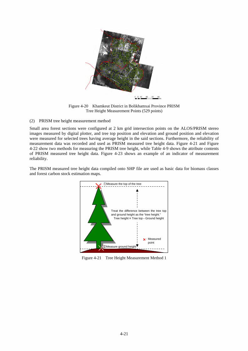
When conducting PRISM tree height measurements in Bolikhamxai Province, the locations where tree height couldn’t be measured due to impact of clouds, etc. were omitted. As a result, 529 points on the 2 km grid were measured for PRISM tree height as shown in Figure 4-20.

Figure 4-19 Louangphabang Province PRISM Tree Height Measurement Points (1042 points)

: Tree height measurement points

Forest section expansion

4-21

Figure 4-20 Khamkeut District in Bolikhamxai Province PRISM Tree Height Measurement Points (529 points)

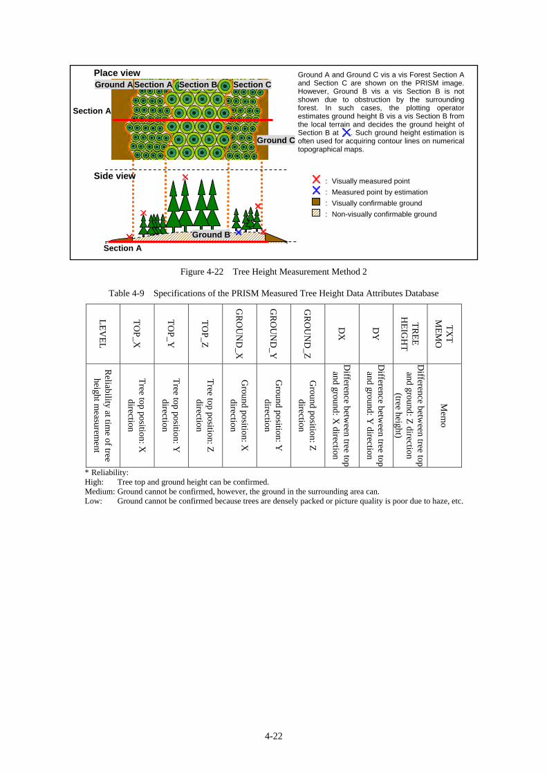
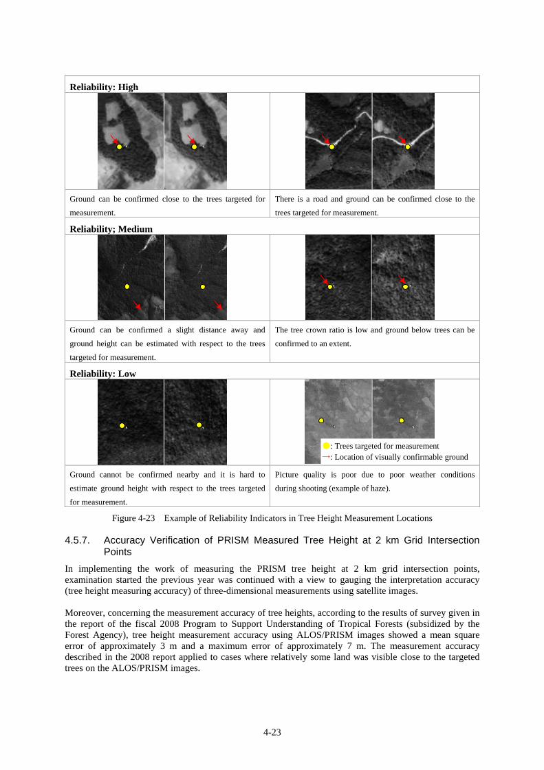
(2) PRISM tree height measurement method

Small area forest sections were configured at 2 km grid intersection points on the ALOS/PRISM stereo images measured by digital plotter, and tree top position and elevation and ground position and elevation were measured for selected trees having average height in the said sections. Furthermore, the reliability of measurement data was recorded and used as PRISM measured tree height data. Figure 4-21 and Figure 4-22 show two methods for measuring the PRISM tree height, while Table 4-9 shows the attribute contents of PRISM measured tree height data. Figure 4-23 shows an example of an indicator of measurement reliability.

The PRISM measured tree height data compiled onto SHP file are used as basic data for biomass classes and forest carbon stock estimation maps.

Figure 4-21 Tree Height Measurement Method 1

①Measure the top of the tree

Treat the difference between the tree top and ground height as the “tree height.”

Tree height = Tree top - Ground height

②Measure ground height

: Measured point

4-22

Figure 4-22 Tree Height Measurement Method 2

Table 4-9 Specifications of the PRISM Measured Tree Height Data Attributes Database

LE

VE

L

TO

P_X

TO

P_Y

TO

P_Z

GR

OU

ND

_X

GR

OU

ND

_Y

GR

OU

ND

_Z

DX

DY

TR

EE

H

EIG

HT

TX

T

ME

MO

Reliability at tim

e of tree height m

easurement

Tree top position: X

direction

Tree top position: Y

direction

Tree top position: Z

direction

Ground position: X

direction

Ground position: Y

direction

Ground position: Z

direction

Difference betw

een tree top and ground: X

direction

Difference betw

een tree top and ground: Y

direction

Difference betw

een tree top and ground: Z

direction (tree height)

Mem

o

* Reliability: High: Tree top and ground height can be confirmed. Medium: Ground cannot be confirmed, however, the ground in the surrounding area can. Low: Ground cannot be confirmed because trees are densely packed or picture quality is poor due to haze, etc.

: Visually measured point

: Measured point by estimation

: Visually confirmable ground

: Non-visually confirmable ground

Ground A and Ground C vis a vis Forest Section Aand Section C are shown on the PRISM image.However, Ground B vis a vis Section B is notshown due to obstruction by the surroundingforest. In such cases, the plotting operatorestimates ground height B vis a vis Section B fromthe local terrain and decides the ground height ofSection B at . Such ground height estimation isoften used for acquiring contour lines on numericaltopographical maps.

Section A Section B Section CGround A Place view

Side view

Ground B

Ground C

Section A

Section A

4-23

Reliability: High

Ground can be confirmed close to the trees targeted for

measurement.

There is a road and ground can be confirmed close to the

trees targeted for measurement.

Reliability; Medium

Ground can be confirmed a slight distance away and

ground height can be estimated with respect to the trees

targeted for measurement.

The tree crown ratio is low and ground below trees can be

confirmed to an extent.

Reliability: Low

Ground cannot be confirmed nearby and it is hard to

estimate ground height with respect to the trees targeted

for measurement.

Picture quality is poor due to poor weather conditions

during shooting (example of haze).

Figure 4-23 Example of Reliability Indicators in Tree Height Measurement Locations 4.5.7. Accuracy Verification of PRISM Measured Tree Height at 2 km Grid Intersection

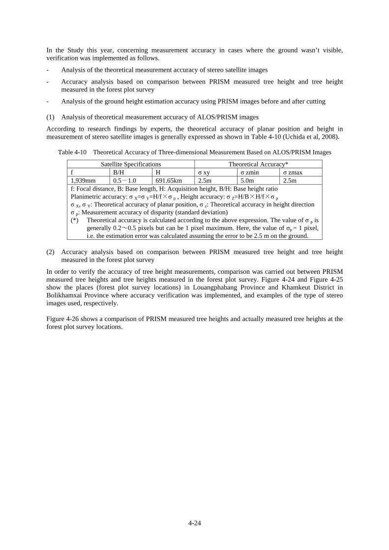
Points

In implementing the work of measuring the PRISM tree height at 2 km grid intersection points, examination started the previous year was continued with a view to gauging the interpretation accuracy (tree height measuring accuracy) of three-dimensional measurements using satellite images.

Moreover, concerning the measurement accuracy of tree heights, according to the results of survey given in the report of the fiscal 2008 Program to Support Understanding of Tropical Forests (subsidized by the Forest Agency), tree height measurement accuracy using ALOS/PRISM images showed a mean square error of approximately 3 m and a maximum error of approximately 7 m. The measurement accuracy described in the 2008 report applied to cases where relatively some land was visible close to the targeted trees on the ALOS/PRISM images.

●: Trees targeted for measurement →: Location of visually confirmable ground

4-24

In the Study this year, concerning measurement accuracy in cases where the ground wasn’t visible, verification was implemented as follows.

- Analysis of the theoretical measurement accuracy of stereo satellite images

- Accuracy analysis based on comparison between PRISM measured tree height and tree height measured in the forest plot survey

- Analysis of the ground height estimation accuracy using PRISM images before and after cutting

(1) Analysis of theoretical measurement accuracy of ALOS/PRISM images

According to research findings by experts, the theoretical accuracy of planar position and height in measurement of stereo satellite images is generally expressed as shown in Table 4-10 (Uchida et al, 2008).

Table 4-10 Theoretical Accuracy of Three-dimensional Measurement Based on ALOS/PRISM Images

Satellite Specifications Theoretical Accuracy* f B/H H σ xy σ zmin σ zmax 1,939mm 0.5－1.0 691.65km 2.5m 5.0m 2.5m f: Focal distance, B: Base length, H: Acquisition height, B/H: Base height ratio Planimetric accuracy: σ X=σ Y=H/f×σ p , Height accuracy: σ Z=H/B×H/f×σ p σ X, σ Y: Theoretical accuracy of planar position, σ z: Theoretical accuracy in height direction σ p: Measurement accuracy of disparity (standard deviation) (*) Theoretical accuracy is calculated according to the above expression. The value of σ p is

generally 0.2～0.5 pixels but can be 1 pixel maximum. Here, the value of σp = 1 pixel, i.e. the estimation error was calculated assuming the error to be 2.5 m on the ground.

(2) Accuracy analysis based on comparison between PRISM measured tree height and tree height

measured in the forest plot survey

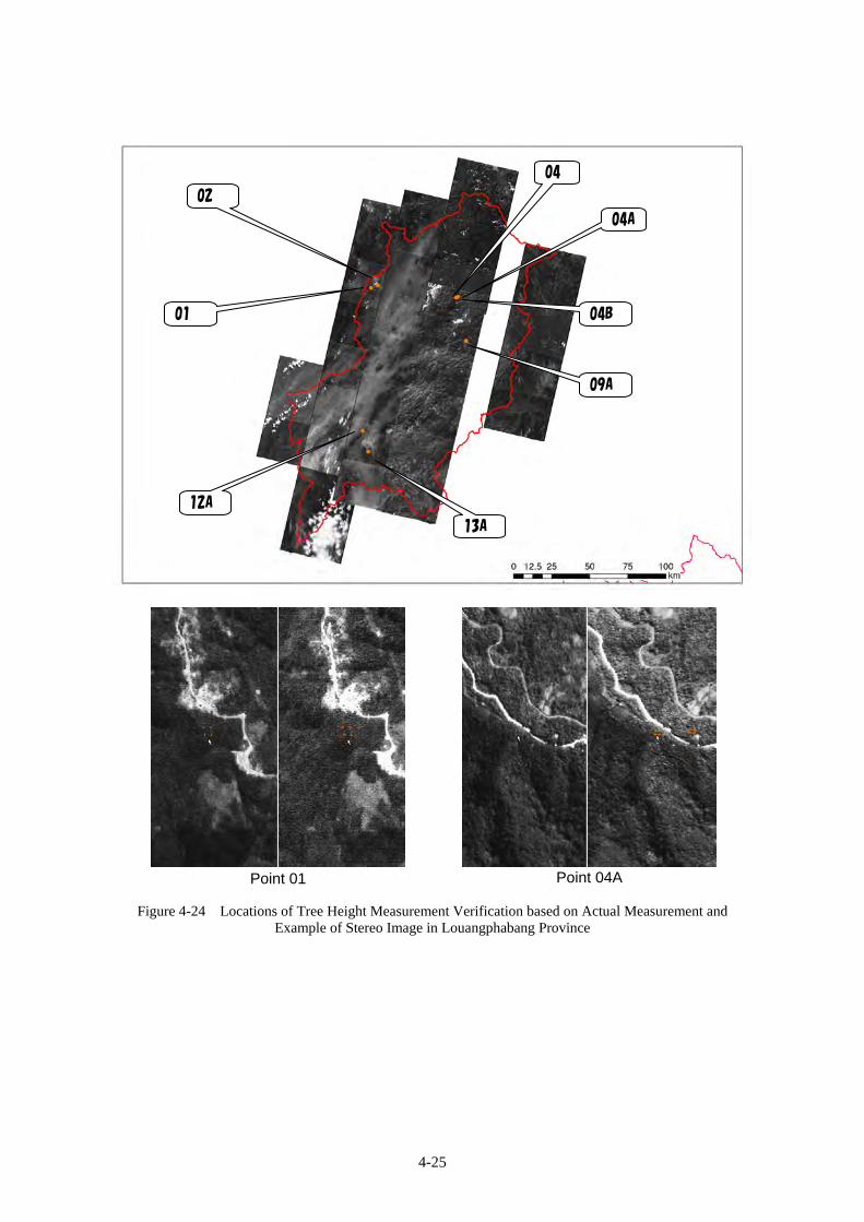
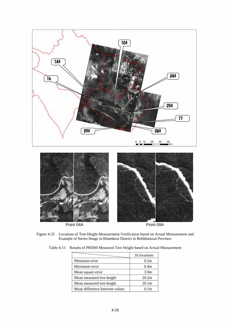
In order to verify the accuracy of tree height measurements, comparison was carried out between PRISM measured tree heights and tree heights measured in the forest plot survey. Figure 4-24 and Figure 4-25 show the places (forest plot survey locations) in Louangphabang Province and Khamkeut District in Bolikhamxai Province where accuracy verification was implemented, and examples of the type of stereo images used, respectively.

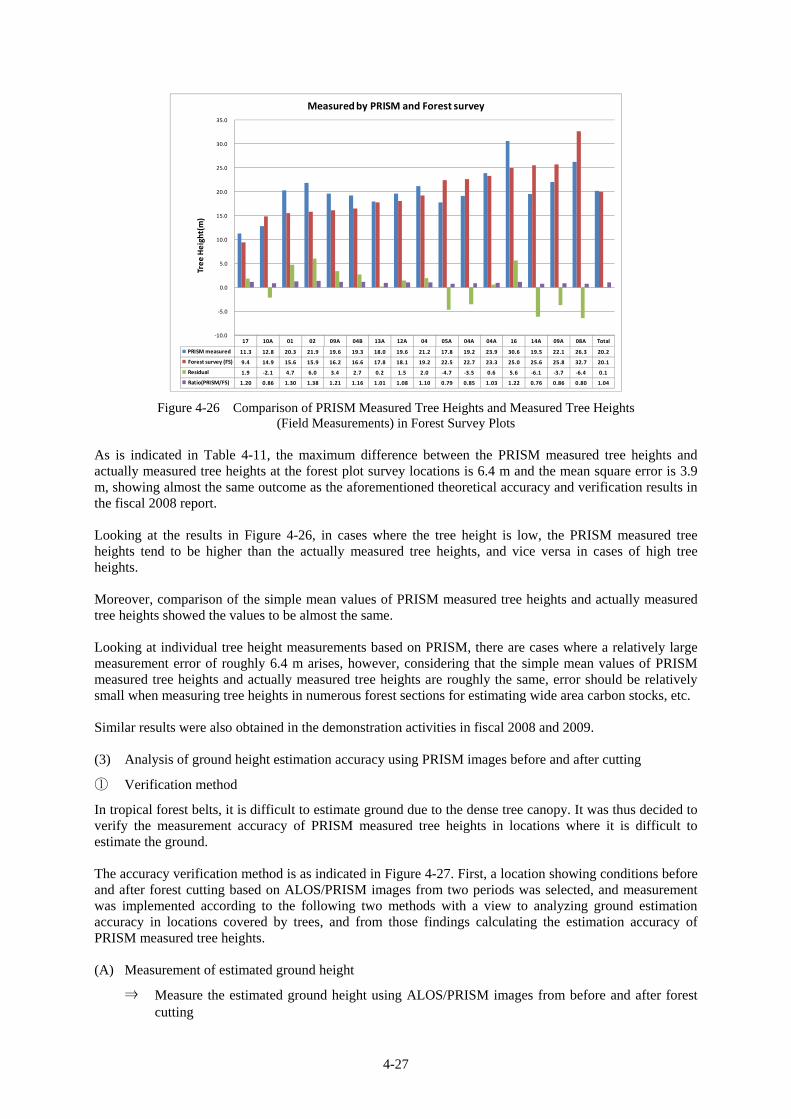
Figure 4-26 shows a comparison of PRISM measured tree heights and actually measured tree heights at the forest plot survey locations.

4-25

Figure 4-24 Locations of Tree Height Measurement Verification based on Actual Measurement and Example of Stereo Image in Louangphabang Province

Point 01 Point 04A

04

04B

09A

13A

12A

01

02

04A

4-26

Figure 4-25 Locations of Tree Height Measurement Verification based on Actual Measurement and Example of Stereo Image in Khamkeut District in Bolikhamxai Province

Table 4-11 Results of PRISM Measured Tree Height based on Actual Measurement

16 locations

Minimum error 0.2m

Maximum error 6.4m

Mean square error 3.9m

Mean measured tree height 20.2m

Mean measured tree height 20.1m

Mean difference between values 0.1m

Point 04A Point 09A

10A

05A

17

08A 09A

16

14A

04A

4-27

17 10A 01 02 09A 04B 13A 12A 04 05A 04A 04A 16 14A 09A 08A Total

PRISM measured 11.3 12.8 20.3 21.9 19.6 19.3 18.0 19.6 21.2 17.8 19.2 23.9 30.6 19.5 22.1 26.3 20.2

Forest survey (FS) 9.4 14.9 15.6 15.9 16.2 16.6 17.8 18.1 19.2 22.5 22.7 23.3 25.0 25.6 25.8 32.7 20.1

Residual 1.9 ‐2.1 4.7 6.0 3.4 2.7 0.2 1.5 2.0 ‐4.7 ‐3.5 0.6 5.6 ‐6.1 ‐3.7 ‐6.4 0.1

Ratio(PRISM/FS) 1.20 0.86 1.30 1.38 1.21 1.16 1.01 1.08 1.10 0.79 0.85 1.03 1.22 0.76 0.86 0.80 1.04

‐10.0

‐5.0

0.0

5.0

10.0

15.0

20.0

25.0

30.0

35.0

Tree Height(m)

Measured by PRISM and Forest survey

Figure 4-26 Comparison of PRISM Measured Tree Heights and Measured Tree Heights (Field Measurements) in Forest Survey Plots

As is indicated in Table 4-11, the maximum difference between the PRISM measured tree heights and actually measured tree heights at the forest plot survey locations is 6.4 m and the mean square error is 3.9 m, showing almost the same outcome as the aforementioned theoretical accuracy and verification results in the fiscal 2008 report.

Looking at the results in Figure 4-26, in cases where the tree height is low, the PRISM measured tree heights tend to be higher than the actually measured tree heights, and vice versa in cases of high tree heights.

Moreover, comparison of the simple mean values of PRISM measured tree heights and actually measured tree heights showed the values to be almost the same.

Looking at individual tree height measurements based on PRISM, there are cases where a relatively large measurement error of roughly 6.4 m arises, however, considering that the simple mean values of PRISM measured tree heights and actually measured tree heights are roughly the same, error should be relatively small when measuring tree heights in numerous forest sections for estimating wide area carbon stocks, etc.

Similar results were also obtained in the demonstration activities in fiscal 2008 and 2009.

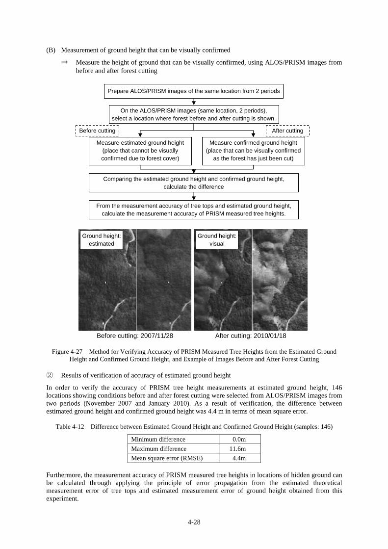
(3) Analysis of ground height estimation accuracy using PRISM images before and after cutting

① Verification method

In tropical forest belts, it is difficult to estimate ground due to the dense tree canopy. It was thus decided to verify the measurement accuracy of PRISM measured tree heights in locations where it is difficult to estimate the ground.

The accuracy verification method is as indicated in Figure 4-27. First, a location showing conditions before and after forest cutting based on ALOS/PRISM images from two periods was selected, and measurement was implemented according to the following two methods with a view to analyzing ground estimation accuracy in locations covered by trees, and from those findings calculating the estimation accuracy of PRISM measured tree heights.

(A) Measurement of estimated ground height

⇒ Measure the estimated ground height using ALOS/PRISM images from before and after forest cutting

4-28

(B) Measurement of ground height that can be visually confirmed

⇒ Measure the height of ground that can be visually confirmed, using ALOS/PRISM images from before and after forest cutting

Figure 4-27 Method for Verifying Accuracy of PRISM Measured Tree Heights from the Estimated Ground Height and Confirmed Ground Height, and Example of Images Before and After Forest Cutting

② Results of verification of accuracy of estimated ground height

In order to verify the accuracy of PRISM tree height measurements at estimated ground height, 146 locations showing conditions before and after forest cutting were selected from ALOS/PRISM images from two periods (November 2007 and January 2010). As a result of verification, the difference between estimated ground height and confirmed ground height was 4.4 m in terms of mean square error.

Table 4-12 Difference between Estimated Ground Height and Confirmed Ground Height (samples: 146)

Minimum difference 0.0m

Maximum difference 11.6m

Mean square error (RMSE) 4.4m Furthermore, the measurement accuracy of PRISM measured tree heights in locations of hidden ground can be calculated through applying the principle of error propagation from the estimated theoretical measurement error of tree tops and estimated measurement error of ground height obtained from this experiment.

Before cutting: 2007/11/28 After cutting: 2010/01/18

Ground height: estimated

Ground height: visual

Prepare ALOS/PRISM images of the same location from 2 periods

On the ALOS/PRISM images (same location, 2 periods), select a location where forest before and after cutting is shown.

Measure estimated ground height (place that cannot be visually confirmed due to forest cover)

Comparing the estimated ground height and confirmed ground height, calculate the difference

From the measurement accuracy of tree tops and estimated ground height, calculate the measurement accuracy of PRISM measured tree heights.

Measure confirmed ground height (place that can be visually confirmed

as the forest has just been cut)

Before cutting After cutting

4-29

Tree height measurement error (RMSE) when estimating ground height = SQRT (tree top theoretical measurement error＾2 + ground estimation error＾2) = SQRT（4.4＾2+2.5＾2）=5.1m

Here, the theoretical error of tree top is assumed to be the theoretical accuracy (0.5 pixels) in the PRISM height direction.

③ Relationship between terrain and tree height measurement accuracy

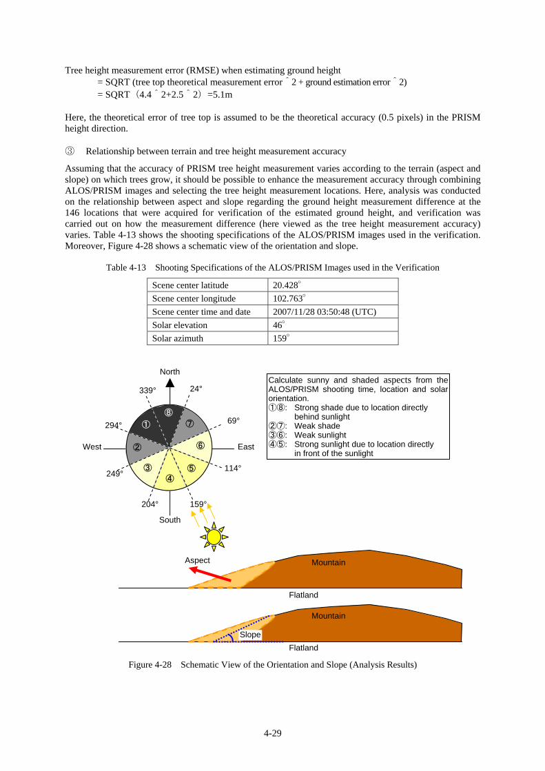
Assuming that the accuracy of PRISM tree height measurement varies according to the terrain (aspect and slope) on which trees grow, it should be possible to enhance the measurement accuracy through combining ALOS/PRISM images and selecting the tree height measurement locations. Here, analysis was conducted on the relationship between aspect and slope regarding the ground height measurement difference at the 146 locations that were acquired for verification of the estimated ground height, and verification was carried out on how the measurement difference (here viewed as the tree height measurement accuracy) varies. Table 4-13 shows the shooting specifications of the ALOS/PRISM images used in the verification. Moreover, Figure 4-28 shows a schematic view of the orientation and slope.

Table 4-13 Shooting Specifications of the ALOS/PRISM Images used in the Verification

Scene center latitude 20.428°

Scene center longitude 102.763°

Scene center time and date 2007/11/28 03:50:48 (UTC)

Solar elevation 46°

Solar azimuth 159°

Figure 4-28 Schematic View of the Orientation and Slope (Analysis Results)

Flatland

Aspect

Slope

Mountain

Mountain

Flatland

24°

204°

249°

North

East

South

West ②

③ ④

⑤

⑥

⑦ ⑧

①

339°

69°

114°

159°

294°

Calculate sunny and shaded aspects from the ALOS/PRISM shooting time, location and solar orientation. ①⑧: Strong shade due to location directly

behind sunlight ②⑦: Weak shade ③⑥: Weak sunlight ④⑤: Strong sunlight due to location directly

in front of the sunlight

4-30

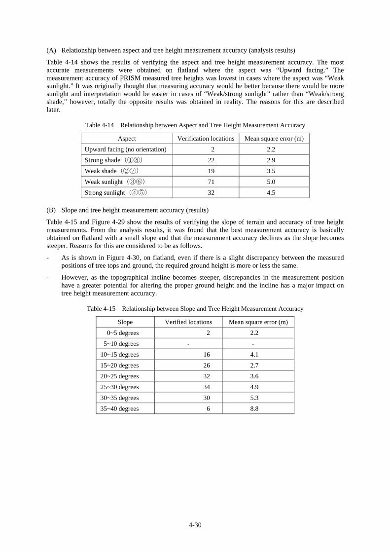
(A) Relationship between aspect and tree height measurement accuracy (analysis results)

Table 4-14 shows the results of verifying the aspect and tree height measurement accuracy. The most accurate measurements were obtained on flatland where the aspect was “Upward facing.” The measurement accuracy of PRISM measured tree heights was lowest in cases where the aspect was “Weak sunlight.” It was originally thought that measuring accuracy would be better because there would be more sunlight and interpretation would be easier in cases of “Weak/strong sunlight” rather than “Weak/strong shade,” however, totally the opposite results was obtained in reality. The reasons for this are described later.

Table 4-14 Relationship between Aspect and Tree Height Measurement Accuracy

Aspect Verification locations Mean square error (m)

Upward facing (no orientation) 2 2.2

Strong shade（①⑧） 22 2.9

Weak shade（②⑦） 19 3.5

Weak sunlight（③⑥） 71 5.0

Strong sunlight（④⑤） 32 4.5

(B) Slope and tree height measurement accuracy (results)

Table 4-15 and Figure 4-29 show the results of verifying the slope of terrain and accuracy of tree height measurements. From the analysis results, it was found that the best measurement accuracy is basically obtained on flatland with a small slope and that the measurement accuracy declines as the slope becomes steeper. Reasons for this are considered to be as follows.

- As is shown in Figure 4-30, on flatland, even if there is a slight discrepancy between the measured positions of tree tops and ground, the required ground height is more or less the same.

- However, as the topographical incline becomes steeper, discrepancies in the measurement position have a greater potential for altering the proper ground height and the incline has a major impact on tree height measurement accuracy.

Table 4-15 Relationship between Slope and Tree Height Measurement Accuracy

Slope Verified locations Mean square error (m)

0~5 degrees 2 2.2

5~10 degrees - -

10~15 degrees 16 4.1

15~20 degrees 26 2.7

20~25 degrees 32 3.6

25~30 degrees 34 4.9

30~35 degrees 30 5.3

35~40 degrees 6 8.8

4-31

0～5° 5～10° 10～15° 15～20° 20～25° 25～30° 30～35° 35～40°

Mean square error (m) 2.2 4.1 2.7 3.6 4.9 5.3 8.8

0.0

1.0

2.0

3.0

4.0

5.0

6.0

7.0

8.0

9.0

10.0

Mean

square error (m)

Angle of incline

Figure 4-29 Relationship between Slope and Tree Height Measurement Accuracy

Figure 4-30 Comparison of Ground Estimation Error between Flatland and Steep Incline (C) Terrain and tree height measurement accuracy (results)

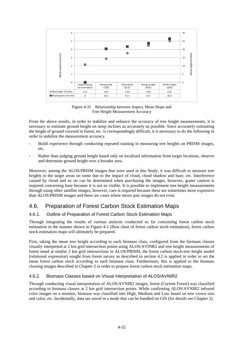
As a result of analyzing the relationship between slope of terrain and tree height measurement accuracy, it was found that the measurement accuracy deteriorates when the slope becomes steep. Table 4-16 shows the relationships between aspect, mean slope and error. From these results, it can be seen that the accuracy of tree height measurement is dependent on the slope, irrespective of the aspect (See Figure 4-31).

Table 4-16 Relationship between Aspect, Mean Slope and PRISM Tree Height Measurement Accuracy

Aspect Verified locations

Mean slope Mean square error (m)

Upward facing (no orientation) 2 0° 2.2

Strong shade（①⑧） 22 20.3° 2.9

Weak shade（②⑦） 19 21.7° 3.5

Strong sunlight（④⑤） 32 23.7° 4.5

Weak sunlight（③⑥） 71 26.4° 5.0

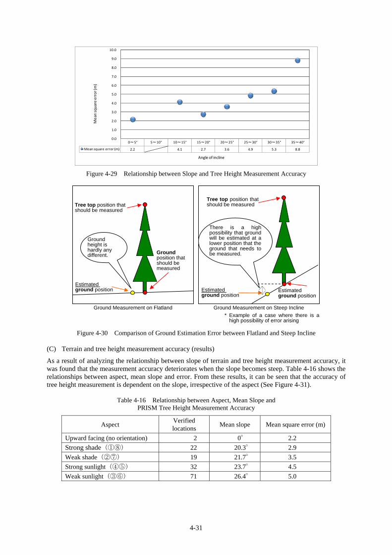
Tree top position that should be measured

Ground position that should be measured

Estimated ground position

Ground height is hardly any different.

Tree top position thatshould be measured



There is a high possibility that ground will be estimated at a lower position that the ground that needs to be measured.

Ground Measurement on Flatland Ground Measurement on Steep Incline

* Example of a case where there is ahigh possibility of error arising

4-32

Upward facing (no orientation)

Strong shade

（①⑧）

Weak shade

（②⑦）

Strong sunlight

（④⑤）

Weak sunlight

（③⑥）

Mean angle of incline 2.15 2.87 3.54 4.48 5.02

Mean square error (m) 0 20.3 21.7 23.7 26.4

0

5

10

15

20

25

30

0

1

2

3

4

5

6

Mean

square error (m)

Mean

angle of incline

Figure 4-31 Relationship between Aspect, Mean Slope and Tree Height Measurement Accuracy

From the above results, in order to stabilize and enhance the accuracy of tree height measurements, it is necessary to estimate ground height on steep inclines as accurately as possible. Since accurately estimating the height of ground covered in forest, etc. is correspondingly difficult, it is necessary to do the following in order to stabilize the measurement accuracy.

- Build experience through conducting repeated training in measuring tree heights on PRISM images, etc.

- Rather than judging ground height based only on localized information from target locations, observe and determine ground height over a broader area.

Moreover, among the ALOS/PRISM images that were used in this Study, it was difficult to measure tree heights in the target areas on some due to the impact of cloud, cloud shadow and haze, etc. Interference caused by cloud and so on can be determined when purchasing the images, however, grater caution is required concerning haze because it is not so visible. It is possible to implement tree height measurements through using other satellite images, however, care is required because these are sometimes more expensive than ALOS/PRISM images and there are cases where stereo pair images do not exist.

4.6. Preparation of Forest Carbon Stock Estimation Maps 4.6.1. Outline of Preparation of Forest Carbon Stock Estimation Maps

Through integrating the results of various analysis conducted so far concerning forest carbon stock estimation in the manner shown in Figure 4-1 (flow chart of forest carbon stock estimation), forest carbon stock estimation maps will ultimately be prepared.

First, taking the mean tree height according to each biomass class, configured from the biomass classes visually interpreted at 2 km grid intersection points using ALOS/AVINR2 and tree height measurements of forest stand at similar 2 km grid intersections in ALOS/PRISM, the forest carbon stock-tree height model (relational expression) sought from forest survey as described in section 4.2 is applied in order to set the mean forest carbon stock according to each biomass class. Furthermore, this is applied to the biomass classing images described in Chapter 2 in order to prepare forest carbon stock estimation maps.

4.6.2. Biomass Classes based on Visual Interpretation of ALOS/AVNIR2

Through conducting visual interpretation of ALOS/AVNIR2 images, forest (Current Forest) was classified according to biomass classes at 2 km grid intersection points. While confirming ALOS/AVNIR2 infrared color images on a monitor, biomass was classified into High, Medium and Low based on tree crown size and color, etc. Incidentally, data are saved in a mode that can be handled on GIS (for details see Chapter 2).

4-33

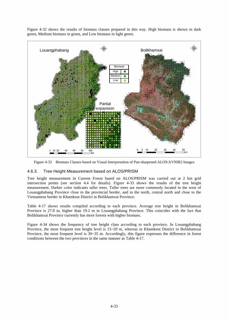
Figure 4-32 shows the results of biomass classes prepared in this way. High biomass is shown in dark green, Medium biomass in green, and Low biomass in light green.

Figure 4-32 Biomass Classes based on Visual Interpretation of Pan-sharpened ALOS/AVNIR2 Images 4.6.3. Tree Height Measurement based on ALOS/PRISM

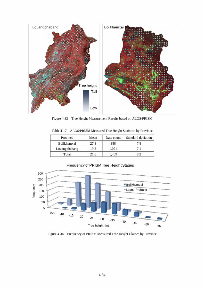
Tree height measurement in Current Forest based on ALOS/PRISM was carried out at 2 km grid intersection points (see section 4.4 for details). Figure 4-33 shows the results of the tree height measurement. Darker color indicates taller trees. Taller trees are more commonly located in the west of Louangphabang Province close to the provincial border, and in the north, central north and close to the Vietnamese border in Khamkeut District in Bolikhamxai Province.

Table 4-17 shows results compiled according to each province. Average tree height in Bolikhamxai Province is 27.8 m, higher than 19.2 m in Louangphabang Province. This coincides with the fact that Bolikhamxai Province currently has more forests with higher biomass.

Figure 4-34 shows the frequency of tree height class according to each province. In Louangphabang Province, the most frequent tree height level is 15~20 m, whereas in Khamkeut District in Bolikhamxai Province, the most frequent level is 30~35 m. Accordingly, this figure expresses the difference in forest conditions between the two provinces in the same manner as Table 4-17.


Partial expansion

Biomass

High

Medium

Low

4-34

Figure 4-33 Tree Height Measurement Results based on ALOS/PRISM

Table 4-17 ALOS/PRISM Measured Tree Height Statistics by Province

Province Mean Data count Standard deviation

Bolikhamxai 27.8 388 7.8

Louangphabang 19.2 1,021 7.1

Total 21.6 1,409 8.2

0

50

100

150

200

250

300

0-5 -10 -15 -20 -25 -30 -35 -40 -45 -50 -55

Fre

que

ncy

Tree height (m)

Frequency of PRISM Tree Height Stages

Bolikhamsai

Luang Prabang

Figure 4-34 Frequency of PRISM Measured Tree Height Classes by Province


Tree height

Tall

Low

4-35

4.6.4. Setting of Mean Tree Heights according to Biomass Class

In view of the high correlation between biomass and tree heights, the results of biomass classing based on ALOS/AVNIR2 (4.6.2) and tree height measurements based on ALOS/PRISM (4.6.3) were aggregated in order to seek the mean tree height according to each biomass class.

The resulting values were configured as the mean tree heights for each biomass class (see Table 4-18 and Figure 4-35). Although the standard deviation in each class is high and there is some overlapping between classes, the mean, median and most frequent values of PRISM tree height increase as the biomass class moves from Low to Medium to High, indicating a positive relationship between the two items.

Table 4-18 Mean Tree Height According to Biomass Class

Biomass class Tree height (PRISM measurement)

(AVNIR2 interpretation)

Mean Standard deviation

Number of trees

Minimum Maximum Median Most

frequent value

High 26.8 5.2 138 17.2 37.3 25.7 30.3

Medium 24.1 6.1 286 8.3 35.5 23.7 23.3

Low 18.4 4.8 588 1.7 27.4 18.6 16.3

Total 21.2 6.2 1012 1.7 37.3 21.0 21.0

High, 26.8

Medium, 24.1

Low, 18.4

10.0

15.0

20.0

25.0

30.0

35.0

PR

ISM

Mea

sure

d T

ree

Hei

ght

(m

)

AVNIR2 Interpreted Biomass Class

Figure 4-35 Mean Tree Height According to Biomass Class 4.6.5. Setting of Mean Forest Carbon Stock according to Biomass Class

The mean forest carbon stock according to each biomass class was configured upon applying the mean tree heights according to biomass class to the model expression of forest carbon stock-tree height that was configured in section 4.3 (see Table 4-1).

The right column in the table shows the results of forest survey. Although the small number of forest survey locations with respect to the PRISM measured locations means that no conclusive statement can be made, there is a trend whereby tree height increases as the biomass class rises. Moreover, there are no major discrepancies in the tree heights and forest carbon stock values. However, considering the current conditions of forest in Louangphabang Province and Bolikhamxai Province and taking into account the fact that tree height of 5 m or higher is defined as Current Forest in Lao PDR, the figure of 18.4 m in the Low biomass class is rather high.

4-36

Table 4-19 Mean Forest Carbon Stock according to Biomass Class

Biomass class

PRISM measurement Forest survey

Tree height (m)

Forest carbon stock (Tc/ha)

Number of trees

Tree height (m)

Forest carbon stock (Tc/ha)

Number of trees

High 26.8 404.4 138 29.2 506.1 4

Medium 24.1 306.6 286 21.9 235.1 6

Low 18.4 155.3 588 16.0 137.7 11

Total 21.2 221.1 1012 20.2 235.7 21 4.6.6. Preparation of Forest Carbon Stock Estimation Maps

Through applying the biomass class-separate mean forest carbon stocks to the biomass classing maps prepared in Chapter 2, forest carbon stock estimation maps were prepared. Moreover, concerning Louangphabang Province, since the classification accuracy of the biomass classing map is low at 60 percent or less, it was decided to only prepare the map for Khamkeut District in Bolikhamxai Province, where classification accuracy is 60 percent or higher.

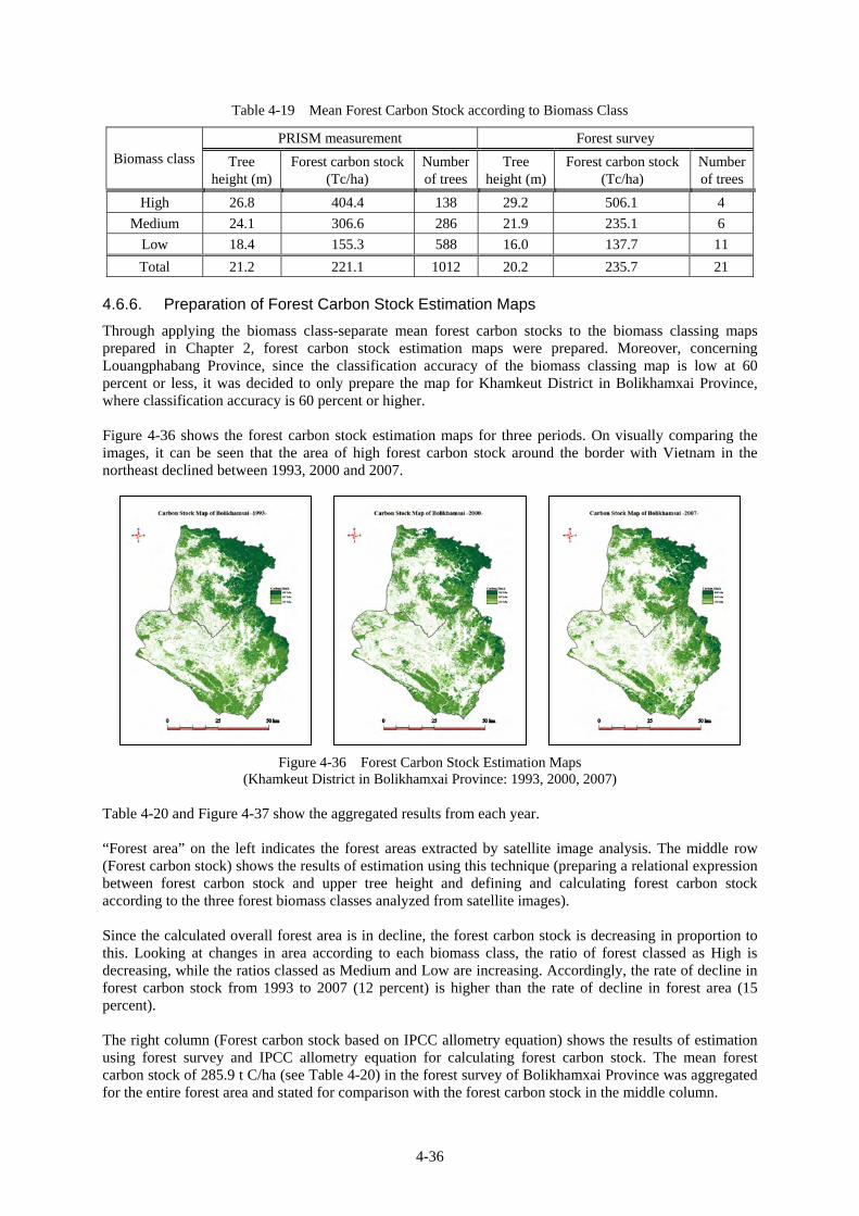
Figure 4-36 shows the forest carbon stock estimation maps for three periods. On visually comparing the images, it can be seen that the area of high forest carbon stock around the border with Vietnam in the northeast declined between 1993, 2000 and 2007.

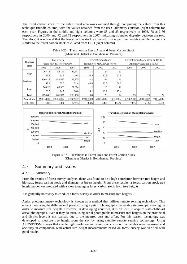
Figure 4-36 Forest Carbon Stock Estimation Maps (Khamkeut District in Bolikhamxai Province: 1993, 2000, 2007)

Table 4-20 and Figure 4-37 show the aggregated results from each year.

“Forest area” on the left indicates the forest areas extracted by satellite image analysis. The middle row (Forest carbon stock) shows the results of estimation using this technique (preparing a relational expression between forest carbon stock and upper tree height and defining and calculating forest carbon stock according to the three forest biomass classes analyzed from satellite images).

Since the calculated overall forest area is in decline, the forest carbon stock is decreasing in proportion to this. Looking at changes in area according to each biomass class, the ratio of forest classed as High is decreasing, while the ratios classed as Medium and Low are increasing. Accordingly, the rate of decline in forest carbon stock from 1993 to 2007 (12 percent) is higher than the rate of decline in forest area (15 percent).

The right column (Forest carbon stock based on IPCC allometry equation) shows the results of estimation using forest survey and IPCC allometry equation for calculating forest carbon stock. The mean forest carbon stock of 285.9 t C/ha (see Table 4-20) in the forest survey of Bolikhamxai Province was aggregated for the entire forest area and stated for comparison with the forest carbon stock in the middle column.

4-37

The forest carbon stock for the entire forest area was examined through comprising the values from this technique (middle column) with the values obtained from the IPCC allometry equation (right column) for each year. Figures in the middle and right columns were 85 and 83 respectively in 1993, 78 and 76 respectively in 2000, and 72 and 72 respectively in 2007, indicating no major disparity between the two. Therefore, it was found that the forest carbon stock estimated from upper tree heights (middle column) is similar to the forest carbon stock calculated from DBH (right column).

Table 4-20 Transitions in Forest Area and Forest Carbon Stock (Khamkeut District in Bolikhamxai Province)

Biomass

class

Forest Area

(upper row: ha, lower row: %)

Forest Carbon Stock

(upper row: Mt C, lower row:%)

Forest Carbon Stock based on IPCC

Allometry Equation ( Mt C)

1993 2000 2007 1993 2000 2007 1993 2000 2007

High 76,414 58,196 49,541 31 24 20

26.4 21.8 19.5 36.5 30.3 27.9

Medium 136,412 142,817 132,875 42 44 41

47.1 53.5 52.4 49.4 56.5 56.7

Low 76,820 65,963 71,074 12 10 11

26.5 24.7 28.0 14.1 13.2 15.4

Total 289,646 266,976 253,490 85 78 72 83 76 72

Annual rate

of decline

1993-2000 2000-2007 1993-2007 1993-2000 2000-2007 1993-2007 1993-2000 2000-2007 1993-2007

7.8% 5.1% 12.5% 8.4% 7.4% 15.2% 7.8% 5.1% 12.5%

Heigh

Medium

Low

total

0

50,000

100,000

150,000

200,000

250,000

300,000

350,000

1993 2000 2007

Ha

Transitions in Forest Area (Bolikhamsai)

Heigh

Medium

Low

total

0

20

40

60

80

100

1993 2000 2007

Mt C

Transitions in Carbon Stock (Bolikhamsai)

Figure 4-37 Transitions in Forest Area and Forest Carbon Stock (Khamkeut District in Bolikhamxai Province)

4.7. Summary and Issues 4.7.1. Summary

From the results of forest survey analysis, there was found to be a high correlation between tree height and biomass, forest carbon stock and diameter at breast height. From these results, a forest carbon stock-tree height model was prepared with a view to gauging forest carbon stock from tree heights.

It is generally necessary to conduct a forest survey in order to measure tree heights.

Aerial photogrammetry technology is known as a method that utilizes remote sensing technology. This entails measuring the difference of parallax using a pair of photographs that enable stereoscopic viewing, in order to measure tree heights. However, in developing countries, it is difficult to acquire state-of-the-art aerial photographs. Even if they do exist, using aerial photographs to measure tree heights on the provincial and district levels is not realistic due to the incurred cost and effort. For this reason, technology was developed to measure tree height from the sky by using satellite remote sensing technology. Using ALOS/PRISM images that enable high resolution and stereoscopic vision, tree heights were measured and accuracy in comparison with actual tree height measurements based on forest survey was verified with good results.

4-38

As a method for measuring tree heights over an entire province, 2 km grid intersections were set and a sampling method entailing measurement of mean tree height of forest stand at these intersection points was adopted. This technique can efficiently measure tree heights over a wide scope and is effective for conducting forest analysis on the provincial level.

Next, analysis using medium resolution satellite images was carried out in order to extend this approach to the wall-to-wall area. Focusing on the fact that there is high correlation between satellite image and forest factors especially biomass and tree height, forests were finely classified according to biomass. It was possible to divide forests into three biomass classes in spite of the impact exerted by the quality of used satellite images.

Since there is also a high correlation between biomass and tree height, mean tree heights according to each biomass class were set and applied to the forest carbon stock-tree height model in order to obtain the mean forest carbon stock according to each biomass class and prepare wall-to-wall forest carbon stock estimation maps.

4.7.2. Issues

The results of forest survey are used in preparing the forest carbon stock-tree height model. Almost all the forests targeted in this Study were the evergreen broad-leaved type, however, various other forest types (deciduous broad-leaved forest, conifer forest and mixed forest) exist in other areas. Therefore, although this model can be applied to the target areas of the Study, it will be necessary to implement unique forest surveys in order to create models applicable to other areas.

Caution is also required concerning the tree crown density of forests. The areas targeted by the forest survey here were almost all dense forest stands. However, since multiple layer forests exist in other areas, it will be necessary to conduct forest survey and prepare forest carbon stock-tree height models corresponding to each forest stand profile in addition to the abovementioned area-separate forest survey.

Expectations are placed on tree height measurement based on ALOS/PRISM as an alternative technology to tree height measurement based on forest survey and aerial photography. However, it is necessary to conduct training in order to impart technology and it is essential to have knowledge concerning forests and aerial photogrammetry. Having said that, it is not as difficult as satellite remote sensing analysis (for example, automatic classification of land use), which requires expert knowledge and trial and error in order to enhance accuracy.

Concerning satellite images, even if images are the same type and are taken in the same location, appearance varies depending on the season, time of day and atmospheric conditions. In other words, even images showing the same location and same land cover can have different spectral characteristics. However, this is a condition for satellite images that have been used. In order to make this technique more certain, it is necessary to carry out similar verification in different locations and at different times.

Documents

4. TECHNOLOGY DEVELOPMENT FOR ESTIMATING ......4-1 4. Technology Development for Estimating Forest Carbon Stocks 4.1. Outline of Technology Development for Gauging Forest Carbon Stocks