42 GEOMETRIC INTERSECTION

42 GEOMETRIC INTERSECTION

David M. Mount

INTRODUCTION

Detecting whether two geometric objects intersect and computing the region ofintersection are fundamental problems in computational geometry. Geometric in-tersection problems arise naturally in a number of applications. Examples includegeometric packing and covering, wire and component layout in VLSI, map overlayin geographic information systems, motion planning, and collision detection. Insolid modeling, computing the volume of intersection of two shapes is an importantstep in defining complex solids. In computer graphics, detecting the objects thatoverlap a viewing window is an example of an intersection problem, as is computingthe first intersection of a ray and a collection of geometric solids.

Intersection problems are fundamental to many aspects of geometric comput-ing. It is beyond the scope of this chapter to completely survey this area. Insteadwe illustrate a number of the principal techniques used in efficient intersectionalgorithms. This chapter is organized as follows. Section 42.1 discusses intersec-tion primitives, the low-level issues of computing intersections that are commonto high-level algorithms. Section 42.2 discusses detecting the existence of intersec-tions. Section 42.3 focuses on issues related to counting the number of intersectionsand reporting intersections. Section 42.4 deals with problems related to construct-ing the actual region of intersection. Section 42.5 considers methods for geometricintersections based on spatial subdivisions.

42.1 INTERSECTION PREDICATES

GLOSSARY

Geometric predicate: A function that computes a discrete relationship be-tween basic geometric objects.

Boundary elements: The vertices, edges, and faces of various dimensions thatmake up the boundary of an object.

Complex geometric objects are typically constructed from a number of primitiveobjects. Intersection algorithms that operate on complex objects often work bybreaking the problem into a series of primitive geometric predicates acting on basicelements, such as points, lines and curves, that form the boundary of the objectsinvolved. Examples of geometric predicates include determining whether two linesegments intersect each other or whether a point lies above, below, or on a given line.Computing these predicates can be reduced to computing the sign of a polynomial,ideally of low degree. In many instances the polynomial arises as the determinantof a symbolic matrix.

1113

Preliminary version (July 20, 2017). To appear in the Handbook of Discrete and Computational Geometry,J.E. Goodman, J. O'Rourke, and C. D. Tóth (editors), 3rd edition, CRC Press, Boca Raton, FL, 2017.

1114 David M. Mount

Computing geometric predicates in a manner that is efficient, accurate, androbust can be quite challenging. Floating-point computations are fast but sufferfrom round-off errors, which can result in erroneous decisions. These errors inturn can lead to topological inconsistencies in object representations, and theseinconsistencies can cause the run-time failures. Some of the approaches used toaddress robustness in geometric predicates include approximation algorithm thatare robust to floating-point errors [SI94], computing geometric predicates exactlyusing adaptive floating-point arithmetic [Cla92, ABD+97], exact arithmetic com-bined with fast floating-point filters [BKM+95, FW96], and designing algorithmsthat are based on a restricted set of geometric predicates [BS00, BV02].

When the points of intersection are themselves used to as inputs in the construc-tion of other discrete geometric structures, they are typically first rounded to finiteprecision. The rounding process needs to be performed with care, for otherwisetopological inconsistencies may result. Snap rounding is a method for convertingan arrangement of line segments in the plane into a fixed-precision representationby rounding segment intersection points to the vertices of a square grid [Hob99](see also [GY86]). Various methods have been proposed and analyzed for imple-menting this concept (see, e.g., [HP02, BHO07, Her13]). For further information,see Chapter 28.

We will concentrate on geometric intersections involving flat objects (line seg-ments, polygons, polyhedra), but there is considerable interest in computing inter-sections of curves and surfaces (see, e.g., [AKO93, APS93, BO79, CEGS91, JG91,LP79b]). Predicates for curve and surface intersections are particularly challenging,because the intersection of surfaces of a given algebraic degree generally results in acurve of a significantly higher degree. Computing intersection primitives typicallyinvolves solving an algebraic system equations, which can be performed either ex-actly by algebraic and symbolic methods [Yap93] or approximately by numericalmethods [Hof89, MC91]. See Chapter 45.

42.2 INTERSECTION DETECTION

GLOSSARY

Polygonal chain: A sequence of line segments joined end-to-end.

Self-intersecting: Said of a polygonal chain if any pair of nonadjacent edgesintersects one another.

Bounding box: A rectangular box surrounding an object, usually axis-aligned(isothetic).

Intersection detection, the easiest of all intersection tasks, requires merely de-termining the existence of an intersection. Nonetheless, detecting intersections effi-ciently in the absence of simplifying geometric structure can be challenging. As anexample, consider the following fundamental intersection problem, posed by JohnHopcroft in the early 1980s. Given a set of n points and n lines in the plane, does anypoint lie on any line? A series of efforts to solve Hopcroft’s problem culminatedin the best algorithm known for this problem to date, due to Matousek [Mat93],which runs in O(n4/3)2O(log∗ n). There is reason to believe that this may be close


Chapter 42: Geometric intersection 1115

to optimal; Erickson [Eri96] has shown that, in certain models of computation,Ω(n4/3) is a lower bound. Agarwal and Sharir [AS90] have shown that, given twosets of line segments denoted red and blue, it is possible to determine whether thereis any red-blue intersection in O(n4/3+ε) time, for any positive constant ε.

Another example of a detection problem is that of determining whether a set ofline segments intersect using the information-theoretic minimum number of opera-tions, or close to this. Chan and Lee [CL15] showed that it is possible to determinewhether there are any intersections among a set of n axis-parallel line segments inthe plane with n log2 n+O(n

√log n).

The types of objects considered in this section are polygons, polyhedra, andline segments. Let P and Q denote the two objects to be tested for intersec-tion. Throughout, np and nq denote the combinatorial complexity of P and Q,respectively, that is, the number of vertices, edges, and faces (for polyhedra). Letn = np + nq denote the total complexity.

Table 42.2.1 summarizes a number of results on intersection detection, whichwill be discussed further in this section. In the table, the terms convex and simplerefer to convex and simple polygons, respectively. The notation (s(n), q(n)) inthe “Time” column means that the solution involves preprocessing, where a datastructure of size O(s(n)) is constructed so that intersection detection queries canbe answered in O(q(n)) time.

TABLE 42.2.1 Intersection detection.

DIM OBJECTS TIME SOURCE

2 convex-convex logn [DK83]

simple-simple n [Cha91]

simple-simple (n, s log2 n) [Mou92]

line segments n logn [SH76]

Hopcroft’s problem n4/32O(log∗ n) [Mat93]

3 convex-convex n [DK85]

convex-convex (n, lognp lognq) [DK90]

INTERSECTION DETECTION OF CONVEX POLYGONS

Perhaps the most easily understood example of how the structure of geometricobjects can be exploited to yield an efficient intersection test is that of detecting theintersection of two convex polygons. There are a number of solutions to this problemthat run in O(log n) time. We present one due to Dobkin and Kirkpatrick [DK83].

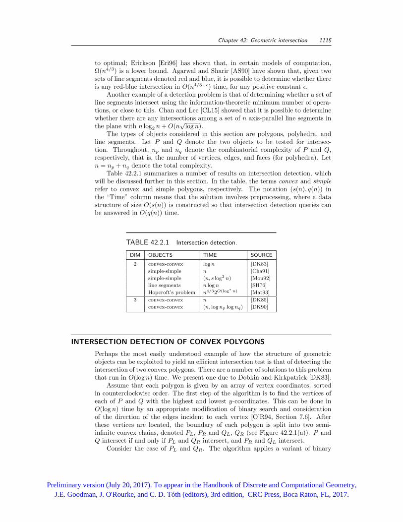
Assume that each polygon is given by an array of vertex coordinates, sortedin counterclockwise order. The first step of the algorithm is to find the vertices ofeach of P and Q with the highest and lowest y-coordinates. This can be done inO(log n) time by an appropriate modification of binary search and considerationof the direction of the edges incident to each vertex [O’R94, Section 7.6]. Afterthese vertices are located, the boundary of each polygon is split into two semi-infinite convex chains, denoted PL, PR and QL, QR (see Figure 42.2.1(a)). P andQ intersect if and only if PL and QR intersect, and PR and QL intersect.

Consider the case of PL and QR. The algorithm applies a variant of binary


1116 David M. Mount

P

PL PR

(a)

QR PL

(b)

QR

PL

(c)

eq

ep

QR

PL

eqep

(d)

FIGURE 42.2.1Intersection detection for two convex polygons.

search. Consider the median edge ep of PL and the median edge eq of QR (shownas heavy lines in the figure). By a simple analysis of the relative positions of theseedges and the intersection point of the two lines on which they lie, it is possibleto determine in constant time either that the polygons intersect, or that half of atleast one of the two boundary chains can be eliminated from further consideration.The cases that arise are illustrated in Figure 42.2.1(b)-(d). The shaded regionsindicate the portion of the boundary that can be eliminated from consideration.

SIMPLE POLYGONS

Without convexity, it is generally not possible to detect intersections in sublineartime without preprocessing; but efficient tests do exist.

One of the important intersection questions is whether a closed polygonal chaindefines the edges of a simple polygon. The problem reduces to detecting whether thechain is self-intersecting. This problem can be solved efficiently by supposing thatthe polygonal chain is a simple polygon, attempting to triangulate the polygon, andseeing whether anything goes wrong in the process. Some triangulation algorithmscan be modified to detect self-intersections. In particular, the problem can be solvedin O(n) time by modifying Chazelle’s linear-time triangulation algorithm [Cha91].See Section 29.2.

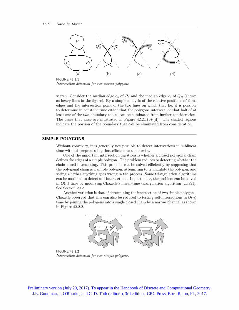
Another variation is that of determining the intersection of two simple polygons.Chazelle observed that this can also be reduced to testing self-intersections in O(n)time by joining the polygons into a single closed chain by a narrow channel as shownin Figure 42.2.2.

FIGURE 42.2.2Intersection detection for two simple polygons.



DETECTING INTERSECTIONS OF MULTIPLE OBJECTS

In many applications, it is important to know whether any pair of a set of objectsintersects one another. Shamos and Hoey showed that the problem of detectingwhether a set of n line segments in the plane have an intersecting pair can besolved in O(n log n) time [SH76]. This is done by plane sweep, which will be dis-cussed below. They also showed that the same can be done for a set of circles.Reichling showed that this can be generalized to detecting whether any pair of mconvex n-gons intersects in O(m logm log n) time, and whether they all share acommon intersection point in O(m log2 n) time [Rei88]. Hopcroft, Schwartz, andSharir [HSS83] showed how to detect the intersection of any pair of n spheres in3-space in O(n log2 n) time and O(n log n) space by applying a 3D plane sweep.

INTERSECTION DETECTION WITH PREPROCESSING

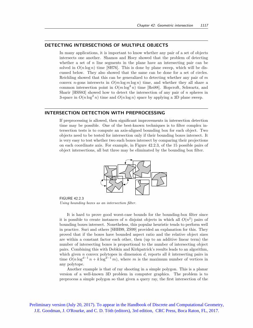
If preprocessing is allowed, then significant improvements in intersection detectiontime may be possible. One of the best-known techniques is to filter complex in-tersection tests is to compute an axis-aligned bounding box for each object. Twoobjects need to be tested for intersection only if their bounding boxes intersect. Itis very easy to test whether two such boxes intersect by comparing their projectionson each coordinate axis. For example, in Figure 42.2.3, of the 15 possible pairs ofobject intersections, all but three may be eliminated by the bounding box filter.

FIGURE 42.2.3Using bounding boxes as an intersection filter.

It is hard to prove good worst-case bounds for the bounding-box filter sinceit is possible to create instances of n disjoint objects in which all O(n2) pairs ofbounding boxes intersect. Nonetheless, this popular heuristic tends to perform wellin practice. Suri and others [SHH99, ZS99] provided an explanation for this. Theyproved that if the boxes have bounded aspect ratio and the relative object sizesare within a constant factor each other, then (up to an additive linear term) thenumber of intersecting boxes is proportional to the number of intersecting objectpairs. Combining this with Dobkin and Kirkpatrick’s results leads to an algorithm,which given n convex polytopes in dimension d, reports all k intersecting pairs intime O(n logd−1 n + k logd−1m), where m is the maximum number of vertices inany polytope.

Another example is that of ray shooting in a simple polygon. This is a planarversion of a well-known 3D problem in computer graphics. The problem is topreprocess a simple polygon so that given a query ray, the first intersection of the


1118 David M. Mount

ray with the boundary of the polygon can be determined. After O(n) preprocessingit is possible to answer ray-shooting queries in O(log n) time. A particularly elegantsolution was given by Hershberger and Suri [HS95]. The polygon is triangulatedin a special way, called a geodesic triangulation, so that any line segment thatdoes not intersect the boundary of the polygon crosses at most O(log n) triangles.Ray-shooting queries are answered by locating the triangle that contains the originof the ray, and “walking” the ray through the triangulation. See also Section 31.2.

Mount showed how the geodesic triangulation can be used to generalize thebounding box test for the intersection of simple polygons. Each polygon is prepro-cessed by computing a geodesic triangulation of its exterior. From this it is possibleto determine whether they intersect in O(s log2 n) time, where s is the minimumnumber of edges in a polygonal chain that separates the two polygons [Mou92].Separation sensitive intersections of polygons has been studied in the context ofkinetic algorithms for collision detection. See Chapter 50.

CONVEX POLYHEDRA IN HIGHER DIMENSIONS

Extending a problem from the plane to 3-space and higher often involves in a signifi-cant increase in difficulty. Computing the intersection of convex polyhedra is amongthe first problems studied in the field of computational geometry [MP78]. Dobkinand Kirkpatrick showed that detecting the intersection of convex polyhedra can beperformed efficiently by adapting Kirkpatrick’s hierarchical decomposition of planartriangulations. Consider convex polyhedra P and Q in 3-space having combinato-rial boundary complexities np and nq, respectively. They showed that each can bepreprocessed in linear time and space so that it is possible to determine the inter-section of any translation and rotation of the two in time O(log np · log nq) [DK90].

DOBKIN-KIRKPATRICK DECOMPOSITION

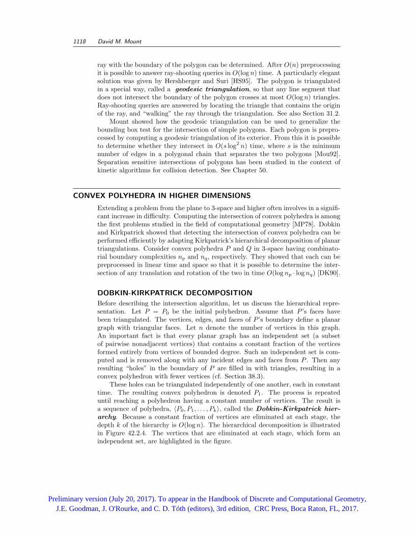
Before describing the intersection algorithm, let us discuss the hierarchical repre-sentation. Let P = P0 be the initial polyhedron. Assume that P ’s faces havebeen triangulated. The vertices, edges, and faces of P ’s boundary define a planargraph with triangular faces. Let n denote the number of vertices in this graph.An important fact is that every planar graph has an independent set (a subsetof pairwise nonadjacent vertices) that contains a constant fraction of the verticesformed entirely from vertices of bounded degree. Such an independent set is com-puted and is removed along with any incident edges and faces from P . Then anyresulting “holes” in the boundary of P are filled in with triangles, resulting in aconvex polyhedron with fewer vertices (cf. Section 38.3).

These holes can be triangulated independently of one another, each in constanttime. The resulting convex polyhedron is denoted P1. The process is repeateduntil reaching a polyhedron having a constant number of vertices. The result isa sequence of polyhedra, 〈P0, P1, . . . , Pk〉, called the Dobkin-Kirkpatrick hier-archy. Because a constant fraction of vertices are eliminated at each stage, thedepth k of the hierarchy is O(log n). The hierarchical decomposition is illustratedin Figure 42.2.4. The vertices that are eliminated at each stage, which form anindependent set, are highlighted in the figure.



FIGURE 42.2.4Dobkin-Kirkpatrick decomposition of a convex polyhedron.

INTERSECTION DETECTION ALGORITHM

Suppose that the hierarchical representations of P and Q have already been com-puted. The intersection detection algorithm actually computes the separation, thatis, the minimum distance between the two polyhedra. First consider the task ofdetermining the separation between P and a triangle T in 3-space. We start withthe top of the hierarchy, Pk. Because Pk and T are both of constant complexity,the separation between Pk and T can be computed in constant time. Given theseparation between Pi and T , it is possible to determine the separation betweenPi−1 and T in constant time. This is done by a consideration of the newly addedboundary elements of Pi−1 that lie in the neighborhood of the two closest points.

Given the hierarchical decompositions of two polyhedra P and Q, the Dobkin-Kirkpatrick intersection algorithm begins by computing the separation at the high-est common level of the two hierarchies (so that at least one of the decomposedpolyhedra is of bounded complexity). They show that in O(log np + log nq) time itis possible to determine the separation of the polyhedra at the next lower level ofthe hierarchies. This leads to a total running time of O(log np · log nq).

IMPROVEMENTS AND HIGHER DIMENSIONS

Barba and Langerman revisited this problem over 30 years after Dobkin and Kirk-patrick’s first result, both improving and extending it. Given convex polyhedraP and Q in d-dimensional space, for any fixed constant d, let np and nq denotetheir respective combinatorial complexities, that is, the total number of faces of alldimensions on their respective boundaries. They show that it is possible to pre-process such polyhedra such that after any translation and rotation, it is possibleto determine whether they intersect in time O(log np + log nq) [BL15]. In 3-space,the preprocessing time and space are linear in the combinatorial complexity. Ingeneral in d-dimensional space the preprocessing time and space are of the form

O(nbd/2c+εp ), for any ε > 0. Their improvement arises by considering intersection

detection from both a primal and polar perspective and applying ε-nets for sam-pling.


1120 David M. Mount

SUBLINEAR INTERSECTION DETECTION

The aforementioned approaches assume that the input polyhedra have been prepro-cessed into a data structure. Without such preprocessing, it would seem impossibleto detect the presence of an intersection in time that is sublinear in the input size.Remarkably, Chazelle, Liu and Magen [CLM05] showed that there exists a random-ized algorithm that, without any preprocessing, detects whether two 3-dimensionaln-vertex convex polyhedra intersect in O(

√n) expected time. Algorithms like this

whose running time is sublinear in the input size are called sublinear algorithms.It is assumed that each polyhedron is presented in memory using any stan-

dard boundary representation, such as a DCEL or winged-edge data structure (seeChapter 67.2.3), and that it is possible to access a random edge or vertex of thepolyhedron in constant time. The algorithm randomly samples O(

√n) vertices from

each polyhedron and applies low-dimensional linear programming to test whetherthe convex hulls of the two sampled sets intersect. If so, the original polyhedra in-tersect. If they do not intersect, the region of possible intersection can be localizedto a portion of the boundary of expected size O(

√n). An efficient algorithm for

identifying and searching this region is presented.

42.3 INTERSECTION COUNTING AND REPORTING

GLOSSARY

Plane sweep: An algorithm paradigm based on simulating the left-to-rightsweep of the plane with a vertical sweepline. See Figure 42.3.1.

Bichromatic intersection: Segment intersection between segments of two col-ors, where only intersections between segments of different colors are to be re-ported (also called red-blue intersection).

In many applications, geometric intersections can be viewed as a discrete set ofentities to be counted or reported. The problems of intersection counting and re-porting have been heavily studied in computational geometry from the perspectiveof intersection searching, employing preprocessing and subsequent queries (Chap-ter 40). We limit our discussion here to batch problems, where the geometricobjects are all given at once. In many instances, the best algorithms known forbatch counting and reporting reduce the problem to intersection searching.

Table 42.3.1 summarizes a number of results on intersection counting and re-porting. The quantity n denotes the combinatorial complexity of the objects, ddenotes the dimension of the space, and k denotes the number of intersections.Because every pair of elements might intersect, the number of intersections k maygenerally be as large as O(n2), but it is frequently much smaller.

Computing the intersection of line segments is among the most fundamentalproblems in computational geometry [Cha86]. It is often an initial step in comput-ing the intersection of more complex objects. In such cases particular properties ofthe class of objects involved may influence the algorithm used for computing theunderlying intersections. For example, if it is known that the objects involved arefat or if only certain faces of the resulting arrangement are of interest, then moreefficient approaches may be possible (see, e.g., [AMS98, MPS+94, Vig03]).



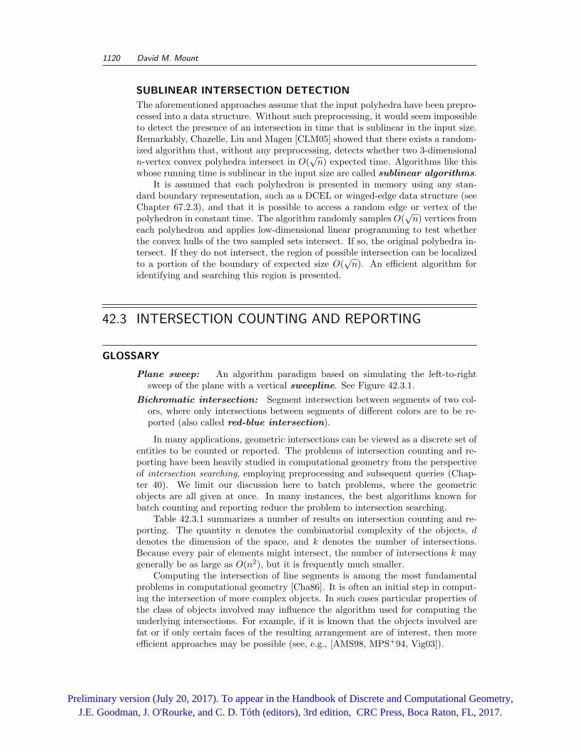
TABLE 42.3.1 Intersection counting and reporting.

PROBLEM DIM OBJECTS TIME SOURCE

Reporting 2 line segments n logn+ k [CE92][Bal95]

2 bichromatic segments (general) n4/3 logO(1) n+ k [Aga90][Cha93]

2 bichromatic segments (disjoint) n+ k [FH95]

d orthogonal segments n logd−1 n+ k [EM81]

Counting 2 line segments n4/3 logO(1) n [Aga90][Cha93]

2 bichromatic segments (general) n4/3 logO(1) n [Aga90][Cha93]

2 bichromatic segments (disjoint) n logn [CEGS94]

d orthogonal segments n logd−1 n [EM81, Cha88]

A related problem is that of computing properties of the set of intersectionpoints of a collection of objects. Atallah showed that it is possible to compute theconvex hull of the (quadratic sized) set of intersection points of a collection of nlines in the plane in time O(n log n) [?]. Arkin et al. [AMS08] showed that it ispossible to achieve the same running time for the more general case of intersectionpoints of line segments in the plane.

REPORTING LINE SEGMENT INTERSECTIONS

Consider the problem of reporting the intersections of n line segments in the plane.This problem is an excellent vehicle for introducing the powerful technique of planesweep (Figure 42.3.1). The plane-sweep algorithm maintains an active list of seg-ments that intersect the current sweepline, sorted from bottom to top by inter-section point. If two line segments intersect, then at some point prior to thisintersection they must be consecutive in the sweep list. Thus, we need only testconsecutive pairs in this list for intersection, rather than testing all O(n2) pairs.

At each step the algorithm advances the sweepline to the next event: a linesegment endpoint or an intersection point between two segments. Events are storedin a priority queue by their x-coordinates. After advancing the sweepline to thenext event point, the algorithm updates the contents of the active list, tests newconsecutive pairs for intersection, and inserts any newly-discovered events in thepriority queue. For example, in Figure 42.3.1 the locations of the sweepline areshown with dashed lines.

FIGURE 42.3.1Plane sweep for line segment intersection.


1122 David M. Mount

Bentley and Ottmann [BO79] showed that by using plane sweep it is possibleto report all k intersecting pairs of n line segments in O((n+ k) log n) time. If thenumber of intersections k is much less than the O(n2) worst-case bound, then thisis great savings over a brute-force test of all pairs.

For many years the question of whether this could be improved to O(n log n+k)was open, until Edelsbrunner and Chazelle presented such an algorithm [CE92].This algorithm is optimal with respect to running time because at least Ω(k) timeis needed to report the result, and it can be shown that Ω(n log n) time is neededto detect whether there is any intersection at all. However, their algorithm usesO(n + k) space. Balaban [Bal95] showed how to achieve the same running timeusing only O(n) space. Vahrenhold [Vah07] further improved the space bound byshowing that there is an in-place algorithm that runs in time O(n log2 n + k).This means that the input is assumed to be stored in an array of size n so thatrandom access is possible and only O(1) additional working space is needed.

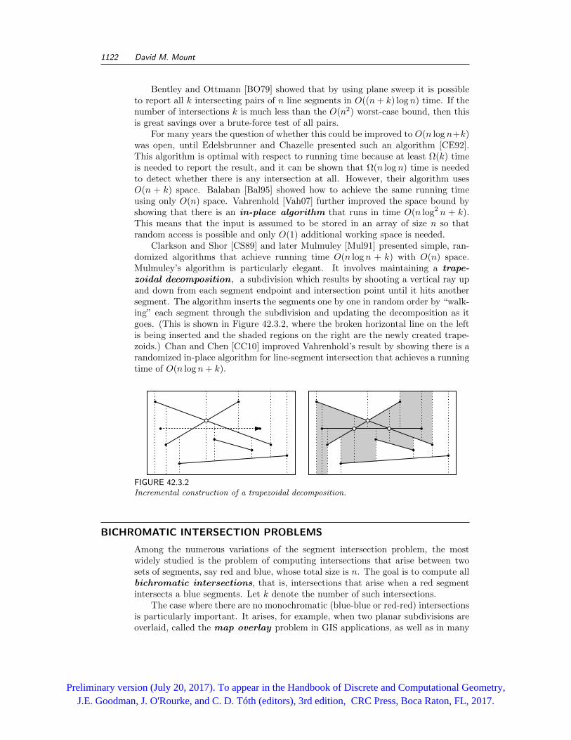
Clarkson and Shor [CS89] and later Mulmuley [Mul91] presented simple, ran-domized algorithms that achieve running time O(n log n + k) with O(n) space.Mulmuley’s algorithm is particularly elegant. It involves maintaining a trape-zoidal decomposition , a subdivision which results by shooting a vertical ray upand down from each segment endpoint and intersection point until it hits anothersegment. The algorithm inserts the segments one by one in random order by “walk-ing” each segment through the subdivision and updating the decomposition as itgoes. (This is shown in Figure 42.3.2, where the broken horizontal line on the leftis being inserted and the shaded regions on the right are the newly created trape-zoids.) Chan and Chen [CC10] improved Vahrenhold’s result by showing there is arandomized in-place algorithm for line-segment intersection that achieves a runningtime of O(n log n+ k).

FIGURE 42.3.2Incremental construction of a trapezoidal decomposition.

BICHROMATIC INTERSECTION PROBLEMS

Among the numerous variations of the segment intersection problem, the mostwidely studied is the problem of computing intersections that arise between twosets of segments, say red and blue, whose total size is n. The goal is to compute allbichromatic intersections, that is, intersections that arise when a red segmentintersects a blue segments. Let k denote the number of such intersections.

The case where there are no monochromatic (blue-blue or red-red) intersectionsis particularly important. It arises, for example, when two planar subdivisions areoverlaid, called the map overlay problem in GIS applications, as well as in many



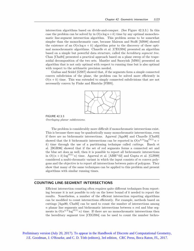
intersection algorithms based on divide-and-conquer. (See Figure 42.3.3.) In thiscase the problem can be solved by in O(n log n+k) time by any optimal monochro-matic line-segment intersection algorithm. This problem seems to be somewhatsimpler than the monochromatic case, because Mairson and Stolfi [MS88] showedthe existence of an O(n log n + k) algorithm prior to the discovery of these opti-mal monochromatic algorithms. Chazelle et al. [CEGS94] presented an algorithmbased on a simple but powerful data structure, called the hereditary segment tree.Chan [Cha94] presented a practical approach based on a plane sweep of the trape-zoidal decomposition of the two sets. Mantler and Snoeyink [MS01] presented analgorithm that is not only optimal with respect to running time but is also optimalwith respect to the arithmetic precision needed.

Guibas and Seidel [GS87] showed that, if the segments form a simple connectedconvex subdivision of the plane, the problem can be solved more efficiently inO(n + k) time. This was extended to simply connected subdivisions that are notnecessarily convex by Finke and Hinrichs [FH95].

FIGURE 42.3.3Overlaying planar subdivisions.

The problem is considerably more difficult if monochromatic intersections exist.This is because there may be quadratically many monochromatic intersections, evenif there are no bichromatic intersections. Agarwal [Aga90] and Chazelle [Cha93]

showed that the k bichromatic intersections can be reported in O(n4/3 logO(1) n +k) time through the use of a partitioning technique called cuttings. Basch etal. [BGR96] showed that if the set of red segments forms a connected set andthe blue set does as well, then it is possible to report all bichromatic intersectionsin O((n + k) logO(1) n) time. Agarwal et al. [ABH+02] and Gupta et al. [GJS99]considered a multi-chromatic variant in which the input consists of m convex poly-gons and the objective is to report all intersections between pairs of polygons. Theyshow that many of the same techniques can be applied to this problem and presentalgorithms with similar running times.

COUNTING LINE-SEGMENT INTERSECTIONS

Efficient intersection counting often requires quite different techniques from report-ing because it is not possible to rely on the lower bound of k needed to report theresults. Nonetheless, a number of the efficient intersection reporting algorithmscan be modified to count intersections efficiently. For example, methods based oncuttings [Aga90, Cha93] can be used to count the number of intersections amongn planar line segments and bichromatic intersections between n red and blue seg-ments in O(n4/3 logO(1) n) time. If there are no monochromatic intersections thenthe hereditary segment tree [CEGS94] can be used to count the number bichro-


1124 David M. Mount

matic intersections in O(n log n) time. Chan and Wilkinson showed that in theword RAM computational model it is possible to count bichromatic intersectionseven faster in O(n

√log n) time [CW11].

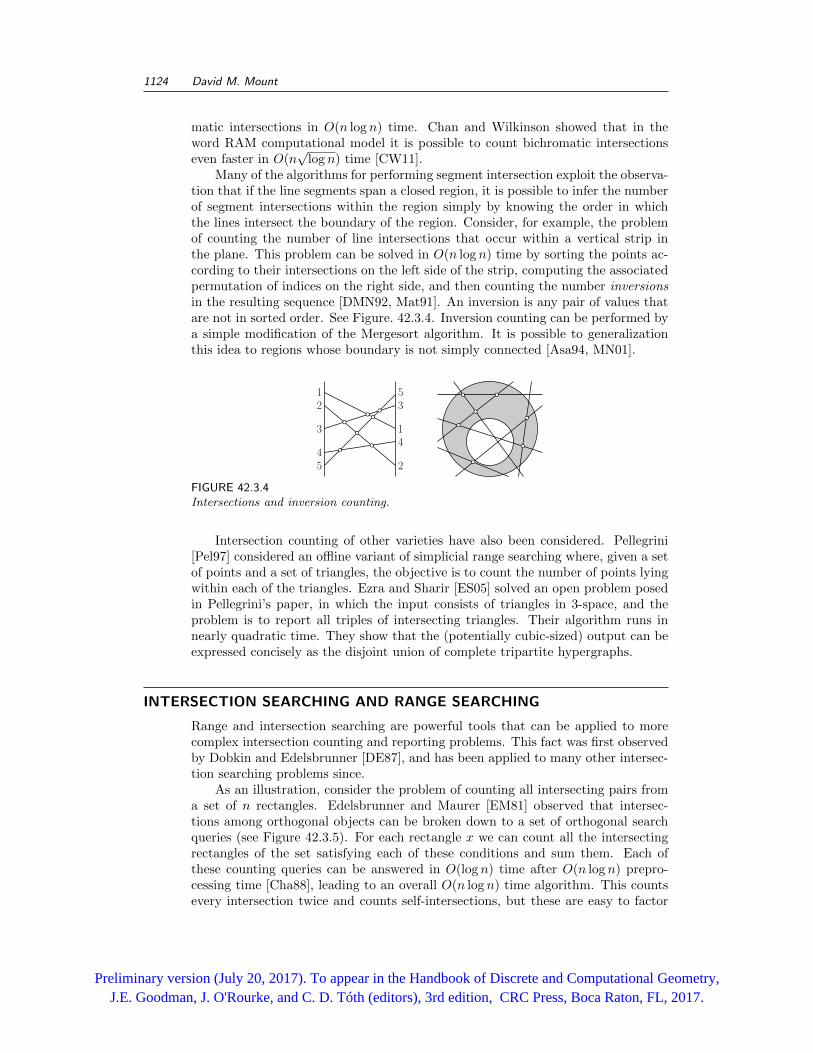
Many of the algorithms for performing segment intersection exploit the observa-tion that if the line segments span a closed region, it is possible to infer the numberof segment intersections within the region simply by knowing the order in whichthe lines intersect the boundary of the region. Consider, for example, the problemof counting the number of line intersections that occur within a vertical strip inthe plane. This problem can be solved in O(n log n) time by sorting the points ac-cording to their intersections on the left side of the strip, computing the associatedpermutation of indices on the right side, and then counting the number inversionsin the resulting sequence [DMN92, Mat91]. An inversion is any pair of values thatare not in sorted order. See Figure. 42.3.4. Inversion counting can be performed bya simple modification of the Mergesort algorithm. It is possible to generalizationthis idea to regions whose boundary is not simply connected [Asa94, MN01].

12

3

45

1

2

3

4

5

FIGURE 42.3.4Intersections and inversion counting.

Intersection counting of other varieties have also been considered. Pellegrini[Pel97] considered an offline variant of simplicial range searching where, given a setof points and a set of triangles, the objective is to count the number of points lyingwithin each of the triangles. Ezra and Sharir [ES05] solved an open problem posedin Pellegrini’s paper, in which the input consists of triangles in 3-space, and theproblem is to report all triples of intersecting triangles. Their algorithm runs innearly quadratic time. They show that the (potentially cubic-sized) output can beexpressed concisely as the disjoint union of complete tripartite hypergraphs.

INTERSECTION SEARCHING AND RANGE SEARCHING

Range and intersection searching are powerful tools that can be applied to morecomplex intersection counting and reporting problems. This fact was first observedby Dobkin and Edelsbrunner [DE87], and has been applied to many other intersec-tion searching problems since.

As an illustration, consider the problem of counting all intersecting pairs froma set of n rectangles. Edelsbrunner and Maurer [EM81] observed that intersec-tions among orthogonal objects can be broken down to a set of orthogonal searchqueries (see Figure 42.3.5). For each rectangle x we can count all the intersectingrectangles of the set satisfying each of these conditions and sum them. Each ofthese counting queries can be answered in O(log n) time after O(n log n) prepro-cessing time [Cha88], leading to an overall O(n log n) time algorithm. This countsevery intersection twice and counts self-intersections, but these are easy to factor



out from the final result. Generalizations to hyperrectangle intersection countingin higher dimensions are straightforward, with an additional factor of log n in timeand space for each increase in dimension. We refer the reader to Chapter 40 formore information on intersection searching and its relationship to range searching.

x

y

xx

yy

y

x

FIGURE 42.3.5Types of intersections between rectangles x and y.

42.4 INTERSECTION CONSTRUCTION

GLOSSARY

Regularization: Discarding measure-zero parts of the result of an operation bytaking the closure of the interior.

Clipping: Computing the intersection of each of many polygons with an axis-aligned rectangular viewing window.

Kernel of a polygon: The set of points that can see every point of the polygon.(See Section 30.1.)

Intersection construction involves determining the region of intersection be-tween geometric objects. Many of the same techniques that are used for computinggeometric intersections are used for computing Boolean operations in general (e.g.,union and difference). Many of the results presented here can be applied to theseother problems as well. Typically intersection construction reduces to the followingtasks: (1) compute the intersection between the boundaries of the objects; (2) if theboundaries do not intersect then determine whether one object is nested within theother; and (3) if the boundaries do intersect then classify the resulting boundaryfragments and piece together the final intersection region.

(a) (b) (c)

QP

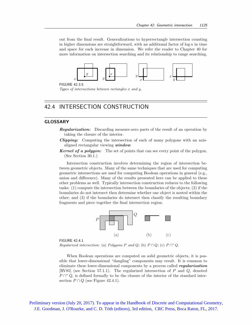
FIGURE 42.4.1Regularized intersection: (a) Polygons P and Q; (b) P ∩Q; (c) P ∩∗ Q.

When Boolean operations are computed on solid geometric objects, it is pos-sible that lower-dimensional “dangling” components may result. It is common toeliminate these lower-dimensional components by a process called regularization[RV85] (see Section 57.1.1). The regularized intersection of P and Q, denotedP ∩∗ Q, is defined formally to be the closure of the interior of the standard inter-section P ∩Q (see Figure 42.4.1).


1126 David M. Mount

Some results on intersection construction are summarized in Table 42.4.1, wheren is the total complexity of the objects being intersected, and k is the number ofpairs of intersecting edges.

TABLE 42.4.1 Intersection construction.

DIM OBJECTS TIME SOURCE

2 convex-convex n [SH76, OCON82]

2 simple-simple n logn+ k [CE92]

2 kernel n [LP79]

3 convex-convex n [Cha92]

CONVEX POLYGONS

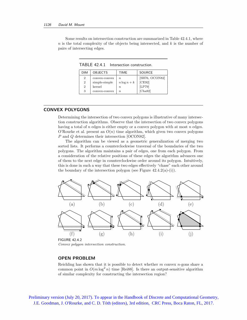
Determining the intersection of two convex polygons is illustrative of many intersec-tion construction algorithms. Observe that the intersection of two convex polygonshaving a total of n edges is either empty or a convex polygon with at most n edges.O’Rourke et al. present an O(n) time algorithm, which given two convex polygonsP and Q determines their intersection [OCON82].

The algorithm can be viewed as a geometric generalization of merging twosorted lists. It performs a counterclockwise traversal of the boundaries of the twopolygons. The algorithm maintains a pair of edges, one from each polygon. Froma consideration of the relative positions of these edges the algorithm advances oneof them to the next edge in counterclockwise order around its polygon. Intuitively,this is done in such a way that these two edges effectively “chase” each other aroundthe boundary of the intersection polygon (see Figure 42.4.2(a)-(i)).

(a) (b) (c) (d) (e)

(f) (g) (h) (i) (j)FIGURE 42.4.2Convex polygon intersection construction.

OPEN PROBLEM

Reichling has shown that it is possible to detect whether m convex n-gons share acommon point in O(m log2 n) time [Rei88]. Is there an output-sensitive algorithmof similar complexity for constructing the intersection region?



SIMPLE POLYGONS AND CLIPPING

As with convex polygons, computing the intersection of two simple polygons re-duces to first computing the points at which the two boundaries intersect and thenclassifying the resulting edge fragments. Computing the edge intersections and edgefragments can be performed by any algorithm for reporting line segment intersec-tions. Classifying the edge fragments is a simple task. Margalit and Knott describea method for edge classification that works not only for intersection, but for anyBoolean operation on the polygons [MK89].

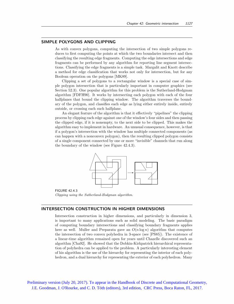
Clipping a set of polygons to a rectangular window is a special case of sim-ple polygon intersection that is particularly important in computer graphics (seeSection 52.3). One popular algorithm for this problem is the Sutherland-Hodgmanalgorithm [FDFH90]. It works by intersecting each polygon with each of the fourhalfplanes that bound the clipping window. The algorithm traverses the bound-ary of the polygon, and classifies each edge as lying either entirely inside, entirelyoutside, or crossing each such halfplane.

An elegant feature of the algorithm is that it effectively “pipelines” the clippingprocess by clipping each edge against one of the window’s four sides and then passingthe clipped edge, if it is nonempty, to the next side to be clipped. This makes thealgorithm easy to implement in hardware. An unusual consequence, however, is thatif a polygon’s intersection with the window has multiple connected components (ascan happen with a nonconvex polygon), then the resulting clipped polygon consistsof a single component connected by one or more “invisible” channels that run alongthe boundary of the window (see Figure 42.4.3).

FIGURE 42.4.3Clipping using the Sutherland-Hodgman algorithm.

INTERSECTION CONSTRUCTION IN HIGHER DIMENSIONS

Intersection construction in higher dimensions, and particularly in dimension 3,is important to many applications such as solid modeling. The basic paradigmof computing boundary intersections and classifying boundary fragments applieshere as well. Muller and Preparata gave an O(n log n) algorithm that computesthe intersection of two convex polyhedra in 3-space (see [PS85]). The existence ofa linear-time algorithm remained open for years until Chazelle discovered such analgorithm [Cha92]. He showed that the Dobkin-Kirkpatrick hierarchical representa-tion of polyhedra can be applied to the problem. A particularly interesting elementof his algorithm is the use of the hierarchy for representing the interior of each poly-hedron, and a dual hierarchy for representing the exterior of each polyhedron. Many


1128 David M. Mount

years later Chan presented a significantly simpler algorithm, which also uses theDobkin-Kirkpatrick hierarchy [Cha16]. Dobrindt, Mehlhorn, and Yvinec [DMY93]presented an output-sensitive algorithm for intersecting two polyhedra, one of whichis convex.

Another class of problems can be solved efficiently are those involving polyhedralterrains, that is, a polyhedral surface that intersects every vertical line in at mostone point. Chazelle et al. [CEGS94] show that the hereditary segment tree can beapplied to compute the smallest vertical distance between two polyhedral terrains inroughly O(n4/3) time. They also show that the upper envelope of two polyhedralterrains can be computed in O(n3/2+ε + k log2 n) time, where ε is an arbitraryconstant and k is the number of edges in the upper envelope.

KERNELS AND THE INTERSECTION OF HALFSPACES

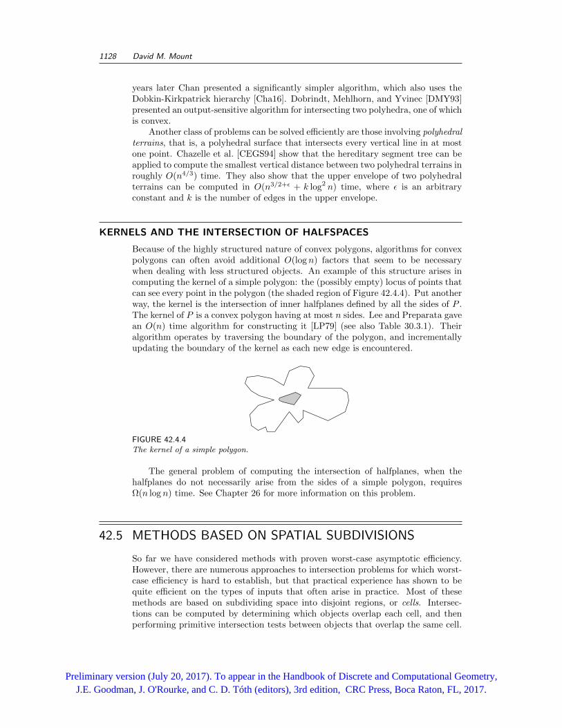
Because of the highly structured nature of convex polygons, algorithms for convexpolygons can often avoid additional O(log n) factors that seem to be necessarywhen dealing with less structured objects. An example of this structure arises incomputing the kernel of a simple polygon: the (possibly empty) locus of points thatcan see every point in the polygon (the shaded region of Figure 42.4.4). Put anotherway, the kernel is the intersection of inner halfplanes defined by all the sides of P .The kernel of P is a convex polygon having at most n sides. Lee and Preparata gavean O(n) time algorithm for constructing it [LP79] (see also Table 30.3.1). Theiralgorithm operates by traversing the boundary of the polygon, and incrementallyupdating the boundary of the kernel as each new edge is encountered.

FIGURE 42.4.4The kernel of a simple polygon.

The general problem of computing the intersection of halfplanes, when thehalfplanes do not necessarily arise from the sides of a simple polygon, requiresΩ(n log n) time. See Chapter 26 for more information on this problem.

42.5 METHODS BASED ON SPATIAL SUBDIVISIONS

So far we have considered methods with proven worst-case asymptotic efficiency.However, there are numerous approaches to intersection problems for which worst-case efficiency is hard to establish, but that practical experience has shown to bequite efficient on the types of inputs that often arise in practice. Most of thesemethods are based on subdividing space into disjoint regions, or cells. Intersec-tions can be computed by determining which objects overlap each cell, and thenperforming primitive intersection tests between objects that overlap the same cell.



GRIDS

Perhaps the simplest spatial subdivision is based on “bucketing” with square grids.Space is subdivided into a regular grid of squares (or generally hypercubes) ofequal side length. The side length is typically chosen so that either the totalnumber of cells is bounded, or the expected number of objects overlapping eachcell is bounded. Edahiro et al. [ETHA89] showed that this method is competitivewith and often performs much better than more sophisticated data structures forreporting intersections between randomly generated line segments in the plane.Conventional wisdom is that grids perform well as long as the objects are small onaverage and their distribution is roughly uniform.

HIERARCHICAL SUBDIVISIONS

The principle shortcoming of grids is their inability to deal with nonuniformlydistributed objects. Hierarchical subdivisions of space are designed to overcome thisweakness. There is quite a variety of different data structures based on hierarchicalsubdivisions, but almost all are based on the principal of recursively subdividingspace into successively smaller regions, until each region is sufficiently simple in thesense that it overlaps only a small number of objects. When a region is subdivided,the resulting subregions are its children in the hierarchy. Well-known examplesof hierarchical subdivisions for storing geometric objects include quadtrees and k-dtrees, R-trees, and binary space partition (BSP) trees. See [Sam90b] for a discussionof all of these.

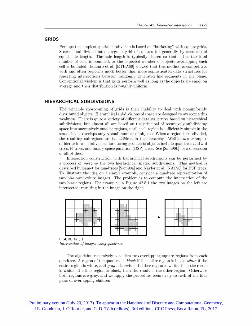
Intersection construction with hierarchical subdivisions can be performed bya process of merging the two hierarchical spatial subdivisions. This method isdescribed by Samet for quadtrees [Sam90a] and Naylor et al. [NAT90] for BSP trees.To illustrate the idea on a simple example, consider a quadtree representation oftwo black-and-white images. The problem is to compute the intersection of thetwo black regions. For example, in Figure 42.5.1 the two images on the left areintersected, resulting in the image on the right.

FIGURE 42.5.1Intersection of images using quadtrees.

The algorithm recursively considers two overlapping square regions from eachquadtree. A region of the quadtree is black if the entire region is black, white if theentire region is white, and gray otherwise. If either region is white, then the resultis white. If either region is black, then the result is the other region. Otherwiseboth regions are gray, and we apply the procedure recursively to each of the fourpairs of overlapping children.


1130 David M. Mount

42.6 SOURCES

Geometric intersections and related topics are covered in general sources on compu-tational geometry [BCKO00, O’R94, Mul93, Ede87, PS85, Meh84]. A good sourceof information on the complexity of the lower envelopes and faces in arrangementsare the books by Agarwal [Aga91] and Sharir and Agarwal [SA95]. Intersectionsof convex objects are discussed in the paper by Chazelle and Dobkin [CD87].For information on data structures useful for geometric intersections see Samet’sbooks [Sam90a, Sam90b, Sam06]. Sources on computing intersection primitives in-clude O’Rourke’s book on computational geometry [O’R94], Yap’s book [Yap93] onalgebraic algorithms, and most texts on computer graphics, for example [FDFH90].For 3D surface intersections, consult books on solid modeling, including those byHoffmann [Hof89] and Mantyla [Man88]. The Graphics Gems series (e.g., [Pae95])contains a number of excellent tips and techniques for computing geometric oper-ations including intersection primitives.

RELATED CHAPTERS

Chapter 26: Convex hull computationsChapter 28: ArrangementsChapter 29: Triangulations and mesh generationChapter 40: Range searchingChapter 41: Ray shooting and lines in spaceChapter 52: Computer graphicsChapter 56: Splines and geometric modeling

REFERENCES

[ABD+97] F. Avnaim, J.-D. Boissonnat, O. Devillers, F.P. Preparata, and M. Yvinec. Evaluating

signs of determinants using single-precision arithmetic. Algorithmica, 17:111–132, 1997.

[ABH+02] P.K. Agarwal, M. de Berg, S. Har-Peled, M.H. Overmars, M. Sharir, and J. Vahrenhold.

Reporting intersecting pairs of convex polytopes in two and three dimensions. Comput.

Geom., 23:197–207, 2002.

[Aga90] P.K. Agarwal. Partitioning arrangements of lines: II. Applications. Discrete Comput.

Geom., 5:533–573, 1990.

[Aga91] P.K. Agarwal. Intersection and Decomposition Algorithms for Planar Arrangements.

Cambridge University Press, New York, 1991.

[AKO93] P.K. Agarwal, M. van Kreveld, and M. Overmars. Intersection queries in curved

objects. J. Algorithms, 15:229–266, 1993.

[AMS98] P.K. Agarwal, J. Matousek, and O. Schwarzkopf. Computing many faces in arrange-

ments of lines and segments. SIAM J. Comput., 27:491–505, 1998.

[AMS08] E.M. Arkin, J.S.B. Mitchell, and J. Snoeyink. Capturing crossings: Convex hulls of

segment and plane intersections. Inform. Process. Lett., 107:194–197, 2008.

[APS93] P.K. Agarwal, M. Pellegrini, and M. Sharir. Counting circular arc intersections. SIAM

J. Comput., 22:778–793, 1993.



[AS90] P.K. Agarwal and M. Sharir. Red-blue intersection detection algorithms, with appli-

cations to motion planning and collision detection. SIAM J. Comput., 19:297–321,

1990.

[Asa94] T. Asano. Reporting and counting intersections of lines within a polygon. In Proc. 5th

Internat. Sympos. Algorithms Comput., vol. 834 of LNCS, pages 652–659, Springer,

Berlin, 1994.

[Bal95] I.J. Balaban. An optimal algorithm for finding segment intersections. In Proc. 11th

Sympos. Comput. Geom., pages 211–219, ACM Press, 1995.

[BCKO00] M. de Berg, O. Cheong, M. van Kreveld, and M. Overmars. Computational Geometry:

Algorithms and Applications. Springer-Verlag, Berlin, 3rd edition, 2008.

[BGR96] J. Basch, L.J. Guibas, and G.D. Ramkumar. Reporting red-blue intersections be-

tween two sets of connected line segments. In Proc. 4th European Sympos. Algorithms,

vol. 1136 of LNCS, pages 302–319, Springer, Berlin, 1996.

[BHO07] M. de Berg, D. Halperin, and M. Overmars. An intersection-sensitive algorithm for

snap rounding. Comput. Geom., 36:159–165, 2007.

[BKM+95] C. Burnikel, J. Konnemann, K. Mehlhorn, S. Naher, S. Schirra, and C. Uhrig. Exact

geometric computation in LEDA. In Proc. 11th Sympos. Comput. Geom., pages C18–

C19, 1995.

[BL15] L. Barba and S. Langerman. Optimal detection of intersections between convex poly-

hedra. In Proc. 26th ACM-SIAM Sympos. Discrete Algorithms, pages 1641–1654, 2015.

[BO79] J.L. Bentley and T.A. Ottmann. Algorithms for reporting and counting geometric

intersections. IEEE Trans. Comput., C-28:643–647, 1979.

[BS00] J.-D. Boissonnat and J. Snoeyink. Efficient algorithms for line and curve segment

intersection using restricted predicates. Comput. Geom, 16:35–52, 2000.

[BV02] J.-D. Boissonnat and A. Vigneron. An elementary algorithm for reporting intersections

of red/blue curve segments. Comput. Geom., 21:167–175, 2002.

[CC10] T.M. Chan and E.Y. Chen. Optimal in-place and cache-oblivious algorithms for 3-d

convex hulls and 2-d segment intersection. Comput. Geom., 43:636–646, 2010.

[CD87] B. Chazelle and D.P. Dobkin. Intersection of convex objects in two and three dimen-

sions. J. ACM, 34:1–27, 1987.

[CE92] B. Chazelle and H. Edelsbrunner. An optimal algorithm for intersecting line segments

in the plane. J. ACM, 39:1–54, 1992.

[CEGS91] B. Chazelle, H. Edelsbrunner, L.J. Guibas, and M. Sharir. A singly exponential strati-

fication scheme for real semi-algebraic varieties and its applications. Theoret. Comput.

Sci., 84:77–105, 1991.

[CEGS94] B. Chazelle, H. Edelsbrunner, L.J. Guibas, and M. Sharir. Algorithms for bichromatic

line segment problems and polyhedral terrains. Algorithmica, 11:116–132, 1994.

[Cha86] B. Chazelle. Reporting and counting segment intersections. J. Comput. Syst. Sci.,

32:156–182, 1986.

[Cha88] B. Chazelle. A functional approach to data structures and its use in multidimensional

searching. SIAM J. Comput., 17:427–462, 1988.

[Cha91] B. Chazelle. Triangulating a simple polygon in linear time. Discrete Comput. Geom.,

6:485–524, 1991.

[Cha92] B. Chazelle. An optimal algorithm for intersecting three-dimensional convex polyhedra.

SIAM J. Comput., 21:671–696, 1992.


1132 David M. Mount

[Cha93] B. Chazelle. Cutting hyperplanes for divide-and-conquer. Discrete Comput. Geom.,

9:145–158, 1993.

[Cha94] T.M. Chan. A simple trapezoid sweep algorithm for reporting red/blue segment inter-

sections. In Proc. 6th Canad. Conf. Comput. Geom., pages 263–268, 1994.

[Cha16] T.M. Chan. A simpler linear-time algorithm for intersecting two convex polyhedra in

three dimensions. Discrete Comput. Geom., 56:860–865, 2016.

[CL15] T.M. Chan and P. Lee. On constant factors in comparison-based geometric algorithms

and data structures. Discrete Comput. Geom., 53:489–513, 2015.

[Cla92] K.L. Clarkson. Safe and effective determinant evaluation. In Proc. 33rd IEEE Sympos.

Found. Comput. Sci., pages 387–395, 1992.

[CLM05] B. Chazelle, D. Liu, and A. Magen. Sublinear geometric algorithms. SIAM J. Comput.,

35:627–646, 2005.

[CS89] K.L. Clarkson and P.W. Shor. Applications of random sampling in computational

geometry, II. Discrete Comput. Geom., 4:387–421, 1989.

[CW11] T.M. Chan and B.T. Wilkinson. Bichromatic line segment intersection counting in

o(n√

logn) time. In Proc. 23rd Canadian Conf. Comput. Geom., Toronto, 2011.

[DE87] D.P. Dobkin and H. Edelsbrunner. Space searching for intersecting objects. J. Algo-

rithms, 8:348–361, 1987.

[DK83] D.P. Dobkin and D.G. Kirkpatrick. Fast detection of polyhedral intersection. Theoret.

Comput. Sci., 27:241–253, 1983.

[DK85] D.P. Dobkin and D.G. Kirkpatrick. A linear algorithm for determining the separation

of convex polyhedra. J. Algorithms, 6:381–392, 1985.

[DK90] D.P. Dobkin and D.G. Kirkpatrick. Determining the separation of preprocessed

polyhedra—a unified approach. In Proc. 17th Internat. Colloq. Automata Lang. Pro-

gram., vol. 443 of LNCS, pages 400–413, Springer, Berlin, 1990.

[DMN92] M.B. Dillencourt, D.M. Mount, and N.S. Netanyahu. A randomized algorithm for

slope selection. Internat. J. Comput. Geom. Appl., 2:1–27, 1992.

[DMY93] K. Dobrindt, K. Mehlhorn, and M. Yvinec. A complete and efficient algorithm for the

intersection of a general and a convex polyhedron. In Proc. 3rd Workshop Algorithms

Data Struct., vol. 709 of LNCS, pages 314–324, Springer, Berlin, 1993.

[Ede87] H. Edelsbrunner. Algorithms in Combinatorial Geometry, vol. 10 of EATCS Monogr.

Theoret. Comput. Sci. Springer-Verlag, Heidelberg, 1987.

[EM81] H. Edelsbrunner and H.A. Maurer. On the intersection of orthogonal objects. Inform.

Process. Lett., 13:177–181, 1981.

[Eri96] J. Erickson. New lower bounds for Hopcroft’s problem. Discrete Comput. Geom.,

16:389–418, 1996.

[ES05] E. Ezra and M. Sharir. Counting and representing intersections among triangles in

three dimensions. Comput. Geom., 32:196–215, 2005.

[ETHA89] M. Edahiro, K. Tanaka, R. Hoshino, and Ta. Asano. A bucketing algorithm for the or-

thogonal segment intersection search problem and its practical efficiency. Algorithmica,

4:61–76, 1989.

[FDFH90] J.D. Foley, A. van Dam, S.K. Feiner, and J.F. Hughes. Computer Graphics: Principles

and Practice. Addison-Wesley, Reading, 1990.

[FH95] U. Finke and K.H. Hinrichs. Overlaying simply connected planar subdivisions in linear

time. In Proc. 11th Sympos. Comput. Geom., pages 119–126, ACM Press, 1995.



[FW96] S. Fortune and C.J. van Wyk. Static analysis yields efficient exact integer arithmetic

for computational geometry. ACM Trans. Graph., 15:223–248, 1996.

[GJS99] P. Gupta, R. Janardan, and M. Smid. Efficient algorithms for counting and reporting

pairwise intersections between convex polygons. Inform. Process. Lett., 69:7–13, 1999.

[GS87] L.J. Guibas and R. Seidel. Computing convolutions by reciprocal search. Discrete

Comput. Geom., 2:175–193, 1987.

[GY86] D.H. Greene and F.F. Yao. Finite-resolution computational geometry. In Proc. 27th

IEEE Sympos. Found. Comp. Sci., pages 143–152, 1986.

[Her13] J. Hershberger. Stable snap rounding. Comput. Geom., 46:403–416, 2013.

[Hob99] J.D. Hobby. Practical segment intersection with finite precision output. Comput.

Geom., 13:199–214, 1999.

[Hof89] C.M. Hoffmann. Geometric and Solid Modeling. Morgan Kaufmann, San Francisco,

1989.

[HP02] D. Halperin and E. Packer. Iterated snap rounding. Comput. Geom., 23:209–225, 2002.

[HS95] J. Hershberger and S. Suri. A pedestrian approach to ray shooting: Shoot a ray, take

a walk. J. Algorithms, 18:403–431, 1995.

[HSS83] J.E. Hopcroft, J.T. Schwartz, and M. Sharir. Efficient detection of intersections among

spheres. Internat. J. Robot. Res., 2:77–80, 1983.

[JG91] J.K. Johnstone and M.T. Goodrich. A localized method for intersecting plane algebraic

curve segments. Visual Comput., 7:60–71, 1991.

[LP79] D.T. Lee and F.P. Preparata. An optimal algorithm for finding the kernel of a polygon.

J. ACM, 26:415–421, 1979.

[LP79b] J.J. Little and T.K. Peucker. A recursive procedure for finding the intersection of two

digital curves. Comput. Graph. Image Process., 10:159–171, 1979.

[Man88] M. Mantyla. An Introduction to Solid Modeling. Computer Science Press, Rockville,

1988.

[Mat91] J. Matousek. Randomized optimal algorithm for slope selection. Inform. Process. Lett.,

39:183–187, 1991.

[Mat93] J. Matousek. Range searching with efficient hierarchical cuttings. Discrete Comput.

Geom., 10:157–182, 1993.

[MC91] D. Manocha and J.F. Canny. A new approach for surface intersection. Internat. J.

Comput. Geom. Appl., 1:491–516, 1991.

[Meh84] K. Mehlhorn. Multi-dimensional Searching and Computational Geometry, vol. 3 of

Data Structures and Algorithms, Springer-Verlag, Berlin, 1984.

[MK89] A. Margalit and G.D. Knott. An algorithm for computing the union, intersection or

difference of two polygons. Comput. Graph., 13:167–183, 1989.

[MN01] D.M. Mount and N.S. Netanyahu. Efficient randomized algorithms for robust estima-

tion of circular arcs and aligned ellipses. Comput. Geom., 19:1–33, 2001.

[Mou92] D.M. Mount. Intersection detection and separators for simple polygons. In Proc. 8th

Sympos. Comput. Geom., pages 303–311, ACM Press, 1992.

[MP78] D.E. Muller and F.P. Preparata. Finding the intersection of two convex polyhedra.

Theoret. Comput. Sci., 7:217–236, 1978.

[MPS+94] J. Matousek, J. Pach, M. Sharir, S. Sifrony, and E. Welzl. Fat triangles determine

linearly many holes. SIAM J. Comput., 23:154–169, 1994.


1134 David M. Mount

[MS88] H.G. Mairson and J. Stolfi. Reporting and counting intersections between two sets

of line segments. In R.A. Earnshaw, editor, Theoretical Foundations of Computer

Graphics and CAD, vol. F40 of NATO ASI, pages 307–325, Springer, Berlin, 1988.

[MS01] A. Mantler and J. Snoeyink. Intersecting red and blue line segments in optimal time

and precision. In Japan. Conf. Discrete Comput. Geom., vol. 2098 of LNCS, pages

244–251, Springer, Berlin, 2001.

[Mul91] K. Mulmuley. A fast planar partition algorithm, II. J. ACM, 38:74–103, 1991.

[Mul93] K. Mulmuley. Computational Geometry: An Introduction through Randomized Algo-

rithms. Prentice Hall, Englewood Cliffs, 1993.

[NAT90] B. Naylor, J.A. Amatodes, and W. Thibault. Merging BSP trees yields polyhedral set

operations. Comput. Graph., 24:115–124, 1990.

[OCON82] J. O’Rourke, C.-B. Chien, T. Olson, and D. Naddor. A new linear algorithm for

intersecting convex polygons. Comput. Graph. Image Process., 19:384–391, 1982.

[O’R94] J. O’Rourke. Computational Geometry in C. Cambridge University Press, 1994.

[Pae95] A.W. Paeth, editor. Graphics Gems V. Academic Press, Boston, 1995.

[Pel97] M. Pellegrini. On counting pairs of intersecting segments and off-line triangle range

searching. Algorithmica, 17:380–398, 1997.

[PS85] F.P. Preparata and M.I. Shamos. Computational Geometry: An Introduction. Springer-

Verlag, New York, 1985.

[Rei88] M. Reichling. On the detection of a common intersection of k convex objects in the

plane. Inform. Process. Lett., 29:25–29, 1988.

[RV85] A.A.G. Requicha and H.B. Voelcker. Boolean operations in solid modelling: Boundary

evaluation and merging algorithms. Proc. IEEE, 73:30–44, 1985.

[SA95] M. Sharir and P.K. Agarwal. Davenport-Schinzel Sequences and Their Geometric Ap-

plications. Cambridge University Press, 1995.

[Sam90a] H. Samet. Applications of Spatial Data Structures. Addison-Wesley, Reading, 1990.

[Sam90b] H. Samet. The Design and Analysis of Spatial Data Structures. Addison-Wesley,

Reading, 1990.

[Sam06] H. Samet. Foundations of Multidimensional and Metric Data Structures. Morgan

Kaufmann, San Francisco, 2006.

[SH76] M.I. Shamos and D. Hoey. Geometric intersection problems. In Proc. 17th IEEE

Sympos. Found. Comput. Sci., pages 208–215, 1976.

[SHH99] S. Suri, P.M. Hubbard, and J.F. Hughes. Analyzing bounding boxes for object inter-

section. ACM Trans. Graph., 18:257–277, 1999.

[SI94] K. Sugihara and M. Iri. A robust topology-oriented incremental algorithm for Voronoi

diagrams. Internat. J. Comput. Geom. Appl., 4:179–228, 1994.

[Vah07] J. Vahrenhold. Line-segment intersection made in-place. Comput. Geom., 38:213–230,

2007.

[Vig03] A. Vigneron. Reporting intersections among thick objects. Inform. Process. Lett.,

85:87–92, 2003.

[Yap93] C.K. Yap. Fundamental Problems in Algorithmic Algebra. Princeton University Press,

1993.

[ZS99] Y. Zhou and S. Suri. Analysis of a bounding box heuristic for object intersection. J.

ACM, 46:833–857, 1999.


Documents

42 GEOMETRIC INTERSECTION