4.2 Homogeneous Linear Equations

Homogeneous Linear Equations with Constant Coefficients

Consider the first-order linear differential equation with constant coefficients 𝑎 ≠ 0 and b.

If 𝑓(𝑡) = 0 then this is called the homogeneous form of the equation. (Note: this is not related to the homogeneous functions we looked at in chapter 2.)

Solving for 𝑦′

The only nontrivial elementary function whose derivative is a constant mulitple of itself is 𝑒𝑟𝑡.

Since 𝑒𝑟𝑡 ≠ 0 for all real values of 𝑡, then our last equation is satifised when 𝑟 is root a of

Second-Order Equation

We can use this procedure to produce solutions to higher-order homogeneous linear DEs.

where a, b, and c are constants.

Let 𝑦 = 𝑒𝑟𝑡, find 𝑦′ and 𝑦′′

Substituting into the original equation we get

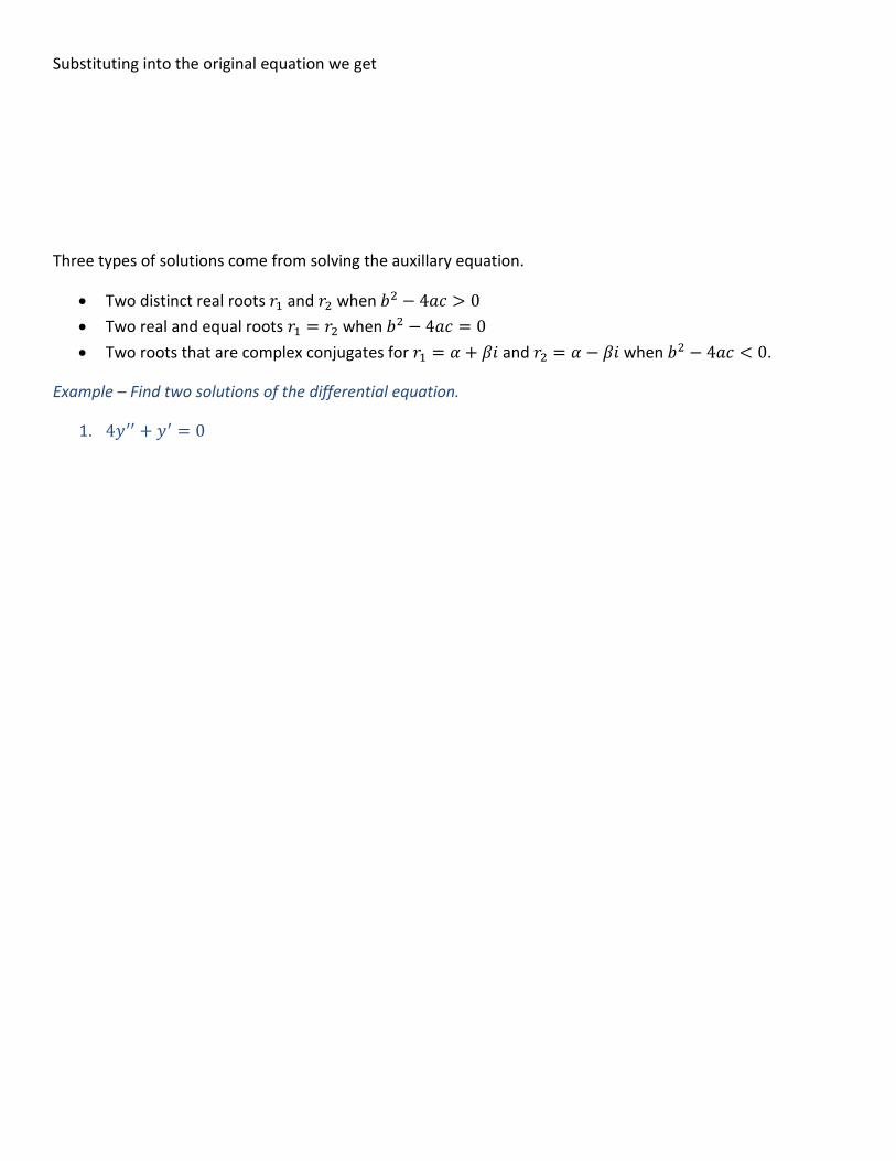
Three types of solutions come from solving the auxillary equation.

Two distinct real roots 𝑟1 and 𝑟2 when 𝑏2 − 4𝑎𝑐 > 0

Two real and equal roots 𝑟1 = 𝑟2 when 𝑏2 − 4𝑎𝑐 = 0

Two roots that are complex conjugates for 𝑟1 = 𝛼 + 𝛽𝑖 and 𝑟2 = 𝛼 − 𝛽𝑖 when 𝑏2 − 4𝑎𝑐 < 0.

Example – Find two solutions of the differential equation.

1. 4𝑦′′ + 𝑦′ = 0

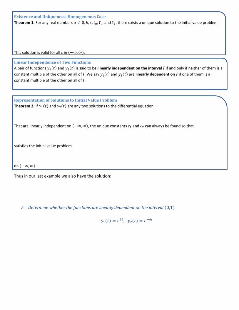
Existence and Uniqueness: Homogeneous Case

Theorem 1. For any real numbers 𝑎 ≠ 0, 𝑏, 𝑐, 𝑡0, 𝑌0, and 𝑌1, there exists a unique solution to the initial value problem

This solution is valid for all 𝑡 in (−∞, ∞).

Linear Independence of Two Functions

A pair of functions 𝑦1(𝑡) and 𝑦2(𝑡) is said to be linearly independent on the interval 𝑰 if and only if neither of them is a

constant multiple of the other on all of 𝐼. We say 𝑦1(𝑡) and 𝑦2(𝑡) are linearly dependent on 𝑰 if one of them is a

constant multiple of the other on all of 𝐼.

Representation of Solutions to Initial Value Problem

Theorem 2. If 𝑦1(𝑡) and 𝑦2(𝑡) are any two solutions to the differential equation

That are linearly independent on (−∞, ∞), the unique constants 𝑐1 and 𝑐2 can always be found so that

satisfies the initial value problem

on (−∞, ∞).

Thus in our last example we also have the solution:

2. Determine whether the functions are linearly dependent on the interval (0,1).

𝑦1(𝑡) = 𝑒3𝑡, 𝑦2(𝑡) = 𝑒−4𝑡

A Condition for Linear Dependence of Solutions

Lemma 1. For any real numbers 𝑎 ≠ 0, 𝑏 and 𝑐, if 𝑦1(𝑡) and 𝑦2(𝑡) are any two solutions to

And

Holds at any point 𝜏, then 𝑦1 and 𝑦2 are linearly dependent on (−∞, ∞).

Note: This is called the Wronskian of 𝑦1 and 𝑦2 and can be expressed as the determinant of a 2 x 2 matrix.

Thus if 𝑦1(𝑡) and 𝑦2(𝑡) are linearly independent, then we say the general solution is

Distinct real roots: If the auxiliary equation has two distinct roots 𝑟1 and 𝑟2, then the general solution is

Repeated roots: If the auxiliary equation has one repeated root 𝑟, then the general solution is

Find the general solution.

3. 𝑦′′ + 5𝑦′ + 6𝑦 = 0

4. 𝑦′′ + 10𝑦′ + 25𝑦 = 0

Solve the initial value problem.

5. 𝑦′′ − 4𝑦′ + 3𝑦 = 0 ; 𝑦(0) = 1 , 𝑦′(0) = 1 3⁄

4.3 Auxiliary Equations with Complex Roots

In this section we will look at differential equations with constant coefficients

Where the auxiliary equation

has two complex roots

where 𝛼 and 𝛽 > 0 are real and 𝑖2 = −1.

These roots would yield us the solutions

Using Euler’s Formula, 𝑒𝑖𝜃 = cos 𝜃 + 𝑖 sin 𝜃, we can manipulate the above solution to get

Examples

1. 𝑦′′ − 6𝑦′ + 10𝑦 = 0

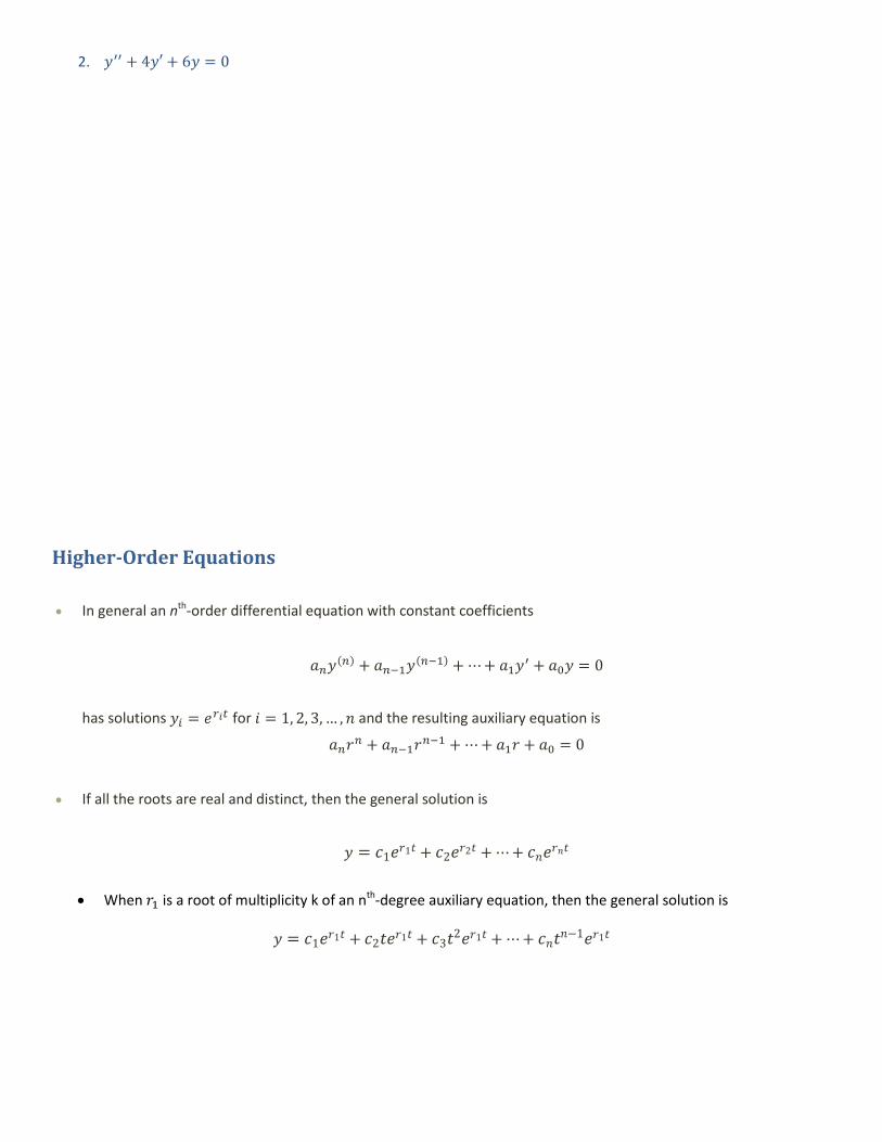
2. 𝑦′′ + 4𝑦′ + 6𝑦 = 0

Higher-Order Equations

In general an nth-order differential equation with constant coefficients

𝑎𝑛𝑦(𝑛) + 𝑎𝑛−1𝑦(𝑛−1) + ⋯ + 𝑎1𝑦′ + 𝑎0𝑦 = 0

has solutions 𝑦𝑖 = 𝑒𝑟𝑖𝑡 for 𝑖 = 1, 2, 3, … , 𝑛 and the resulting auxiliary equation is

𝑎𝑛𝑟𝑛 + 𝑎𝑛−1𝑟𝑛−1 + ⋯ + 𝑎1𝑟 + 𝑎0 = 0

If all the roots are real and distinct, then the general solution is

𝑦 = 𝑐1𝑒𝑟1𝑡 + 𝑐2𝑒𝑟2𝑡 + ⋯ + 𝑐𝑛𝑒𝑟𝑛𝑡

When 𝑟1 is a root of multiplicity k of an nth-degree auxiliary equation, then the general solution is

𝑦 = 𝑐1𝑒𝑟1𝑡 + 𝑐2𝑡𝑒𝑟1𝑡 + 𝑐3𝑡2𝑒𝑟1𝑡 + ⋯ + 𝑐𝑛𝑡𝑛−1𝑒𝑟1𝑡

Examples – Find the general solution.

6. 𝑦′′′ + 5𝑦′′ + 3𝑦′ + 9𝑦 = 0

7.

26𝑑4𝑦

𝑑𝑥4+ 24

𝑑2𝑦

𝑑𝑥2+ 9𝑦 = 0

4.5 The Superposition Principle

Superposition Principle Theorem 3. Let 𝑦1 be a solution to the differential equation

And 𝑦2 be a solution to

Then for any constants 𝑘1 and 𝑘2, the function 𝑘1𝑦1 + 𝑘2𝑦2is a solution to the differential equation

Example

1. Given that 𝑦𝑝1= 3𝑒2𝑥 and 𝑦𝑝1

= 𝑥2 + 3𝑥 are particular solutions to

𝑦′′ − 6𝑦′ + 5𝑦 = −9𝑒2𝑥 𝑎𝑛𝑑 𝑦′′ − 6𝑦′ + 5𝑦 = 5𝑥2 + 3𝑥 − 16

respectively, find a particular solution to

a. 𝑦′′ − 6𝑦′ + 5𝑦 = 5𝑥2 + 3𝑥 − 16 − 9𝑒2𝑥

b. 𝑦′′ − 6𝑦′ + 5𝑦 = −10𝑥2 − 6𝑥 + 32 + 𝑒2𝑥

Existence and Uniqueness: Nonhomogeneous Case Theorem 4. For any real numbers 𝑎 ≠ 0, 𝑏, 𝑐, 𝑡0, 𝑌0, and 𝑌1, suppose 𝑦𝑝(𝑡) is a particular solution to the

nonhomogeneous differential equation

In an interval 𝐼 containing 𝑡0 and that 𝑦1(𝑡) and 𝑦2(𝑡) are linearly independent solutions to the associated

homogeneous equation

In 𝐼. Then there exists a unique solution in 𝐼 to the initial value problem

And it is given by

For the appropriated choice of the constants 𝑐1 and 𝑐2.

Example

1. Find the general solution

𝑦′′ − 𝑦′ − 2𝑦 = 1 − 2𝑡 , 𝑦𝑝(𝑡) = 𝑡 − 1

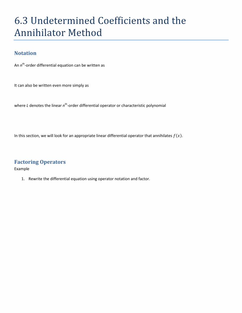
6.3 Undetermined Coefficients and the Annihilator Method

Notation

An nth-order differential equation can be written as

It can also be written even more simply as

where L denotes the linear nth-order differential operator or characteristic polynomial

In this section, we will look for an appropriate linear differential operator that annihilates 𝑓(𝑥).

Factoring Operators Example

1. Rewrite the differential equation using operator notation and factor.

Annihilator Operators If L is a linear differential operator with constant coefficients and f is a sufficiently differentiable function such that

then L is said to be an annihilator of the function.

Examples – Find the differential operator that annihilates each function.

2. 𝑦 = 𝑘

3. 𝑦 = 𝑥

4. 𝑦 = 𝑥4

The function 𝑥𝑛 is annihilated by the differential operator

Note: This annihilator will also annihilate any linear combination of these functions:

The function 𝑥𝑛𝑒𝛼𝑥 is annihilated by the differential operator

If 𝐿1 annihilates 𝑦1(𝑥) and 𝐿2 annihilates 𝑦2(𝑥), then the product of the differential operators 𝐿1 ∙ 𝐿2 will annihilate the

linear combination

Note: The differential operator that annihilates a function is not unique.

Example

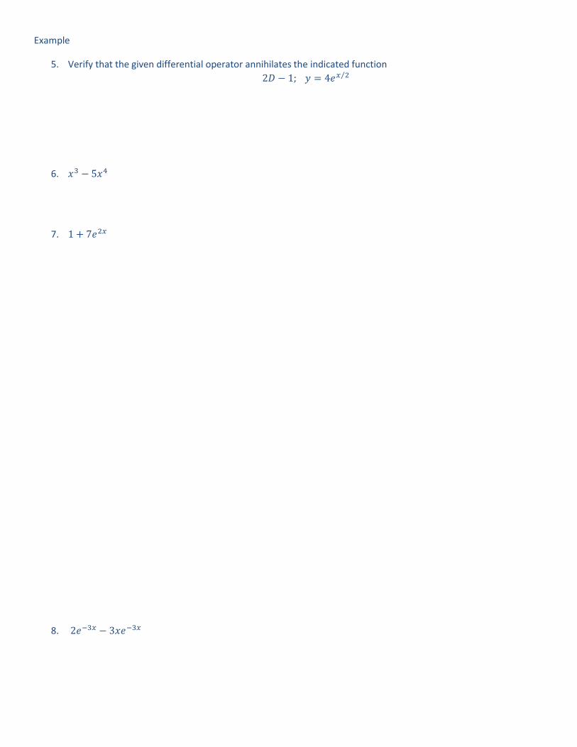
5. Verify that the given differential operator annihilates the indicated function

2𝐷 − 1; 𝑦 = 4𝑒𝑥 2⁄

6. 𝑥3 − 5𝑥4

7. 1 + 7𝑒2𝑥

8. 2𝑒−3𝑥 − 3𝑥𝑒−3𝑥

The functions 𝑥𝑛𝑒𝛼𝑥 cos 𝛽𝑥 and 𝑥𝑛𝑒𝛼𝑥 sin 𝛽𝑥 are annihilated by the differential operator

Special Case: when 𝛼 = 0 and 𝑛 = 0, then

Example

9. 1 + sin 𝑥

10. 8𝑥 − sin 𝑥 + 10 cos 5𝑥

Method of Undetermined Coefficients: Annihilator

1. Solve the associated homogeneous equation to find 𝑦𝑐.

2. Find the annihilator for 𝑔(𝑥) and apply it to both sides of the differential equation.

3. Solve the now homogeneous DE to find the general solution.

4. Identify the particular solution, 𝑦𝑝, and find its derivatives.

5. Plug 𝑦𝑝 and its derivatives into the original equation to find the unknown constant.

Examples – Solve

11. 𝑦′′ − 3𝑦′ − 4𝑦 = 3𝑒2𝑥

12. 𝑦′′ + 4𝑦 = 4 cos 𝑥 + 3 sin 𝑥 − 8

4.6 Variation of Parameters

Cramer’s Rule The solution to a system of equations

Is given by

Solving Second-Order DE’s

For a second-order DE of the form

Where the solution to the related nonhomogeneous equation is

Can we vary the paramters of 𝑐1 and 𝑐2 to be function 𝑢1(𝑥) and 𝑢2(𝑥)?

Let a particular solution be

Where 𝑦1 and 𝑦2 form a fundamental set of solutions on I of the associated homogeneous equation.

Then

And

Substituting into our DE 𝑦′′ + 𝑃(𝑥)𝑦′ + 𝑄(𝑥)𝑦 = 𝑓(𝑥)

And after a lot of simplification, we get

𝑑

𝑑𝑥[𝑢1

′ 𝑦1 + 𝑢2′ 𝑦2] + 𝑃[𝑢1

′ 𝑦1 + 𝑢2′ 𝑦2] + 𝑢1

′ 𝑦1′ + 𝑢2

′ 𝑦2′ = 𝑓(𝑥)

In order to come up with a system of equations to solve for 𝑢1′ and 𝑢2

′ we will make the assumption that

𝑢1′ 𝑦1 + 𝑢2

′ 𝑦2 = 0

Which gives us a second equation

𝑢1′ 𝑦1 + 𝑢2

′ 𝑦2 = 𝑓(𝑥)

This system of equations can be solved using Cramer’s Rule and gives us

Where

Method of Variation of Parameters 1. For a given equation

Find the complementary function

2. Compute the Wronskian 𝑊(𝑦1(𝑥), 𝑦2(𝑥))

3. Put the DE in standard form by dividing by 𝑎2

4. Find 𝑢1 and 𝑢2 from

5. Then

and the general solution is

Examples – Solve.

1. 𝑦′′ + 𝑦 = sec 𝑥

2.

𝑦′′ − 9𝑦 =9𝑥

𝑒3𝑥

Third- Order Equations

When 𝑛 = 3,

Where 𝑦1, 𝑦2, and 𝑦3 are a linearly independent set of solutions of the associated homogeneous DE and 𝑢1,

𝑢2, and 𝑢3 are determined by

Higher-Order Equations For a n

th-order DE in standard form

The complementary function is

The particular solution is

And Cramer’s Rule gives us

4.7 Variable Coefficient Equations

Existence and Uniqueness of Solutions

Theorem 5. Suppose 𝑝(𝑡), 𝑞(𝑡), and 𝑔(𝑡) are continuous on an interval (𝑎, 𝑏) that contains the point 𝑡0.

Then, for any choice of the initial values 𝑌0 and 𝑌1, there exists a unique solution 𝑦(𝑡) on the same interval

to the initial value problem

Example 2.

𝑥𝑑𝑦

𝑑𝑥= 𝑦, 𝑦(0) = 1

The Cauchy-Euler Equations

A linear second-order differential equation that can be expressed in the form

Where 𝑎, 𝑏, and 𝑐 are constants, is called a Cauchy-Euler, or equidimensional, equation.

Notice the exponent of the variable coefficient matches the degree of the derivative for each term.

Solving a Cauchy-Euler Equation

Given an homogeneous second-order DE

In Section 4.3 we let 𝑦 = 𝑒𝑟𝑡, for a Cauchy-Euler Equation let 𝑦 = 𝑡𝑟

Thus 𝑦 = 𝑡𝑟 is a solution of the differential equation whenever r is a solution to the auxiliary equation

As in Section 4.2, there are three types of solutions come from solving the auxiliary equation.

Two distinct real roots 𝑟1 and 𝑟2 when 𝑏2 − 4𝑎𝑐 > 0

o General Solution:

Two real and equal roots 𝑟1 = 𝑟2 when 𝑏2 − 4𝑎𝑐 = 0

o General Solution:

Two roots that are complex conjugates for 𝑟1 = 𝛼 + 𝛽𝑖 and 𝑟2 = 𝛼 − 𝛽𝑖 when 𝑏2 − 4𝑎𝑐 < 0.

o General Solution:

Example – Solve.

1. 2𝑥2𝑦′′ + 𝑥𝑦′ − 𝑦 = 0

2. 4𝑥2𝑦′′ + 𝑦 = 0

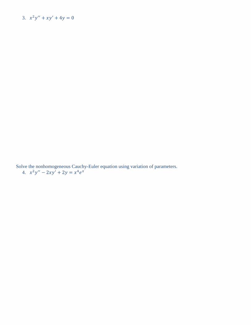
3. 𝑥2𝑦′′ + 𝑥𝑦′ + 4𝑦 = 0

Solve the nonhomogeneous Cauchy-Euler equation using variation of parameters.

4. 𝑥2𝑦′′ − 2𝑥𝑦′ + 2𝑦 = 𝑥4𝑒𝑥