Embed Size (px)
Citation preview

249VOLUME V / INSTRUMENTS
4.3.1 Introduction
Rheology is one of the few branches of science with aprecise ‘birthday’, April 29, 1929, the date when theRheology Society was founded in Columbus, Ohio thanks tothe initiative of a group of scientists, including Eugene C.Bingham, Wolfgang Ostwald, Ludwig Prandtl, and MarkusReiner. On that occasion, Bingham and Reiner invented theword rheology from the Greek verb rew (to flow) in order todescribe the science that studies the flow and deformation ofbodies. The famous expression panta rei by the ancientphilosopher Heraclitus from Ephesus was chosen as themotto of the Rheology Society, while the hourglass wasselected as its symbol.
According to rheology, all real bodies have propertieswhich fall between two extreme ideal behaviours of theperfectly elastic body and the perfectly viscous fluid. In1678, Robert Hooke formulated the law (ut tension sic vis)which states that in an elastic body, deformation g isproportional to imparted stress s (Hooke, 1931)
[1]
Hooke’s law defines the behaviour of the ideal elasticbody. The proportionality constant G is usually called theelastic modulus of the material. Since g is an adimensionalnumber, both s and G have the same dimensions for a forceapplied over a surface, expressed in Pa in the InternationalSystem of Units.
At the opposite extreme of material behaviour,perfectly viscous fluids can be found. Applying stress ona viscous fluid generally produces a motion whichcontinues until the stress is removed. Consider twoparallel surfaces, each having an area A at a reciprocalsmall distance d with a fluid interposed in between asshown in Fig. 1. A shear force per unit surface sFAapplied to the upper surface makes it move at constantvelocity U. If the second surface is still, a velocitydifference is then created in the fluid, that shifts from Uto zero. In 1687, Isaac Newton stated that aproportionality relationship exists between s called shearstress, and the velocity gradient U/d (Newton, 1999). Thelatter is represented with g
.and is also called shear
deformation velocity. The relationship
[2]
is the equation which describes Newtonian fluids and theproportionality constant h is usually called viscosity,sometimes with the adjective dynamic, in order todistinguish it from the kinematic viscosity n, defined by theratio hr, where r is the fluid density. In the InternationalSystem of Units, g
.is expressed in s1, h is expressed in
Pas, and n in m2s1.Linear equations [1] and [2], resulting from the
mathematical modelling of two ideal extreme cases, providestress-deformation-time relationships, and representexamples of constitutive equations. For many years, theywere considered universal laws, although experimentalobservations pointing out exceptions were revealed inscientific publications of the Nineteenth century.
Newtonian fluid mechanics, like the classical theory ofelastic bodies, is not usually considered a part of the specificfield of rheology, which, in fact, deals with the behaviour ofviscoelastic bodies that usually have intermediatecharacteristics with respect to the two ideal extreme casesdescribed above.
In order to describe viscoelasticity, it is not necessary,however, to remove the linearity hypothesis characterizingthe laws dictated in equations [1] and [2]. Equation
[3]
is a linear constitutive equation of a body possessingsimultaneously both elastic and viscous characteristics.Linear models are capable of describing several types of
σ γ ηγ= +G
σ ηγ=
σ γ=G
4.3
Rheology
FA
U
x
d y
Fig. 1. Velocity field for a viscous fluid between two parallel surfaces (relative velocity U).

rheologic behaviour and are therefore extremely useful (seebelow). However, they can usually be considered valid onlyfor small variations of g and g
.in a regime that is, in fact,
called linear, where G and h are generally the functions of gand g
..
The concept of viscoelasticity introduces a certainambiguity with respect to the most elementaryclassifications used to define the state of materials. Thedistinction between solid and liquid is not entirely clearsince the same body can show characteristics that areprevalently solid or liquid, depending on the type of stressthat is applied to it. This issue can be considered fromanother point of view. In 1964, M. Reiner introduced anadimensional parameter called the Deborah number
[4]
defined as the ratio between a characteristic time t of thematerial and a characteristic time T of the observation. Athigh Deborah numbers, the behaviour of the body isprevalently solid, while at low Deborah numbers, thebehaviour is essentially liquid. A material, then, canbehave as a solid either because it has a very highcharacteristic time or because the deformation processused to study its characteristics is very fast. On the otherhand, a material can display an ability to flow if it has alow characteristic time or if the observation time is longenough. Polymeric melts, for instance, have rather longrelaxation times, in the order of 1-100 s, and very oftenthey can be treated as elastic bodies in practical problems.Many materials have characteristic times around 1 s andtherefore, in our daily experience, they seem likeviscoelastic bodies.
The Deborah number takes its name from the Biblicalprophetess Deborah to whom these words are attributed:“[…] and mountains flowed in front of God”. Inparaphrasing this expression, it is possible to suppose that ifsufficient observation time were available, one would seeeven mountains flow. As a matter of fact, it has beenobserved that the thickness of one-thousand-year-oldwindows in gothic churches is slightly thicker in the lowerpart, which demonstrates that there was a flow from theupper to the lower parts as an effect of gravity.
In general, in order to adequately describe the state ofstress on a body, it is necessary to introduce the so-calledstress tensor. If one considers an elementary cube of unitvolume, and taking the x, y and z axes parallel to the cubeedges, the stress tensor is defined as follows:
[5]
The components acting in a direction normal to the facesof the cube have the first and the second index equal to eachother, while tangential components have different indexes.The first index refers to the direction normal to the plane onwhich the stress is acting, while the second refers to thedirection of the stress. Likewise, it is possible to describe thestate of deformation eij, which represents the dimensionalvariations of the cube divided by its initial dimensions. Thetensor of the velocities of deformation vij is also defined inthe same way. The usefulness of this type of notation can beimmediately understood by observing that the shear flux
used above to describe the Newton postulate (see Fig. 1),conveniently described as follows:
[6]
In the case of a Newtonian fluid undergoing the fluxdescribed in [6], the stress distribution is:
[7]
4.3.2 Viscosity
The concept of viscosity was previously introduced,retaining Eq. [2] as its definition. However, viscosity isconstant only for Newtonian fluids when the sheardeformation velocity g
.varies. Table 1 shows the order of
magnitude of viscosity in a series of materials of commonuse. In general, the viscosity of real materials does not onlydepend on g
., but also on temperature T and pressure p, and it
can also depend on the material’s history of deformation. Forall liquids, the viscosity decreases with increasingtemperatures and decreasing pressure. This dependency, atlow shear, is well described by the following empiricalrelationship:
[8]
Typical b values range from 0.03 K1 forpolyolephines to 0.1 K1 for polystyrene, while a1–4kbar1 for the same materials. The viscosity-temperaturecorrelation in non-Newtonian fluids is often morecomplex. In rheological measurements, it is thereforeextremely important to control the temperature, takinginto consideration the fact that a stress factor within amaterial can generate heat. Less significant, and usuallyneglected, is the effect of pressure.
A major aspect of rheology is the study of viscosityvariations of fluids as a function of g
.. The problem is
important from a practical point of view, since significantlydifferent g
.values can correspond to the different
η0 1= −K e ebT ap
σ σ σ σxx yy yy zz− = − =,0 0σ ηγ σ σyx xz yz= = =, ,0
v v vxx yy zz= = =γ , 0
σ
σ σ σ
σ σ σ
σ σ σij
xx xy xz
yx yy yz
zx zy zz
=
De T=τ
FLUID MOTION
250 ENCYCLOPAEDIA OF HYDROCARBONS
Table 1. Viscosity of some commonly used materialsat room temperature
Material Approximated viscosity [Pas]
Glass 1040
Melted glass (500°C) 1012
Bitumen 108
Melted polymers 103
Cane syrup 102
Liquid honey 101
Glycerol 100
Olive oil 101
Water 103
Air 105

technological processes as reported in Table 2. Variousrheological behaviours can be elicited from the samematerial depending on the field of g
.it is subject to. For
instance, paint must have sufficiently high viscosity at low g.
values (102–101 s1) in order for it not to sag once it isapplied to a wall. At the same time, for the paint to be easilyapplied, its viscosity should be quite low when is around101–102 s1.
Figure 2 shows the most typical fluid behaviours,illustrated by curves on a s-g
.graph. Viscosity is given by the
slope of these curves (hds/dg.). A Newtonian fluid is
represented by a straight line passing through the origin; azero velocity corresponds to zero stress. A second type offluid is represented having a constant viscosity but whichrequires minimum stress to start flowing. These are the so-called Bingham fluids, represented in Fig. 2 by a straightline which does not pass through the origin, but interceptsthe y axis at the s0 value called the yield point. In Fig. 2, thetypical curves of pseudoplastic fluids are also representedwith viscosity decreasing with increasing stress, whereas thecurves of the dilatant fluids show viscosity increasing withincreasing stress. A last type of behaviour shown in Fig. 2 is
RHEOLOGY
251VOLUME V / INSTRUMENTS
˙
pseudoplastic withyield point
pseudoplastic
Newtonian
shear thickening
Bingham
g
so
so
sFig. 2. Shear stress s - shear rate
.g graph
for different kinds of fluids.
Table 2. Typical rates of deformation for some processes
Process Rate of deformation [s1] Application
Sedimentation of fine powderin a suspending liquid 106-104 Pharmaceuticals, paint
Leveling due to surface tension 102-101 Paint, ink
Draining due to gravity 101-101 Paint, coatings
Extrusion 100-102 Polymers
Mastication 101-102 Food
Coating by immersion 101-102 Paint, enamels, sweets
Mixing and agitation 101-103 Manufacturing of liquid materials
Flowing in a tube 100-103 Pumping, blood flow in veins
Spraying 103-104 Atomization, spray-drying
Brushing 103-104 Paint
Rubbing 103-104 Application of creams on skin
Pigment grinding in a base fluid 103-105 Paint, ink
High speed coating 105-106 Paper industry
Lubrication 103-107 Motors

that of pseudoplastic fluids with a yield point, represented ona s-g
.graph by a curve with a decreasing slope and
intercepting the y axis at a s0 value.Most fluids of practical interest are pseudoplastic which
is why rheology dedicates special attention to them. Apossible behaviour of a pseudoplastic fluid is shown in Fig. 3where the same experimental data are reported in threedifferent ways: a h viscosity curve as a function of the shearstress s (Fig. 3 A) a curve showing s as a function of thevelocity of deformation g
.(Fig. 3 B), and a h curve as a
function of g.
(Fig. 3 C). Notice that the h(s) curve shows theexistence of two plateaus at low and high s values where theviscosity varies very little, usually called the first Newtonianregion, and the second Newtonian region. The variation of hat intermediate values of s is much faster, however. Thevalue of viscosity in the first Newtonian region is oftenreferred to as viscosity at zero stress, indicated by h0,whereas the value in the second Newtonian region is calledviscosity at infinite stress. These values are obviouslyextrapolations since there is no experimental method capableof performing measurements at zero or infinite stress. Notice
also in Fig. 3 that it appears as though the fluid does notreally present a yield value. However, if measurements wereperformed in a g
.field between 101 and 104 s1, the
conclusion would be different, as observed in the s(g.) graph,
where the dashed portion of the curve represents thebehaviour of an ideal Bingham fluid. But then, Binghamfluids by definition have infinite viscosity at low shear, andtherefore they do not display a Newtonian plateau. Theconcept of yield has a certain practical importance, but thenew generation of rheometers, which can measure extremelylow stress, has questioned its veracity (Barnes and Walters,1985). It has been experimentally demonstrated thatBingham materials exhibit very high viscosity variations (upto 6 orders of magnitude) for small stress variations andfinite viscosity which are very high in relation to low stress.
Several equations have been suggested to describe thegeneral form of the h(g
.) curves. Usually these equations
contain at least four parameters which are essentiallyempirical, even if microstructural explanations wereattempted, with probably the best known being the Crossequation (1965):
[9]
where h0 and h are the asymptotic values of viscositypreviously introduced. K and m are two parameters; the firstwith dimensions of time while the second is adimensional.Alternatives to the Cross equation were suggested, amongwhich the Carreau model (1972) is worth mentioning.Thereare also some useful approximations of the Cross model, theforemost being applied when hh0 and hh, where [9]can be written as:
[10]
which with redefined parameters can be written as follows:
[11]
Equation [11] is a widely used power law whichdescribes the behaviour of several polymeric solutions quitewell. Furthermore, when n1, then [11] models aNewtonian fluid, and when n1, it can describe a dilatantsystem. However, when hh0 then the Cross equation canbe simplified as follows:
[12]
This last equation is known as the Sisko model (1958).When n0, the equation is expressed as:
[13]
This is the so-called Bingham model which describes thefluids by the same name, where s0 is the yield valueintroduced above and hp is the plastic viscosity, bothconstant. In general, the equations reported above describethe behaviour of different systems, but usually only inlimited fields of variation of g
..
Dilatant fluids are much less common than pseudoplasticfluids. Dilatant effects are usually due to the phenomena ofstructure organization within the fluid at high shear rates. Aspointed out above, the flow curves of dilatant fluids can bedescribed by power laws.
It is a common occurrence for the rheological behaviourof a fluid to display some time dependency effects. By
σ σ η γ= +0 p
η η γ= +∞−K n
11
η γ= −K n1
1
η ηγ
=( )
0
K m
η ηη η γ−−
=+( )
∞
∞0
11 K m
FLUID MOTION
252 ENCYCLOPAEDIA OF HYDROCARBONS
g (s1)
A
B
C
˙
g (s1)
s (Pa)
˙
s (
Pa)
h (
Pa. s
)h
(Pa
. s)
105
103
101
101
105
103
101
101
103
101
101
104106 104 102 100 102
104106 104 102 100 102
103101 100 101 102
Fig. 3. Behaviour of a pseudoplastic fluid represented in three different ways: A, as a graph of viscosity h as a function of shear stress s; B, as a graph of s as a function of shear
.g,
where the dashed line represents ideal Bingham behaviour; C, as a graph of h as a function of
.g
(Barnes et al., 1989).

applying a constant stress, it is possible that the viscositymay increase, in which case the fluid is called reopectic. Butthe most common case is a decrease in the viscosity in whichthe fluid is called thixotropic. Practically speaking, it isdifficult to discriminate between thixotropic andpseudoplastic fluids because the effects of time and velocityoften overlap in experimental measurements making itdifficult to tell them apart. Moreover, many materials areboth thixotropic and pseudoplastic. A rather useful way tocharacterize thixotropic fluids is by reporting theviscosity-time curve in two phases: first under the action ofa constant stress and then at zero stress. When stress isapplied, initially the viscosity grows abruptly, but then itdecreases until it reaches a constant value. When the stressstops, the viscosity almost instantaneously increases, andthen increases more slowly, asymptotically approaching itsoriginal value.
Thixotropic and reopectic behaviours derive from thefact that a stress factor can provoke irreversiblemodifications in the material (such as crosslinking,coagulum formation, degradation, and mechanic instability),or reversible modifications (breakage and new formation ofcolloidal aggregates or networks). Models proposed todescribe the behaviour of reopectic and thixotropic systemsare much less satisfactory than those proposed to describepseudoplasticity. For more in-depth information, see thepublication by Barnes, 1997.
4.3.3 Normal stresses, elongationalviscosity
In non-Newtonian fluids, shear stresses can also generatenon-isotropic components of normal stresses. This means, inreference to the stress tensors defined in [5], that normalcomponents sxx, syy, szz are not zero. The insurgence ofnormal stresses has some easily observable consequences,some of which are quite spectacular. The best known iscertainly the phenomenon called the Weissenberg effect: aNewtonian fluid mixed in a cylindrical vessel by acylindrical pole is pushed towards the walls of the vessel bycentrifugal force, and its surface assumes a parabolic profilewith a minimum quantity of fluid near the pole while, on thecontrary, a viscoelastic fluid tends to rise along the pole. Thestress distribution in a non-Newtonian fluid can be describedas follows:
[14]
where s, N1 and N2 are sometimes called viscosimetricfunctions, while N1 and N2 are usually called, the first andsecond normal stress differences, respectively. It is oftenpossible to describe N1 with a power law:
[15]
It is quite common for the first normal stress difference,N1, to have a higher value than the s stress, itself. The ratiobetween N1 and s can be considered an indication of theelasticity of the fluid. On the other hand, the seconddifference, N2, is usually small, compared to N1. There is aparticular class of fluids, including the so-called Bogerfluids, where N20. Boger fluids are mostly very diluted
solutions ( 0.1%) of a high molecular weight polymer in avery viscous solvent.
In many manufacturing operations using polymericmaterials, there exists a significant elongational flowcomponent. For instance, spinning exerts a lengthening inthe fibre direction, and a film blowing operation causes alengthening in the machine direction and in the directiontangential to the bubble. Elongational flow was not givenmuch attention until the mid-1960’s, but subsequently, itsimportance became clear, particularly the enormousdifferences between Newtonian fluids and elastic non-Newtonian fluids. A melted polymer of length L, constrainedat one end and subjected to traction in direction x, has zerovelocity at the point of constraint, and is equal to
.e at the end
where the force is applied. In intermediate positions,between 0 and L, the equation is:
[16]
In perpendicular directions, if the fluid is incompressibleand the Poisson coefficient is equal to 12, it is:
[17]
The corresponding stress distribution is:
[18]
where hE represents the uniaxial extensional viscosity. Ingeneral, hE depends on the uniaxial deformation velocity
.e,
as occurs for shear viscosity, but the type of functionaldependency is usually different for each of them. It is quitecommon that a polymer, the shear viscosity of whichdecreases when
.g increases, shows extensional viscosity
increasing with the increase of.e.
For Newtonian fluids, Frederick Thomas Trouton in 1906obtained:
[19]
For the Trouton ratio defined as:
[20]
Jones et al. (1987) proposed the following equation:
[21]
Shear viscosity is evaluated at a shear deformationvelocity that is numerically equal to
2
3.e.
4.3.4 Rheometric measurements
Several methods have been devised to measure viscosity andmany commercial instruments are capable of covering widefields of viscosity and velocity gradients. Specific criteriashould be considered when choosing an instrument related toa series of properties of the material that must be analyzed,namely its physical nature, the order of magnitude of itsviscosity, its elasticity, the dependency of viscosity ontemperature, just to mention a few.
The early viscosimeters were usually capable ofproviding measurements for a single value of the velocity ofdeformation. Today, some of these viscosimeters survive as
Tr E
ε η ε
η ε( )= ( )
( )3
Tr E= ( )( )
η εη γ
η ηE = 3
σ σ σ σ εη ε
σ σ σxx yy xx zz E
xy xz yz
− = − = ( )= = =
0
v y v zy z=− =− ε ε2 2;
vL
xx =ε
N A m1 = γ
σ σ η γ γ σ σ
σ σ γ σ
= = ( ) = =
− = ( ) −yx xz yz
xx yy yyN
, ,
,
0
1 σσ γzz N= ( )2
RHEOLOGY
253VOLUME V / INSTRUMENTS

quality control instruments at the industrial level, butevidently, based on the information in the previousparagraph, one-point measurements provide very incompleteand sometimes even misleading descriptions for thebehaviour of material. In general, viscosimeters can beclassified as three different types: capillary, rotational, andwith a mobile body.
Capillary viscosimeters were the first to be conceivedand they are still very popular today: the fluid is somehowforced to flow through a capillary tube and its viscosity isdetermined by measuring its efflux velocity. TheHagen-Poiseuille equation is commonly used for thispurpose (in hypothesis of steady, laminar and isothermalflow):
[22]
where r is the capillary radius, p is the pressure drop in thecapillary, V is the volume of liquid flowing during time t.Capillary viscosimeters are particularly useful to preciselymeasure fluid viscosity for values up 20 Pas. Shear ratesthat can be obtained in such an instrument can be verydifferent, depending on the fluid. For a Newtonian fluid,
.g
varies from a value at the wall .gw equal to:
[23]
where Q represents the volumetric flow, to a value equal tozero at the center of the tube. The stress at the wall sw is
[24]
In the case of a non-Newtonian fluid, on the other hand,the following expression is derived:
[25]
whereas the stress at the wall sw does not vary with respectto the value given in [24]. The term between parentheses in[25] is called the Rabinowitsch correction. Thus it is finallypossible to derive:
[26]
Since the pressure drop is usually measured between areservoir above the capillary and the atmosphere below it, itis also necessary to account for the pressure drop related tothe entrance of the fluid into the capillary and its exittowards the atmosphere. While the second factor is usuallynegligible, the first is often important and it should becorrectly accounted for.
There are several different types of instruments whichapply the concept of capillary viscosimetry. For instanceseveral glass capillary viscosimeter models have beendeveloped where the fluid flows when pushed by thehydrostatic head, providing the means to directly measurethe kinematic viscosity of Newtonian fluids as long astheir viscosity is not too high. However, in some models itis also possible to apply an external pressure so that thenon-Newtonian behaviour can also be studied. In general,however, glass capillary viscosimeters can only produce
low shear rates. Then there are also the so-called orificeviscosimeters, a very simple tool commonly used onlyduring the phase of production control for paint, ink,adhesives and lubricant oils. They consist of a vessel onthe bottom of which a capillary hole has been opened. Inthis case the time necessary to empty the vessel ismeasured, but obviously here the hydrostatic head is notconstant over time, and significant kinetic effects occur.Moreover, the flux does not satisfy the Hagen-Poiseuilleequation as it is quite complex and not simply and directlylinked to viscosity. This type of measurement can be usedto compare different fluids, but it cannot express aviscosity. Finally, there are the so-called extrusionviscosimeters that are more specifically used forpolymeric melts. They consist of a reservoir connected toa capillary tube: the fluid is forced out by a piston onwhich a constant force is applied.
Rotational viscosimeters are usually separated into twoportions by the fluid to be analyzed. The two portions canconsist of two concentric cylinders, two plates, a cone and aplate, or an impeller inside a cylinder. The relative rotationof the two parts produces shear. The torque required toproduce a certain angular viscosity, or the angular viscositynecessary to produce a certain torque representmeasurements of viscosity. Rotational viscosimeters aregenerally more flexible than capillary viscosimeters, as theyperform measurements on a wide variety of fluids with verydifferent viscosities in a wide range of velocity gradients.Therefore, they represent optimal instruments to study thenon-Newtonian character of fluids and potential thixotropicor reopectic effects.
The most common type of rotational viscosimeter hasconcentric cylinders. If the distance between the twocylinders is sufficiently small, and the two cylinders movewith relative motion, then the fluid between them undergoesa constant shear rate. In particular, by indicating the cylinderradii with r0 and r1, and the angular velocity of the internalcylinder (while the external cylinder does not move) withW1, the shear rate
.g is given by:
[27]
whereas the stress is
[28]
where C is the value of the applied torque, and L is theheight of the fluid between the two cylinders. From [27] and[28], the following expression for viscosity is derived:
[29]
Equation [29], however, is valid only for very smalldistances, i.e. when the br0r1 ratio is higher than 0.97, acondition which is not easy to obtain due to the difficulty inaligning the two cylinders. Some viscosimeters useconcentric cylinders systems with larger distances, but it ismore complicated to derive the viscosity equation in theseconditions. The problem was solved by Krieger and Maron(1954), who assumed that in the measurement interval, theshear rate and shear stress were related by a power law suchas in [11], and derived the expression of the shear rate at theinternal cylinder as follows:
η =−( )C r r
r L0 1
0
3
12π Ω
σ = Cr L2 0
2π
γ =−
rr r
0 1
0 1
Ω
η γσγ
σ
w
w
w
w
a p L
Q d Qd
( ) = =( )+
π 4
83
4
1
4
∆
ln
ln
γσw
w
Qr
d Qd
= +
4 34
143π
lnln
σ w
r pL
= ∆2
γwQr
=4
3
π
η = πr t pV
4
8
∆
FLUID MOTION
254 ENCYCLOPAEDIA OF HYDROCARBONS

[30]
While the shear stress is
[31]
The value of n is determined by reporting the experimentalvalues of C as a function of W1 on a graph and by evaluatingthe slope of the curve at the value of W1 under consideration.Viscosity, measured at the internal cylinder shear rate is
[32]
The minimum limit of velocity that can be obtained inconcentric cylinder rheometers is related to the type of motorused. The maximum limit is generally related to the type offluid investigated. The first factor to take into considerationis that of sample heating caused by viscous friction, whichrenders the measurement unreliable when it surpasses acertain level. Moreover, in certain cases circumferential fluxlines can break and therefore vortexes and turbulence canappear, which lead to flux regimes requiring more energy,therefore provoking an increase of apparent viscosity.
Cone and plate geometry is also of great importance; theshear rate is essentially the same throughout the fluid, aslong as the straight and cone angle q0 is small enough asshown by:
[33]
where W1 is the rotational velocity of the plate. Observe that.g does not depend on fluid properties. The stress on the fluidis estimated by measuring the torque C acting on the conerepresented as:
[34]
where a is the radius of the cone. The viscosity is thenexpressed as:
[35]
With respect to concentric cylinder geometry, cone andplate geometry has several advantages: the sampledimensions are smaller, data are easier to convert, and theshear rate in the sample is constant. However, there arepractical problems that must be considered, such as thepossibility of solvent evaporation and the fact that thesample must be accurately positioned so that the geometry iscompletely filled but not covered.
Another widely used method is parallel plate geometry.The main advantage of this geometry is the possibility offreely varying distance h which separates the two plates; this isparticularly important when studying suspensions containingrather large particles. A general rule in obtaining reproduciblemeasurements is to keep the plate distance at one order ofmagnitude higher than the maximum aggregate size present inthe suspension. In parallel plate geometry, however, the shearrate is not constant, but increases as the distance from thecenter of the plates increases. Maximum velocity is thenobtained at the rim of the plate (for ra) and it is equal to:
[36]
The expression that allows us to estimate the viscosity ismore complicated in this case, derived by Ken Walters (1975)
[37]
4.3.5 Linear viscoelasticity
Viscoelasticity, as mentioned in the introduction, indicates thefact that elastic and viscous properties coexist in a material.Special attention was dedicated to the study of linearviscoelasticity. This is an approximation valid for limitedvariations in both deformations and velocity gradients, butthat nevertheless is of great practical and theoreticalimportance. First of all, it provides the means to buildmolecular structure models of materials starting with theirviscoelastic response. Secondly, the parameters characterizinglinear viscoelastic behaviour, which are estimated usingappropriate experiments, proved to be of great practicalimportance to determine the properties of many industrialproducts. Finally, the theory of linear viscoelasticity representsthe basis from which the study of the non-linear behaviour isdeveloped, a significantly more complex subject, particularlywith respect to mathematical formalism.
Linear viscoelastic behaviour is described by lineardifferential equations, where the coefficients of thederivatives are constant with respect to time. These representmaterial parameters and correspond, for instance, to theviscosity coefficient or to the elasticity modulus. Theycannot vary by modifying the type or rate of stress. Ingeneral terms, therefore, the differential equation describingthe linear viscoelastic behaviour can be written as follows
[38]
where nm or nm1. It is possible to extend [38] todescribe more complex stress regimes and scalar variables sand g can be replaced by their tensorial generalization.Specific cases of [38] are particularly important. Forinstance, if b0 is the only parameter different from zero, then[38] reduces to:
[39]
which coincides with Hooke’s equation and therefore, in thiscase, b0 corresponds to the elasticity modulus. If, instead, b1is the only parameter different from zero, it is
[40]
or
[41]
which represents the Newtonian viscous flow and thereforeb1 corresponds to the viscosity coefficient. If both b0(G)and b1(h) are different from zero, where all other constantsare equal to zero, [38] becomes
[42] σ γ ηγ= +G
σ β γ= 1
σ β γ= 1ddt
σ β γ= 0
11 2
2
2+ ∂
∂+ ∂
∂+ + ∂
∂
=α α α σt t tn
n
n...
...= + ∂∂+ ∂
∂+ + ∂
∂β β β β
0 1 2
2
2t t tm
m
m
γ
η =+
3
2 11
3
4
1
Ch
a d Cd
π ln
lnΩ
γ a a h= Ω1
ηθ
=3
2
0
3
1
Caπ Ω
σ = 33
Caπ
γ θ= Ω1 0
η =−( )Cn b
r L
n1
4
2
1
2
1π Ω
σ = Cr L2 1
2π
γ =−( )
2
1
1
2
Ω
n b n
RHEOLOGY
255VOLUME V / INSTRUMENTS

which is one of the simplest viscoelasticity models (theKelvin equation). If a stress
33
s is instantaneously applied att0 and subsequently kept constant, according to this modelit is
[43]
where tK is a constant equal to the hG ratio, having thedimensions of a specific time and determining howdeformation varies as a consequence of the application of the33
s stress. From [43], it is seen that the value of theadimensional group gG/
33
s is 1; therefore in steady stateconditions, g is equal to
33
s/G, which is also the value givenby the Hooke equation. The difference between the twomodels consists in the fact that the Hooke model predictsthat the material will reach the final value of deformationinstantaneously whereas the Kelvin model demonstrates adelay in deformation. The time constant tK is thereforecalled delay time.
Mechanical models have proven particularly useful whenstudying linear viscoelasticity. Composed of sets of springsand dampeners positioned in series or in parallel, they arebuilt to behave as real material would. The analogy betweenthe mechanical model and real material consists in the factthat the differential equation that correlates force,elongation, and time for the model is the same as the onecorrelating stress, deformation and time for material. Inthese mechanical models, elastic deformation is representedby a spring, an element whose elongation is proportional tothe applied force. The Newtonian flux is represented by adampener whose speed of elongation is proportional to theapplied force. The corresponding rheologic equations for thespring and the dampener are [39] with b0G and [41] withb1h, respectively. The behaviour of more complicatedmaterials is obtained by connecting the fundamentalelements in series or in parallel. The Kelvin model isobtained by putting a spring and a dampener in parallel(Fig. 4 A). Returning to the behaviour of the Kelvin model asexpressed in [43], in terms of mechanical models, thisequation can be interpreted as follows: as an effect of theapplication of stress
33
s, the spring tends to reach deformation33
s/G, but the dampener delays this growth, more so as theviscosity gets higher.
Another very simple model is the Maxwell model whichcan be schematized as shown in Fig. 4 B, by a spring and adampener in series. It corresponds to the assumption in [38]that a1 and b1 are the only coefficients different from zero,so that
[44]
is obtained where replacements a1tM and b1h were used. By applying a deformation
33
g at time t0, and bysubsequently keeping it constant, the following equation isobtained for t0
[45]
expressing the fact that by applying a deformation, stressundergoes a delay. The time constant in this case is tM. If, onthe other hand, at t0, the deformation that has a constant
33
gvalue for t0 is suddenly removed, for t0 one has
[46]
This means that stress relaxes exponentially from itsequilibrium value to zero and the constant tM is calledrelaxation time.
Subsequent and growing degrees of complexity can beobtained by considering three elements different from zeroin [38]. If, for instance, a1, b1 and b2 are different from zero,the so-called Jeffreys model is obtained as represented by thefollowing expression:
[47]
where two time constants tM and tJ appear. Two differentmechanical models exist having a behaviour identical to thatof [47]: one is an extension of the Kelvin model and theother an extension of the Maxwell model. It is possible tobuild increasingly complex models, among which the Burgermodel is of particular interest, involving four elements intwo equivalent forms, expressed by the following equation:
[48]
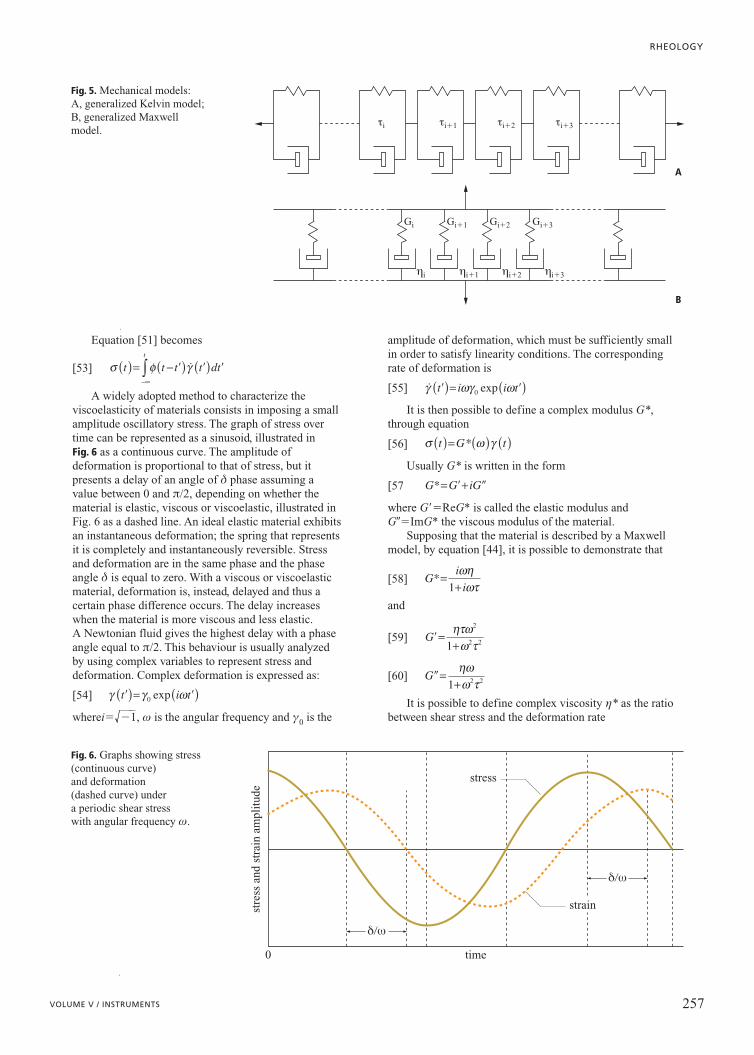
It is possible to conceive models which are morecomplicated than those devised so far, but they can all bereduced to two canonical forms: the generalized Kelvinmodel and the generalized Maxwell model, illustrated in Fig. 5. Alfrey (1945) showed that the two canonical formscan be made mechanically equivalent by suitably choosingthe parameters, and that it is possible to obtain one singlelinear differential equation for one of the two canonicalforms by choice, and vice versa. In other words, viscoelasticbehaviour can be represented in three equivalent ways.
The equation describing the behaviour of a generalizedMaxwell element can be determined by using the linearsuperposition principle. A Maxwell element is described bythe differential equation [44] or in other terms by equation:
[49]
By considering n elements and applying the linearsuperposition principle, one obtains
[50]
where tM and tJ are the parameters of the i-th component.Equation [50] can be extended to include a continuous
distribution of relaxation times
[51]
By introducing then a relaxation function /, defined by:
[52] φ ττ
τ τt tN
t t d−( )= ( ) − −( ) ∞
∫ 0
exp
σ ττ
τ γ τtN
t t t dt dt
( )= ( ) − −( ) ( )∞
−∞∫ ∫0
exp
σ ητ
τ γt t t t dti
ii
t( )= − −( ) ( )−∞∫∑ exp
σ ητ
τ γt t t t dtt( )= − −( ) ( )−∞∫ exp
σ τ τ σ τ τ σ η η γ τ η τ η+ +( ) +( ) = +( ) + +( )3 4 3 4 3 4 4 3 3 4 γ
σ τ σ η γ τ γ+ = +( )M J
σ ηγ τ= −( )exp t M
σ ηγ τ= − −( ) 1 exp t M
σ τ σ ηγ+ =M
γ σ τ=( ) − −( ) G t K1 exp
FLUID MOTION
256 ENCYCLOPAEDIA OF HYDROCARBONS
A B
gn
g
gEsE
s
snG
G
h
h
Fig. 4. Mechanical models: A, Kelvin model; B, Maxwell model.
Equation [51] becomes
[53]
A widely adopted method to characterize theviscoelasticity of materials consists in imposing a smallamplitude oscillatory stress. The graph of stress overtime can be represented as a sinusoid, illustrated in Fig. 6 as a continuous curve. The amplitude ofdeformation is proportional to that of stress, but itpresents a delay of an angle of d phase assuming avalue between 0 and p/2, depending on whether thematerial is elastic, viscous or viscoelastic, illustrated inFig. 6 as a dashed line. An ideal elastic material exhibitsan instantaneous deformation; the spring that representsit is completely and instantaneously reversible. Stressand deformation are in the same phase and the phaseangle d is equal to zero. With a viscous or viscoelasticmaterial, deformation is, instead, delayed and thus acertain phase difference occurs. The delay increaseswhen the material is more viscous and less elastic. A Newtonian fluid gives the highest delay with a phaseangle equal to p/2. This behaviour is usually analyzedby using complex variables to represent stress anddeformation. Complex deformation is expressed as:
[54]
wherei12
1, w is the angular frequency and g0 is the
amplitude of deformation, which must be sufficiently smallin order to satisfy linearity conditions. The correspondingrate of deformation is
[55]
It is then possible to define a complex modulus G*,through equation
[56]
Usually G* is written in the form
[57
where GReG* is called the elastic modulus andGImG* the viscous modulus of the material.
Supposing that the material is described by a Maxwellmodel, by equation [44], it is possible to demonstrate that
[58]
and
[59]
[60]
It is possible to define complex viscosity h* as the ratiobetween shear stress and the deformation rate
G=+ηωω τ1 2 2
G=+ητωω τ
2
2 21
G ii
*=+ωηωτ1
G G iG*= +
σ ω γt G t( )= ( ) ( )*
γ ωγ ωt i i t ( )= ( )0 exp
γ γ ωt i t ( )= ( )0 exp
σ φ γt t t t dtt
( )= −( ) ( )−∞∫
RHEOLOGY
257VOLUME V / INSTRUMENTS
A
B
Gi2
hi2
Gi3
hi3
Gi1
hi1
Gi
ti2 ti3ti ti1
hi
Fig. 5. Mechanical models: A, generalized Kelvin model;B, generalized Maxwellmodel.
strain
stress
time0
stre
ss a
nd s
trai
n am
plit
ude
dw
dw
Fig. 6. Graphs showing stress(continuous curve) and deformation (dashed curve) under a periodic shear stresswith angular frequency w.

[61]
It is therefore possible to write:
[62]
h is usually called dynamic viscosity. There are also
[63]
and
[64]
Often the results of oscillatory tests are presented interms of dynamic viscosity h and elastic modulus G. Fig. 7shows the graph of these two normalized functions for aMaxwell model, as a function of normalized frequency wt.In two decades only, centered across wt1, the graph goesfrom a markedly viscous behaviour (G0), at lowfrequencies, to a markedly elastic one (h0). In this way, itis possible to clearly understand t as the characteristic timeof the Maxwell model.
Linear viscoelastic responses in oscillatory tests can beconveniently represented by reporting the elastic modulus Gand the delay angle d. If the deformation has the formdescribed in equation [54], then stress has a similar form butits phase has a d angle anticipation, and therefore
[65]
It is possible to demonstrate that
[66]
4.3.6 Viscosity of polymeric fluids
The study of polymeric systems assumed great relevance inthe development of rheology. This circumstance is relatedparticularly to the enormous practical importance ofpolymeric fluids, but also to the fact that polymers can beconsidered as model systems. By suitably changing thecharacteristics of their molecular architecture, it is possibleto vary and control their rheological properties. There are
many publications dealing with the rheological behaviour ofpolymers in detail: from Ferry’s book (1980) focusing onaspects related to linear viscoelasticity, to the books of Birdet al. (1987a, b) and Larson (1988) dealing in detail with theproblem of constitutive equations, to the works of Tanner(1985) and of Baird and Dimitris (1995) that discuss thefluxes generated in polymer processing operations.
The generic name polymeric fluids describes verydifferent systems: from scarcely viscous systems, forinstance very diluted polymer solutions, to increasinglyrigid materials obtained by increasing the concentration ofthe solution, up to polymer ‘melts’. In any case, polymericfluids in general often show strong viscoelastic effects,among which pseudoplasticity, normal stresses and time-dependent behaviour. The most relevant factor whichdetermines the rheologic behaviour of polymeric fluids ischain length, apart from the fact that macromolecules caneasily be distorted even when involved in slow fluxes.Another very important factor is the fact that the differentchains can form temporary links, under the effect ofintermolecular forces, or permanent links by crosslinking.When the chains are long enough, they form intermolecularassociations called entanglements, which are responsible forthe elasticity phenomena, such as normal stresses or highextensional viscosities. Entanglements are topologicalconstraints to the molecular motion derived from the factthat macromolecules cannot cross each other. Due to thepresence of entanglements, a macromolecule surrounded byothers is not capable of moving very far in directionsperpendicular to its molecular contour (Edwards, 1967). Forthis reason, diffusion or molecular relaxation are limited toa motion called reptation, similar to the movement of asnake (De Gennes, 1971), which takes place along the tubesurrounding the polymer profile. For this reason, therelaxation of a polymer that forms entanglements is slow,and its viscosity is high. In fact, according to the De Gennesmodel, viscosity should be considered proportional to thetime necessary for a molecule to travel, by diffusing adistance equal to its length within the tube. This time,according to calculations, is proportional to the cube of thepolymer molecular weight Mw.
Entanglements have a very important role indetermining the effect of the polymer molecular weight onthe rheological behaviour of polymer melts, as illustrated inthe logarithmic diagram of Fig. 8, showing viscosity at adeformation rate very close to zero as a function ofmolecular weight (curves are scaled according to a series ofconstant factors). For low molecular weights, viscositygrows like Mw
1.0, whereas above a critical value of molecularweight Mc, viscosity grows like Mw
3.4 and when themolecular weight is equal to Mc a sudden slope variationoccurs. Above a critical point, polymeric melts showmarked elastic properties. The distinct behaviour differenceis due to entanglement formation. Functional dependence ishowever slightly different from that predicted by the DeGennes theory, as the exponent of Mw is slightly above 3. Agreat number of non-Newtonian effects can be explained interms of entanglement density variations. In a polymericmelt, the flow causes a relative movement of polymericchains so that some entanglements disappear, but others cansimultaneously form, as occurs in conditions of rest. In anyflow situation, the entanglement density depends on thedynamic equilibrium between formation and destruction
tanδ =G G
σ σ ω δt i t( )= +( ) 0 exp
G =η ω
G =η ω
η η η*= − i
σ η γt t( )= ( )*
FLUID MOTION
258 ENCYCLOPAEDIA OF HYDROCARBONS
1
0 11log (wt)
GG
GG
hh
Fig. 7. Maxwell model under oscillatory stress: normalized moduli and dynamic viscosity variation as a function of normalized frequency wt (thG).

rates. If the flux is slow, this density tends towards that ofrest conditions, and viscosity tends towards its Newtonianvalue, whereas if the fluid is fast, there is a decrease notonly in this density but also in the difficulty of reciprocallymoving molecules. In this way, it is possible to explainpseudoplastic flow curves with a Newtonian plateau at lowshear rates typical of many polymeric melts. Thedependence of viscosity on the concentration of polymer insolution is also important. Generally, at low values ofconcentration c, viscosity grows proportionally to c. Bygradually increasing the concentration, one enters in aregime where viscosity grows like cn, where n is generallyequal to 3, but it can also assume higher values. Thistransition is still related to the entanglement formation.Once again, by passing from one regime to the other, theelastic properties of the system change.
Another very important system is represented by gels,usually composed of solutions where polymeric chains arecrosslinked by permanent bonds. Typical examples arevulcanized rubbers, but also systems where crystallineregions are bonded by chains passing through them as occursin semicrystalline polymers. Another way of forming a gel isto add significant amounts (with concentrations around 20%in volume) of small solid particles, such as carbon black, to apolymeric melt, so that chains form bridges between them byabsorbing nearby particles. When a precursor fluid, whichmay consist of small molecules or polymers, is crosslinkedto form a gel, its rheological properties vary from those of aviscous liquid to those of an elastic solid, and thus viscositydiverges and becomes infinite, whereas the low frequencymodulus G0 changes from zero to a value equal to
[67]
where n is the number of crosslinking points for volume, k isthe Boltzmann constant and T is temperature.
4.3.7 Rheology of disperse systems
The dispersions of particles in a liquid are extremelycommon systems (for instance blood, paint, ink, cement).Dispersion rheology is another subject to which muchattention was given in recent years (Russel et al., 1989;Brady, 1996; Mellema, 1997). Even the simplest suspensionmodel, made up of rigid spheres interacting only by rigidrepulsions when they come into contact, shows quitecomplex rheological behaviours. At very low volumetricfractions (/0.03), suspension viscosity can be describedby the following equation
[68]
where hs was derived by Albert Einstein (1906) from thecalculation of the viscous dissipation produced by the fluxaround a single sphere. Often rheological data ofdispersions are expressed in terms of relative viscosityhrhhs. Equation [68] is valid only when the suspensionis sufficiently diluted to ensure the flow field around aparticle is not significantly influenced by the presence ofother particles. As the volumetric fraction increases,however, hydrodynamic interactions start becomingsignificant. The effect of two-body interactions generates acontribution to the value of h proportional to /2, calculatedby George Keith Batchelor (1971), who derived thefollowing expression
[69]
Equation [69] can be extended to higher powers of /, byadopting a method that uses the concept of effectivemedium. Consider an increase of the volumetric fraction ofparticles of an infinitesimal quantity d/ in a suspension withh(/) viscosity. By treating this suspension to which particlesare added as if it were a homogeneous viscous medium withh(/) viscosity, the increase in viscosity caused by particleaddition can be calculated by using Eq. [68], thus
[70]
which when integrated gives:
[71] η η φ= ( )s exp 5 2
d dη η φ φ= ( )2 5.
η η φ φ= + +( )s 1 2 5 6 2 2. .
η η φ= +( )s 1 2 5.
G kT0 =ν
RHEOLOGY
259VOLUME V / INSTRUMENTS
polydimethylsiloxane
polybutadiene
polymethylmethacrylate
polystyrene
1
2
3
4
1.0
60 1 2 3 4 5
log
h
con
st.
log Mw const.
1
2
3
4
Fig. 8. Relationship between low shear viscosity and the polymer molecular weight for a series of monodispersed polymer melts; curves scaled according to constant factors on the x and y axes (Ferry, 1980).

This relationship does not take correlations betweenspheres into account due to their finite dimensions. In otherwords, due to packing problems, a particle requires greaterspace than its volume when added to a relativelyconcentrated dispersion. For this reason, instead of d/, it isnecessary to use d/(1K/), where K accounts for thesecrowding effects. Therefore
[72]
This equation demonstrates that viscosity becomesinfinite when /1K, and thus 1K can be identified withthe maximum packing fraction /m. Observe
[73]
which is valid for spherical particle suspensions, but can beextended to any form becoming
[74]
where the intrinsic viscosity [h] of the suspension isintroduced, defined as
[75]
Equation [74] was formulated and named after Kriegerand Dougherty in 1959. The value of /m strongly depends onparticle size distribution, and it increases as polydispersityincreases. For a monodispersed rigid sphere system, it is/m0.63-0.64. Generally rigid sphere dispersions behavelike Newtonian fluids up to volumetric fractions / in theorder of 0.3, but for higher values viscosity starts dependingon the shear rate. This dependency is due to the fact that theshear rate disturbs the distribution of particle positions withrespect to equilibrium. The velocity at which the equilibriumsituation is recovered is controlled by particle diffusivity,which in diluted solutions is equal to
[76]
where a is the particle radius.The time tD needed for a particle to diffuse for a distance
equal to its radius a is therefore given by
[77]
It is possible to define an adimensional rate ofdeformation Pe, called the Péclet number, as follows:
[78]
Krieger (1972) suggested expressing rheological data forsuspensions in terms of the reduced stress sr
[79]
The relative viscosity of concentrated dispersions shouldtherefore be a universal function of two adimensionalquantities, / and sr. This function can be expressed by thefollowing relationship:
[80]
where hr0is the low shear relative viscosity, hr
is the highshear relative viscosity and b is a fitting parameter. The
difference at high sr values is due to the dilatancyphenomena.
As already seen, the dependency of hr0on / follows the
Krieger-Dougherty equation [74], but it can also be observedthat the dependency of hr
can be described by the sameequation, as long as a higher value of /m is used. This resultcan be associated with the fact that at high sheardeformation rates, particles tend to find more favorablegeometrical positions, which permit better packing, such asbidimensional structures, for instance.
Moreover, it was observed that concentrated dispersions(/0,40) exhibit dilatancy phenomena at high shear rates,higher than the rates at which pseudoplasticity usuallyappears. The bidimensional structures just mentionedjustifying pseudoplastic effects, are unstable and aredestroyed at a certain critical shear rate, creating a randomarrangement that causes a viscosity increase. It wasdemonstrated that this critical value varies little when thevolumetric fraction of particles is in the order of 0.50, but itdecreases markedly when / is significantly higher than 0.50.
In rigid sphere suspensions, viscous characteristics arestrongly dominate over elastic ones, but, nevertheless, theelastic modulus G is not zero. This weak elasticity isproduced by Brownian motion that tends to establishequilibrium when particle configuration is distorted by ashear action. However G consistently increases whenparticle concentration increases, since characteristic times ofrelaxation of suspensions decrease as particle diffusivitydecreases at high concentrations.
Often, in addition to particles in a dispersed system, othertypes of interactions, besides hydrodynamic, are present,generating a potential barrier kinetically hindering particlecoagulation. This can be obtained by adsorbing a polymerlayer on the particle surface. When two adsorbed layersoverlap, a repulsive force arises if the compression ofpolymer molecules is favored with respect to their mixing. Inorder to account for the adsorbed layer in describing therheological behaviour of dispersions, it is necessary to correctthe volumetric fraction by introducing an effective value
[81]
where d represents the layer width. Another common way tostabilize suspensions is to electrostatically charge particlesurfaces, and this is often obtained by adsorbing ionicsurfactants which create a double electric layer around theparticles, themselves. Since consequential electrostaticaction keeps particles apart, its effect is to increase theeffective value of their diameter; there are several equationsfor calculating deff from the interaction potential, from whichit is then possible to derive:
[82]
The enlargement of the effective diameter influences lowshear viscosity in electrostatically stabilized dispersions.Russel (1978) derived an expression as a development up tothe second order of / for a disordered suspension of chargedspheres
[83]ηη
φ φs
effda
= + + +
1 2 5 2 53
40
5
2. .
φ φeffeffda
=
2
3
φ φ δeff a= +
1
3
η ηη η
σr rr r
rb= +
−+
∞
∞0
1
σ σr
akT
≡3
Pe akT
tsD≡ ∝η γ γ
3
t aD
akTD
s≈ =2
0
36πη
D kTas
0 6=πη
η η ηφηφ
[ ]= −→
lim0
s
s
η η φ φ η φ= −( )−[ ]s mm1
η η φ φφ
= −( )−s mm
15 2( / )
η η φ= −( )−sKK1 5 2
FLUID MOTION
260 ENCYCLOPAEDIA OF HYDROCARBONS
The presence of a surface electrostatic charge has amuch stronger effect on the /2 coefficient with respect to therigid sphere case. This expression is valid only for values of/ of around 0.10, whereas for higher concentrations, it isconvenient to extend the Krieger-Dougherty equation [74]
[84]
As the deformation rate increases, the hydrodynamiccontribution to viscosity increases with respect to theelectrostatic one, causing pseudoplastic effects that can beaccounted for by introducing a dependency of deff on the rateof deformation, so that deff represents an interparticledistance at which the electrostatic and hydrodynamic forcesbalance off. Electrostatically stabilized dispersions can alsopresent a yield stress, when repulsions among particles arehigh enough to create a macrocrystallization phenomena(Larson, 1999).
Bibliography
Choi G.N., Krieger I.M. (1986) Rheological studies on stericallystabilized model dispersions of uniform colloidal spheres. II:Steady-shear viscosity, «Journal of Colloid Interface Science»,113, 101-113.
Papir Y.S., Krieger I.M. (1970) Rheological studies on dispersionsof uniform colloidal spheres. II: Dispersions in nonaqueous media,«Journal of Colloid Interface Science», 34, 126-130.
Vinogradov G.V., Malkin A.Y. (1980) Rheology of polymers,Moscow, Mir; Berlin, Springer.
References
Alfrey T. Jr. (1945) Methods of representing the properties ofviscoelastic materials, «Quarterly of Applied Mathematics», 3,143-150.
Baird D.G., Dimitris I.C. (1995) Polymer processing. Principles anddesign, Boston (MA)-Oxford, Butterworths.
Barnes H.A. (1997) Thixotropy. A review, «Journal of Non-NewtonianFluid Mechanics», 70, 1-33.
Barnes H.A., Walters K. (1985) The yield stress myth, «RheologicaActa», 24, 323-326.
Barnes H.A. et al. (1989) Introduction to rheology, Amsterdam,Elsevier.
Batchelor G. K. (1971) The stress generated in a non-dilute suspensionof elongated particles in pure straining motion, «Journal of FluidMechanics», 46, 813-829.
Bird R.B. et al. (1987a) The dynamics of polymeric liquids, New York,John Wiley, 2v.; v.I: Fluid mechanics.
Bird R.B. et al. (1987b) The dynamics of polymeric liquids, New York,John Wiley, 2v.; v.II: Kinetic theory.
Brady J.F. (1996) Model hard-sphere dispersions: statistical mechanicaltheory, simulations, and experiments, «Current Opinion in Colloidand Interface Science», 1, 472-480.
Carreau P.J. (1972) Rheological equations from molecular networkstheories, «Transactions of the Society of Rheology», 16, 99-127.
Cross M.M. (1965) Rheology of non-newtonian fluids: a new flowequation for pseudo-plastic systems, «Journal of Colloidal Science»,20, 417-437.
De Gennes P.G. (1971) Reptation of a polymer chain in the presenceof fixed obstacles, «Journal of Chemical Physics», 55, 572-579.
Edwards S.F. (1967) The statistical mechanics of polymerized material,«Proceedings of the Physical Society», 92, 9-16.
Einstein A. (1906) Eine neue Bestimmung der Molekuldimension,«Annalen der Physik», 19, 289-306.
Ferry J.D. (1980) Viscoelastic properties of polymers, New York, JohnWiley.
Hooke R. (1931) Lectures de potentia restitutiva, Oxford, OxfordUniversity Press.
Jones D.M. et al. (1987) On the extensional viscosity of mobile polymersolutions, «Rheologica Acta», 26, 20-30.
Krieger I.M. (1972) Rheology of monodispersed latices, «Advancesin Colloid and Interface Science», 3, 111-136.
Krieger I.M., Dougherty T.J. (1959) A mechanism for non-newtonianflow in suspensions of rigid spheres, «Transactions of the Societyof Rheology», 3, 137-152.
Krieger I.M., Maron S.H. (1954) Direct determination of the flowcurves of non-newtonian fluids. III: Standardized treatment ofviscometric data, «Journal of Applied Physics», 25, 72-75.
Larson R.G. (1988) Constitutive equations for polymer melts andsolutions, Boston (MA)-London, Butterworths.
Larson R.G. (1999) The structure and properties of complex fluids,New York-Oxford, Oxford University Press.
Mellema J. (1997) Experimental rheology of model colloidaldispersions, «Current Opinion in Colloid and Interface Science»,2, 411-419.
Newton I. (1999) The Principia. Mathematical principles of naturalphilosophy, Berkeley (CA), University of California Press.
Reiner M. (1964) The Deborah number, «Physics Today», January,62.
Russel W.B. (1978) The rheology of suspensions of charged rigidspheres, «Journal of Fluid Mechanics», 85, 209-232.
Russel W.B. et al. (1989) Colloidal dispersions, Cambridge, CambridgeUniversity Press.
Sisko A.W. (1958) The flow of lubricating greases, «Industrial andEngineering Chemistry», 50, 1789-1792.
Tanner R.I. (1985) Engineering rheology, Oxford, Clarendon Press.
Walters K. (1975) Rheometry, London, Chapman & Hall.
Stefano Carrà
MAPEI
Milano, Italy
ηη
φφ
φ
s
eff
m
m
= −
−( )
15 2
RHEOLOGY
261VOLUME V / INSTRUMENTS