4434 IEEE SENSORS JOURNAL, VOL. 14, NO. 12, DECEMBER 2014

Mapping Tree Species in Coastal Portugal UsingStatistically Segmented Principal Component

Analysis and Other MethodsPrem Chandra Pandey, Member, IEEE, Nicholas J. Tate, and Heiko Balzter

Abstract— Hyperspectral sensors record radiances in a largenumber of wavelengths of the electromagnetic spectrum and canbe used to distinguish different tree species based on their charac-teristic reflectance signatures. Reflectance spectra were measuredfrom airborne hyperspectral AISA Eagle/Hawk imagery in orderto identify different Mediterranean tree species at a coastaltest site in Portugal. A spectral range from 400 to 2450 nmwas recorded at 2-m spatial resolution. The hyperspectral dataare divided into five spectral data ranges. The chosen rangesfor segmentation are based on statistical properties as well ason their wavelengths, as radiances of a particular wavelengthmay overlap with neighboring wavelengths. Principal componentanalysis (PCA) is applied individually to each spectral range.The first three principal components (PCs) of each range arechosen and are fused into a new data segment of reduceddimensionality. The resulting 15 PCs contain 99.42% of theinformation content of the original hyperspectral image. ThesePCs were used for a maximum likelihood classification (MLC).Spectral signatures were also analyzed for the hyperspectraldata, and were validated with ground data collected in the fieldby a handheld spectro-radiometer. Different RGB combinationsof PC bands of segmented PC image provide distinct featureidentification. A comparison with other classification approaches(spectral angle mapper and MLC of the original hyperspectralimagery) shows that the MLC of the segmented PCA achievesthe highest accuracy, due to its ability to reduce the Hughesphenomenon.

Index Terms— Hyperspectral remote sensing, segmented prin-cipal component analysis, maximum likelihood classification,spectral angle mapper, forest mapping, ground data, coastalvegetation.

I. INTRODUCTION

HYPERSPECTRAL images provide the potential for moreaccurate and detailed spectral information extraction

compared to other types of remotely sensed data, due to theirlarge number of spectral bands. Researchers have successfully

Manuscript received May 15, 2014; revised June 23, 2014; acceptedJune 24, 2014. Date of publication July 8, 2014; date of current ver-sion October 23, 2014. The work of P. C. Pandey was supported bythe Association of Commonwealth Universities (INCS-2011-155 Com-monwealth Fellowship). The work of H. Balzter was supported bythe Royal Society Wolfson Research Merit Award, 2011/R3. The associateeditor coordinating the review of this paper and approving it for publicationwas Prof. Octavian Postolache.

P. C. Pandey and H. Balzter are with the Centre for Landscape andClimate Research, Department of Geography, University of Leicester,Leicester LE1 7RH, U.K. (e-mail: prem26bit@gmail.com; pcp6@le.ac.uk;hb91@le.ac.uk).

N. J. Tate is with the Department of Geography, University of Leicester,Leicester LE1 7RH, U.K. (e-mail: njt9@le.ac.uk).

Color versions of one or more of the figures in this paper are availableonline at http://ieeexplore.ieee.org.

Digital Object Identifier 10.1109/JSEN.2014.2335612

used hyperspectral imagery to map vegetation species [1],invasive species [2], above-ground biomass [3], environmentalparameters [4] and vegetation stress and disease [5]. Previousstudies show that multi-sensor approaches have been usedto discriminate tree species for forest management usingtechniques such as spectral reflectance [6], Support VectorMachines (SVM) [7], MLC and SAM [8]. Over the pastdecades, different classification techniques have been devel-oped for hyperspectral data [9]. They were compared forapplications to land use / land cover mapping and otherremote sensing purposes and MLC has been considered assuperior to other classifier approaches [10]–[12]. MLC isbased on the class probability density functions assuminga multivariate normal distribution and often achieves moreaccurate results than other methods [13]. MLC is availablein most software packages like ENVI©, Arc GIS�, ERDASImagine� [14], [15].

The high spectral resolution and large number of spectralbands of hyperspectral images enable a better identification ofland use / land cover types [16], [17] as well as other featureslike vegetation type, crop type and soils [15], [18]. Hyper-spectral imaging enables an effective mapping of vegetationin diverse environments like estuaries [19], marshland [20]and tropical rainforest [21]. However, the high data volumeand dimensionality of hyperspectral data is a constraint forinformation extraction due to long processing times [22].This needs to be resolved using compression techniques toreduce the dimensionality of the data while retaining enoughof the original spectral information [22]–[24]. In digital imageprocessing, PCA is commonly used for image compression.It performs a multidimensional coordinate system rotationto convert the original inter-correlated bands into a new setof uncorrelated PCs where a small number of PCs containsmost of the variation. Karathanassi [25] described PCA as amathematically rigorous technique where the original spectralinformation is retained. Segmented PCA was developed toreduce the ‘Hughes phenomenon’, which means that by addingmore spectral bands to a standard MLC the classificationresult eventually becomes less accurate [22], [26]. Too manyinput bands can thus lead to a degradation of the classifiedmap. Bellman [27] investigated the relationship between thenumber of bands and the number of training samples forimage classification and termed it the ‘curse of dimension-ality’ due to the rapid increase in required training samplesfor density estimation. As dimensionality increases with thenumber of bands, the number of training samples needed for

1530-437X © 2014 IEEE. Translations and content mining are permitted for academic research only. Personal use is also permitted, butrepublication/redistribution requires IEEE permission. See http://www.ieee.org/publications_standards/publications/rights/index.html for more information.

PANDEY et al.: MAPPING TREE SPECIES IN COASTAL PORTUGAL 4435

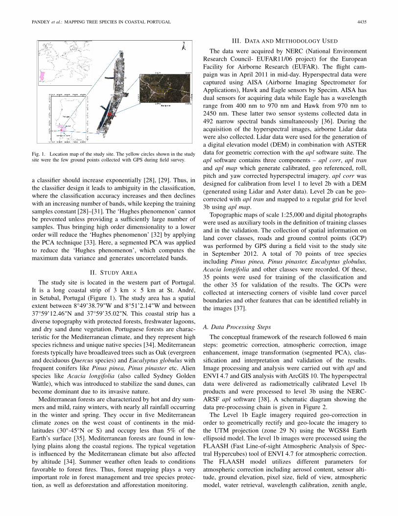
Fig. 1. Location map of the study site. The yellow circles shown in the studysite were the few ground points collected with GPS during field survey.

a classifier should increase exponentially [28], [29]. Thus, inthe classifier design it leads to ambiguity in the classification,where the classification accuracy increases and then declineswith an increasing number of bands, while keeping the trainingsamples constant [28]–[31]. The ‘Hughes phenomenon’ cannotbe prevented unless providing a sufficiently large number ofsamples. Thus bringing high order dimensionality to a lowerorder will reduce the ‘Hughes phenomenon’ [32] by applyingthe PCA technique [33]. Here, a segmented PCA was appliedto reduce the ‘Hughes phenomenon’, which computes themaximum data variance and generates uncorrelated bands.

II. STUDY AREA

The study site is located in the western part of Portugal.It is a long coastal strip of 3 km × 5 km at St. André,in Setubal, Portugal (Figure 1). The study area has a spatialextent between 8°49’38.79"W and 8°51’2.14"W and between37°59’12.46"N and 37°59’35.02"N. This coastal strip has adiverse topography with protected forests, freshwater lagoons,and dry sand dune vegetation. Portuguese forests are charac-teristic for the Mediterranean climate, and they represent highspecies richness and unique native species [34]. Mediterraneanforests typically have broadleaved trees such as Oak (evergreenand deciduous Quercus species) and Eucalyptus globulus withfrequent conifers like Pinus pinea, Pinus pinaster etc. Alienspecies like Acacia longifolia (also called Sydney GoldenWattle), which was introduced to stabilize the sand dunes, canbecome dominant due to its invasive nature.

Mediterranean forests are characterized by hot and dry sum-mers and mild, rainy winters, with nearly all rainfall occurringin the winter and spring. They occur in five Mediterraneanclimate zones on the west coast of continents in the mid-latitudes (30°-45°N or S) and occupy less than 5% of theEarth’s surface [35]. Mediterranean forests are found in low-lying plains along the coastal regions. The typical vegetationis influenced by the Mediterranean climate but also affectedby altitude [34]. Summer weather often leads to conditionsfavorable to forest fires. Thus, forest mapping plays a veryimportant role in forest management and tree species protec-tion, as well as deforestation and afforestation monitoring.

III. DATA AND METHODOLOGY USED

The data were acquired by NERC (National EnvironmentResearch Council- EUFAR11/06 project) for the EuropeanFacility for Airborne Research (EUFAR). The flight cam-paign was in April 2011 in mid-day. Hyperspectral data werecaptured using AISA (Airborne Imaging Spectrometer forApplications), Hawk and Eagle sensors by Specim. AISA hasdual sensors for acquiring data while Eagle has a wavelengthrange from 400 nm to 970 nm and Hawk from 970 nm to2450 nm. These latter two sensor systems collected data in492 narrow spectral bands simultaneously [36]. During theacquisition of the hyperspectral images, airborne Lidar datawere also collected. Lidar data were used for the generation ofa digital elevation model (DEM) in combination with ASTERdata for geometric correction with the apl software suite. Theapl software contains three components – apl corr, apl tranand apl map which generate calibrated, geo referenced, roll,pitch and yaw corrected hyperspectral imagery. apl corr wasdesigned for calibration from level 1 to level 2b with a DEM(generated using Lidar and Aster data). Level 2b can be geo-corrected with apl tran and mapped to a regular grid for level3b using apl map.

Topographic maps of scale 1:25,000 and digital photographswere used as auxiliary tools in the definition of training classesand in the validation. The collection of spatial information onland cover classes, roads and ground control points (GCP)was performed by GPS during a field visit to the study sitein September 2012. A total of 70 points of tree speciesincluding Pinus pinea, Pinus pinaster, Eucalyptus globulus,Acacia longifolia and other classes were recorded. Of these,35 points were used for training of the classification andthe other 35 for validation of the results. The GCPs werecollected at intersecting corners of visible land cover parcelboundaries and other features that can be identified reliably inthe images [37].

A. Data Processing Steps

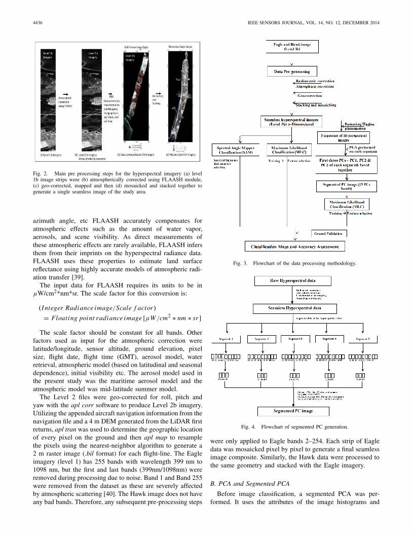
The conceptual framework of the research followed 6 mainsteps: geometric correction, atmospheric correction, imageenhancement, image transformation (segmented PCA), clas-sification and interpretation and validation of the results.Image processing and analysis were carried out with apl andENVI 4.7 and GIS analysis with ArcGIS 10. The hyperspectraldata were delivered as radiometrically calibrated Level 1bproducts and were processed to level 3b using the NERC-ARSF apl software [38]. A schematic diagram showing thedata pre-processing chain is given in Figure 2.

The Level 1b Eagle imagery required geo-correction inorder to geometrically rectify and geo-locate the imagery tothe UTM projection (zone 29 N) using the WGS84 Earthellipsoid model. The level 1b images were processed using theFLAASH (Fast Line-of-sight Atmospheric Analysis of Spec-tral Hypercubes) tool of ENVI 4.7 for atmospheric correction.The FLAASH model utilizes different parameters foratmospheric correction including aerosol content, sensor alti-tude, ground elevation, pixel size, field of view, atmosphericmodel, water retrieval, wavelength calibration, zenith angle,

4436 IEEE SENSORS JOURNAL, VOL. 14, NO. 12, DECEMBER 2014

Fig. 2. Main pre processing steps for the hyperspectral imagery (a) level1b image strips were (b) atmospherically corrected using FLAASH module,(c) geo-corrected, mapped and then (d) mosaicked and stacked together togenerate a single seamless image of the study area.

azimuth angle, etc FLAASH accurately compensates foratmospheric effects such as the amount of water vapor,aerosols, and scene visibility. As direct measurements ofthese atmospheric effects are rarely available, FLAASH infersthem from their imprints on the hyperspectral radiance data.FLAASH uses these properties to estimate land surfacereflectance using highly accurate models of atmospheric radi-ation transfer [39].

The input data for FLAASH requires its units to be inμW/cm2*nm*sr. The scale factor for this conversion is:

(Integer Radiance image/Scale f actor)

= Floating point radiance image [μW/cm2 ∗ nm ∗ sr ]The scale factor should be constant for all bands. Other

factors used as input for the atmospheric correction werelatitude/longitude, sensor altitude, ground elevation, pixelsize, flight date, flight time (GMT), aerosol model, waterretrieval, atmospheric model (based on latitudinal and seasonaldependence), initial visibility etc. The aerosol model used inthe present study was the maritime aerosol model and theatmospheric model was mid-latitude summer model.

The Level 2 files were geo-corrected for roll, pitch andyaw with the apl corr software to produce Level 2b imagery.Utilizing the appended aircraft navigation information from thenavigation file and a 4 m DEM generated from the LiDAR firstreturns, apl tran was used to determine the geographic locationof every pixel on the ground and then apl map to resamplethe pixels using the nearest-neighbor algorithm to generate a2 m raster image (.bil format) for each flight-line. The Eagleimagery (level 1) has 255 bands with wavelength 399 nm to1098 nm, but the first and last bands (399nm/1098nm) wereremoved during processing due to noise. Band 1 and Band 255were removed from the dataset as these are severely affectedby atmospheric scattering [40]. The Hawk image does not haveany bad bands. Therefore, any subsequent pre-processing steps

Fig. 3. Flowchart of the data processing methodology.

Fig. 4. Flowchart of segmented PC generation.

were only applied to Eagle bands 2–254. Each strip of Eagledata was mosaicked pixel by pixel to generate a final seamlessimage composite. Similarly, the Hawk data were processed tothe same geometry and stacked with the Eagle imagery.

B. PCA and Segmented PCA

Before image classification, a segmented PCA was per-formed. It uses the attributes of the image histograms and

PANDEY et al.: MAPPING TREE SPECIES IN COASTAL PORTUGAL 4437

Fig. 5. Different red, blue, green channel combinations of the 15 fused segmented PCs (for A1, A2, A3, B1 etc. refer to Table I).

TABLE I

SEGMENTATION OF HYPERSPECTRAL DATA FROM PCA WITHIN FIVE SPECTRAL DATA SEGMENTS

wavelengths as illustrated in Figure 4. The segmented PCAapproach is utilized to calculate a dataset of reduced dimen-sionality as input for the maximum likelihood classifier. Inorder to increase the classification performance, the segmentedPCA technique is used to remove redundant bands withoutlosing significant information. A PCA was applied to the 5different segments of the hyperspectral bands. The first 3 PCsof each of the 5 segments were combined to generate an imagewith 15 PC bands as shown in Figure 5. The 15 segmentedPC bands contain most of the variability of the original253 Eagle bands and 256 Hawk bands. Thus, almost all ofthe hyperspectral information is retained and band redundancyand data volume are reduced.

The different PCs are shown in Figure 5 as RGB channelcombinations which clearly show the retention of the spectralinformation as well as visually distinct feature classes. Thespectrally segmented PCA results for the 5 different spectralsegments are shown in Table I. The higher orders PCs werediscarded because they contain mostly noise (eigenvalue < 1).By combining the first 3 PCs from each of the 5 segmenteddatasets, 15 PC bands contain most of the spectral information

TABLE II

EIGENVALUES FOR THE FIRST THREE PCS DERIVED FROM THE

SEGMENTED PCA OF THE HYPERSPECTRAL IMAGE

of the original hyperspectral data (Figure 4). In the segmentedPCA, the hyperspectral bands are subdivided into spectralsegments based on band histogram statistics and wavelengthsas shown in Table I. On each segment of hyperspectral databands, a PCA is performed to generate the same number ofPCs as the number of input bands (Table I and Figure 4). Thefirst 3 PCs with the highest eigenvalues within each segment(A1, A2, A3, B1, B2, B3…) are fused together to generate thesegmented PC datasets. The first 3 PCs were chosen from eachsegment and fused together to generate the segmented PCsdataset which represent 99.42% of the information content.Different RGB combinations of the segmented PCs are shown

4438 IEEE SENSORS JOURNAL, VOL. 14, NO. 12, DECEMBER 2014

TABLE III

OVERALL ACCURACY AND KAPPA COEFFICIENT FOR MLC, SAM FOR HYPERSPECTRAL IMAGE AND

MLC OBTAINED FOR THE CLASSIFIED SEGMENTED PCA IMAGES

Fig. 6. Classification maps generated using three different classifiertechniques. (a) Spectral angle mapper. (b) Maximum likelihood classi-fier performed on hyperspectral image. (c) Maximum likelihood classifierperformed on segmented fused PCs.

in Figure 5, which clearly enhances the visual interpretationand distinguishes different features. Thereafter, MLC wasapplied to the 15 segmented PCs. A schematic flowchart ofthe methodology is shown in Figure 3.

C. Classification Steps

Two classification approaches (Maximum Likelihood clas-sification [41] and Spectral Angle Mapper [42]) were appliedto have a baseline comparison for the segmented PCA results.The original mosaicked hyperspectral Eagle and Hawk imageswere used in the MLC approach. With the aid of trainingsamples, a supervised MLC was performed. In addition, thespectral signatures and a priori knowledge of tree speciesanother classified map was produced using SAM.

Fig. 7. Graph showing the classification accuracy of the SAM, MLC, andMLC on segmented PCA.

IV. RESULTS

The classification results for the hyperspectral dataset areshown in Figure 6. The statistical accuracy analysis results ofthe classifications are given in Table III and Figure 6. Theoverall accuracy of the MLC of the segmented PC images issignificantly higher than for the SAM and MLC approachesapplied to the hyperspectral data (Table III). The SAM clas-sification is reliant on spectral image characteristics whichcan be influenced by the ‘Hughes phenomenon’ for high-dimensional data. The MLC performed on the segmentedPCA bands reduces the ‘Hughes phenomenon’. The MLC andSAM classification accuracies for the datasets are presentedin Table II. User’s and producer’s accuracy for differenttree species and feature classes were presented in Figure 7.

PANDEY et al.: MAPPING TREE SPECIES IN COASTAL PORTUGAL 4439

The accuracy of the MLC based on the segmented PCA is96.38%, which is much higher than for the MLC classificationof the original hyperspectral data (89.67%) and SAM (67.5%).The κ coefficient confirms the superior performance of theMLC on the segmented PC image over the SAM and MLCclassifications of the hyperspectral data. The κ coefficient forthe three classification approaches gives the same order ofclassification performance of the three classifier techniques(Table III). The results of the 3 different classification tech-niques are shown in Figure 6, Figure 7 and Table III.

The PCs of the segmented PC image were uncorrelatedcontaining more than 99% of the information of the originalhyperspectral image. Different PC combinations of the seg-mented PC image were used for visual display using threebands displayed as the red, green and blue channels (RGBchannels in Figure 5). The various RGB combinations ofthe segmented PC images provide visual distinctions betweenland cover and forest types and other features. This processenhances the color contrast by providing visual clarity forimage interpretation, thus helping in selecting the training sam-ples used during classification. These distinctive features in theRGB images were not visible in different band combinationsof the original hyperspectral images.

V. DISCUSSION AND CONCLUSION

Tree species classification from hyperspectral imagery is oflimited accuracy if the data dimensionality is not reduced,because the ‘Hughes phenomenon’ leads to a loss of accuracyif too many bands are added. This study explores the clas-sification accuracy achievable from hyperspectral data usingthe segmented PCA approach. It compares this approach tothe SAM and MLC methods of the original hyperspectraldata. The classification accuracy and κ coefficient are muchhigher for the segmented PCA (>96%; κ = 0.95) than for theother methods when validated with ground control points. Theconclusions from this study are:

• Segmented PCA based on data normalization usinghistogram attributes reduces the dimensionality of thehyperspectral imagery while increasing the classificationaccuracy.

• The MLC of the segmented PCA produces much moreaccurate tree species maps than the MLC and SAMclassifiers.

• 15 bands of the first 3 PCs of the 5 segments from thefull hyperspectral dataset contained >99% of the originalspectral variance.

• Compression techniques like segmented PCA to reducethe hyperspectral image dimensionality lead to muchimproved information content by reducing redundancy ofvery similar spectral bands.

Some authors have shown conventional parametric classifi-cation approaches, i.e. MLC as being limited in their abilityto classify high dimensionality data [43], [44]. Although thismakes MLC unsuitable for raw hyperspectral data, this studyshows that MLC can be used after reducing the dimensionsof the hyperspectral imagery. The segmented PCA methodenhances the contrast of the imagery and provides better visualclarity for image interpretation, thus helping in selecting the

training samples used during MLC. Thus, it provides bettertraining samples and better accuracy [10]–[12]. MLC waschosen in the present study as a classifier after reducing thedimensionality of the hyperspectral data using the segmentedPCA approach.

Finally, the segmented PCA approach used in the presentstudy will be helpful for hyperspectral analysis by reducingthe multidimensional data to smaller dimensionality for imageprocessing while retaining most of the information. This imagecompression technique can be used with other classifica-tion algorithms to achieve accurate tree species identificationresults by reducing data dimensionality and data volume. Thisclassification approach can be used for other applications likeurban mapping, land cover mapping, plant stress detection dueto its visual enhancement, fire scar mapping etc.

ACKNOWLEDGMENT

The authors would like to thank André Große-Stoltenberg,Tillmann Buttschardt (University of Münster, Germany) andKaturah Z. Smithson staff University of Leicester for theirhelp during field work. We would like to extend our sin-cere gratitude to the Airborne Research and Survey Facility(ARSF, Gloucester, U.K.) and Natural Environment ResearchCouncil (NERC) for acquiring airborne data under EUFARproject EUFAR11/06 in 2011. The data were provided byAndré Große-Stoltenberg. P.C. Pandey was supported by theAssociation of Commonwealth Universities, (INCS-2011-155commonwealth fellowship). H. Balzter was supported by theRoyal Society Wolfson Research Merit Award, 2011/R3. Theauthors would like to thank Mark Warren and Emma Carolan(Plymouth Marine Laboratory, Plymouth) for their help inhyperspectral data processing.

REFERENCES

[1] M. A. Cochrane, “Using vegetation reflectance variability for specieslevel classification of hyperspectral data,” Int. J. Remote Sens., vol. 21,no. 10, pp. 2075–2087, Jul. 2000.

[2] G. P. Asner et al., “Invasive species detection in Hawaiian rainforestsusing airborne imaging spectroscopy and LiDAR,” Remote Sens. Envi-ron., vol. 112, no. 5, pp. 1942–1955, May 2008.

[3] Z. Hao, H. Hao, Y. Xu-Guo, Z. Ke-Feng, and G. Yi, “Estimation ofabove-ground biomass using HJ-1 hyperspectral images in HangzhouBay, China,” in Proc. Int. Conf. Inf. Eng. Comput. Sci. (ICIECS),Dec. 2009, pp. 1–4.

[4] H. Cetin, “Comparison of spaceborne and airborne hyperspectral imag-ing systems for environmental mapping,” in Proc. 20th ISPRS Congr.,Tech. Commission VII, Istanbul, Turkey, 2004, pp. 1306–1313.

[5] Y. Kim, D. M. Glenn, J. Park, H. K. Ngugi, and B. L. Lehman,“Hyperspectral image analysis for plant stress detection,” in Proc. Annu.Int. Meeting Amer. Soc. Agricult. Biolo. Eng. (ASABE), Pittsburgh, PA,USA, 2010, pp. 1–11.

[6] P. Kumar, L. K. Sharma, P. C. Pandey, S. Sinha, and M. S. Nathawat,“Geospatial strategy for tropical forest-wildlife reserve biomass estima-tion,” IEEE J. Sel. Topics Appl. Earth Observat. Remote Sens., vol. 6,no. 2, pp. 917–923, Apr. 2013.

[7] S. K. Singh, P. K. Srivastava, M. Gupta, J. K. Thakur, andS. Mukherjee, “Appraisal of land use/land cover of mangrove forestecosystem using support vector machine,” Environ. Earth Sci., vol. 71,no. 5, pp. 2245–2255, Mar. 2014.

[8] M. Frank, P. Zhihong, B. Raber, and C. Lenart, “Vegetation managementof utility corridors using high-resolution hyperspectral imaging andLiDAR,” in Proc. 2nd Workshop Hyperspectral Image Signal Process.Evol. Remote Sens. (WHISPERS), Jun. 2010, pp. 1–4.

[9] M. Schaepman, S. Ustin, A. Plaza, T. Painter, J. Verrelst, and S. Liang,“Earth system science related imaging spectroscopy—An assessment,”Remote Sens. Environ., vol. 113, pp. S123–S137, Sep. 2009.

4440 IEEE SENSORS JOURNAL, VOL. 14, NO. 12, DECEMBER 2014

[10] N. Baatuuwie and L. Van Leeuwen, “Evaluation of three classifiers inmapping forest stand types using medium resolution imagery: A casestudy in the Offinso Forest District, Ghana,” African J. Environ. Sci.Technol., vol. 5, no. 1, pp. 25–36, Jan. 2011.

[11] E. L. Hunter and C. H. Power, “An assessment of two classifica-tion methods for mapping Thames Estuary intertidal habitats usingCASI data,” Int. J. Remote Sens., vol. 23, no. 15 pp. 2989–3008,Nov. 2002.

[12] H. Z. M. Shafri, A. Suhaili, and S. Mansor, “The performance of max-imum likelihood, spectral angle mapper, neural network and decisiontree classifiers in hyperspectral image analysis,” J. Comput. Sci., vol. 3,no. 6, p. 419, Jun. 2007.

[13] P. M. Mather, B. Tso, and M. Koch, “An evaluation of Landsat TMspectral data and SAR-derived textural information for lithologicaldiscrimination in the Red Sea Hills, Sudan,” Int. J. Remote Sens., vol. 19,no. 4, pp. 587–604, Mar. 1998.

[14] A. O. Onojeghuo and G. A. Blackburn, “Mapping reedbed habitats usingtexture-based classification of QuickBird imagery,” Int. J. Remote Sens.,vol. 32, no. 23, pp. 8121–8138, Sep. 2011.

[15] A. O. Onojeghuo and G. A. Blackburn, “Optimising the use of hyper-spectral and LiDAR data for mapping reedbed habitats,” Remote Sens.Environ., vol. 115, no. 8, pp. 2025–2034, Aug. 2011.

[16] K. Jusoff, “Land use and cover mapping with airborne hyperspectralimager in Setiu, Malaysia,” J. Agricult. Sci., vol. 1, no. 2, pp. 120–131,2009.

[17] G. P. Petropoulos, K. Arvanitis, and N. Sigrimis, “Hyperion hyperspec-tral imagery analysis combined with machine learning classifiers for landuse/cover mapping,” Expert Syst. Appl., vol. 39, no. 3, pp. 3800–3809,Feb. 2012.

[18] P. Gong, R. Pu, and J. R. Miller, “Correlating leaf area index ofponderosa pine with hyperspectral CASI data,” Can. J. Remote Sens.,vol. 18, pp. 275–282, Jan. 1992.

[19] S. Pe’eri, J. R. Morrison, F. Short, A. Mathieson, A. Brook, andP. Trowbridge, “Microalgae and eelgrass mapping in great bay estu-ary using AISA hyperspectral imagery,” New Hampshire, NH, USA:Environmental Protection Agency 2008.

[20] P. H. Rosso, S. L. Ustin, and A. Hastings, “Mapping marsh-land vegetation of San Francisco Bay, California, using hyper-spectral data,” Int. J. Remote Sens., vol. 26, pp. 5169–5191,Dec. 2005.

[21] M. L. Clark, D. A. Roberts, and D. B. Clark, “Hyperspectral discrimina-tion of tropical rain forest tree species at leaf to crown scales,” RemoteSens. Environ., vol. 96, nos. 3–4, pp. 375–398, Jun. 2005.

[22] F. Tsai, E.-K. Lin, and K. Yoshino, “Spectrally segmented principalcomponent analysis of hyperspectral imagery for mapping invasiveplant species,” Int. J. Remote Sens., vol. 28, no. 5, pp. 1023–1039,Mar. 2007.

[23] A. A. Green, M. Berman, P. Switzer, and M. D. Craig, “A transformationfor ordering multispectral data in terms of image quality with implica-tions for noise removal,” IEEE Trans. Geosci. Remote Sens., vol. 26,no. 1, pp. 65–74, Jan. 1988.

[24] L. M. Bruce, C. H. Koger, and J. Li, “Dimensionality reduction ofhyperspectral data using discrete wavelet transform feature extraction,”IEEE Trans. Geosci. Remote Sens., vol. 40, no. 10, pp. 2331–2338,Oct. 2002.

[25] V. Karathanassi, P. Kolokousis, and S. Ioannidou, “A comparison studyon fusion methods using evaluation indicators,” Int. J. Remote Sens.,vol. 28, no. 10, pp. 2309–2341, May 2007.

[26] P.-H. Hsu and Y.-H. Tseng, “Feature extraction for hyperspectral image,”in Proc. 20th Asian Conf. Remote Sens., pp. 405–410, 1999.

[27] R. Bellman, Adaptive Control Processes: A Guided Tour. Princeton, NJ,USA: Princeton Univ. Press, 1961.

[28] R. Hughes, “On the mean accuracy of statistical pattern recognizers,”IEEE Trans. Inf. Theory, vol. 14, no. 1, pp. 55–63, Jan. 1968.

[29] R. Nishii, S. Kusanobu, and N. Nakaoka, “Hughes phenomenon in thespatial resolution enhancement of low resolution images and derivationof selection rule for high resolution images,” in Proc. IEEE Int. Geosci.Remote Sens., Remote Sens.-A Sci. Vis. Sustain. Develop., vol. 2.Aug. 1997, pp. 649–651.

[30] D. A. Landgrebe, Signal Theory Methods in Multispectral RemoteSensing. New York, NY, USA: Wiley, 2003.

[31] M. C. Alonso, J. A. Malpica, and A. Martínez de Agirre, “Con-sequences of the Hughes phenomenon on some classification Tech-niques,” presented at Annu. Conf. (ASPRS), Milwaukee, WI, USA,May 2011.

[32] D. W. Scott, “The curse of dimensionality and dimension reduction,”in Multivariate Density Estimation: Theory, Practice, and Visualization.New York, NY, USA: Wiley, 1992, pp. 195–217.

[33] A. Plaza, P. Martínez, J. Plaza, and R. Pérez, “Dimensionality reduc-tion and classification of hyperspectral image data using sequences ofextended morphological transformations,” IEEE Trans. Geosci. RemoteSens., vol. 43, no. 3, pp. 466–479, Mar. 2005.

[34] K. Sundseth. (2000, Apr. 12). Natura 2000 in the Mediter-ranean Region, European Commission. [Online]. Available:http://ec.europa.eu/environment/nature/info/pubs/docs/biogeos/Mediterranean.pdf

[35] G. Scarascia-Mugnozza, H. Oswald, P. Piussi, and K. Radoglou, “Forestsof the Mediterranean region: Gaps in knowledge and research needs,”Forest Ecol. Manag., vol. 132, no. 1, pp. 97–109, Jun. 2000.

[36] F. Ortenberg, “Hyperspectral sensor characteristics: Sirborne, spaceborne, hand-held and truck-mounted; integration of hyperspectraldata with LiDAR,” in Hyperspectral Remote Sensing of Vegetation,P. S. Thenkabail, J. G. Lyon, and A. Huete, Eds. Boca Raton, FL, USA:CRC Press, 2011.

[37] T. M. Lillesand, R. W. Kiefer, and J. W. Chipman, Remote Sensing &Image Interpretation. New York, NY, USA: Wiley, 2004.

[38] Airborne Processing Library Getting Started With APL—Command Line,Natural Environment Research Council, Oxford, U.K., Aug. 2012.

[39] S. M. Adler-Golden et al., “Atmospheric Correction for Short-waveSpectral Imagery Based on MODTRAN4,” in Proc. SPIE ImagingSpectrometry, 1999, pp. 61–69.

[40] V. R. Copley, “Debris provenance mapping in braided drainage usingremote sensing,” Geological Soc., London, Special Publications, vol. 75,no. 1, pp. 405–412, 1993.

[41] J. A. Richards and X. Jia, Remote Sensing Digital Image Analysis—AnIntroduction, 4th ed. Berlin, Germany: Springer-Verlag, 1999.

[42] F. A. Kruse et al., “The spectral image-processing system (sips)—Interactive visualization and analysis of imaging spectrometer data,”Remote Sens. Environ., vol. 44, nos. 2–3, pp. 145–163, May/Jun. 1993.

[43] J. A. Benediktsson, P. H. Swain, and O. K. Ersoy, “Neural networkapproaches versus statistical-methods in classification of multisourceremote-sensing data,” IEEE Trans. Geosci. Remote Sens., vol. 28, no. 4,pp. 540–552, Jul. 1990.

[44] T. G. Jones, N. C. Coops, and T. Sharma, “Assessing the utility ofairborne hyperspectral and LiDAR data for species distribution mappingin the coastal Pacific Northwest, Canada,” Remote Sens. Environ.,vol. 114, no. 12, pp. 2841–2852, Dec. 2010.

Prem Chandra Pandey (M’12) received the B.Sc.degree and the M.Sc. degree in environmental sci-ences from Banaras Hindu University, Varanasi,India, in 2005 and 2007, respectively, and theM.Tech. degree in remote sensing from the BirlaInstitute of Technology, Ranchi, India, in 2009.He was a recipient of the Commonwealth Schol-arship (2011) for pursuing doctorate in Geographyat the University of Leicester, Leicester, U.K. Heis currently a Post-Graduate Researcher in RemoteSensing Technology with the Centre for Landscape

and Climate Research, University of Leicester.Mr. Pandey is a member of the Association of American Geographers,

the American Geophysical Union, the Indian Society of Remote Sensing,the International Society for Optics and Photonics (SPIE), and the IndianSociety of Geomatics. His research interests include urban environment, forestmapping using airborne hyperspectral and Lidar data.

Nicholas J. Tate received the bachelor’s degree ingeography from Durham University, Durham, U.K.,in 1986, and the Ph.D. degree from the School ofEnvironmental Sciences, University of East Anglia,Norfolk, U.K., in 1996.

He has been with the Department of Geography,University of Leicester, Leicester, U.K., since 1999,where he is currently a Senior Lecturer. He is theDirector of the Leicester LiDAR Research Unit, andalso Director of Post-Graduate Research with theCollege of Science and Engineering. From 1994 to

1998, he was a Lecturer with the School of Geography, Queen’s UniversityBelfast, Belfast, U.K. His research interests range from the mathematicalcharacterization and representation of topographic surfaces to the use ofairborne and, most recently, terrestrial LiDAR for surface generation. He iscurrently the Chair of the RSPSoc LiDAR SIG and is on the editorial boardof the journal Transactions in GIS.

PANDEY et al.: MAPPING TREE SPECIES IN COASTAL PORTUGAL 4441

Heiko Balzter received the Dipl.-Ing.Agr. (equiva-lent to M.Sc.) and the Dr.Agr. (Ph.D.) degrees fromJustus-Liebig-University, Giessen, Germany, in 1994and 1998, respectively.

He is a Research Professor and the Director ofthe Centre for Landscape and Climate Research atthe University of Leicester, Leicester, U.K. Beforejoining the University of Leicester, he was Head ofthe Section for Earth Observation at the Centre forEcology and Hydrology, Monks Wood, U.K., wherehe worked from 1998 to 2006. His research interests

include interactions of the water cycle with ecosystems across multiple spatialand temporal scales, pressures from climate change and land use change onecosystem services, and the effects of spatial patterns and processes uponbiological populations in evolving 3-D landscapes.

Prof. Balzter is a member of the American Geophysical Union, theBritish Ecological Society, the Remote Sensing and Photogrammetry Soci-ety, and the Chartered Management Institute, and a fellow of the RoyalGeographical Society and the Royal Statistical Society. He is a coordina-tor of the European Centre of Excellence in Earth Observation ResearchTraining GIONET, and was a recipient of the 2012 Royal Society Wolf-son Research Merit Award. He received the President’s Cup for the BestPaper at the 2009 Annual Remote Sensing and Photogrammetry Soci-ety Conference, and serves on the International Geosphere/Biosphere Pro-gram U.K. National Committee, the European Space Sciences Commit-tee of the European Science Foundation, the LULUCF Scientific Steer-ing Committee for the Department for Energy and Climate Change, theAATSR Science Advisory Group to Department for Environment, Food andRural Affairs, and the Natural Environment Research Council Peer ReviewCollege.