226

4.5 Seasonal Comparison of Landfill Flux Measurements The effect of seasonality on flux measurements was investigated for all target gases and landfills. Results presented in Sections 4.3 and 4.4 demonstrated that fluxes were generally higher from the medium (Santa Maria Regional and Teapot Dome Landfills) than the large landfills during the dry season, whereas fluxes were generally higher from the large (Potrero Hills, Site A, and Chiquita Canyon Landfills) than the medium landfills during the wet season. Figure 4.65 summarizes overall flux measurements for the baseline GHGs and NMVOCs combined from all 5 landfills, presented by cover category and differentiated by season. The results are in agreement with previous observations from intra- and inter-landfill comparisons that overall baseline GHG and NMVOC fluxes decreased progressing from daily to intermediate to final cover systems (Figure 4.65). The central tendencies of fluxes were similar between the two seasons based on the close proximity of both the mean values and the median values (zero to one order of magnitude). For all cover categories, dry season GHG fluxes were slightly higher than wet season fluxes, based on the median values (Figure 4.65). For the NMVOCs, dry season fluxes were slightly higher than wet season fluxes for all intermediate and final cover locations. For both the intermediate and final cover categories, the variation in GHG and NMVOC flux measurements was greater during the wet season, as indicated by the wider IQR and IWR lengths. In addition, there was greater probability of uptake as compared to emissions during the wet season at final and intermediate covers, given that the IQRs extended below zero (for GHGs only).

227

Figure 4.65 Flux Measurements of a) Baseline Greenhouse Gases and b) NMVOCs According to Cover Category and Season (open black diamonds, red lines, solid red dots represent means, medians, and outliers, respectively).

Wet and dry season flux measurements were further investigated as a function of individual GHG and NMVOC chemical families in Figure 4.66. Across all chemical families, the central tendencies of fluxes were similar between the two seasons based on the close proximity of both the mean values and the median values (zero to one order of magnitude). Overall GHG fluxes were somewhat greater in the dry season than the wet season (Figure 4.66a). In addition, dry season methane and nitrous oxide flux measurements were also slightly higher in the dry than the wet season (Figure 4.66b). As indicated by the IQR/IWR values, variation in GHG flux measurements was generally higher in the wet season than the dry season, particularly for nitrous oxide measurements. For the NMVOC families that had high flux in both wet and dry seasons (alcohols, ketones, monoterpenes, and alkanes), there were different trends observed across the landfills investigated. Flux measurements were generally slightly higher for the alcohols, ketones, and alkanes during the dry season, based on comparison of

228

median values in Figure 4.66. However, flux measurements were somewhat higher for the monoterpenes during the wet season. In general, flux measurements were greater during the dry season for the reduced sulfur compounds, F-gases, halogenated hydrocarbons, and aldehydes/alkynes chemical families. Similar to the monoterpene chemical family, flux measurements of the organic alkyl nitrates, alkenes, and aromatics were greatest during the wet season. For all NMVOC families, the variation in fluxes were similar, but tended to be greater during the wet season (6/11 families), as indicated by the wider IQR and IWRs observed for the sulfur compounds, F-gases, alkanes, alkenes, aromatics, and monoterpenes (Figure 4.66).

229

Figure 4.66 Flux Measurements of a) Overall and b) Specific Chemical Families Compared Across Seasons (open black diamonds, red lines, solid red dots represent means, medians, and outliers, respectively).

230

Figure 4.67 further evaluates seasonal differences in flux measurements between baseline GHGs and total NMVOCs as a function of cover category. Comparison of median flux values across the landfills indicated that fluxes of methane generally decreased for daily and intermediate cover categories from the dry to the wet season, whereas methane fluxes increased for final cover systems from the wet to the dry season (Figure 4.67). Nitrous oxide fluxes from both daily and final cover systems were similar during both seasons but tended to be more positively skewed during the dry season at final cover locations. Nitrous oxide fluxes from intermediate covers slightly decreased from dry to wet seasons, where the flux measurements were more negatively skewed during the wet season. Carbon dioxide fluxes decreased to some extent from daily to intermediate to final covers, where seasonal trends were less pronounced than the other baseline GHGs (Figure 4.67). Trends in NMVOCs as a function of cover category and season were already analyzed in Figure 4.65. Figure 4.67 Baseline Greenhouse Gas and Total NMVOC Flux Measurements as a Function of Cover Category and Season (open black diamonds, red lines, solid red dots represent means, medians, and outliers, respectively). White and grey shading indicate dry and wet seasons, respectively.

Figure 4.68 provides a final inter-site comparison of the effects of seasonal testing conditions on flux measurements for methane, nitrous oxide, carbon dioxide, carbon monoxide, and total NMVOCs. As previously observed in Figure 4.67, dry season methane fluxes were higher than the wet season fluxes for daily and intermediate cover systems. This trend was observed for flux measurements obtained from Teapot Dome, Site A, and Chiquita Canyon Landfills, where the opposite trend was observed for Santa

231

Maria Regional and Potrero Hills Landfills (Figure 4.68). Nitrous oxide fluxes were greater in the dry season as compared to the wet season for all landfills investigated, excluding Potrero Hills Landfill (Figure 4.68). As depicted in Figure 4.68, the seasonal effects were less pronounced for carbon dioxide as compared to other target gases. Seasonal effects on NMVOC fluxes also were less pronounced in similarity to carbon dioxide fluxes with slightly higher fluxes in the dry season for Santa Maria Regional and Teapot Dome Landfills, and slightly higher fluxes in the wet season for Potrero Hills and Chiquita Canyon Landfills.

Figure 4.68 Baseline Greenhouse Gas and Total NMVOC Flux Measurements According to Landfill Site and Season (open black diamonds, red lines, solid red dots represent means, medians, and outliers, respectively).

4.6 Whole-Site Landfill Surface Emissions Whole site, annual emissions were calculated and compared using the fluxes measured for the different cover systems at a given landfill. Measurements from a given cover location, given season, and given chemical were averaged allowing for uncertainty to be determined for the flux measurement. Uncertainty was present due to variation in cover thickness and makeup (minimal for a given pair of chambers), variation in waste present beneath the footprint of the chamber, and potential presence of macrofeatures within the underlying waste or within the cover system below the ground surface. For context, no major cracks or fissures (beyond surficial features extending less than 6 mm depth) were observed in the test program. The uncertainties were carried through the calculations for scaled-up whole site emissions. For each landfill, the relative areas of the different cover categories and the area of the landfill are used together with the

232

specific fluxes for the covers to calculate annual emissions for the entire landfill. Calculated fluxes for each chemical species were averaged using the two chamber measurements at a given testing location. Results are presented for both direct and weighted greenhouse gas emissions (i.e., in terms of carbon dioxide equivalents), to compare the effect of incorporating chemical-specific GWP values on associated emissions from each site. Results presented in this report combine both seasons to calculate a net annual emission rate for each landfill site. In this calculation, the dry and wet seasons are 168 and 197 days, respectively. In addition, carbon dioxide and carbon monoxide are included in all analyses, even though there is some inherent uncertainty of whether these emissions originate from the landfill or from background soil respiration or other natural processes. Thus, emissions data are provided both with and without these chemicals. Figure 4.69 and Table 4.7 provides a comparison of the calculated whole-site emissions across the five different landfills investigated in this study both with and without including carbon dioxide and carbon monoxide measurements. The standard deviations were relatively high as the data presented are for all of the measured gases ranging from the main landfill gases methane and carbon dioxide to the remaining 80 trace constituents in landfill gas. As observed in Figure 4.69 and Table 4.7, direct, annual emissions of all target gases were lower than the weighted carbon dioxide equivalent (CO2-eq.) emissions. Potrero Hills Landfill had the lowest difference in direct versus weighted emissions, whereas Teapot Dome and Chiquita Canyon Landfills had the highest differences in whole-site emissions (Figure 4.69a). Both direct and weighted emissions were highest for Potrero Hills Landfill, on the order of 100,000 tonnes/year, whereas direct and weighted emissions were lowest for Santa Maria Regional Landfill, on the order of 50 tonnes/year (Figure 4.69). When comparing Figure 4.69a and 4.69b, the magnitude of direct and weighted whole-site emissions reduced significantly when carbon dioxide and carbon monoxide were not incorporated into the calculations. At a given landfill, the differences between direct and weighted emissions were significantly more apparent when carbon dioxide and carbon monoxide were excluded from the calculations. Whole-site emissions from large landfills, Site A and Chiquita Canyon, were generally similar to emissions from a medium sized landfill, Teapot Dome. The whole-site emissions from the two medium-size landfills were observed to be significantly different (Figure 4.69).

233

Table 4.7 – Summary of Direct and Weighted Total LFG Emissions from Each Landfill with and without CO2/CO (μ = mean, σ = standard deviation).

Landfill Direct Emissions (tonnes/yr) Weighted Emissions (tonnes/yr) With CO2/CO Without CO2/CO With CO2/CO Without CO2/CO

Santa Maria μ 4.97E+02 6.85E-03 5.15E+02 1.89E+01 σ 3.69E+01 1.97E-01 4.50E+01 2.58E+01

Teapot Dome μ 7.26E+03 1.22E+03 4.06E+04 3.46E+04 σ 4.28E+03 1.30E+03 3.67E+04 3.65E+04

Potrero Hills μ 1.26E+05 1.35E+03 1.62E+05 3.80E+04 σ 2.14E+04 1.11E+03 3.77E+04 3.11E+04

Site A μ 9.21E+03 9.48E+02 3.55E+04 2.72E+04 σ 3.19E+03 1.61E+03 4.52E+04 4.52E+04

Chiquita Canyon μ 2.81E+04 4.38E+02 5.21E+04 2.44E+04 σ 1.06E+04 3.76E+02 1.57E+04 1.16E+04

234

Figure 4.69 Direct and Weighted Whole-Site Emissions of Total Landfill Gas from 5 Landfills in California a) Including CO2 and CO and b) Excluding CO2 and CO. Error bars represent the standard deviation of calculated emissions.

Figure 4.70 further depicts the differences in weighted emissions (i.e., CO2-eq.) as a function of season both with and without CO2 and CO. The whole-site emissions were divided into emissions emanating during the wet and dry seasons using the specific time periods assigned to each season. As observed in Figure 4.70, wet season emissions slightly exceeded those from the dry season for each landfill investigated except for Santa Maria Regional Landfill. The greatest differences between dry and wet

235

seasons were observed for Site A and Potrero Hills Landfills. At these two landfills, wet season fluxes generally exceeded dry season fluxes for all gases analyzed. The lowest differences in emissions between seasons were observed for Chiquita Canyon Landfill. Comparison of Figure 4.70a and 4.70b demonstrates that the seasonal results were affected by the inclusion of CO2 into the calculation scheme, as affected by the higher CO2 fluxes in the wet season than the dry season. Figure 4.70 Comparison of Seasonal Whole-Site Weighted LFG Emissions from 5 Landfills a) Including CO2 and CO and b) Excluding CO2 and CO. Error bars represent the standard deviation of calculated emissions.

236

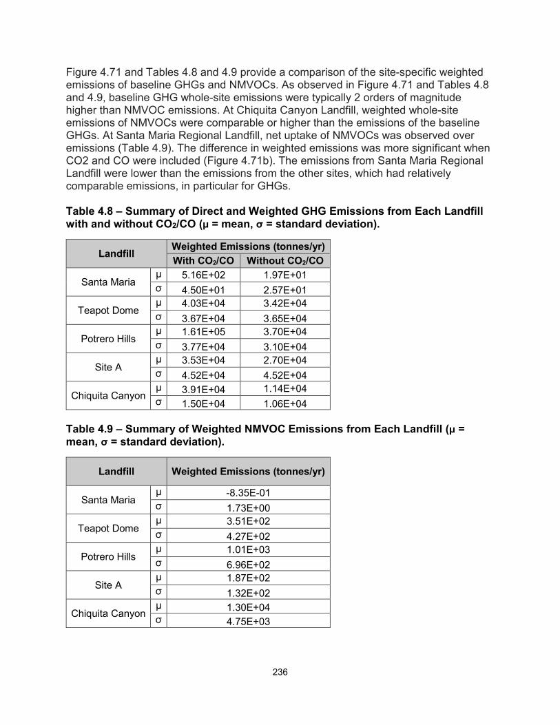
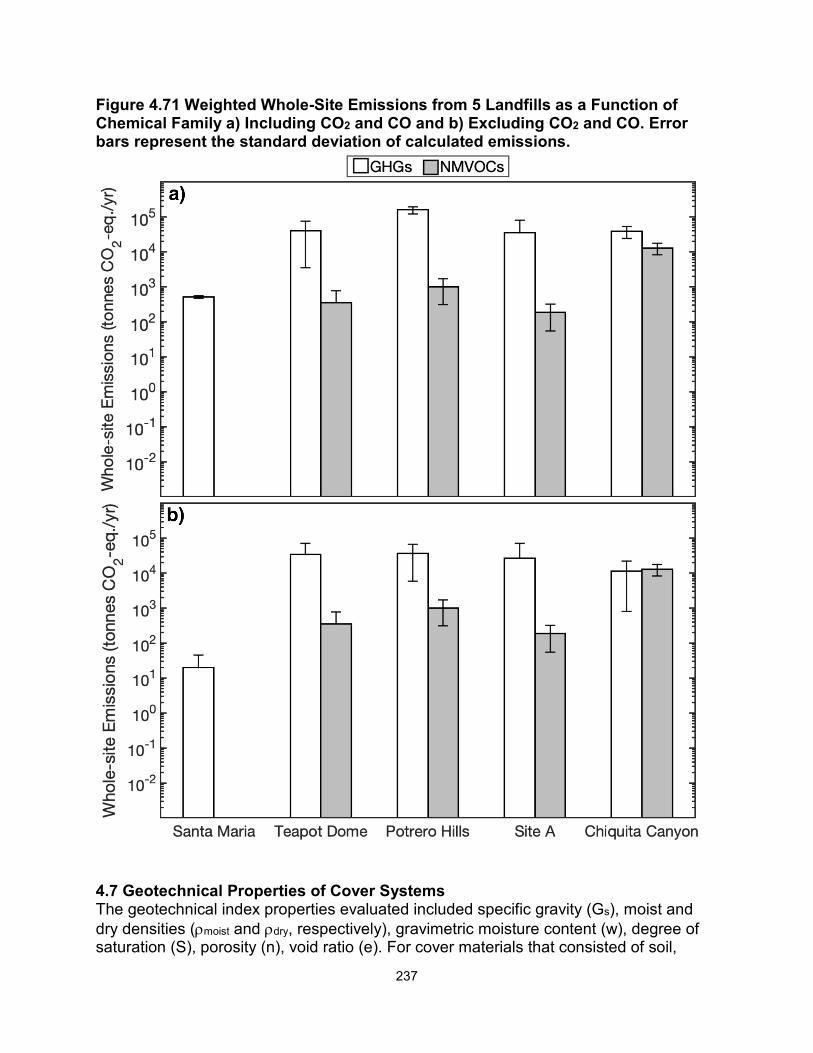
Figure 4.71 and Tables 4.8 and 4.9 provide a comparison of the site-specific weighted emissions of baseline GHGs and NMVOCs. As observed in Figure 4.71 and Tables 4.8 and 4.9, baseline GHG whole-site emissions were typically 2 orders of magnitude higher than NMVOC emissions. At Chiquita Canyon Landfill, weighted whole-site emissions of NMVOCs were comparable or higher than the emissions of the baseline GHGs. At Santa Maria Regional Landfill, net uptake of NMVOCs was observed over emissions (Table 4.9). The difference in weighted emissions was more significant when CO2 and CO were included (Figure 4.71b). The emissions from Santa Maria Regional Landfill were lower than the emissions from the other sites, which had relatively comparable emissions, in particular for GHGs. Table 4.8 – Summary of Direct and Weighted GHG Emissions from Each Landfill with and without CO2/CO (μ = mean, σ = standard deviation).

Landfill Weighted Emissions (tonnes/yr) With CO2/CO Without CO2/CO

Santa Maria μ 5.16E+02 1.97E+01 σ 4.50E+01 2.57E+01

Teapot Dome μ 4.03E+04 3.42E+04 σ 3.67E+04 3.65E+04

Potrero Hills μ 1.61E+05 3.70E+04 σ 3.77E+04 3.10E+04

Site A μ 3.53E+04 2.70E+04 σ 4.52E+04 4.52E+04

Chiquita Canyon μ 3.91E+04 1.14E+04 σ 1.50E+04 1.06E+04

Table 4.9 – Summary of Weighted NMVOC Emissions from Each Landfill (μ = mean, σ = standard deviation).

Landfill Weighted Emissions (tonnes/yr)

Santa Maria μ -8.35E-01 σ 1.73E+00

Teapot Dome μ 3.51E+02 σ 4.27E+02

Potrero Hills μ 1.01E+03 σ 6.96E+02

Site A μ 1.87E+02 σ 1.32E+02

Chiquita Canyon μ 1.30E+04 σ 4.75E+03

237

Figure 4.71 Weighted Whole-Site Emissions from 5 Landfills as a Function of Chemical Family a) Including CO2 and CO and b) Excluding CO2 and CO. Error bars represent the standard deviation of calculated emissions.

4.7 Geotechnical Properties of Cover Systems The geotechnical index properties evaluated included specific gravity (Gs), moist and dry densities (ρmoist and ρdry, respectively), gravimetric moisture content (w), degree of saturation (S), porosity (n), void ratio (e). For cover materials that consisted of soil,

238

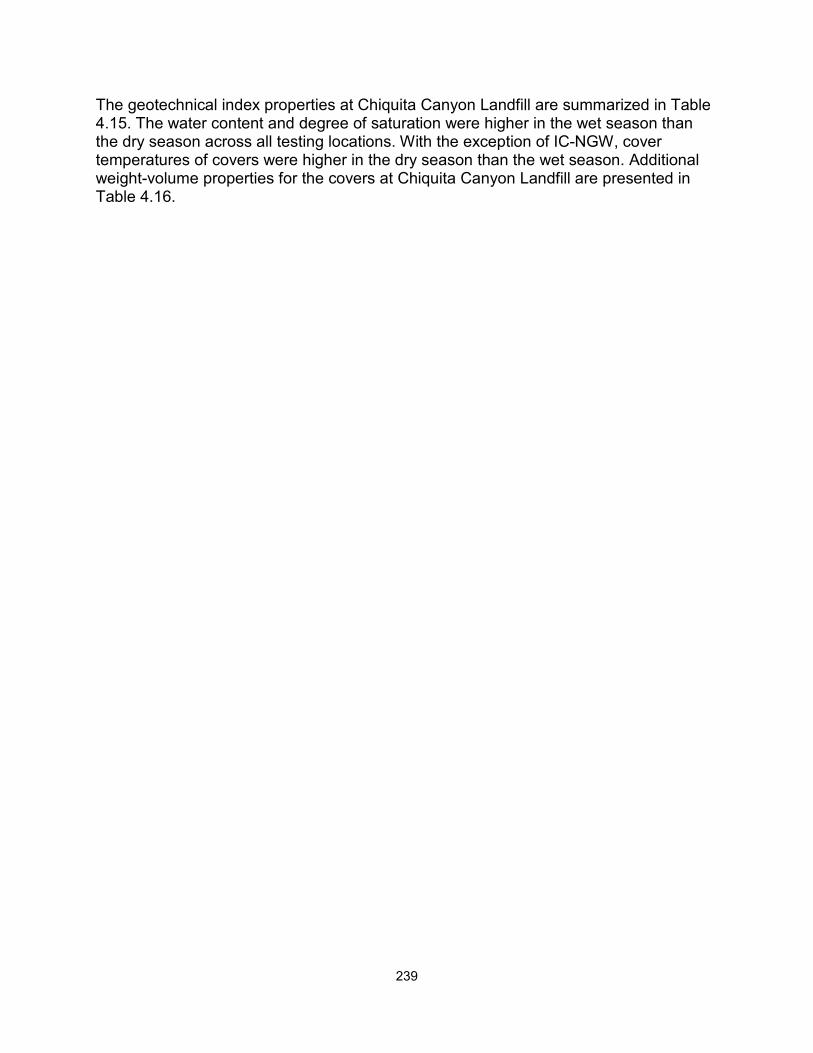
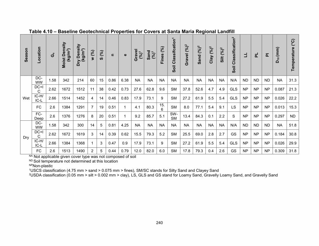
gravel content (USCS classification), sand content (USCS classification), fines content (USCS classification), silt content (USDA classification), and clay content (USDA classification) were also included, respective of season as appropriate. In addition, Atterberg limits (PL, LL, and PI) were determined as appropriate. Cover temperatures measured in-situ during field testing within the chamber footprint were evaluated. An additional set of geotechnical characteristics (10 total) were further calculated by incorporating the cover thickness, chamber area (1 m2), and weight-volume relationships of the cover materials to quantify the column of cover material present directly beneath the testing location. These weight-volume characteristics included the mass of solids (Ms), mass of water (Mw), total mass (MT), volume of solids (Vs), volume of water (Vw), volume of voids (Vv, i.e., volume of air + volume of water), volume of air (Va). In addition, volumetric solids content (θs), volumetric water content (θw), and volumetric air content (θa) were calculated by dividing the corresponding volume of solids, water or air by the total volume as applicable. Furthermore, waste ages and waste column heights directly beneath the column testing locations were determined through interpretation of historic topographic maps obtained from site records. An average waste age for the entire waste column beneath the testing location was determined. The geotechnical index properties at Santa Maria Regional Landfill are summarized in Table 4.7. The water content and degree of saturation were higher in the wet season than the dry season across all testing locations. Cover temperatures were generally warmer in the dry season than the wet season, and greater for alternative daily cover materials, such as the wood waste locations than the soil covers (Table 4.7), indicative of biological decay of the wood waste materials. Additional weight-volume properties for the covers at Santa Maria Regional Landfill are presented in Table 4.8. The geotechnical index properties at Teapot Dome Landfill are summarized in Table 4.9. The water content and degree of saturation were generally higher in the wet season than the dry season across all testing locations. Cover temperatures were generally significantly warmer in the dry season than the wet season. Additional weight-volume properties for the covers at Teapot Dome Landfill are presented in Table 4.10. The geotechnical index properties at Potrero Hills Landfill are summarized in Table 4.11. The water content and degree of saturation were higher in the wet season than the dry season across all testing locations. Cover temperatures for daily covers were generally significantly higher in the wet season than the dry season. Additional weight-volume properties for the covers at Potrero Hills Landfill are presented in Table 4.12. The geotechnical index properties at Site A Landfill are summarized in Table 4.13. The water content and degree of saturation were higher in the wet season than the dry season across all testing locations. Cover temperatures of covers were higher in the dry season than the wet season. Additional weight-volume properties for the covers at Potrero Hills Landfill are presented in Table 4.14.

239

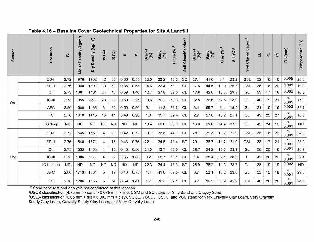
The geotechnical index properties at Chiquita Canyon Landfill are summarized in Table 4.15. The water content and degree of saturation were higher in the wet season than the dry season across all testing locations. With the exception of IC-NGW, cover temperatures of covers were higher in the dry season than the wet season. Additional weight-volume properties for the covers at Chiquita Canyon Landfill are presented in Table 4.16.

240

Table 4.10 – Baseline Geotechnical Properties for Covers at Santa Maria Regional Landfill Se

ason

Loca

tion

Gs

Moi

st D

ensi

ty

(kg/

m3 )

Dry

Den

sity

(k

g/m

3 )

w (%

)

S (%

)

n e

Gra

vel

(%)1

Sand

(%

)1

Fine

s (%

)

Soil

Cla

ssifc

atio

n1

Gra

vel (

%)2

Sand

(%)2

Cla

y (%

)2

Silt

(%)2

Soil

Cla

ssifi

catio

n2

LL

PL

PI

D10

(mm

)

Tem

pera

ture

(°C

)

Wet

DC-WW 1.58 342 214 60 15 0.86 6.38 NA NA NA NA NA NA NA NA N/A ND ND ND NA 31.3

DC+IC 2.62 1672 1512 11 38 0.42 0.73 27.6 62.8 9.6 SM 37.8 52.6 4.7 4.9 GLS NP NP NP 0.087 21.3

IC-H/ IC-L 2.66 1514 1452 4 14 0.46 0.83 17.9 73.1 9 SM 27.2 61.9 5.5 5.4 GLS NP NP NP 0.026 22.2

FC 2.6 1384 1291 7 19 0.51 1 4.1 80.3 15.6 SM 8.0 77.1 5.4 9.1 LS NP NP NP 0.013 15.3

FC-Deep 2.6 1376 1276 8 20 0.51 1 9.2 85.7 5.1 SW-

SM 13.4 84.3 0.1 2.2 S NP NP NP 0.297 ND

Dry

DC-WW 1.58 342 300 14 5 0.81 4.25 NA NA NA NA NA NA NA NA N/A ND ND ND NA 51.8

DC+IC 2.62 1672 1619 3 14 0.39 0.62 15.5 79.3 5.2 SM 25.5 69.0 2.8 2.7 GS NP NP NP 0.184 30.8

IC-H/ IC-L 2.66 1384 1368 1 3 0.47 0.9 17.9 73.1 9 SM 27.2 61.9 5.5 5.4 GLS NP NP NP 0.026 29.9

FC 2.6 1513 1490 2 5 0.44 0.79 12.0 82.0 6.0 SM 17.8 79.3 0.4 2.6 GS NP NP NP 0.309 31.8 NA Not applicable given cover type was not composed of soil ND Soil temperature not determined at this location NPNon-plastic 1USCS classification (4.75 mm > sand > 0.075 mm > fines), SM/SC stands for Silty Sand and Clayey Sand 2USDA classification (0.05 mm > silt > 0.002 mm > clay), LS, GLS and GS stand for Loamy Sand, Gravelly Loamy Sand, and Gravelly Sand

241

Table 4.11 – Composite Geotechnical Properties for Covers at Santa Maria Regional Landfill

Seas

on

Loca

tion

Ms (k

g)

Mw

(kg)

MT (k

g)

V s (m

3 )

V w (m

3 )

V v (m

3 )

V a (m

3 )

θ s

θ w

θ a

Was

te

Age

(y

ears

)

Col

umn

Hei

ght (

m)

Wet

DC-WW 59.9 36.0 95.9 0.038 0.036 0.241 0.205 0.135 0.129 0.731 16.9 16.5 DC+IC 1194.5 131.4 1325.9 0.455 0.126 0.332 0.206 0.575 0.160 0.260 15.7 17.1

IC-H/IC-L 987.4 39.5 1026.9 0.377 0.044 0.313 0.269 0.554 0.064 0.396 8.28 22.5 FC 936.4 58.8 995.2 0.353 0.057 0.324 0.267 0.519 0.084 0.393 35 15.9

Dry

DC-WW 84.0 11.8 95.8 0.053 0.011 0.227 0.215 0.191 0.041 0.770 15.0 21.6 DC+IC 1279.0 38.4 1317.4 0.497 0.043 0.308 0.265 0.629 0.055 0.335 15.7 17.1

IC-H/IC-L 930.2 9.3 939.5 0.355 0.010 0.320 0.310 0.522 0.014 0.456 8.28 22.5 FC 930.2 9.3 939.5 0.355 0.010 0.320 0.310 0.522 0.014 0.456 35 15.9

242

Table 4.12 – Baseline Cover Geotechnical Properties for Teapot Dome Landfill Se

ason

Loca

tion

Gs

Moi

st D

ensi

ty

(kg/

m3 )

Dry

Den

sity

(k

g/m

3 )

w (%

)

S (%

)

n e

Gra

vel

(%)1

Sand

(%

)1

Fine

s (%

)1

Soil

Cla

ssifi

catio

n1

Gra

vel

(%)2

Sand

(%

)2

Cla

y (%

)2

Silt

(%)2

Soil

Cla

ssifi

catio

n2

LL

PL

PI

D10

(mm

)

Tem

pera

ture

(°C

)

Wet

DC-S 2.76 1290 1175 10 19 0.57 1.35 1.9 67.5 30.

6 SC-SM 7.8 60.8 7.4 24.0 SL 22 17 5 0.005 15.8

IC-S+GW 2.72 1230 1065 15 30 0.6

1 1.57 2.4 37.2 60.4 CL 4.1 51.8 12.

3 31.7 SL 28 20 8 0.001 13.2

IC-N 2.74 1270 1105 15 27 0.6 1.48 0.3 72.0 28.7 SM 2.4 72.3 8.3 17.0 SL NP NP NP 0.004 13.7

IC-O 2.7 1250 1085 11 27 0.59 1.5 3.7 72.8 23.

5 SM 18.2 58.1 8.4 15.3 GSL 25 17 18 0.003 13.7

IC-W 2.77 1346 1166 15 31 0.58 1.38 0.4 58.8 40.

8 SM 2.1 60.5 11.4 26.3 SL 27 22 5 0.002 14.5

Dry

DC-GW 1.8 315 271 16 5 0.8

5 5.67 NA NA NA NA NA NA NA NA NA NA NA NA NA 29.3

IC-S+GW 2.72 1440 1339 7 20 0.5

1 1.05 1.7 58.9 39.4 SC 7.9 67.3 5.1 19.7 SL 23 15 8 0.019 30.9

IC-N 2.74 1517 1495 2 5 0.45 0.83 16.9 55.1 28 SM 24.1 58.2 6.6 11.1 GSL NP NP NP 0.007 37.2

IC-O 2.7 1214 1191 2 4 0.56 1.27 2.8 44.6 52.

6 CL 12.3 54.1 5.4 28.2 SL 30 15 15 0.011 32.5

IC-W 2.77 1266 1236 3 5 0.56 1.25 0.1 41.2 58.

7 ML 0.7 61.1 6.7 31.5 SL 23 22 1 0.008 34.9 NA Not applicable given cover type was not composed of soil NPNon-plastic 1USCS classification (4.75 mm > sand > 0.075 mm > fines), SM or SC stand for Silty Sand and Clayey Sand 2USDA classification (0.05 mm > silt > 0.002 mm > clay), GSL stands for Gravelly Sandy Loam

243

Table 4.13 – Composite Geotechnical Properties for Covers at Teapot Dome Landfill Se

ason

Loca

tion

Ms (k

g)

Mw

(kg)

MT

(kg)

V s (m

3 )

V w (m

3 )

V v (m

3 )

V a (m

3 )

θ s

θ w

θ a

Was

te A

ge

(yea

rs)

Colu

mn

Heig

ht (m

)

Wet

DC-S 223.3 22.3 245.6 0.080 0.021 0.108 0.088 0.422 0.108 0.462 21.4 26.2 IC-S+GW 447.3 67.1 514.4 0.163 0.077 0.256 0.179 0.389 0.183 0.427 27.1 24.1

IC-N 386.8 58.0 444.8 0.142 0.057 0.210 0.153 0.405 0.162 0.438 21.7 21 IC-O 846.3 93.1 939.4 0.307 0.124 0.460 0.336 0.393 0.159 0.431 30.9 4.1 IC-W 396.4 59.5 455.9 0.143 0.061 0.197 0.136 0.420 0.180 0.400 27.2 27.2

Dry

DC-GW 73.2 11.7 84.9 0.040 0.011 0.230 0.218 0.150 0.043 0.808 26.6 24.4 IC-S+GW 562.4 39.4 601.7 0.204 0.043 0.214 0.171 0.486 0.102 0.408 27.1 24.1

IC-N 523.3 10.5 533.7 0.190 0.008 0.158 0.150 0.542 0.023 0.428 21.7 21 IC-O 929.0 18.6 947.6 0.344 0.017 0.437 0.419 0.441 0.022 0.538 30.9 4.1 IC-W 420.2 12.6 432.8 0.152 0.010 0.190 0.181 0.448 0.028 0.532 27.2 27.2

244

Table 4.14 – Baseline Cover Geotechnical Properties for Potrero Hills Landfill

Seas

on

Loca

tion

Gs

Moi

st D

ensi

ty (k

g/m

3 )

Dry

Den

sity

(kg/

m3 )

w (%

)

S (%

)

n e

Gra

vel

(%)1

Sand

(%

)1

Fine

s (%

)1

Soil

Cla

ssifi

catio

n1

Gra

vel

(%)2

Sand

(%

)2

Cla

y (%

)2

Silt

(%)2

Soil

Cla

ssifi

catio

n2

LL

PL

PI

D10

(mm

)

Tem

pera

ture

(°C

)

Wet

DC-AF 1.73 430 337 25 11 0.8 4.14 NA NA NA NA NA NA NA NA NA NA NA NA NA 43.6

DC-GW 1.35 200 148 37 5 0.89 7.96 NA NA NA NA NA NA NA NA NA NA NA NA NA 55.9

DC-C+D 1.2 200 146 30 6 0.88 7.25 NA NA NA NA NA NA NA NA NA NA NA NA NA 48.2

IC-BM 2.75 1735 1525 13 46 0.45 0.8 24.0 31.1 45.0 SC 28.5 42.0 8.6 20.9 GSL 30 18 12 0.005 19.8

IC-C1 2.65 1341 1074 24 44 0.61 1.53 3.2 29.1 67.7 CH 5.2 49.1 10.1 35.6 L 51 22 29 0.002 16.7 IC-C1 deep 2.65 1075 840 28 34 0.68 2.16 0.5 15.0 84.5 CH 2.5 27.9 26.1 43.4 CL 51 23 28 <0.001 ND

FC 2.72 1711 1451 17 55 0.47 0.88 1.1 18.3 80.6 CH 2.0 27.6 36.4 34.0 CL 56 27 29 <0.001 16.4

Dry

DC-AF 1.73 168 161 0.7 0.41 0.75 3.05 NA NA NA NA NA NA NA NA NA NA NA NA NA 38.2

DC-GW 1.35 170 164 4 0.86 0.86 6.01 NA NA NA NA NA NA NA NA NA NA NA NA NA 31.7

IC-S 2.73 1711 1602 6 26 0.42 0.71 24.0 31.1 45.0 SC 28.5 33.5 18.9 19.1 GSCL 54 21 33 <0.001 24.9

IC-BM 2.75 1546 1463 6 17 0.47 0.89 7.1 60.7 32.2 SC 11.9 58.3 12.3 17.5 SL 25 13 12 <0.001 30.6

IC-C1 2.65 1050 967 8 13 0.64 1.76 3.0 27.2 69.9 CH 5.7 49.6 9.4 35.3 SL 54 21 33 <0.001 26.0

FC 2.72 1141 1072 7 11 0.61 1.54 2.5 10.9 86.6 CH 3.1 19.7 36.3 41.0 CL 56 27 29 <0.001 24.5 NA Not applicable given cover type was not composed of soil ND Sand cone test and analysis not conducted at this location 1USCS classification (4.75 mm > sand > 0.075 mm > fines), SM, SC, GM, and GC stand for Silty Sand, Clayey Sand, Silty Gravel, and Clayey Gravel 2USDA classification (0.05 mm > silt > 0.002 mm > clay), SL, GC, VGC stand for Silty Loam, Gravelly Clay and Very Gravelly Clay

245

Table 4.15 – Composite Geotechnical Properties for Covers at Potrero Hills Landfill Se

ason

Loca

tion

Ms (k

g)

Mw

(kg)

MT

(kg)

V s (m

3 )

V w (m

3 )

V v (m

3 )

V a (m

3 )

θ s

θ w

θ a

Was

te A

ge

(yea

rs)

Colu

mn

Heig

ht (m

)

Wet

DC-AF 148.3 37.1 185.4 0.085 0.039 0.352 0.313 0.193 0.088 0.712 15.1 49.2 DC-GW 77.0 28.5 105.4 0.058 0.023 0.463 0.440 0.112 0.045 0.846 12.7 50.2 DC-C+D 30.7 9.2 39.9 0.025 0.011 0.185 0.174 0.121 0.053 0.827 13.3 43.9 IC-BM 1982.5 257.7 2240.2 0.731 0.269 0.585 0.316 0.563 0.207 0.243 12.7 45.1 IC-C1 902.2 216.5 1118.7 0.335 0.225 0.512 0.287 0.399 0.268 0.342 19.7 19.4

FC 1741.2 296.0 2037.2 0.641 0.310 0.564 0.254 0.534 0.259 0.212 18.0 13.7

Dry

DC-AF 122.4 0.9 123.2 0.187 0.002 0.570 0.568 0.246 0.003 0.747 13.5 42.5 DC-GW 50.8 2.0 52.9 0.044 0.002 0.267 0.264 0.143 0.007 0.853 13.2 41.4

IC-S 4645.8 278.7 4924.5 1.715 0.317 1.218 0.901 0.592 0.109 0.311 15.1 50.1 IC-BM 1901.9 114.1 2016.0 0.687 0.104 0.611 0.507 0.528 0.080 0.390 12.7 45.1 IC-C1 812.3 65.0 877.3 0.305 0.070 0.538 0.468 0.364 0.083 0.557 19.7 19.4

FC 1286.4 90.0 1376.4 0.475 0.081 0.732 0.651 0.396 0.067 0.543 18.0 13.7

246

Table 4.16 – Baseline Cover Geotechnical Properties for Site A Landfill

Seas

on

Loca

tion

Gs

Moi

st D

ensi

ty (k

g/m

3 )

Dry

Den

sity

(kg/

m3 )

w (%

)

S (%

)

n e

Gra

vel

(%)1

Sand

(%

)1

Fine

s (%

)1

Soil

Cla

ssifi

catio

n1

Gra

vel

(%)2

Sand

(%

)2

Cla

y (%

)2

Silt

(%)2

Soil

Cla

ssifi

catio

n2

LL

PL

PI

D10

(mm

)

Tem

pera

ture

(°C

)

Wet

ED-II 2.72 1976 1762 12 60 0.36 0.55 20.5 33.2 46.3 SC 27.1 41.6 8.1 23.2 GSL 32 16 16 0.005 20.8 ED-III 2.76 1980 1801 10 51 0.35 0.53 14.6 32.4 53.1 CL 17.8 44.5 11.9 25.7 GSL 36 16 20 0.001 19.9 IC-II 2.73 1381 1101 24 45 0.59 1.46 12.7 27.8 59.5 CL 17.8 42.0 10.3 29.8 GL 33 17 16 0.002 10.3 IC-III 2.73 1055 853 23 29 0.69 2.25 10.6 30.2 59.3 CL 12.8 36.6 32.5 18.0 CL 40 19 21 <

0.001 15.1

AFC 2.86 1600 1438 8 32 0.50 0.96 5.1 11.3 83.6 CL 3.4 69.7 8.4 18.5 SL 31 15 16 0.003 23.7 FC 2.78 1618 1415 15 41 0.49 0.98 1.8 15.7 82.4 CL 2.7 27.0 45.2 25.1 CL 49 22 27 <

0.001 16.8

FC deep ND ND ND ND ND ND ND 10.4 20.6 69.0 CL 16.0 21.8 24.4 37.9 CL 42 24 18 < 0.001 ND

Dry

ED-II 2.72 1645 1581 4 21 0.42 0.72 19.1 36.8 44.1 CL 28.1 39.3 10.7 21.9 GSL 38 16 22 < 0.001 24.0

ED-III 2.76 1640 1571 4 16 0.43 0.76 22.1 34.5 43.4 SC 29.1 38.7 11.2 21.0 GSL 38 17 21 < 0.001 23.9

IC-II 2.73 1535 1468 4 15 0.46 0.86 24.3 13.7 62.0 CL 29.7 24.2 16.3 29.9 GL 36 20 16 0.001 28.9 IC-III 2.73 1006 963 4 6 0.65 1.85 0.2 28.7 71.1 CL 1.4 38.4 22.1 38.0 L 42 20 22 <

0.001 27.4

IC-III deep ND ND ND ND ND ND ND 22.3 34.4 43.3 SC 28.9 36.2 11.3 23.7 GL 38 19 19 0.002 ND AFC 2.86 1713 1631 5 19 0.43 0.75 1.4 41.0 57.5 CL 3.7 53.1 15.2 29.6 SL 33 15 18 <

0.001 29.5

FC 2.78 1206 1155 5 9 0.59 1.41 1.7 9.2 89.1 CL 3.7 19.5 30.9 45.9 GSL 46 26 20 < 0.001 24.8

ND Sand cone test and analysis not conducted at this location 1USCS classification (4.75 mm > sand > 0.075 mm > fines), SM and SC stand for Silty Sand and Clayey Sand 2USDA classification (0.05 mm > silt > 0.002 mm > clay), VGCL, VGSCL, GSCL, and VGL stand for Very Gravelly Clay Loam, Very Gravelly Sandy Clay Loam, Gravelly Sandy Clay Loam, and Very Gravelly Loam

247

Table 4.17 – Composite Geotechnical Properties for Covers at Site A Landfill Se

ason

Loca

tion

Ms (k

g)

Mw

(kg)

MT

(kg)

V s (m

3 )

V w (m

3 )

V v (m

3 )

V a (m

3 )

θ s

θ w

θ a

Was

te A

ge

(yea

rs)

Colu

mn

Heig

ht (m

)

Wet

ED-II 4052.6 486.3 4538.9 1.505 0.497 0.828 0.331 0.655 0.216 0.144 28.1 109 ED-III 2503.4 250.3 2753.7 0.918 0.248 0.487 0.238 0.660 0.179 0.172 27.8 113 IC-II 429.4 103.1 532.4 0.158 0.104 0.230 0.127 0.404 0.266 0.325 27.3 117 IC-III 1288.0 296.2 1584.3 0.463 0.302 1.042 0.740 0.307 0.200 0.490 29.0 66.5 AFC 1725.6 138.0 1863.6 0.625 0.192 0.600 0.408 0.521 0.160 0.340 29.0 108 FC 2971.5 445.7 3417.2 1.050 0.422 1.029 0.607 0.500 0.201 0.289 29.0 47.6

Dry

ED-II 1581.0 63.2 1644.2 0.806 0.101 0.584 0.482 0.580 0.073 0.347 24.2 110 ED-III 502.7 20.1 522.8 0.182 0.022 0.138 0.116 0.569 0.069 0.362 29.0 112 IC-II 572.5 22.9 595.4 0.209 0.027 0.179 0.152 0.535 0.069 0.391 27.3 117 IC-III 1454.1 58.2 1512.3 0.531 0.059 0.982 0.923 0.351 0.039 0.611 29.0 66.5 AFC 1988.2 99.4 2087.6 0.695 0.099 0.523 0.425 0.573 0.082 0.348 29.0 108.0 FC 2425.5 121.3 2546.8 0.879 0.112 1.239 1.127 0.418 0.053 0.537 29.0 47.6

248

Table 4.18 – Baseline Cover Geotechnical Properties for Chiquita Canyon Landfill Se

ason

Loca

tion

Gs

Moi

st D

ensi

ty (k

g/m

3 )

Dry

Den

sity

(kg/

m3 )

w (%

)

S (%

)

n e

Gra

vel

(%)1

Sand

(%

)1

Fine

s (%

)1

Soil

Cla

ssifi

catio

n1

Gra

vel

(%)2

Sand

(%

)2

Cla

y (%

)2

Silt

(%)2

Soil

Cla

ssifi

catio

n2

LL

PL

PI

D10

(mm

)

Tem

pera

ture

(°C

)

Wet

DC-Cl 2.44 1116 1069 7 14 0.57 1.3 24.9 50.0 39.8 SC 29.2 54.4 3.6 12.8 GSL 36 21 15 0.047 22.9

DC-Co 2.69 1671 1515 10 35 0.43 0.78 8.4 57.1 34.5 SC- SM 12.4 65.7 5.1 16.8 LS 25 19 6 0.028 22.8

IC-S 2.76 1427 1369 4 11 0.51 1 4.0 51.8 44.2 SC 7.6 66.1 6.1 20.2 SL 29 19 10 0.011 18.4

IC-W 2.72 1500 1415 6 17 0.47 0.93 2.6 44.9 52.5 CL 6.1 58.2 8.6 27.1 SL 31 18 13 0.004 20.4

IC-OGW 2.12 334 267 27 9 0.87 7 NA NA NA NA NA NA NA NA NA NA NA NA NA 41.6

IC-NGW 1.65 153 106 62 6 0.95 16 NA NA NA NA NA NA NA NA NA NA NA NA NA 39.6

FC 2.73 1172 1143 3 5 0.58 1.4 4.2 55.8 40.0 SC 8.6 66.0 5.1 20.4 SL 32 21 11 0.018 23.4

Dry

DC-Cl 2.44 1481 1428 3 13 0.42 0.71 18.3 48.8 32.9 SC 16.2 66.4 1.4 15.9 GLS 27 20 7 0.003 32.5

DC-Co 2.69 1414 1378 3 7 0.49 0.96 5.1 84.6 10.3 SP-SM 28.0 48.3 9.5 14.2 GSL NP NP NP 0.074 36.4

IC-S 2.76 1581 1551 3 7 0.46 0.8 10.3 50.3 39.4 SC 13.3 60.5 5.4 20.8 SL 29 18 11 0.011 33.4

IC-W 2.72 1276 1238 3 7 0.55 1.21 14.0 46.7 39.3 SC 17.4 56.5 5.4 20.7 GSL 28 18 10 0.011 33.0

IC-OGW 2.12 400 383 4 2 0.82 4.52 NA NA NA NA NA NA NA NA NA NA NA NA NA 45.7

IC-NGW 1.65 317 307 5 2 0.81 4.47 NA NA NA NA NA NA NA NA NA NA NA NA NA 37.3

FC 2.73 1432 1414 1 4 0.48 0.93 3.8 57.3 38.9 SC 8.5 66.8 4.9 19.8 SL 27 19 8 0.018 41.1 NA Not applicable given cover type was not composed of soil 1USCS classification (4.75 mm > sand > 0.075 mm > fines), SM and SC stand for Silty Sand and Clayey Sand 2USDA classification (0.05 mm > silt > 0.002 mm > clay), GSL and VGSL stand for Gravelly Sandy Loam and Very Gravelly Sandy Loam

249

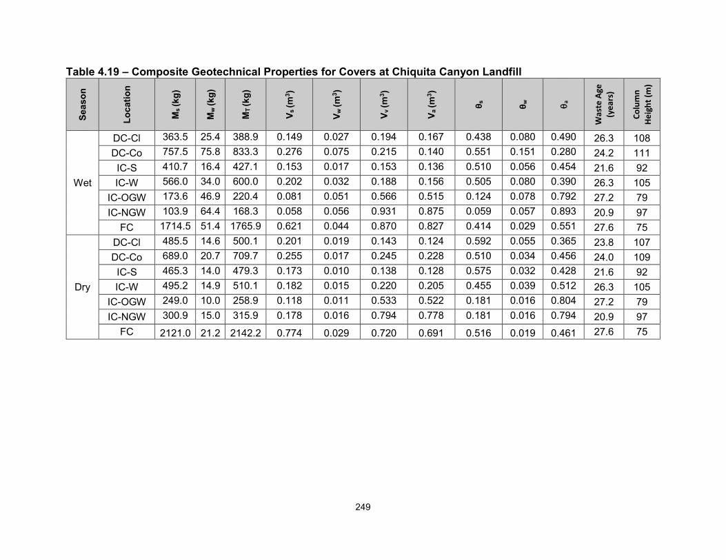
Table 4.19 – Composite Geotechnical Properties for Covers at Chiquita Canyon Landfill Se

ason

Loca

tion

Ms (k

g)

Mw

(kg)

MT

(kg)

V s (m

3 )

V w (m

3 )

V v (m

3 )

V a (m

3 )

θ s

θ w

θ a

Was

te A

ge

(yea

rs)

Colu

mn

Heig

ht (m

)

Wet

DC-Cl 363.5 25.4 388.9 0.149 0.027 0.194 0.167 0.438 0.080 0.490 26.3 108 DC-Co 757.5 75.8 833.3 0.276 0.075 0.215 0.140 0.551 0.151 0.280 24.2 111 IC-S 410.7 16.4 427.1 0.153 0.017 0.153 0.136 0.510 0.056 0.454 21.6 92 IC-W 566.0 34.0 600.0 0.202 0.032 0.188 0.156 0.505 0.080 0.390 26.3 105

IC-OGW 173.6 46.9 220.4 0.081 0.051 0.566 0.515 0.124 0.078 0.792 27.2 79 IC-NGW 103.9 64.4 168.3 0.058 0.056 0.931 0.875 0.059 0.057 0.893 20.9 97

FC 1714.5 51.4 1765.9 0.621 0.044 0.870 0.827 0.414 0.029 0.551 27.6 75

Dry

DC-Cl 485.5 14.6 500.1 0.201 0.019 0.143 0.124 0.592 0.055 0.365 23.8 107 DC-Co 689.0 20.7 709.7 0.255 0.017 0.245 0.228 0.510 0.034 0.456 24.0 109 IC-S 465.3 14.0 479.3 0.173 0.010 0.138 0.128 0.575 0.032 0.428 21.6 92 IC-W 495.2 14.9 510.1 0.182 0.015 0.220 0.205 0.455 0.039 0.512 26.3 105

IC-OGW 249.0 10.0 258.9 0.118 0.011 0.533 0.522 0.181 0.016 0.804 27.2 79 IC-NGW 300.9 15.0 315.9 0.178 0.016 0.794 0.778 0.181 0.016 0.794 20.9 97

FC 2121.0 21.2 2142.2 0.774 0.029 0.720 0.691 0.516 0.019 0.461 27.6 75

250

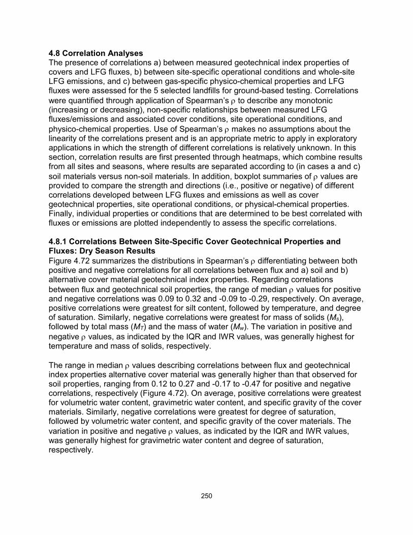
4.8 Correlation Analyses The presence of correlations a) between measured geotechnical index properties of covers and LFG fluxes, b) between site-specific operational conditions and whole-site LFG emissions, and c) between gas-specific physico-chemical properties and LFG fluxes were assessed for the 5 selected landfills for ground-based testing. Correlations were quantified through application of Spearman’s ρ to describe any monotonic (increasing or decreasing), non-specific relationships between measured LFG fluxes/emissions and associated cover conditions, site operational conditions, and physico-chemical properties. Use of Spearman’s ρ makes no assumptions about the linearity of the correlations present and is an appropriate metric to apply in exploratory applications in which the strength of different correlations is relatively unknown. In this section, correlation results are first presented through heatmaps, which combine results from all sites and seasons, where results are separated according to (in cases a and c) soil materials versus non-soil materials. In addition, boxplot summaries of ρ values are provided to compare the strength and directions (i.e., positive or negative) of different correlations developed between LFG fluxes and emissions as well as cover geotechnical properties, site operational conditions, or physical-chemical properties. Finally, individual properties or conditions that are determined to be best correlated with fluxes or emissions are plotted independently to assess the specific correlations. 4.8.1 Correlations Between Site-Specific Cover Geotechnical Properties and Fluxes: Dry Season Results Figure 4.72 summarizes the distributions in Spearman’s ρ differentiating between both positive and negative correlations for all correlations between flux and a) soil and b) alternative cover material geotechnical index properties. Regarding correlations between flux and geotechnical soil properties, the range of median ρ values for positive and negative correlations was 0.09 to 0.32 and -0.09 to -0.29, respectively. On average, positive correlations were greatest for silt content, followed by temperature, and degree of saturation. Similarly, negative correlations were greatest for mass of solids (Ms), followed by total mass (MT) and the mass of water (Mw). The variation in positive and negative ρ values, as indicated by the IQR and IWR values, was generally highest for temperature and mass of solids, respectively. The range in median ρ values describing correlations between flux and geotechnical index properties alternative cover material was generally higher than that observed for soil properties, ranging from 0.12 to 0.27 and -0.17 to -0.47 for positive and negative correlations, respectively (Figure 4.72). On average, positive correlations were greatest for volumetric water content, gravimetric water content, and specific gravity of the cover materials. Similarly, negative correlations were greatest for degree of saturation, followed by volumetric water content, and specific gravity of the cover materials. The variation in positive and negative ρ values, as indicated by the IQR and IWR values, was generally highest for gravimetric water content and degree of saturation, respectively.

251

Figure 4.72 Distributions of Spearman’s ρ (both positive and negative correlations) Describing Correlations between Geotechnical a) Soil and b) Alternative Cover Material Properties and Measured Fluxes for the Dry Season across all Landfill Sites and Cover Categories.

The strength and direction of non-linear correlations evaluated between cover geotechnical index properties and measured fluxes was presented as a function of chemical family in heatmap format (Figures 4.73 and 4.74). Results presented in both figures depict stronger and weaker correlations as darker red/purple and lighter blue shading. The direction of correlations (positive or negative) are indicated by the presence or absence of a down arrow to indicate negative. Correlations between flux and soil or alternative cover materials are presented in Figures 4.73 and 4.74, respectively, where the median of the Spearman’s correlation coefficients of all chemicals within a given family is presented. Regarding correlations between flux and

252

cover geotechnical soil properties, there was a general dearth of strong correlations (ρ > 0.5) observed, as indicated by the lack of yellow to red coloring on the heatmap. The majority of the coloring on the heatmap ranges from light blue to dark blue, indicating moderate, non-linear correlations (0.3 <ρ < 0.5) were observed between select geotechnical properties and several chemical families. In general, the monoterpenes, ketones, GHGs and organic alkyl nitrates demonstrated the greatest number and magnitude of moderate to strong non-linear correlations out of the chemical families reviewed (Figure 4.73). Based on results presented in the heatmap, correlations were generally strongest for Ms, MT, Vs, Vv, Va, silt content, and temperature. In addition, the direction of the correlation for these moderate to strong correlations was mostly negative, with the exception of silt content and temperature of the tested materials. Results presented in Figure 4.74 indicated that there were more moderate to strong correlations observed between flux and alternative cover material geotechnical index properties as compared to soil geotechnical index properties. In select cases, strong correlations were observed, with median values for certain chemical families on the order of 0.80 (negative direction). The alcohols, monoterpenes, and aromatics were generally associated with the greatest number and magnitude of moderate to strong correlations (Figure 4.74). Specific gravity, dry and wet densities, porosity, void ration, mass of solids, volume of solids, volume of voids, volume of air, and temperature were the geotechnical properties demonstrating the strongest degree of correlation across all chemical families. Similar to results obtained for the soil properties, the majority of these moderate to strong correlations were negative, aside from temperature, porosity, void ratio, and specific gravity (Figure 4.74). The relative shape and statistical dependency of the strongest non-linear correlations observed between flux and soil/alternative cover geotechnical index properties is examined in further detail in Figures 4.75 and 4.76. In both Figures, the flux is plotted as a function of the cover properties showing the highest a) positive and b) negative strength of correlation. When all of the chemical species within the chemical family associated with the highest mean ρ values are plotted together, a fair amount of scatter was observed (Figures 4.75 and 4.76). However, when flux is plotted on a logarithmic scale, the trends are readily apparent. In general, the negative correlations observed in Figure 4.75b are more discernible than the positive correlations presented in Figure 4.75a.

253

Figure 4.73 Strength and Direction of Non-linear Correlations between Cover Soil Geotechnical Properties and Measured Fluxes for the Dry Season across all Landfills, Cover Categories, and Cover Soil Types. Median Values of Spearman’s Correlation Coefficient are Presented by Chemical Family (black triangle indicates negative correlations and color bar represents the magnitude of Spearman’s correlation coefficient).

254

Figure 4.74 Strength and Direction of Non-linear Correlations between Alternative Cover Material Geotechnical Properties and Measured Fluxes for the Dry Season across all Landfills, Cover Categories, and Alternative Cover Types. Median Values of Spearman’s Correlation Coefficient are Presented by Chemical Family (black triangle indicates negative correlations and color bar represents the magnitude of Spearman’s correlation coefficient).

255

Figure 4.75 Summary of the Strongest Three (from left to right) a) Positive and b) Negative Correlations Observed Between Flux and Cover Soil Geotechnical Properties in the Dry Season. Results are Plotted for all Chemical Species within a Given Family, Differentiated by Color (negative fluxes are omitted since the y-axis is logarithmic scaling).

256

Figure 4.76 Summary of the Strongest Three (from left to right) a) Positive and b) Negative Correlations Observed between Flux and Alternative Cover Material Geotechnical Properties in the Dry Season. Results are Plotted for all Chemical Species within a Given Family, Differentiated by Color (negative fluxes are omitted since the y-axis is logarithmic scaling).

257

4.8.2 Summary of Correlations Between Site-Specific Cover Geotechnical Properties and Fluxes: Wet Season Results The distributions in Spearman’s ρ for both positive and negative correlations between flux and a) soil and b) alternative cover material geotechnical properties are presented in Figure 4.77. Regarding correlations between flux and soil geotechnical properties, the range in median ρ values for positive and negative correlations was 0.04 to 0.24 and -0.11 to -0.37, respectively. Positive correlations were greatest for silt content, followed by temperature, and dry density (ρd). Negative correlations were greatest for mass of solids (Ms), followed by volume of air (Va) and total mass of solids and water (MT). The variation in positive and negative ρ values, as indicated by the IQR and IWR values, was generally highest for temperature and water content, respectively. The range in median ρ values describing correlations between flux and alternative cover geotechnical index properties was generally higher than that observed for soil properties, ranging from 0.15 to 0.60 and -0.20 to -0.55 for positive and negative correlations, respectively (Figure 4.77b). On average, positive correlations were greatest for temperature, specific gravity (Gs), and volumetric air content (θa) of the cover materials. In contrast, negative correlations were greatest for mass of solids (Ms), followed by total mass (MT), and specific gravity (Gs). The variation in positive and negative ρ values, as indicated by the IQR and IWR values, was generally highest for porosity/void ratio and specific gravity, respectively. For the wet season, the strength and direction of non-linear correlations evaluated between cover geotechnical index properties and measured fluxes was presented as a function of chemical family in heatmap format (Figures 4.78 and 4.79). Similar to dry season, moderate, non-linear correlations (0.3 <ρ < 0.5) were observed between select geotechnical index properties and flux for several chemical families, as indicated by the light green to dark green coloring. In general, the F-gases, halogenated hydrocarbons, alkanes, and alkenes demonstrated the greatest number and magnitude of moderate to strong non-linear correlations (Figure 4.78). This result is distinctly different than the dry season, where the alcohols, ketones, and monoterpenes were associated with the highest number and magnitude of correlations. Based on results presented in the heatmap, correlations were generally strongest for the composite properties including Ms, MT, Vs, Vv, Va and, in some cases, silt content, and temperature. In addition, the direction of the correlation for these moderate to strong correlations was mostly negative, with the exceptions of silt content and temperature (Figure 4.78).

258

Figure 4.77 Distributions of Spearman’s ρ (both positive and negative correlations) Describing Correlations between Geotechnical a) Soil and b) Alternative Cover Material Properties and Measured Fluxes for the Wet Season across all Landfill Sites and Cover Categories.

Results presented in Figure 4.79 indicated that there were more moderate to strong correlations observed between flux and alternative cover material geotechnical index properties than for soils , in line with results obtained from the dry season. In select cases, there were very strong correlations observed, with median values for certain chemical families on the order of 0.80-0.90 (Gs and temperature for the monoterpenes). Unlike the soil cover results, the monoterpenes, greenhouse gases, and organic alkyl nitrates were generally associated with the greatest number and magnitude of moderate to strong correlations (Figure 4.79). Specific gravity, dry and moist densities, mass of solids, water-filled porosity, and temperature were the geotechnical properties

259

demonstrating the strongest degree of correlation across the chemical families reviewed. Similar to results obtained for the soil properties, the majority of these moderate to strong correlations were negative, aside from temperature (Figure 4.79). Compared to the soil properties in Figure 4.78, there were more positive, moderate strength correlations observed across chemical families, particularly for porosity, void ratio, water content, and volumetric air content. The relative shape and statistical dependency of the strongest non-linear correlations observed between flux and soil/alternative cover geotechnical index properties is examined in further detail in Figures 4.80 and 4.81. In both Figures, the flux is plotted as a function of the cover properties showing the highest a) positive and b) negative strength of correlation. A fair amount of scatter was observed when all of the chemical species within the chemical family associated with the highest mean ρ values are plotted together (Figures 4.80 and 4.81). The alcohol and organic alkyl nitrates were generally associated with the strongest positive median correlation values.

260

Figure 4.78 Strength and Direction of Non-linear Correlations between Cover Soil Geotechnical Properties and Measured Fluxes for the Wet Season across all Landfills, Cover Categories, and Cover Soil Types. Median values of Spearman’s Correlation Coefficient are Presented by Chemical Family (black triangle indicates negative correlations and color bar represents the magnitude of Spearman’s correlation coefficient).

261

Figure 4.79 Strength and Direction of Non-linear Correlations between Alternative Cover Material Geotechnical Properties and Measured Fluxes for the Wet Season across all Landfills, Cover Categories, and Alternative Cover Types. Median values of Spearman’s Correlation Coefficient are Presented by Chemical Family (black triangle indicates negative correlations and color bar represents the magnitude of Spearman’s correlation coefficient.

262

Figure 4.80 Summary of the Three Strongest (from left to right) a) Positive and b) Negative Correlations Observed between Flux and Cover Soil Geotechnical Properties in the Wet Season. Results are Plotted for all Chemical Species within a Given Family, Differentiated by Color (negative fluxes are omitted since the y-axis is logarithmic scaling).

263

Figure 4.81 Summary of the Three Strongest (from left to right) a) Positive and b) Negative Correlations Observed between Flux and Alternative Cover Material Geotechnical Properties in the Wet Season. Results are Plotted for all Chemical Species within a Given Family, Differentiated by Color (negative fluxes are omitted since the y-axis is logarithmic scaling).

264

4.8.3 Summary of Correlations Between Site-Specific Operational Conditions and Whole-Site Emissions Calculated annual whole-site emissions of methane and total LFG (combining all 82 chemicals) were correlated with fourteen different site-specific operational conditions. For sites in which aerial testing was conducted, the most recent average volumetric methane concentration reported in the recent CARB inventory of LFG extraction systems was used to convert methane to LFG. Correlations were conducted using direct whole-site emissions only. The site-specific operational conditions evaluated included total WIP (tonnes), average waste depth for the site (m), waste throughput (tonnes/day), areal coverage (m2), fractions of daily, intermediate and final cover (%), area of the active face (m2), annual LFG collected (m3), average LFG flow rate (m3/min), measured and modeled collection efficiencies (%), fraction of biodegradable waste materials (%, B0), and the age of the landfill (years). In addition, site specific climatic conditions including annual precipitation (mm) and daily average temperature (°C) were analyzed. Waste depth, waste throughput, areal coverage, fractions of daily, intermediate, and final cover, active face area, average LFG flow rate, and site age were reported by landfill operational staff from an initial survey of landfill characteristics, summarized in Section 2, and represent recent site conditions (2017-2019). WIP was determined from site records. The LFG collected (year 2018) was obtained from the latest CARB statewide inventory conducted on LFG collection systems. Modeled LFG collection efficiencies were obtained based on methodology described in Section 3.8, using default and refined estimates of LandGEM parameter values. Climatic data was summarized from 30-year averages (Andersland and Ladanyi 1994) collected from the nearest monitoring station and downloaded from the NOAA online database. Lastly, B0 values were predicted for each landfill jurisdiction using CalRecycle’s online web application, as reviewed in Section 4.8. Non-linear correlation coefficients determined between landfill characteristics and direct emissions of methane or total LFG are summarized in Table 4.18. In aerial measurements, strong correlations (0.73 to 0.84) were observed between emissions and WIP, waste throughput, areal coverage, and waste depth for methane. The strong correlations were all positive, indicating that emissions are expected to increase with the scale of landfill operations. In ground measurements, strong correlations were observed between emissions and the individual cover areas for methane. The correlations were positive or daily and intermediate covers, indicating increases in methane emissions with increases in the areas of these covers, whereas the highly negative (-0.9) correlation for final covers indicate decreases in methane emissions with increasing final cover area. Final covers are critical for decreasing emissions from landfill facilities over all time frames, with particular significance for the long-term during closure and post closure. In ground measurements, strong negative correlations (-0.9) were observed between emissions and site age and measured collection efficiency and positive correlation (0.7) for waste column height for methane.

265

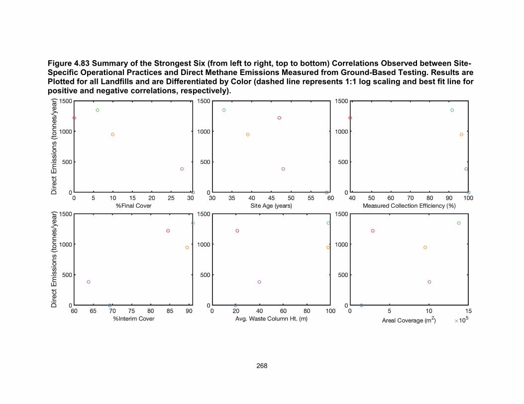
The correlations for total LFG (without CO2 and CO) were controlled by methane and were essentially the same as the data for methane emissions. For total LFG with all four GHGs, the highest correlations were positive and with areal coverage, waste throughput, and waste column height and modest correlations were with WIP, waste depth, site age, precipitation, and modeled collection efficiency. Active face area was moderately correlated to aerial methane and total LFG (with CO2 and CO) emissions. Both aerial methane and total LFG (with CO2 and CO) emissions were moderately positively correlated to LFG collected. Measured waste column height was the only parameter that was strongly correlated to all emissions. Graphical representations for the strongly correlated parameters are provided in Figures 4.82 and 4.83. Aerial methane measurements were mainly sensitive to landfill size characteristics. These measurements did not correlate to specific cover characteristics, climatic conditions, gas collection efficiencies, or landfill organics content or age. Ground methane measurements were strongly correlated to extent of individual cover categories and also correlated to collection efficiencies. These measurements were not highly sensitive to landfill size and climatic conditions. Total LFG emissions were mainly correlated to size parameters and somewhat correlated to collection efficiency. The active face size moderately affected aerial and total LFG emissions. Table 4.20 – Summary of Correlations between Site-Specific Operational Conditions and Direct Emissions of Methane and Total LFG

Landfill Characteristics and

Operational Conditions

Spearman’s Correlation

Coefficient (ρ) for Methane [Aerial, 15

sites]

Spearman’s Correlation

Coefficient (ρ) for Methane [Ground, 5

sites]

Spearman’s Correlation

Coefficient (ρ) for Total LFG [Ground, 5

sites] With

CO2/CO Without CO2/CO

WIP (tonnes) 0.838 0.100 0.700 0.100 Waste Depth (m) 0.732 0.200 0.600 0.200

Waste Throughput (tonnes/day) 0.794 0.300 0.900 0.300

Areal Coverage (m2) 0.753 0.600 1.000 0.600 B0 (%) -0.141 -0.600 -0.200 -0.600

Site Age (years) -0.202 -0.900 -0.700 -0.900 % Daily Cover -0.100 0.500 0.300 0.500

% Interim Cover 0.291 0.800 0.400 0.800 % Final Cover -0.350 -0.900 -0.300 -0.900

Active Face (m2) 0.674 0.200 0.600 0.200 Net Precipitation (mm) -0.018 0.051 0.564 0.051

Average Daily Temperature

(°C) 0.229 0.300 0.500 0.300

LFG Collected (m3) 0.697 -0.200 0.600 -0.200 LFG Flow Rate (m3/min) 0.394 -0.100 0.500 -0.100

266

Landfill Characteristics and

Operational Conditions

Spearman’s Correlation

Coefficient (ρ) for Methane [Aerial, 15

sites]

Spearman’s Correlation

Coefficient (ρ) for Methane [Ground, 5

sites]

Spearman’s Correlation

Coefficient (ρ) for Total LFG [Ground, 5

sites] With

CO2/CO Without CO2/CO

Measured Collection Efficiency (%) -0.212 -0.900 -0.300 -0.900

Modeled Collection Efficiency – Default

Parameters (%) -0.103 -0.200 0.600 -0.200

Modeled Collection Efficiency – Refined

Parameters (%) 0.067 -0.600 0.200 -0.600

Average Measured Waste Age (years) 0.300 0.500 -0.100 0.500

Average Measured Waste Column Height

(m) 1.000 0.700 0.900 0.700

267

Figure 4.82 Summary of the Strongest Six (from left to right, top to bottom) Correlations Observed between Site-Specific Operational Practices and Direct Methane Emissions Measured from Aerial Testing. Results are Plotted for all Landfills and are Differentiated by Color (dashed line represents 1:1 log scaling and best fit line for positive and negative correlations, respectively).

268

Figure 4.83 Summary of the Strongest Six (from left to right, top to bottom) Correlations Observed between Site-Specific Operational Practices and Direct Methane Emissions Measured from Ground-Based Testing. Results are Plotted for all Landfills and are Differentiated by Color (dashed line represents 1:1 log scaling and best fit line for positive and negative correlations, respectively).

269

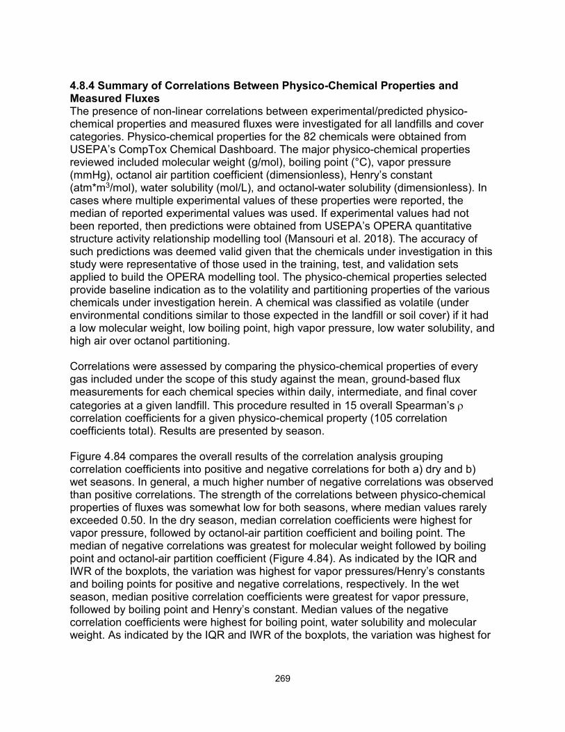
4.8.4 Summary of Correlations Between Physico-Chemical Properties and Measured Fluxes The presence of non-linear correlations between experimental/predicted physico-chemical properties and measured fluxes were investigated for all landfills and cover categories. Physico-chemical properties for the 82 chemicals were obtained from USEPA’s CompTox Chemical Dashboard. The major physico-chemical properties reviewed included molecular weight (g/mol), boiling point (°C), vapor pressure (mmHg), octanol air partition coefficient (dimensionless), Henry’s constant (atm*m3/mol), water solubility (mol/L), and octanol-water solubility (dimensionless). In cases where multiple experimental values of these properties were reported, the median of reported experimental values was used. If experimental values had not been reported, then predictions were obtained from USEPA’s OPERA quantitative structure activity relationship modelling tool (Mansouri et al. 2018). The accuracy of such predictions was deemed valid given that the chemicals under investigation in this study were representative of those used in the training, test, and validation sets applied to build the OPERA modelling tool. The physico-chemical properties selected provide baseline indication as to the volatility and partitioning properties of the various chemicals under investigation herein. A chemical was classified as volatile (under environmental conditions similar to those expected in the landfill or soil cover) if it had a low molecular weight, low boiling point, high vapor pressure, low water solubility, and high air over octanol partitioning. Correlations were assessed by comparing the physico-chemical properties of every gas included under the scope of this study against the mean, ground-based flux measurements for each chemical species within daily, intermediate, and final cover categories at a given landfill. This procedure resulted in 15 overall Spearman’s ρ correlation coefficients for a given physico-chemical property (105 correlation coefficients total). Results are presented by season. Figure 4.84 compares the overall results of the correlation analysis grouping correlation coefficients into positive and negative correlations for both a) dry and b) wet seasons. In general, a much higher number of negative correlations was observed than positive correlations. The strength of the correlations between physico-chemical properties of fluxes was somewhat low for both seasons, where median values rarely exceeded 0.50. In the dry season, median correlation coefficients were highest for vapor pressure, followed by octanol-air partition coefficient and boiling point. The median of negative correlations was greatest for molecular weight followed by boiling point and octanol-air partition coefficient (Figure 4.84). As indicated by the IQR and IWR of the boxplots, the variation was highest for vapor pressures/Henry’s constants and boiling points for positive and negative correlations, respectively. In the wet season, median positive correlation coefficients were greatest for vapor pressure, followed by boiling point and Henry’s constant. Median values of the negative correlation coefficients were highest for boiling point, water solubility and molecular weight. As indicated by the IQR and IWR of the boxplots, the variation was highest for

270

Henry’s constants and boiling points for positive and negative correlations, respectively (Figure 4.84). Figure 4.84 Distributions of Spearman’s ρ (both positive and negative correlations) Describing Correlations between Physico-Chemical Properties and Measured Fluxes for the a) Dry and b) Wet Seasons across all Landfill Sites and Cover Categories.

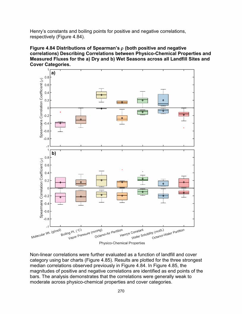
Non-linear correlations were further evaluated as a function of landfill and cover category using bar charts (Figure 4.85). Results are plotted for the three strongest median correlations observed previously in Figure 4.84. In Figure 4.85, the magnitudes of positive and negative correlations are identified as end points of the bars. The analysis demonstrates that the correlations were generally weak to moderate across physico-chemical properties and cover categories.

271

Figures 4.86 and 4.87 further examine the strongest positive and negative correlations observed between physical-chemical properties and measured flux. Qualitatively, the negative correlations were much more apparent than the positive correlations for both seasons, as there was a sharp decrease in molecular weight, boiling point, water solubility, and octanol-air partition coefficients as gas flux decreased (Figure 4.87b). Figure 4.85 Mean Values of Spearman’s ρ (both positive and negative correlations) Describing Correlations between Physico-Chemical Properties and Measured Fluxes for the a) Dry and b) Wet Seasons as a Function of Cover Category. The X-axis Labels Indicate which Physico-Chemical Property and Flux Correlation is Plotted (positive Correlations/negative Correlations).

272

Figure 4.86 Summary of the Three Strongest (from left to right) a) Positive and b) Negative Correlations Observed between Flux and Physical-Chemical Properties in the Dry Season. Results are Plotted for all Chemical Species for a Given Cover Category and Landfill (Gas flux, vapor pressure, and water solubility are scaled logarithmically).

273

Figure 4.87 Summary of the Three Strongest (from left to right) a) Positive and b) Negative Correlations Observed between Flux and Physical-Chemical Properties in the Wet Season. Results are Plotted for all Chemical Species for a Given Cover Category and Landfill (Gas flux, vapor pressure, and water solubility are scaled logarithmically).

274

4.9 Methane Generation and Collection Efficiency Results The results of the LandGEM simulations to predict methane generation rates using both the baseline and refined parameter settings and estimated methane collection efficiencies across landfills is presented in this section of the report. First, the backward and forward prediction of the waste generation trends used as input to the LandGEM model is reviewed (4.9.1). Next, the parameter ranges of L0 and k predicted by the Monte Carlo simulations and ANN model are summarized in Sections 4.9.2 and 4.9.3, respectively. Comparison of methane generation and collection efficiency using both methods and for all landfills is presented in Section 4.9.4. Lastly, a methane mass balance for all landfills is presented in Section 4.9.5 to compare the agreement between methane collection, emission, and generation data. 4.9.1 Back and Forward Fitting of Waste Generation Trends Backward and forward trends in WIP were modeled successfully using a combination of second order polynomials (Poly-1) and two parameter power functions (Power-1) (Figure 4.88 and Table 4.18). Using these mathematical models, acceptable fits could not be obtained for Santa Maria Regional, Salton City, and Sunshine Canyon Landfills. Thus, a simple linear interpolation was used to generate the backward and forward trends in WIP for these two sites. The coefficient of determination (R2) values were greater than 0.97 for the best fitting models (Table 4.18). The magnitude of the scale dependent RMSE was relatively high for all model fits given that the WIP amounts for each site were large (on the order of 104 to 107 tons) across all landfill sites. The best model-data fits generally were obtained for large landfill sites including Bowerman, Redwood, and Yolo County Landfills, indicating the WIP and corresponding waste generation rates were relatively constant over time (Figure 4.88). Increasing WIP and corresponding waste generation rates were obtained for the landfills where the 2nd order polynomial model fits were best (Teapot Dome, Potrero Hills, Chiquita Canyon, and Simi Valley Landfills), whereas waste generation rates were generally decreasing for landfills where the power model fits were best, as the WIP was observed to tail off over time (i.e., Stonyford, Pumice, Borrego, and Site A Landfills). Some landfill sites, including Sunshine Canyon and Salton City were associated with near constant followed by exponentially increasing WIP trends, indicative of alternative periods of low and high waste throughputs. The mathematical models applied avoided over or under-estimating both past and future trends in WIP; therefore, the corresponding waste generation rates for these past and future time periods were deemed acceptable as input for the LandGEM simulations.

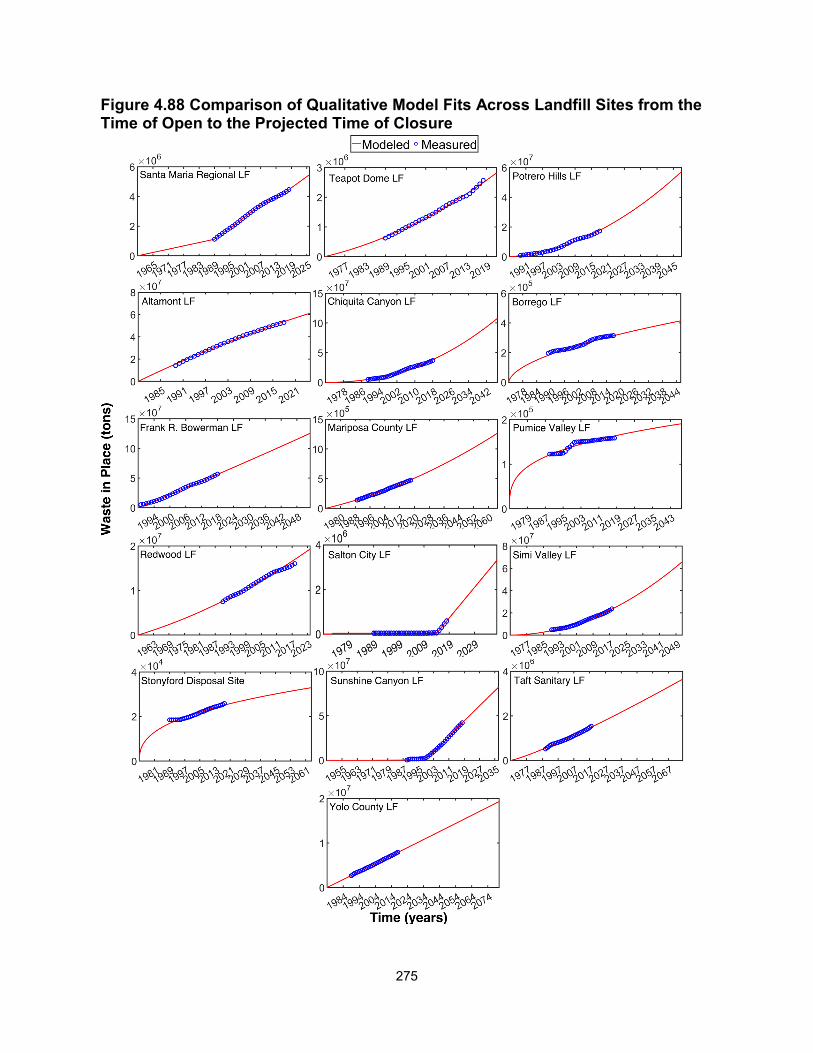
275

Figure 4.88 Comparison of Qualitative Model Fits Across Landfill Sites from the Time of Open to the Projected Time of Closure

276

Table 4.21 – Quantitative Model Fitting Metrics for Each Landfill Site Landfill Best Fitting Model R2 RMSE

Santa Maria Regional Landfill Linear-Interpolation N/A N/A

Teapot Dome Polynomial-1 0.999 2.46E+04 Potrero Hills Polynomial-1 0.992 4.93E+05

Altamont Landfill Polynomial-1 0.999 4.24E+05 Chiquita Canyon Power-1 0.988 1.78E+06 Borrego Landfill Power-1 0.988 6.90E+03

Frank R. Bowerman Polynomial-1 0.996 1.10E+06 Mariposa County LF Polynomial-1 0.999 3.84E+03

Pumice Valley LF Power-1 0.979 4.29E+03 Redwood LF Polynomial-2 0.999 5.56E+07

Salton City LF Linear-Interpolation N/A N/A Simi Valley Polynomial-1 0.999 2.72E+05

Stonyford Disposal Site Power-1 0.971 1.03E+03 Sunshine Canyon Linear-Interpolation N/A N/A

Taft Sanitary Landfill Power-1 0.991 4.56E+04 Yolo County Landfill Polynomial-1 0.999 3.07E+04

N/A Not applicable since linear interpolation was used

4.9.2 Monte Carlo Simulations: L0 Results The Monte Carlo simulations used to predict L0 values were highly influenced by the landfill specific waste compositions (i.e., weighting factors) obtained from extrapolated data sources (CalRecycle 2019). The outputs predictions were likely more sensitive to the weighting factor inputs given that these values were not allowed to vary in the MC simulations. The differences in the input weighting factors as a function of landfill site are provided in Table 4.19. Food waste comprised a majority of the residential and commercial biodegradable MSW waste streams for all sites, ranging from 35-52% of the total biodegradable waste disposed. Despite recent diversion strategies and legislation, food waste has and continues to be a significant fraction of the total biodegradable component of MSW in California landfills (California SB 1383). In addition, this waste component was generally highest as it also incorporated the remaining unclassified portion of biodegradable organics, which could not be classified into another material type under the “other organic” material category in the CalRecylce waste characterization data. The next most significant waste components were identified as miscellaneous paper (ranging from 21-24%), mixed yard waste (ranging from 6-18%), as well as mixed wood waste (ranging from 6-14%) (Table 4.19). All other waste component categories, including mixed textile wastes, were generally below 6% of the total biodegradable waste disposed for the landfills included in the study. Of the major waste components identified above, Potrero Hills, Sunshine Canyon, Redwood, and Frank Bowerman Landfills had the largest fractions of food waste, miscellaneous paper wastes, yard wastes, and wood wastes disposed, respectively. The variation in

277

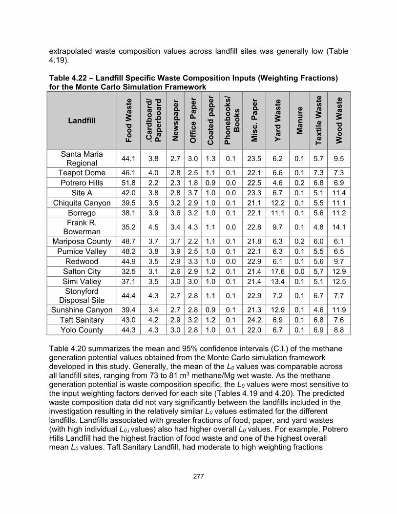
extrapolated waste composition values across landfill sites was generally low (Table 4.19). Table 4.22 – Landfill Specific Waste Composition Inputs (Weighting Fractions) for the Monte Carlo Simulation Framework

Landfill Fo

od W

aste

.Car

dboa

rd/

Pape

rboa

rd

New

spap

er

Offi

ce P

aper

Coa

ted

pape

r

Phon

eboo

ks/

Boo

ks

Mis

c. P

aper

Yard

Was

te

Man

ure

Text

ile W

aste

Woo

d W

aste

Santa Maria Regional 44.1 3.8 2.7 3.0 1.3 0.1 23.5 6.2 0.1 5.7 9.5

Teapot Dome 46.1 4.0 2.8 2.5 1.1 0.1 22.1 6.6 0.1 7.3 7.3 Potrero Hills 51.8 2.2 2.3 1.8 0.9 0.0 22.5 4.6 0.2 6.8 6.9

Site A 42.0 3.8 2.8 3.7 1.0 0.0 23.3 6.7 0.1 5.1 11.4 Chiquita Canyon 39.5 3.5 3.2 2.9 1.0 0.1 21.1 12.2 0.1 5.5 11.1

Borrego 38.1 3.9 3.6 3.2 1.0 0.1 22.1 11.1 0.1 5.6 11.2 Frank R.

Bowerman 35.2 4.5 3.4 4.3 1.1 0.0 22.8 9.7 0.1 4.8 14.1

Mariposa County 48.7 3.7 3.7 2.2 1.1 0.1 21.8 6.3 0.2 6.0 6.1 Pumice Valley 48.2 3.8 3.9 2.5 1.0 0.1 22.1 6.3 0.1 5.5 6.5

Redwood 44.9 3.5 2.9 3.3 1.0 0.0 22.9 6.1 0.1 5.6 9.7 Salton City 32.5 3.1 2.6 2.9 1.2 0.1 21.4 17.6 0.0 5.7 12.9 Simi Valley 37.1 3.5 3.0 3.0 1.0 0.1 21.4 13.4 0.1 5.1 12.5 Stonyford

Disposal Site 44.4 4.3 2.7 2.8 1.1 0.1 22.9 7.2 0.1 6.7 7.7

Sunshine Canyon 39.4 3.4 2.7 2.8 0.9 0.1 21.3 12.9 0.1 4.6 11.9 Taft Sanitary 43.0 4.2 2.9 3.2 1.2 0.1 24.2 6.9 0.1 6.8 7.6 Yolo County 44.3 4.3 3.0 2.8 1.0 0.1 22.0 6.7 0.1 6.9 8.8

Table 4.20 summarizes the mean and 95% confidence intervals (C.I.) of the methane generation potential values obtained from the Monte Carlo simulation framework developed in this study. Generally, the mean of the L0 values was comparable across all landfill sites, ranging from 73 to 81 m3 methane/Mg wet waste. As the methane generation potential is waste composition specific, the L0 values were most sensitive to the input weighting factors derived for each site (Tables 4.19 and 4.20). The predicted waste composition data did not vary significantly between the landfills included in the investigation resulting in the relatively similar L0 values estimated for the different landfills. Landfills associated with greater fractions of food, paper, and yard wastes (with high individual L0,i values) also had higher overall L0 values. For example, Potrero Hills Landfill had the highest fraction of food waste and one of the highest overall mean L0 values. Taft Sanitary Landfill, had moderate to high weighting fractions

278

observed for all waste components, which also resulted in a high predicted L0 (Table 4.20). While the variation of L0 between the landfill sites was not significant, the results of the Monte Carlo simulations indicated a high variation in predicted methane generation potentials for a given landfill (Table 4.20). The high variation in predicted L0 values was a factor of the high uncertainty of the waste component specific methane generation potentials (L0,i) obtained from the literature. Reported values of waste component specific L0,i varied significantly given that the studies from which the L0,i values were derived included different waste materials or mixtures of waste materials in the laboratory scale BMP assays. Moreover, many of these studies did not use consistent BMP protocols (Buffiere et al. 2006, Machado et al. 2009, Krause et al. 2018b). However, the 95% confidence intervals are generally within the range of acceptable values as defined by the USEPA (6.2 to 270 m3/Mg wet waste), demonstrating that the MC simulations captured the full range in uncertainty of the model inputs. Table 4.23 – L0 Values Predicted using the Monte Carlo Simulation Framework Developed in this Study

Landfill Mean L0 Value (m3/Mg wet waste) 95% C.I.

Santa Maria Regional 78.8 [8.61, 302] Teapot Dome 79.7 [8.62, 308] Potrero Hills 80.3 [8.30, 319]

Site A 77.6 [8.53, 296] Chiquita Canyon 76.6 [8.73,286] Borrego Landfill 76.9 [8.98, 283]

Frank R. Bowerman 76.2 [9.07, 278] Mariposa County 79.9 [8.46, 313]

Pumice Valley 79.6 [8.40, 312] Redwood 78.5 [8.55, 302]

Salton City 73.5 [8.66, 269] Simi Valley 74.2 [8.42, 278]

Stonyford Disposal Site 79.8 [8.77, 305] Sunshine Canyon 75.4 [8.47, 284]

Taft Sanitary 81.3 [9.21, 305] Yolo County 78.3 [8.47, 302]

4.9.3 Artificial Neural Network Predictions: k Results Results obtained from the novel, global optimization procedure developed herein indicated that an artificial neural network architecture with three layers (input, 1 hidden layer, output) was sufficient for accurately predicting first-order decay rate values (Table 4.22). From this optimization routine, a total of four neurons within the hidden layer was deemed optimal. The overall predictive performance (sum of the training, testing, and validation performance) of the optimized ANN was excellent, given the

279

quantitative metrics of goodness of fit summarized in Table 4.22. The MSE and normalized MSE (NMSE) values of the ANN ranged were low and comparable across all divisions of the datasets used. Similarly, the coefficient of determination values were high (0.84-0.903), indicating that the ANN was properly trained and capable of making accurate and reliable predictions of unobserved data. The similarity of the predictive performance metrics (and high validation scores) suggests that the ANN did not overfit the training and/or testing datasets and that proper regularization was carried out during training/optimization of the neural network architecture. Regularization was ensured by explicitly normalizing the MSE values from all datasets by the overall expected variance of the model predictions. Table 4.24 – Predictive Performance of the Optimized ANN Architecture

Dataset MSE NMSE R2

Overall 0.000603 0.111 0.889 Training 0.000653 0.111 0.889 Testing 0.000404 0.157 0.843

Validation 0.000573 0.097 0.903

The qualitative fitting performance of the ANN across the different divisions of the dataset is presented in Figure 4.89, where the observed k values are plotted against the predicted k values by the ANN. A 1:1 line is provided for reference, which delineates a perfect agreement between the observed and predicted k values. An empirical 95% prediction interval was determined using a quasi-MC approach by running the ANN model a large number of times (N = 1,000,000) across the full range in the input space (using a Sobol sequence for each input). In this approach, observed values were estimated from the predicted values assuming that the errors were normally distributed with mean 0 and standard deviation equal to the square root of the MSE values. Most of the data points are clustered close to the 1:1 line, indicating good overall agreement between the observed and predicted k-values (Figure 4.89). Only a few data points lie outside the 95% prediction interval, confirming that the ANN model could successfully predict k values within an acceptable degree of certainty using the eight distinct inputs of the dataset developed. Several predictions on the unobserved data (validation dataset) lie right on the 1:1 reference line, further confirming that the ANN model can generalize well and was not subject to overfitting during the training process (Figure 4.89). Similar observations can be made regarding the qualitative fitting results of the test set as compared to the validation set.

280

Figure 4.89 Qualitative Evaluation of ANN Predictive Performance for Overall, Training, Testing, and Validation Datasets.

A summary of the input values used to generate k-value predictions is presented in Table 4.22. The WIP values were estimated based on the procedure described in Section 3.8, whereas the throughput, depth, and area were used directly from the most recent estimates provided by the landfills included in the investigation. Normal annual precipitation and average daily temperatures were determined from the most recent 30-year data compiled by the NOAA using the closest weather stations available to each landfill. The total biodegradable waste fraction (B0) was determined using the data extrapolated from the CalRecycle database and included estimation of site specific L0 values (total disposed amount of biodegradable waste normalized by the total disposed waste). Relative waste age was defined as the time period spanning from the start of landfill operations (i.e., active waste placement) to 2019. In addition to B0 values and relative waste ages, the input factors varied significantly as a function of landfill site. Pumice Valley and Sunshine Canyon landfills were the coldest and warmest sites, respectively. Many sites were located in temperate climate zones (avg. daily temperatures ranging from 16-19°C) differentiated by rainfall received, including Teapot Dome, Potrero Hills, Site A, Chiquita Canyon, Frank R. Bowerman, Simi Valley, Sunshine Canyon, Taft Sanitary, and Yolo County landfills (Table 4.22). Redwood and Salton City landfills received the highest and lowest rainfall per year. Rainfall rates at the landfills in the temperate climates varied from 278 to 630 mm/year. Across all landfills, WIP and landfill area varied by four and three orders of magnitude, respectively. Throughput rates and waste depths generally paralleled trends in WIP/area, as indicated by data presented in Table 4.22.

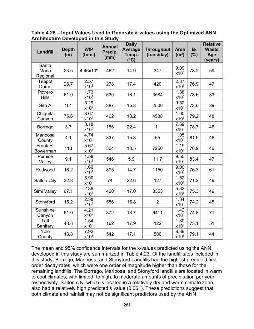
281

Table 4.25 – Input Values Used to Generate k-values using the Optimized ANN Architecture Developed in this Study

Landfill Depth (m)

WIP (tons)

Annual Precip. (mm)

Daily Average Temp.

(°C)

Throughput (tons/day)

Area (m2)

B0 (%)

Relative Waste Age

(years) Santa Maria

Regional 23.5 4.46x106 462 14.9 347 9.09

x105 78.2 59

Teapot Dome 28.7 2.57

x106 278 17.4 420 2.87 x105 76.9 47

Potrero Hills 61.0 1.73

x107 630 16.1 3584 1.38 x106 73.6 33

Site A 101 5.29 x107 387 15.8 2500 9.52

x105 73.6 39

Chiquita Canyon 75.6 3.67

x107 462 18.2 4588 1.00 x106 79.2 48

Borrego 3.7 3.18 x105 156 22.4 11 7.69

x104 78.7 46

Mariposa County 4.1 4.74

x105 837 15.3 65 1.05 x105 81.9 46

Frank R. Bowerman 113 5.67

x107 364 18.5 7250 1.19 x106 76.9 46

Pumice Valley 9.1 1.58

x105 546 5.9 11.7 9.55 x104 83.4 47

Redwood 16.2 1.60 x107 895 14.7 1150 9.00

x105 76.3 61

Salton City 32.8 5.90 x105 74 22.6 127 1.62

x104 71.2 49

Simi Valley 67.1 2.36 x107 420 17.0 3353 5.82

x105 75.3 49

Stonyford 15.2 2.58 x104 586 15.8 2 1.34

x104 74.2 45

Sunshine Canyon 61.0 4.21

x107 372 18.7 6411 1.42 x106 74.8 71

Taft Sanitary 48.8 1.54

x106 162 17.9 122 1.80 x105 73.1 51

Yolo County 18.8 7.92

x106 542 17.1 500 8.39 x105 79.1 44

The mean and 95% confidence intervals for the k-values predicted using the ANN developed in this study are summarized in Table 4.23. Of the landfill sites included in this study, Borrego, Mariposa, and Stonyford Landfills had the highest predicted first order decay rates, which were one order of magnitude higher than those for the remaining landfills. The Borrego, Mariposa, and Stonyford landfills are located in warm to cool climates, with limited, to high, to moderate amounts of precipitation per year, respectively. Salton city, which is located in a relatively dry and warm climate zone, also had a relatively high predicted k value (0.061). These predictions suggest that both climate and rainfall may not be significant predictors used by the ANN

282

architecture. Rainfall was more influential than temperature in the ANN model as Mariposa Landfill had a high predicted k value. Generally, previous studies have indicated that greater moisture contents, influenced by rainfall received, and higher temperatures are associated with higher k values. Other site-specific operational characteristics such as WIP/areal coverage, waste age, and available organic fraction of waste components in the waste mass also were determined to be significant for making reliable predictions. As compared to predicted L0 values, the 95% confidence intervals obtained for the ANN predictions were more constrained. This result may be due to several factors, including the fact that k values reported in the literature do not span a wide range (i.e., two orders of magnitude, excluding bioreactor landfills) and that the ANN predictions are highly accurate (MSE values below 0.1). Given that the residuals in the loss function were assumed to be Gaussian, white noise, the resulting variation in predicted values was expected to be small. Table 4.26 – k Values Predicted Using the ANN Architecture Optimized in this Study

Landfill Mean k Value (1/year) 95% C.I.

Santa Maria Regional 0.0594 [0.0523, 0.0660] Teapot Dome 0.0287 [0.0221, 0.0353] Potrero Hills 0.0928 [0.0862, 0.0994]

Site A 0.0210 [0.0154, 0.0286] Chiquita Canyon 0.0330 [0.0265,0.0397]

Borrego 0.226 [0.219, 0.232] Frank R. Bowerman 0.0134 [0.00680, 0.0200]

Mariposa County 0.224 [0.217, 0.230] Pumice Valley 0.0359 [0.0290, 0.0425]

Redwood 0.0741 [0.0674, 0.0807] Salton City 0.0610 [0.0539, 0.0672] Simi Valley 0.0152 [0.00855, 0.0218] Stonyford 0.119 [0.113, 0.126]

Sunshine Canyon 0.0624 [0.0558, 0.0690] Taft Sanitary 0.00771 [0.00110, 0.0143] Yolo County 0.0556 [0.0490, 0.0622]

To evaluate the differences between regression models developed by previous studies to the more advanced architecture herein, several additional factors were investigated. In particular, presence or absence of correlation among inputs, presence or absence of correlation between inputs and targets, and input sensitivity on ANN predictive accuracy were studied. In general, ANN predictions are affected by input correlation, with low predictive significance when input variables are highly correlated to one another. Input variables that are highly correlated with output targets are of high

283

importance when developing the ANN architecture. Input sensitivity encompasses both factors, indicating how influential the input variables are when the ANN model generates predictions. Both input-input and input-target (output) correlations were assessed using Spearman’s non-linear correlation coefficient, ρ. Input sensitivity was evaluated by setting the input variable to zero (keeping all other inputs constant, non-zero values – the modified approach), and calculating the RMSE between the MSE of the non-modified input matrix to that obtained from the modified input matrix (Δ). All of these factors were investigated using the full dataset, including training, testing, and validation data. Correlations among input variables in the dataset are compared visually in the heatmap presented in Figure 4.90. For correlation among inputs, significant (i.e., ρ > 0.5), positive non-linear correlations were observed between all operational factors, including WIP and depth, WIP and area, and WIP and throughput, with ρ values ranging from 0.5 to 0.75. There was a moderate (0.3<ρ<0.5), positive correlation between annual precipitation and daily average temperature (0.40) and moderate, negative correlations between annual precipitation and waste age and biodegradable fraction of waste components (-0.40 to -0.43). Significant, positive correlations were observed between waste age and depth, WIP, and areal coverage, with ρ ranging from 0.47 to 0.52 (Figure 4.90).The average, absolute ρ values were lowest for B0 and daily average temperature, suggesting that these inputs were more favorable for making accurate predictions from the ANN model. Figure 4.90 Correlation Between Input Variables of the Dataset Used for Training, Testing, and Validating the ANN Model (down arrows: negative correlations; color: strength of correlation, where red = strong and blue = weak).

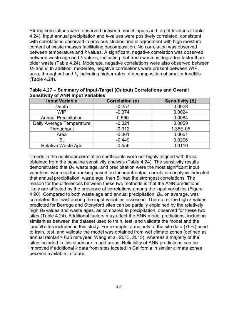
284

Strong correlations were observed between model inputs and target k values (Table 4.24). Input annual precipitation and k-values were positively correlated, consistent with correlations observed in previous studies and in agreement with high moisture content of waste masses facilitating decomposition. No correlation was observed between temperature and k values. A significant, negative correlation was observed between waste age and k values, indicating that fresh waste is degraded faster than older waste (Table 4.24). Moderate, negative correlations were also observed between B0 and k. In addition, moderate, negative correlations were present between WIP, area, throughput and k, indicating higher rates of decomposition at smaller landfills (Table 4.24). Table 4.27 – Summary of Input-Target (Output) Correlations and Overall Sensitivity of ANN Input Variables

Input Variable Correlation (ρ) Sensitivity (Δ) Depth -0.257 0.0028 WIP -0.374 0.0024

Annual Precipitation 0.560 0.0084 Daily Average Temperature -0.021 0.0059

Throughput -0.312 1.35E-05 Area -0.361 0.0061 B0 -0.449 0.0206

Relative Waste Age -0.556 0.0110 Trends in the nonlinear correlation coefficients were not highly aligned with those obtained from the baseline sensitivity analysis (Table 4.24). The sensitivity results demonstrated that B0, waste age, and precipitation were the most significant input variables, whereas the ranking based on the input-output correlation analysis indicated that annual precipitation, waste age, then B0 had the strongest correlations. The reason for the differences between these two methods is that the ANN predictions likely are affected by the presence of correlations among the input variables (Figure 4.90). Compared to both waste age and annual precipitation, B0, on average, was correlated the least among the input variables assessed. Therefore, the high k values predicted for Borrego and Stonyford sites can be partially explained by the relatively high B0 values and waste ages, as compared to precipitation, observed for these two sites (Table 4.24). Additional factors may affect the ANN model predictions, including similarities between the dataset used to train, test, and validate the model and the landfill sites included in this study. For example, a majority of the site data (75%) used to train, test, and validate the model was obtained from wet climate zones (defined as annual rainfall > 635 mm/year, Wang et al. 2013, 2015), whereas a majority of the sites included in this study are in arid areas. Reliability of ANN predictions can be improved if additional k data from sites located in California in similar climate zones become available in future.

285

4.9.4 Methane Generation and Gas Collection Efficiency: Baseline and Refined LandGEM Predictions Annual methane generation rates estimated using LandGEM with the L0 and k parameters from the baseline and refined approaches are presented in Figure 4.91. The trends in methane generation rates over time were in general similar between the two approaches and were affected by trends in estimated waste placement data in both cases. Pronounced peaks in methane production is followed by a quick decline in generation for landfills with high WIP. Landfills with smaller WIP demonstrated a slow increase to peak methane generation followed by a prolonged tail in methane generation beyond site closure. In the baseline approach, for landfills with high WIP, the order of methane generation from highest to lowest was for Chiquita Canyon, Frank R. Bowerman, Sunshine Canyon, Simi Valley, Site A, and Potrero Hills Landfills (Figure 4.91a). This order was modified to Sunshine Canyon, Chiquita Canyon, Potrero Hills, Frank R. Bowerman, Site A, and Simi Valley with the refined approach (Figure 4.91b). The variations in methane generation over time was somewhat more gradual for the refined analysis compared to the baseline analysis. The LandGEM predictions for annual methane generation rates using the baseline parameter values were higher than the predictions obtained using the refined approach (2x108 compared to 1.5x108 m3/year). Default methane generation potential values were on the order of 100 to 170 m3/Mg wet waste, as compared to 70-80 m3/Mg wet waste used in the refined approach. The higher methane generation potentials in the default LandGEM simulations resulted in the higher rates of methane generation (Figure 4.91). Default first order decay rate values were 0.02, 0.04, or 0.05 year-1, whereas refined estimates of k varied by site and ranged from 0.007 to 0.22 year-1. The greater variation in the k values in the refined analysis mainly controlled the slopes of the methane generation-time relationships resulting in generally in character with yet more varied slopes compared to the baseline analysis.

286

Figure 4.91 LandGEM Methane Generation Rates a) Baseline, b) Refined Approach.

A detailed summary of estimated gas collection efficiencies (for the year 2018, mean and 95% confidence intervals) for both the measured and modeled (baseline and refined) LandGEM approaches is presented in Table 4.26. Mean values of the measured collection efficiencies were generally high, ranging from 38.9 to 99.8%

287

across landfills. Santa Maria Regional and Teapot Dome Landfills had the highest and lowest measured collection efficiencies, respectively. In addition, the corresponding variation in measured methane collection efficiencies was relatively low, as indicated by the constrained 95% confidence intervals presented in Table 4.26. For modeled methane generation using the baseline approach, the collection efficiencies ranged from 25 to 76% and were highest and lowest for the Redwood and Teapot Dome Landfills, respectively. For modeled methane generation using the refined approach, collection efficiencies ranged from 37.4 to 100% and were highest for the Frank Bowerman, Redwood, and Simi Valley Landfills. In line with the baseline results, Teapot Dome had the lowest methane collection efficiency using the refined approach. The mean 𝛼𝛼 values obtained from the refined approach exceeded 100% for the Frank Bowerman, Redwood, and Simi Valley Landfills. As collection efficiencies higher than 100% are unrealistic; efficiencies were reported as 100% for these sites. Application of the lower 95% range in the parameter estimates for the refined approach generally resulted in an underapproximation of methane generation, and hence collection efficiencies exceeding 100%, even though these were based on realistic values using the full range in uncertainty expected for each prediction method. In general, collection efficiencies were higher using the refined estimates of the parameters compared to the default parameter values. Higher methane generation rates were predicted using the baseline approach as compared to the refined approach resulting in the lower collection efficiencies associated with the baseline approach. The variation in methane collection efficiencies was generally lower for the baseline approach, as indicated by the narrow 95% confidence intervals. The variation in collection efficiencies was higher for the refined approach due to the high uncertainty in the overall methane generation potential for each site, which ranged from 8 to 319 m3/Mg wet waste (Table 4.20).

288

Table 4.28 – Summary of Measured and Modeled Methane Gas Collection Efficiencies using the Baseline and Refined LandGEM Parameter Values (for year 2018)

Landfill Measured-Aerial Data

Measured-Ground Data Baseline Refined

𝜶𝜶� (%) 95% C.I. 𝜶𝜶�

(%) 95% C.I. 𝜶𝜶� (%) 95% C.I. 𝜶𝜶�

(%) 95% C.I.

Santa Maria Regional 61.1 [42,

100] 100 [100, 100] 51.5 [31.9,

82.8] 60.3 [15.4, 100*]

Teapot Dome 23.2 [18.4, 31.4] 38.9 [30.3,

54.4] 24.5 [14.7, 38.9] 37.4 [8.8,

100*]

Potrero Hills 47.3 [43.2, 52.3] 91.4 [88.9, 94] 60.2 [34,

93.5] 49.7 [12.3, 100*]

Site A 62.9 [57.7, 69.0] 96.4 [93.9,

98.9] 39.6 [24.6, 63.8] 72 [16.6,

100*]

Chiquita Canyon 84.1 [80.8, 87.7] 98.8 [98.3,

99.3] 62.5 [36.4, 98.2] 90.9 [22.3,

100*]

Frank R. Bowerman 58.7 [54.1, 64.1] N/A N/A 53 [30.8,

83.2] 100* [31.2, 100*]

Redwood 91.4 [89.2, 93.8] N/A N/A 75.9 [53.9,

100*] 100* [26.3, 100*]

Simi Valley 78.3 [70.3, 88.5] N/A N/A 65.3 [38.9,

100*] 100* [36.2, 100*]

Sunshine Canyon 86.8 [84.4, 89.4] N/A N/A 63.7 [36.1,

99.1] 62.3 [15.8, 100*]

Yolo County 57.6 [53.4, 62.4] N/A N/A 48 [29.8,

77.2] 57.8 [14.6, 100*]

*Indicates that calculated gas collection efficiency exceeded 100% N/A Not applicable 4.9.5 Methane Mass Balance The results of the methane mass balance analysis that was conducted for each landfill are presented in Table 4.27. For a majority of the landfills, excess methane is present (77 to 18,820 tonnes) that can be attributed to storage, migration, or oxidation pathways. Most of the excess methane can be attributed to oxidation taking place in the covers as storage and migration are less significant components of the methane balance in the landfill environment (Christophersen and Kjeldsen 2001, Scheutz et al. 2009a). In general, landfills with higher WIP were associated with higher methane collection, emission, and excess amounts. Sites without an active gas extraction system in place generally had small to moderate values of methane stored, migrated, or oxidized, ranging from below 0 to 907 tonnes per year. For some of these sites without an extraction system, net uptake was estimated (Table 4.27). For select landfills with gas extraction systems, including Frank R. Bowerman, Redwood, Yolo, and Simi Valley Landfills, there is a net deficit of methane, indicating that the mean LandGEM simulations using the refined parameter sets did not match measured collection or emissions data. This difference in measured and predicted values most likely resulted from inadequate approximations of site and waste specific k and L0 values.

289

The uncertainty in methane flow estimates was generally highest for the LandGEM generation predictions followed by the emissions and collections estimates (Table 4.27). The magnitude of the 95% confidence intervals is high for methane generation (on the order of 104 to 108), which carries over to the high overall uncertainty of the excess/deficit estimates. The uncertainty in LandGEM predictions was high due to the wide range in methane generation potentials predicted from the MC analysis, which are representative of the highly variable waste compositions at the landfills. The uncertainty of the aerial emission measurements was significantly higher than that for the ground-based measurements, based on the magnitude of the 95% confidence intervals in Table 4.27. Gas collection measurement uncertainty was very low, ranging from 0.5 to 2 tonnes of methane as the LFG flow and methane composition were not observed to vary significantly across the datasets obtained and analyzed from previous studies.

290

Table 4.29 – Summary of Methane Mass Balance Results (the mean and 95% confidence intervals are presented in the first and second rows, respectively)

Landfill CH4

Generated (tonnes)

CH4 Collected (tonnes)

CH4 Emitted (tonnes)

ΔCH4 Excess/Deficita

(tonnes) Santa Maria

Regional 4379 2640 -0.1221 1738.8

±1.27x107 ±0.536 ±0.079 ±1.27x107

Teapot Dome 2074 777 1220 77.2 ±6.57x106 ±0.313 ±571 ±6.57x106

Potrero Hills 29629 14732 1391 13506 ±8.89x107 ±1.14 ±446 ±8.89x107

Site A 34745 25026 945 8774 ±1.12x107 ±1.45 ±446 ±1.12x108

Chiquita Canyon

33878 30784 381 2713 ±1.03x108 ±1.58 ±154 ±1.03x108

Borrego 143 0 36 107 ±3.85x105 0 ±10.5 ±3.85x105

Frank R. Bowerman

27490 40764 28693 -41966 ±9.80x107 ±1.79 ±5856 ±9.80x107

Mariposa County

567 0 79 489 ±1.65x106 0 ±129 ±1.65x106

Pumice Valley 82 0 -2 84 ±2.34x105 0 ±14.9 ±2.34x105

Redwood 12875 13051 1225 -1400 ±3.68x107 ±1.09 ±364 ±3.68x107

Salton City 1002 0 95 907 ±2.94x106 0 ±26.3 ±2.94x106

Simi Valley 11875 20213 5586 -13924 ±4.19x107 ±1.32 ±2954 ±4.19x107

Stonyford 15 0 53 -39 ±4.15x104 0 ±12.3 ±4.15x104

Sunshine Canyon

66618 41504 6294 18820 ±1.95x108 ±1.81 ±1361 ±1.95x108

Taft Sanitary 472 0 -215 687 ±2.04x106 0 ±287 ±2.04x106

Yolo County 7726 4464 3290 -28 ±2.26x107 ±0.676 ±599 ±2.26x107

a Calculated as methane generated minus the sum of methane collected and emitted