Embed Size (px)
Citation preview

478 Advanced Operations Research
Istvan Maros
Department of Computing
Imperial College, London
2008 November 13
Version v3.2d
Advanced OR v3.2d
Introduction 1
Outline
1. Decision making and operations research.
(a) The need for optimization.
(b) Typical models of industry and finance.
2. Advanced linear programming (LP)
(a) Need for linear models.
(b) General form of LP problems.
(c) The sparse simplex method; primal and dual algorithms;
computational implications.
(d) Economic interpretation of the optimality conditions:
Sensitivity analysis.
(e) Interior point algorithms.
(f) State-of-the-art in solving LP problems.
3. Integer programming (IP)
(a) Situations requiring integer valued models.
(b) IP problem formulation.
(c) Solution methods; Implicit enumeration, branch and bound
(B&B) method.
(d) Network programming (optimization in networks).
(e) Logic constraints and IP.
(f) State-of-the-art in solving IP problems.
4. Modeling
(a) Basics of modeling.
(b) Model generation and management.
(c) Modeling languages, modeling systems.
Advanced OR v3.2d 2008/11/13

Introduction 2
Traditional decision support(What–if type modeling)
1. Observing and formulating the problem.
2. Constructing a computational model that captures the essence
of the real problem.
3. Picking (guessing) a solution to the model (also referred to as
generating an alternative).
4. Evaluating the solution and analyzing its validity. Comparing
it with solutions obtained so far (learning).
5. Depending on the outcome of step 4, generating a new
alternative and returning to step 4 or modifying the model and
returning to step 3 or accepting the currently best solution.
6. Presenting the results to decision makers.
Advantages: Gives answers to “what if” type questions, easy
to use, a priori knowledge of model can help generate reasonable
alternatives. Spreadsheets are the typical computational tools for
this type of analysis.
Disadvantages: Process is slow if too many alternatives are
evaluated, search for a good solution is unguided, a “guess”
solution may not even be technically feasible, inaccurate if too
few solutions are tested, the quality of the accepted solution is
unknown (how much better could have been found).
There is a need for optimization.
Advanced OR v3.2d 2008/11/13
Introduction 3
Modern decision supportusing optimization technology
1. Observing and formulating the problem. It usually involves
the use of logic programming methodology that can provide a
natural framework for problem specification.
2. Constructing a computational model that captures the essence
of the real problem.
3. Deriving a solution from the model: Solving the problem using
large scale sparse optimization technology. This results in a
best possible (optimal) solution under the constraints of the
model.
4. Verifying and analyzing the validity of results. If necessary, the
model is modified and the process is resumed at step 3.
5. Presenting the results to decision makers.
This is the area of applying advanced computational tools and
techniques of operations research.
Advanced OR v3.2d 2008/11/13

Introduction 4
Some application areas of advanced OR
The same tools can be used in very different areas like
• Industry (petroleum, chemical, manufacturing, food, steel,
paper)
• Finance
• Telecommunications
• Transport
• Agriculture
• Energy
• Defence
• Mining
• Government
• Healthcare
• Manpower Planning
• Advertising
• etc.
Advanced OR v3.2d 2008/11/13
Introduction 5
Characteristics of real-life decision problems
Real-life decision problems are typically
1. Large: Many variables, equations and constraints are needed
to create realistic models.
2. Complex: Model may include time dependence, feedback
and nonlinearity. Additional features may include logical
relationships among variables and constraints, integrality
requirement of some variables, etc.
3. Sparse: The computational model usually consists of vectors
and matrices of large scale. They are sparse, that is, contain
very few nonzero entries. The ratio of nonzeros to the total
number of positions is often in the range of 0.05%–1.00%.
By using proper computational tools, sparsity enables us to
represent and solve such problems.
4. Difficult to solve, due to their size and complexity. Different
models require completely different solution methods. For each
type of model there exist several solution algorithms. They have
been designed to cope with arising numerical and algorithmic
difficulties.
Advanced OR v3.2d 2008/11/13

Introduction 6
Product Mix(simplified model)
The most typical industrial problem is to determine the optimal
product mix that maximizes revenue (or profit).
A flourishing manufacturing company can produce 6 different
products, Pr-1, . . . , Pr-6. They require labour, energy, and
processing on machines. These resources are available in limited
amounts. The company wants to determine what quantities
to produce that maximize the monthly revenue, assuming that
any amount can be sold. The following table describes the
technological requirements of producing one unit of each product,
the corresponding revenue and the monthly availability of the
resources.
Pr-1 Pr-2 Pr-3 Pr-4 Pr-5 Pr-6 Limit
Revenue 5 6 7 5 6 7
Machine
hour 2 3 2 1 1 3 1050
Labour
hour 2 1 3 1 3 2 1050
Energy 1 2 1 4 1 2 1080
Advanced OR v3.2d 2008/11/13
Introduction 7
The decision variables are the unknown quantities of the products.
They are denoted by x1, . . . , x6.
The revenue to be maximized is
5x1 + 6x2 + 7x3 + 5x4 + 6x5 + 7x6
The resource constraints are:
2x1 + 3x2 + 2x3 + 1x4 + 1x5 + 3x6 ≤ 1050
2x1 + 1x2 + 3x3 + 1x4 + 3x5 + 2x6 ≤ 1050
1x1 + 2x2 + 1x3 + 4x4 + 1x5 + 2x6 ≤ 1080
Since production must be nonnegative, we impose xj ≥ 0, j =
1, . . . , 6.
This is a simple LP problem that can be solved by the simplex
method. The solution is x2 = 240, x4 = 90, x5 = 240, and
x1 = x3 = x6 = 0, giving a revenue of 3330.00 units.
While the problem is simple its analysis highlights some interesting
points.
• The most rewarding products (Prod-3 and Prod-6) are not
included in the optimal mix.
• It is sufficient to produce not more than three products in order
to achieve the maximum possible revenue.
• All resources are fully utilized (constraints are satisfied with
equality).
Advanced OR v3.2d 2008/11/13

Introduction 8
Portfolio Optimization(simplified model)
Investor’s portfolio at the beginning of the year:
Share # of shares held current value
per share
Shiny 75 £20
Risky 1000 £2
Trusty 25 £100
There is a one-off chance to change the portfolio for a whole year
ahead. It is assumed that at the end of the year the position of
the shares will be:
Share dividend value
per share per share
Shiny £5 £18
Risky £0 £3
Trusty £2 £102
Investor does not want to change the composition of the portfolio
but possibly the quantities. It is assumed that there is no fee for
buying or selling stocks and fractional stocks are permitted.
Advanced OR v3.2d 2008/11/13
Introduction 9
Purpose: to adjust the portfolio to maximize the end-of-year
dividends subject to the following restrictions:
1. Current value of the portfolio must remain the same (no more
money to invest).
2. Combined end-of-year value of all holdings should be at least
5% more than the total value now (to beat inflation).
3. Keep a balanced portfolio: current value of each stock after
adjustment must be at least 25% of the current value of the
entire portfolio.
4. The rearrangement of the portfolio can take place only now
and cannot be altered during the year.
Note: without rearrangement the end-of-year dividend would be:
75(5) + 25(2) = £425.
Solution
First: define decision variables. Let
x1 be the change in the # of shares of Shiny,
x2 be the change in the # of shares of Risky,
x3 be the change in the # of shares of Trusty.
E.g., x1 = 20 means the holding of Shiny changes from its current
value of 75 to 95 (buy 20), while if x1 = −25, holding of Shiny
changes from 75 to 50 (sell 25). Similar interpretation applies to
x2 and x3.
Advanced OR v3.2d 2008/11/13

Introduction 10
Next, express our objective: maximize total dividends.
Dividend from Shiny: dividend per share multiplied by the number
of shares held at the end of the year, i.e. 5(75+x1). Contributions
of Risky and Trusty can be determined in a similar fashion resulting
in the total dividends of
5(75 + x1) + 0(1000 + x2) + 2(25 + x3) (1)
(1) is called the objective function of the problem that is to be
maximized (in this example).
Note: At this stage Risky does not seem to contribute to the
objective function (expected dividend is zero). However, it will
affect the solution through the constraints.
A simplified form of (1) is
5x1 + 2x3 + 425
This is a linear function. If we maximize (or minimize) it the
additive constant can be ignored.
Advanced OR v3.2d 2008/11/13
Introduction 11
Restrictions 1–4 impose constraints on the decision variables.
Current value of portfolio must be unaltered. Original value:
20(75) + 2(1000) + 100(25) = 6000. For the rearranged
portfolio: 20(75+x1)+2(1000+x2)+100(25+x3) = 6000,
20x1 + 2x2 + 100x3 = 0.
Value of the portfolio must increase by 5% to 6300 (inflation).
18(75 + x1) + 3(1000 + x2) + 102(25 + x3) ≥ 6300, or
18x1 + 3x2 + 102x3 ≥ −600.
Balanced stock holding imposes one constraints for each stock.
The total value of the portfolio after rearrangement at the
beginning of the year is the same as the original (£6000). The
value of Shiny, Risky and Trusty must be at least one quarter of it:
20(75 + x1) ≥ 1500 ⇒ x1 ≥ 0 (2)
2(1000 + x2) ≥ 1500 ⇒ x2 ≥ −250 (3)
100(25 + x3) ≥ 1500 ⇒ x3 ≥ −10 (4)
Natural requirement: after the adjustment of the portfolio the
quantities held are nonnegative. Therefore:
75 + x1 ≥ 0 ⇒ x1 ≥ −75 (5)
1000 + x2 ≥ 0 ⇒ x2 ≥ −1000 (6)
25 + x3 ≥ 0 ⇒ x3 ≥ −25 (7)
Advanced OR v3.2d 2008/11/13

Introduction 12
Note, equations (5)–(7) are less restrictive than (2)–(4) and,
therefore, do not impose additional constraints on the variables.
Final form of the problem
max 5x1 + 2x3
subject to 20x1 + 2x2 + 100x3 = 0
18x1 + 3x2 + 102x3 ≥ −600
x1 ≥ 0
x2 ≥ −250
x3 ≥ −10
This is a linear programming (LP) problem.
Without solving the problem, it is clear that we cannot sell Shiny
(x1 ≥ 0 must hold), we can sell at most 250 shares of Risky
and 10 shares of Trusty. The exact amounts become known if the
problem is solved by an appropriate solution algorithm. They are:
x1 = 75, x2 = −250, x3 = −10.
Interpretation: buy 75 shares of Shiny, sell 250 shares of Risky
and 10 shares of Trusty. Thus the holding of these shares at the
end of the year (when dividends are payable):
Shiny: 75 original plus 75 purchased, total of 150,
Risky: 1000 original minus 250 sold, total of 750,
Trusty: 25 original minus 10 sold, total of 15.
Value of the portfolio: 150(18)+750(3)+15(102) = £6480
which is well above the minimum requirement of £6300.
The resulting dividends: 150(5) + 15(2) = £780 (> £425).
Advanced OR v3.2d 2008/11/13
Linear Programming 13
LINEAR PROGRAMMING (LP)
Verbal description:
Linear Programming is a general technique to solve a wide range
of optimization problems. It is the key engine of most decision
support systems. LP is directly applicable when the model of a
problem shows a linear relationship among the decision variables.
(Reminder: usually several different models can be constructed for
a given decision problem.)
Additionally, LP is often the hidden engine behind the solution
algorithms of many other (nonlinear, integer valued, stochastic)
decision support models and techniques (details to come).
Finally, there are cases when a problem can be transformed into an
equivalent linear model that can be solved using LP technology.
In practice, many real life decision problems can be expressed or
approximated by linear models, therefore the importance of LP is
enormous.
The main constituent parts of an LP problem are the decision
variables the values of which are to be determined in such a
way that certain restrictions are not violated and some goal is
achieved. The restrictions are often referred to as constraints
and the function expressing the goal is called objective function.
The constraints and objective are linear functions of the decision
variables (see product mix and portfolio problems).
Advanced OR v3.2d 2008/11/13

Lin
earPro
gram
min
g14
Exa
mple
sofobje
ctivefu
nctio
ns
inLP
Maxim
izeM
inim
ize
profit
cost
utility
com
pletio
ntim
e
return
on
investm
ent
risk
net
present
value
losses
num
ber
ofem
ployees
num
ber
ofem
ployees
turn
over
redundan
cies
custo
mer
satisfaction
distan
ce
robustn
essofoperatin
gplan
Typ
icalLP
constra
ints
Pro
ductive
capacity
Raw
material
availabilities
Marketin
gdem
ands
and
limitatio
ns
Material
balan
ce
Quality
stipulatio
ns
Natu
reofco
nstra
ints
Determ
inistic
Hard
Sto
chastic
(chan
ce)Soft
Advan
cedO
Rv3
.2d
2008/11/13
Linear Programming 15
Examples of applications of LP
Organization Description Annual Savings
Santos, Ltd. Optimize capital investment for producing natural
gas over a 25-year period
$3 million
Texaco, Inc. Optimally blend available ingredients into gasoline
products to meet quality and sales requirements.
$30 million
United Airlines Crew and aircraft scheduling Huge undisclosed
American
Airlines
Optimize fare structure, overbooking and
coordinating flights to increase (maximize) revenue
$500 million
San Francisco
Police Dept.
Optimally schedule and deploy police patrol $11 million
Advanced OR v3.2d 2008/11/13

Linear Programming 16
Formal statement of the LP problem
Assumption: there are n decision variables, x1, x2, . . . , xn and
m constraints.
Standard form:
min c1x1 + · · · + cnxn ⇒n∑
j=1
cjxj
s.t. ai1x1 + · · · + ainxn = bi ⇒n∑
j=1
aijxj = bi
for i = 1, . . . , m
xj ≥ 0, for j = 1, . . . , n
where cj is a constant associated with activity (variable) j,
sometimes called cost coefficient, aij is the coefficient of variable
j in constraint i, and bi is the right-hand-side (RHS) coefficient
of constraint i.
The first line is the objective function, the second is the set of
general (joint) constraints (each involving several variables), the
third is referred to as nonnegativity constraints.
The value of the objective function is often denoted by z, i.e.,
z = c1x1 + · · · + cnxn.
Remarks:
1. Objective function can also be maximized.
2. Any constraint can be converted into equality (see later).
Advanced OR v3.2d 2008/11/13
Linear Programming 17
Assumptions of LP
In LP the following features are assumed.
Proportionality: The contribution of each variable (activity) to
the value of the objective function is proportional to the level
of activity xj, as represented by the cjxj term in the objective
function.
Similarly, the contribution of each activity to the left-hand-side of
each joint constraint is proportional to the level of activity xj, as
represented by the aijxj term in the i-th constraint.
Additivity: Every function (objective, constraint) in LP is the sum
of the individual contributions of the respective activities.
Divisibility: Decision variables in an LP model are allowed to take
any value (integer, fractional).
Certainty: The coefficients of an LP model (cj, aij, bi) are
known constants.
The certainty assumption is seldom satisfied precisely. The
outcome of a model depends on the actual values of the
coefficients. Sensitivity analysis is a tool in LP that can determine
the sensitivity of an optimal solution to small changes of the
coefficients. As such, it can identify the critical coefficients whose
value cannot be changed without changing the optimal solution.
Advanced OR v3.2d 2008/11/13

LP Constraints 18
General form of LP
The objective function can have an additive constant c0 (the
starting value)
min z = c0 + c1x1 + · · · + cnxn ⇒ c0 +n∑
j=1
cjxj
General constraints:
Li ≤n∑
j=1
aijxj ≤ Ui, i = 1, . . . , m (8)
Individual constraints (bounds):
ℓj ≤ xj ≤ uj j = 1, . . . , n (9)
x1 . . . xj . . . xn
L1 . . . a1j . . . U1... ... ...
Li ai1 . . . aij . . . ain Ui... ... ...
Lm . . . amj . . . Um
ℓ1 1 u1... . . . ...
ℓj 1 uj... . . . ...
ℓn 1 un
Advanced OR v3.2d 2008/11/13
LP Constraints 19
Bounds: special cases
1. uj = +∞, ℓj finite: (9) ⇒ ℓj ≤ xj,
such xj is called plus type variable.
2. ℓj = −∞, uj finite: (9) ⇒ xj ≤ uj,
such xj is called minus type variable.
Remark 1 A minus type variable can be converted into a
plus type variable by substituting xj = −xj and ℓj =
−uj ⇒ ℓj ≤ xj.
3. Both ℓj and uj are finite: (9) ⇒ ℓj ≤ xj ≤ uj,
such xj is called bounded variable
Special sub-case: ℓj = uj = xj,
such xj is called fixed variable
4. ℓj = −∞ and uj = +∞: (9) ⇒ −∞ ≤ xj ≤ +∞,
such xj is called unrestricted (free) variable
Advanced OR v3.2d 2008/11/13

LP Constraints 20
Constraints: special cases
1. Li = −∞, Ui finite: (8) ⇒n∑
j=1
aijxj ≤ Ui,
also known as
n∑
j=1
aijxj ≤ bi , ≤ type constraint.
Converted into equation:
yi +n∑
j=1
aijxj = bi with yi ≥ 0.
2. Ui = +∞, Li finite: (8) ⇒ Li ≤n∑
j=1
aijxj,
also known as
n∑
j=1
aijxj ≥ Li , ≥ type constraint.
Denoting bi = −Li, equivalent form:
n∑
j=1
(−aij)xj ≤ bi
Converted into equation:
yi +n∑
j=1
(−aij)xj = bi with yi ≥ 0.
Advanced OR v3.2d 2008/11/13
LP Constraints 21
3. Both Li and Ui are finite: Two general constraints
Li ≤n∑
j=1
aijxj and
n∑
j=1
aijxj ≤ Ui
They are equivalent to a general and an individual constraint:
yi +n∑
j=1
aijxj = Ui with 0 ≤ yi ≤ (Ui − Li).
This is called a range constraint.
Denoting bi = Ui and ri = (Ui − Li):
yi +
n∑
j=1
aijxj = bi with 0 ≤ yi ≤ ri
True even if Li = Ui in which case yi = 0.
This is referred to as an equality constraint.
4. Li = −∞ and Ui = +∞ then with arbitrary bi, formally:
yi +
n∑
j=1
aijxj = bi with yi unrestricted (free).
This is referred to as a non-binding constraint.
Advanced OR v3.2d 2008/11/13

LP Constraints 22
Conclusion: the general constraints can be brought into the
following form:
yi +
n∑
j=1
aijxj = bi, i = 1, . . . , m (10)
yi (i = 1, . . . , m) variables are called logical variables, xj (j =
1, . . . , n) variables are the structural variables.
Rule 1 (Conversion of constraints) To convert all general
constraints into equalities:
1. Add a nonnegative logical variable to each ≤ type constraint.
2. Multiply each ≥ type constraint by −1 (RHS element included)
and add a nonnegative logical variable.
3. Set the RHS of a range constraint to the upper limit and add
a bounded logical variable to the constraint.
4. Add a free logical variable to each non-binding constraint.
5. Finally, for uniformity: Add a zero valued logical variable to
each equality constraint.
Advanced OR v3.2d 2008/11/13
LP Constraints 23
Example 1 Convert the following constraints into equalities
3x1 + 2x2 + 6x3 − x4 ≤ 9
x1 − x2 + x4 ≥ 3
2 ≤ x1 + 2x2 + 3x3 − 4x4 ≤ 15
2x1 − x2 − x3 + x4 <> 10
x1 + 3x2 − x3 + 6x4 = 8
x1 ≥ 0, x2 ≤ 0, −4 ≤ x3 ≤ −1, x4 free
Constraint-1: add nonnegative logical variable y1 (Rule 1, part 1)
y1 + 3x1 + 2x2 + 6x3 − x4 = 9, y1 ≥ 0
Constraint-2: multiply constraint by −1 and add a nonnegative
logical variable y2 (Rule 1, part 2)
y2 − x1 + x2 − x4 = −3, y2 ≥ 0
Constraint-3: set RHS to 15 and add a bounded logical variable
y3 (Rule 1, part 3)
y3 + x1 + 2x2 + 3x3 − 4x4 = 15, 0 ≤ y3 ≤ 13
Constraint-4: add a free logical variable y4 (Rule 1, part 4)
y4 + 2x1 − x2 − x3 + x4 = 10, y4 free
Constraint-5: add a zero valued logical variable y5 (Rule 1, part 5)
y5 + x1 + 3x2 − x3 + 6x4 = 8, y5 = 0
Advanced OR v3.2d 2008/11/13

LP
Const
rain
ts24
The
new
set
ofco
nst
rain
ts
y1
+3x
1+
2x
2+
6x
3−
x4
=9
y2
−x
1+
x2
−x
4=
−3
y3
+x
1+
2x
2+
3x
3−
4x
4=
15
y4
+2x
1−
x2
−x
3+
x4
=10
y5
+x
1+
3x
2−
x3
+6x
4=
8
y1,y
2≥
0,
0≤
y3≤
13,
y4
free
,y
5=
0
x1≥
0,
x2≤
0,−
4≤
x3≤
−1,
x4
free
Adva
nce
dO
Rv3
.2d
2008/11/13 LP Constraints 25
Using vector notation (10) can be written as
m∑
i=1
eiyi +
n∑
j=1
ajxj = b, (11)
or with matrix notation
Iy + Ax = b
Reversing minus type variables
For convenience, minus type variables are converted into plus type.
Multiplying −∞ ≤ xj ≤ uj by −1 we get
−uj ≤ −xj ≤ +∞.
Denoting ℓj = −uj and xj = −xj, we obtain relation
ℓj ≤ xj ≤ +∞, where xj is a plus type variable. Because
xj = −xj, all the aij coefficients in column j have to be
multiplied by −1 since the column now corresponds to xj. When
a solution has been reached xj has to be converted back to xj by
changing its sign.
Advanced OR v3.2d 2008/11/13

LP Constraints 26
Finite lower bounds
All finite individual lower bounds can be moved to zero by
translation (also known as shift):
If (−∞ <) ℓk ≤ xk then let xk = xk − ℓk
⇒ xk ≥ 0, and xk = xk + ℓk. If uk is finite, it also changes
uk = uk − ℓk. Substituting xk = xk + ℓk into (11),
m∑
i=1
eiyi +∑
j 6=k
ajxj + ak(xk + ℓk) = b,
m∑
i=1
eiyi +∑
j 6=k
ajxj + akxk = b − akℓk.
Rule 2 (Lower bound translation) A finite lower bound ℓk of
variable xk can be moved to zero by subtracting ℓk times column
k from the right hand side. Column k of A remains unchanged
but now it represents variable xk.
Remark 2 xk must be computed from xk = xk + ℓk after
solution has been obtained.
Advanced OR v3.2d 2008/11/13
LP Constraints 27
Example 2 In Example 1 for −4 ≤ x3 ≤ −1 the finite lower
bound is different from zero. Introducing x3 = x3 + 4, we have
to subtract (−4)× column 3 from the right hand side vector:
9
−3
15
10
8
− (−4)
6
0
3
−1
−1
=
33
−3
27
6
4
The upper bound of x3 is u3 = −1 − (−4) = 3, so
0 ≤ x3 ≤ 3.
Additionally, there is a minus type variable x2 that we want to
convert into plus type. This can be achieved by changing the sign
of all coefficients in column 2 and noting that now it represents
x2 = −x2.
Advanced OR v3.2d 2008/11/13

LP Constraints 28
Types of variables
Assumption:
all minus type variables have been reversed and all finite lower
bounds have been moved to zero. Based on their feasibility range,
variables (whether logical or structural) are categorized as follows:
Feasibility range Type Reference
yi, xj = 0 0 Fixed
0 ≤ yi, xj ≤ uj 1 Bounded
0 ≤ yi, xj ≤ +∞ 2 Nonnegative
−∞ ≤ yi, xj ≤ +∞ 3 Free
(12)
Correspondence between the types of constraints and types of the
logical variables in
yi +n∑
j=1
aijxj = bi, i = 1, . . . , m (13)
• type(yi) = 0 ↔ constraint is equality
• type(yi) = 1 ↔ constraint is range constraint
• type(yi) = 2 ↔ original constraint is type ≥ or ≤
• type(yi) = 3 ↔ constraint is free (non-binding)
In the standard form of LP all constraints are equalities and all
variables are of type 2 (nonnegative).
Advanced OR v3.2d 2008/11/13
LP: ultimate form 29
Ultimate formulation of LP
Assumption:
every general constraint ⇒ equality and has got a logical variable,
all minus type variables are reversed, all finite lower bounds
are moved to zero, the resulting new variables are denoted by
their corresponding original counterpart, new RHS values are also
denoted by the original notation; all changes have been recorded
to enable the expression of the solution in terms of the original
variables and constraints. The LP problem is now:
min c0 +n∑
j=1
cjxj
s.t. yi +
n∑
j=1
aijxj = bi, for i = 1, . . . , m
and the type constraints on the variables.
c0 plays no role in any solution algorithm and is ignored in the
sequel.
With matrix notation:
min cTx (14)
s.t. Ax + Iy = b (15)
and every variable is one of types 0–3. (16)
Advanced OR v3.2d 2008/11/13

LP: ultimate form 30
From technical point of view, logical and structural variables play
equal role in (14) − (16). In general, there is no need to
distinguish them. We introduce a simplified notation. Vectors x
and c are redefined as
x :=
[x
y
]
, c :=
[c
0
]
,
with 0 being the m dimensional null vector. The new dimension
of x and c is defined to be n := n + m. The matrix on the left
hand side of (15) is redefined as
A := [A | I].
The general form (14) − (16) is rewritten as
min cTx
s.t. Ax = b
type(xj) ∈ {0, 1, 2, 3}, j = 1, . . . , n
Every LP problem can be brought into this form.�
�
�
Why are constraints ‘≤’ or ‘≥’ and not ‘<’ or ‘>’ ?
Because there is no solution if strict ‘<’ (or ‘>’) is required. For
example,
min z = x1
s.t. x1 > 1.
Advanced OR v3.2d 2008/11/13
Multiple Objectives 31
Multiple Objectives
The (14) − (16) formulation of the LP model involves a single
objective function. In practice, however, there may be several
objectives that the user of the model wants to take into account.
E.g., the objectives can be to minimize costs and minimize
redundancy, or to maximize profit and minimize risk. There are
realistic cases when more than two objectives are to be observed.
The different objectives are often in conflict to some extent.
Interestingly enough, the multiobjective problems can be tackled by
LP modelling techniques. We discuss some practical approaches.
Separate objectives
Solve the model with each objective separately. The comparison
of the different results may suggest a satisfactory solution to the
problem or indicate further investigations.
Note: All potential objectives can be included as non-binding
constraints (with logical variables of type-3).
Objectives as constraints
Objectives and constraints can often be interchanged, e.g., we
may wish to pursue some desirable social objective so long as costs
do not exceed a specified level. Alternatively, we may wish to
minimize costs using the social consideration as a constraint. The
general use of this approach is to treat all but one objective as
constraints and solve the problem. Then swap the objective and
one of the potential objectives and solve it again. Repeat this
pattern as many times as necessary.
Advanced OR v3.2d 2008/11/13

Multiple Objectives 32
Aggregation
We can define the relative importance of the objectives in question.
This is achieved by attaching weights to them. These weights can
be used to take the linear combination of the objectives and create
a single objective function in the following way. Assume there are
p objective functions given:
z1 = c11x1 + · · · + c1nxn
. . .
zp = cp1x1 + · · · + cpnxn.
If the weights are denoted by w1, . . . , wp then the single
composite objective function z =∑ p
i=1 wizi can be used:
z =
(p∑
i=1
wici1
)
x1 + · · · +
(p∑
i=1
wicin
)
xn.
Again, the best way of using this approach is to experiment with
different composite objectives to see how solutions change and
present the desirable ones as decision alternatives.
Goal programming
If there are conflicting objectives and they are represented as
constraints with some expectations (RHS values) the problem may
be infeasible (no feasible solution can be found). Therefore, we
need a mechanism to relax some or all of them. This can be done
by goal programming. Now, the RHS values become goals that
may or may not be achieved. The over or under achievements
are represented by variables, called overshoot and undershoot
variables.
Advanced OR v3.2d 2008/11/13
Multiple Objectives 33
Let an objective constraint be the i-th constraint in the matrix
ai1x1 + · · · + ainxn and the desirable RHS value, the goal,
bi. If the goal is not achieved we still can make this constraint
an equality by adding a nonnegative undershoot variable si to
it. Similarly, if the goal is over achieved, we can subtract a
nonnegative overshoot variable ti from it to equate the LHS to
RHS. Thus, in the goal programming framework, a constraint that
is included as an achievable goal constraint will be represented as
ai1x1 + · · · + ainxn + si − ti = bi
with the two added variables being nonnegative, si ≥ 0, ti ≥ 0.
We want to penalize the deviation from the RHS. This can be
done by assigning objective coefficients to the under- and overshoot
variables. In this way we even can differentiate between over and
under achievement of a single goal and can also express the relative
importance of the different goals by different penalties of the over-
and undershoot variables in the objective function.
Example 3 Goal programming solution to a multiple objective
production planning problem.
A manufacturing company wants to minimize its production costs
while meeting its orders. The production plan should be such that
some social goal is also achieved by using weekly 288 hours of
grinding and 192 hours of drilling capacity (to avoid redundancy).
Additionally, keeping the grinding capacity is twice as important as
that of drilling. Furthermore, under achievement is twice as bad as
over achievement. Keeping other parts of the model (production
variables, other constraints) at symbolic level, formulate the goal
programming problem.
Advanced OR v3.2d 2008/11/13

Multiple Objectives 34
Solution:
Introduce undershoot and overshoot variables for the grinding and
drilling capacity: sg, sd, tg, td (all nonnegative). Assuming the
two capacities are included as the first two rows in the matrix, we
can formulate the constraints as
a11x1+ . . . +a1nxn + sg − tg = 288
a21x1+ . . . +a2nxn +sd − td = 192
To keep some notational convention, the new variables can be
indexed by the row they are attached to. So, sg and tg can be
denoted by s1 and t1 in this example.
The critical issue is how to determine the penalty (objective)
coefficients. We have to set them in such a way that they do not
bias the model (this is a rather soft requirement). In any case,
they will be a function of the magnitude of the other objective
coefficients (c1, . . . , cn). We assume proportionality at a rate
denoted by λ in the following sense (λ > 0 for min problem).
First we set the obj. coeff. of the less important capacity (drilling).
For overshooting, cdo = λ. Since undershooting is twice as bad,
cdu = 2λ. Grinding capacity is twice as important, therefore
cgo = 2λ and cgu = 4λ. The objective function will be:
min z = c1x1 + · · · + cnxn + 4λsg + 2λtg + 2λsd + λtd.
Several actual values for λ (i.e., λ = average{|c1|, . . . , |cn|})
should be tried and the (subjectively) most suitable can be
accepted.
Advanced OR v3.2d 2008/11/13
Multiple Objectives 35
Minimax objective
Sometimes the different objectives are taken into account in the
following way.
We are given p objective functions with coefficient (row) vectors
c1, . . . , cp. They define objective values c1x, . . . , cpx for any
given x. Function f(x) is defined as the maximum of them:
f(x) = max1≤k≤p
{ckx}
In several situations we need to find an x such that f(x) is
minimized, i.e., the maximum of the objectives is as small as
possible, where x is restricted by some usual LP constraints. This
is the minimax problem:
min{f(x) : Ax = b, x ≥ 0}.
It can be converted into the following form
min{z : z − ckx ≥ 0, k = 1, . . . , p, Ax = b, x ≥ 0},
which is an LP problem. It says we minimize a variable z that
makes all z − ckx ≥ 0, including the largest. In other words, we
minimize the maximum of ckx which is, by definition, f(x).
Thus, the minimax problem can be solved by the techniques of
linear programming.
Advanced OR v3.2d 2008/11/13

Simplex Method 36
The Simplex Method with all types of variables
Summary of notions.
Recalling the final form of LP:
min cTx (17)
s.t. Ax = b (18)
type(xj) ∈ {0, 1, 2, 3}, j = 1, . . . , n (19)
An x ∈ Rn is a solution to the LP problem if it satisfies the
general constraints (18). An x ∈ Rn is a feasible solution if it is
a solution and satisfies the type constraints (19).
A feasible solution x∗ is called an optimal solution if there is no
feasible solution with better objective value: cTx∗ ≤ cTx, for all
feasible x.
Matrix A in (18) has a full row rank of m, therefore, there exist
m columns in A that form a nonsingular matrix B ∈ Rm×m.
Such a B is called a basis.
Assume: a basis B is given and, WROG (without restriction of
generality), it is permuted into the first m columns of A. A is
then partitioned as A = [B |N], where N denotes the nonbasic
part of A. Variables associated with the columns of the basis
are called basic variables while the remaining variables are the
nonbasic variables. Vectors c and x are partitioned accordingly.
Index set of basic variables is B, that of nonbasic variables is N .
Advanced OR v3.2d 2008/11/13
Simplex Method 37
(18) can be rewritten as [B |N]
[xB
xN
]
= b, or
(Ax =) BxB + NxN = b. (20)
The partitioned form of the objective function is
cTx = c
TBxB + c
TNxN .
From (20) we obtain BxB = b − NxN and, since B−1 exists,
xB = B−1(b − NxN). (21)
xB is called a basic solution corresponding to basis B. If xB is
feasible it is called basic feasible solution (BFS).
(21) says that a basic solution is uniquely determined by the values
of the nonbasic variables. If the nonbasic variables are set to zero
(which is not necessarily the case) then xB = B−1b.
The maximum possible number of different bases is( n
m
)
=n!
m!(n − m)!.
One of the main theorems of LP says that if a problem has an
optimal solution then there exists at least one optimal basic
solution. Therefore, it is sufficient to deal only with basic
solutions. If there are more than one optimal solutions then
we talk about alternative optima. If there are more than one
optimal basic solutions then any convex linear combination of them
is also an optimal solution (usually not basic).
Advanced OR v3.2d 2008/11/13

Simplex Method 38
The simplex method (SM) is an iterative numerical
procedure that, in the absence of degeneracy (see later),
in a finite number of steps gives one of the following answers
to an LP problem:
1. The problem has no feasible solution.
2. The problem has an unbounded solution.
3. An optimal solution has been found.
Two bases are called neighbouring bases if they differ only in one
column. In each iteration the SM moves to a neighbouring basis
with a better (or not worse) objective value.
Different views of the LP problem:
1. Combinatorial
2. Geometric
3. Algebraic
Advanced OR v3.2d 2008/11/13
Simplex Method 39
Geometry of constraints
The constraints of an LP problem usually determine a convex
polyhedron. In case of contradicting constraints it is empty. Here
is a three dimensional convex polytope (= bounded polyhedron).
Convex set (18) can also be unbounded.
Geometric interpretation of the simplex method
A basic solution corresponds to a vertex of the polyhedron. If two
vertices are connected by an edge they are called neighbouring
vertices (bases). The vertices and edges form a network. SM
moves along the edges of this network until termination.
Advanced OR v3.2d 2008/11/13

Simplex Method 40
Observation 1 Consider the standard LP problem:
minx
{cTx : Ax = b, x ≥ 0}.
An optimal basic solution means that no more than m variables
are positive in the optimum regardless of the total number of
variables (n).
Corollary 1 In a production planning (product mix) model
where a company can potentially produce hundreds of different
products but there are only, say, 50 constraints defined then the
maximum revenue can be achieved by producing not more than
50 products. The simplex method can identify those 50.
Degeneracy
If at least one component of xB has a value equal to its finite (lower
or upper) bound then the basic solution is called degenerate. Such
a solution may prevent the SM from making an improving step
(zero improvement). SM is sensitive to degeneracy since it can
make the algorithm stalling (many non-improving steps in a row)
or even cycling (infinite repetition of a sequence of non-improving
iterations).
Example 4 Given x1, x2 and x3 are basic variables with
individual bounds x1 ≥ 0, 0 ≤ x2 ≤ 2, x3 ≥ 0. Assume, the
value of basic variables: x1 = 1, x2 = 2, x3 = 3. This basic
solution is degenerate because x2 is at one of its bounds, namely
at upper bound. If the values were x1 = 2, x2 = 1, x3 = 3 the
solution would not be degenerate, while x1 = 2, x2 = 1, x3 = 0
is degenerate again because x3 = 0.
Advanced OR v3.2d 2008/11/13
Simplex Method 41
Traditional simplex method
Note the individual bounds can be handled as normal constraints.
This is the way they are handled by the traditional (original)
simplex method (OSM). As such, they contribute to the number
of constraints (m). It is worth knowing that while the number of
iterations needed to solve an LP problem is unknown in advance
(in practice, it is a linear function of m), the work per iteration
can be determined. Since OSM performs a complete tableau
transformation in each step and it involves all matrix entries mn
multiplications and additions are performed per iteration.
The above remark clearly shows the advantage of handling the
individual bounds algorithmically and not as normal constraints.
Even if the matrix is sparse at the beginning, transformations tend
to create nonzeros everywhere and the transformed matrix fills up.
This causes serious problems.
If the original matrix has 10,000 rows, 20,000 columns and 100,000
nonzeros (moderately large problem that can be stored on midrange
PCs if proper techniques are used) after some iterations the fill-in
can be complete and the number of nonzeros to be stored will be
200 million which is prohibitively large. Consequently, something
dramatically new is needed to be able to solve problems of this
magnitude.
The solution is the Revised Simplex Method (RSM) with
Product Form of the Inverse (PFI) using advanced Sparsity
Techniques.
Advanced OR v3.2d 2008/11/13

Simplex Method 42
During a simplex iteration all we need is the transformed objective
row (to select an improving variable), the transformed column of
the improving variable xq and the basic solution xB (to determine
the outgoing variable by the ratio test).
OSM has all these items ready and much more. Unnecessarily, it
computes all the transformed columns of which only one is used
in the next iteration.
RSM is based on the observation that any element of the
transformed tableau (TT) can be determined by the inverse of the
basis since the whole TT is nothing but B−1A. RSM computes
certain parts of the TT on demand, as seen later.
For further discussion, it is useful to visualize the [B |N]
partitioning of matrix A.
xk
B N
︸ ︷︷ ︸xB
︸ ︷︷ ︸xN
Advanced OR v3.2d 2008/11/13
Simplex Method 43
Optimality conditions
A nonbasic variable can be either at its lower or (finite) upper
bound. Reminder: xB = B−1(b − NxN). Substituting this
xB into z = cTBxB + cT
NxN (the objective function), we obtain
cTBB−1(b − NxN) + cT
NxN which is further equal to
z = cTBB
−1b + (c
TN − c
TBB
−1N)xN (22)
The objective function can be reduced if the added part in (22) is
negative. Component k of cTN − cT
BB−1N (the multiplier of xk
in xN) is called the reduced cost (RC) (transformed objective
coefficient) of xk and is denoted by dk:
dk = ck − cTBB
−1ak. (23)
If B is a feasible basis, we can check whether it is optimal. The
optimality condition of nonbasic variable xk determines the sign
of dk and is a function of the type and status of xk as follows:
type(xk) Status dk
0 xk = 0 Immaterial
1 xk = 0 ≥ 0
1 xk = uk ≤ 0
2 xk = 0 ≥ 0
3 xk = 0 = 0
(24)
Proof: e.g., by contradiction.
Note, for maximization problems the sign of dk in the optimality
conditions is the opposite.
Advanced OR v3.2d 2008/11/13

Simplex Method 44
Economic interpretation of the optimalityconditions
Once an optimal solution has been obtained (Optimal basis B
and index set of nonbasic variables at upper bound J) it is
worth performing postoptimal analysis (PA). It serves several
purposes. First of all, PA can help determine the stability of
the solution, i.e., its sensitivity to small changes in the problem
data. It is important because some pieces of problem data
are usually inaccurate (result of observation, estimation) and we
want to know whether small changes or inaccuracies would mean
completely different solutions or the same solution would remain
(more or less) optimal.
For easier understanding, WROG, we consider again the standard
form of LP: min{cTx : Ax = b, x ≥ 0}, i.e., all variables are
of type-2. If B is an optimal basis then
xB = B−1b ≥ 0 (feasibility)
dT = cT − cTBB−1A ≥ 0T (optimality).
Here, d is the vector of reduced costs of all (including basic)
variables. When data items change in the model, we check to
see how the above conditions are affected. By ensuring that both
feasibility and optimality are maintained, we obtain ranges for
data in question within which B remains an optimal basis for the
modified problem.
Advanced OR v3.2d 2008/11/13
Simplex Method 45
Reminder: the definition of the reduced cost of variable xk is
dk = ck − cTBB
−1ak. (25)
It is easy to see that the reduced cost of a basic variable is zero.
Note, cTBB−1 is independent of k (i.e., the same for all variables).
It is denoted by πT and is called the simplex multiplier:
πT= c
TBB
−1. (26)
With the simplex multiplier it is easy to compute the reduced
costs. Assuming that π has been determined dk of the nonbasic
variables can be computed by
dk = ck − πTak. (27)
This formula simplifies for logical variables. Since the column of
the i-th logical variable (which is added to constraint i) is ei
and the objective coefficient is zero, the RHS of (27) becomes
0−πTei = −πi. The reduced costs of logical variables at optimal
solution are called shadow prices (SPs) and they are associated
with the constraints of the LP problem. Verbally, if the LP is in
standard form with I included, the shadow price of constraint i
is the negative of the i-th component of the simplex multiplier
(−πi). (It is always true that the reduced cost of the logical
variables is ±πi.)
To analyze the meaning of the reduced costs and shadow prices
we take a small instance of the product mix problem family.
Advanced OR v3.2d 2008/11/13

Sim
ple
xM
ethod
46
Exam
ple
5(f
rom
H.P
.W
illia
ms)
Afa
ctor
yca
npr
oduce
five
types
of
product
,P1,.
..,P
5.
Two
proce
sses
(grindin
gan
ddrilli
ng)
and
man
pow
erar
enee
ded
for
the
product
ion.
The
model
is:
max
Rev
enue
z=
550x
1+
600x
2+
350x
3+
400x
4+
200x
5
s.t.
Grindin
g12x
1+
20x
2+
25x
4+
15x
5≤
288
Drilli
ng
10x
1+
8x
2+
16x
3≤
192
Man
pow
er20x
1+
20x
2+
20x
3+
20x
4+
20x
5≤
384
x1,
x2,
x3,
x4,
x5≥
0.
To
conve
rtco
nst
rain
tsin
toeq
ual
itie
s,lo
gic
alva
riab
les
y1,
y2,
y3≥
0ar
ead
ded
toco
nst
rain
ts
1,
2,
and
3,
resp
.U
sing
the
sim
ple
xm
ethod
anoptim
also
lution
isfo
und:
z=
10920
with
x1
=12,
x2
=7.2
,x
3=
x4
=x
5=
0an
dy
1=
0,
y2
=14.4
,y
3=
0.
Red
uce
dco
sts
of
the
stru
ctura
lva
riab
les:
dx1=
dx2=
0(b
asic
variab
les)
,d
x3=
−125,
dx4=
−231.2
5,
dx5=
−368.7
5.
RCs
ofth
elo
gic
alva
riab
les
(shad
owpr
ices
):d
y1=
−6.2
5,
dy2=
0,
dy3=
−23.7
5.
Str
uct
ura
lsLogic
als
Index
12
34
51
23
Solu
tion
xor
y12.0
07.2
00.0
00.0
00.0
00.0
014.4
00.0
0
Red
uce
dco
std
0.0
00.0
0-1
25.0
0-2
31.2
5-3
68.7
5-6
.25
0.0
0-2
3.7
5
Adva
nce
dO
Rv3
.2d
2008/11/13 Simplex Method 47
Example 5 highlights several important issues and it is worth
analyzing it in depth.
First of all, as noted earlier, in an optimal solution no more than
three (the number of constraints) products are to be produced. In
our case the actual number is two.
Next, it can be seen from the tabular form of the solution that
for any given variable either the solution value or the reduced
cost is equal to zero. This is generally true and is known as
complementary slackness. (The situation is slightly different
if we have a nonbasic upper bounded variable 0 ≤ xk ≤ uk
at upper bound. Then its computed nonzero reduced cost is,
in fact, the reduced cost of the nonbasic slack variable of the
explicit upper bound constraint xk ≤ uk which implicitly becomes
xk + sk = uk, sk ≥ 0, and sk = 0 if xk = uk.)
In the example, B = {1, 7, 2}, cTB = [550, 0, 600], the optimal
basis
B =
12 0 20
10 1 8
20 0 20
,
its exact inverse
B−1 =
−0.125 0.000 0.125
0.250 1.000 −0.650
0.125 0.000 −0.075
and the components of the simplex multiplier (the negative of the
shadow prices): cTBB−1 = πT = [6.25, 0, 23.75].
Advanced OR v3.2d 2008/11/13
Simplex Method 48
Changes in the cost vector c
Assume ck changes to ck + ∆k. The feasibility condition is not
affected. Note: minimization problem.
If k ∈ N (xk nonbasic) the optimality condition for xk is
cTBB−1ak ≤ ck + ∆k, from which
∆k ≥ cTBB
−1ak − ck = −dk. (28)
If this condition holds (lower bound for ∆k), the current basis
remains optimal, otherwise xk becomes profitable and is a
candidate to enter the basis. For max problems: ∆k ≤ −dk
(upper bound) is defined.
If xk is the p-th basic variable then the optimality conditions are
(cB + ∆kep)TB
−1aj ≤ cj j ∈ N (29)
Since xk is basic its reduced cost stays at zero. (29) can be
expanded as cTBB−1aj +∆ke
TpB
−1aj ≤ cj. Using notation αj =
B−1aj and noting that eTp αj = αpj, we can write
∆kαpj ≤ cj − cTBB
−1aj = dj j ∈ N.
Note, there can be positive and negative αpj values among j 6= k.
Therefore, if αpj > 0 then
∆k ≤
{dj
αpj
}
⇒ ∆k ≤ minj:αpj>0
{dj
αpj
}
(30)
Advanced OR v3.2d 2008/11/13
Simplex Method 49
and if αpj < 0 then
∆k ≥
{dj
αpj
}
⇒ ∆k ≥ maxj:αpj<0
{dj
αpj
}
. (31)
(30) and (31) together define the following range of “indifference”
for ∆k regarding optimality:
maxj:αpj<0
{dj
αpj
}
≤ ∆k ≤ minj:αpj>0
{dj
αpj
}
. (32)
Lower range = −∞ if no αpj < 0, upper range = +∞ if no
αpj > 0. Verbally, lower range = the maximum of the negative
ratios, upper range = the minimum of the positive ratios.
Recommendation: In case of a maximization problem, apply the
verbal version of the rule which is valid in both cases.
The αpj-s are the elements of the p-th row of the transformed
tableau. If they are not available they can be reproduced by the
help of B−1. Let αp (p in superscript!) denote the p-th row in
question: αp = eTp B−1A. Using notation vT = eT
p B−1, αp =
vTA. An individual αpj lies in the intersection of row p and
column j and can be computed from αpj = vTaj.
In our example (max!), P3, P4, and P5 are nonbasic at the optimal
solution. Taking P3, its RC is −125. Recalling the definition
of RC, d3 = c3 − πTa3 = 350 − 475 = −125. It is evident
that P3 is underpriced. By (28) we can say how much its sales
price should be increased to make it profitable. This value is the
negative of the reduced cost of the variable at optimal solution:
125.
Advanced OR v3.2d 2008/11/13

Simplex Method 50
If the price was increased beyond 350 + 125 = 475 then d3
would become positive, thus profitable for inclusion in the solution.
Similar analysis can be applied to P4 and P5. Since the nonbasic
variables are already underpriced, their further decrease will not
have any effect on the optimal solution. Therefore, we can
conclude that
Variable Cost coeff. Lower range Upper range
P3 350 −∞ 475.00
P4 400 −∞ 631.25
P5 200 −∞ 568.75
To determine ranges for the objective coefficients of the basic
variables we apply (32) and obtain
Variable Cost coeff. Lower range Upper range
P1 550 500.0 600.0
P2 600 550.0 683.3
There is something very important here. If, for instance, the
objective coefficient of P1 moves away from its current value of
550 within the range, the basic variables will not change at all,
they stay at x1 = 12 and x2 = 7.2 in the optimal solution. If
it goes beyond its upper range, some further analysis is needed.
P1 may become so profitable that it should be produced in such
a quantity that nothing else can be produced. If it goes below its
lower range then some other variable will become more profitable
and can replace P1 in the basis.
Remark: The above analysis is valid if only one coefficient is
changed at a time.
Advanced OR v3.2d 2008/11/13
Simplex Method 51
Changes in the RHS vector b
Suppose, the p-th component of b is changed by ∆p to bp + ∆p,
or, equivalently, b is changed to b + ∆pep. The optimality
conditions are not affected. Therefore, if we want to determine
the range of ∆p within which the current basis remains optimal
we only have to check the feasibility constraints:
B−1
(b + ∆pep) ≥ 0. (33)
If the columns of B−1 are denoted by β1, . . . , βm, then the p-th
column is βp = [β1p, . . . , βmp]T. (33) can be rewritten as
B−1
b + ∆pB−1
ep = xB + ∆pβp ≥ 0,
or in coordinate form:
xBi + ∆pβip ≥ 0 for i = 1, . . . , m.
Similarly to the case of changes in c, there can be positive and
negative βip coefficients that together define the possible range of
∆p such that the optimal basis remains unchanged:
maxi:βip>0
{−xBi
βip
}
≤ ∆p ≤ mini:βip<0
{−xBi
βip
}
. (34)
While B does not change if ∆p varies in this interval, the solution
(xB), of course, changes (see (33)).
Exactly the same procedure applies to maximization problems
because min/max has nothing to do with feasibility.
Advanced OR v3.2d 2008/11/13

Simplex Method 52
If a logical variable is zero in the optimal solution then the
corresponding constraint is satisfied as an equality. In other words,
this constraint blocks some variables to take more favourable
values thus it prevents a decrease in the objective function.
To better understand the shadow prices it is necessary to
investigate the optimal value of an LP problem as a function
of the RHS. For notational simplicity, we consider the standard LP
z(b) = min{cTx : Ax = b, x ≥ 0}. If we have an optimal
basis B then xB = B−1b and thus z(b) = cTBB−1b. Using
the definition of the simplex multiplier, z(b) = πTb. If we have
a modified RHS vector b for which the same B is optimal then
z(b) = πT b (π is unchanged since it is defined only by the
basis). Now, z(b) − z(b) = πT(b − b) from which
z(b) = z(b) + πT (b − b) (35)
Assume, shadow price of row i is positive (−πi > 0 ⇒ πi < 0)
and consider a b vector that differs from b just in the i-th
component in such a way that bi = bi + ∆i ⇒ ∆i = bi − bi.
In this case (35) reduces to
z(b) = z(b) + πi∆i. (36)
This equation suggests that if we increase bi by ∆i (i.e., ∆i > 0)
the objective value will decrease by πi∆i as long as the same basis
remains optimal.
Advanced OR v3.2d 2008/11/13
Simplex Method 53
In our example (maximization!), dy1 = −6.25. It can be
interpreted as one hour extra grinding capacity can increase the
revenue by £6.25. Similar interpretation is valid for the manpower
constraint (dy3 = −23.75).
The logical variable of the drilling constraint is in the optimal basis
with a value of 14.4. It means that we have 14.4 hours of unused
drilling capacity. Clearly, increasing this capacity would not result
in an improvement of the objective function. Therefore, we can
say that the upper range of this RHS coefficient is +∞. The lower
range is its current value less the slack capacity: 192.0− 14.4 =
177.6. Since this logical variable is in the basis its reduced cost
is zero. If we formally apply (36) to this case we obtain zero
improvement as expected.
If the i-th original constraint is an equality then its logical variable
is of type-0. It never becomes basic and the sign of its reduced cost
tells us whether the increase or the decrease of the corresponding
bi can contribute to the improvement of the objective value.
The ranges for binding constraints (logical variable nonbasic) can
be determined by (34). In this example they turn out to be
Constraint RHS Lower range Upper range
Grinding 288 230.4 384.0
Manpower 384 288.0 406.1
Remark (as before): The above analysis is valid if only one RHS
coefficient is changed at a time.
Advanced OR v3.2d 2008/11/13

Simplex Method 54
Stability of a solution
We say that a solution is stable if it is not sensitive to small
changes in the cost coefficients and RHS values. In other words,
for a stable solution the computed ranges are relatively large.
Using this terminology, we can say that the solution of the product
mix example is stable. The importance of it becomes clear if we
notice that problem data may be inaccurate or subject to changes
(market price, machine breakdown, etc.). If a company commits
itself to some production structure (P1 and P2 only) it wants to be
certain that minor disturbances will not invalidate the pattern of
production (still P1 and P2 are to be produced, maybe in slightly
modified quantities). If, e.g., the range of the grinding capacity
(288) had been very small, like 287 to 289, management would
have to be very careful in applying the suggested solution because
it clearly would depend critically on the accuracy of the figure
included in the model.
Building stable models
The quantities of certain resources can be increased at some
extra costs. E.g., if we have a product mix problem with a “hard”
resource constraint in the form of∑
j ajxj ≤ b, it can be softened
up by introducing a variable, v, for extra supply and assign some
cost cv to it in the objective function, like max z = cTx − cvv,
subject the modified “soft” constraint:∑
j ajxj − v ≤ b and
the other original constraints.
Sometimes, users are more interested in stable than optimal
solutions.
Advanced OR v3.2d 2008/11/13
Simplex Method 55
Improving a nonoptimal BFS
If the optimality conditions are not satisfied we can attempt to
improve the current BFS.
If type(xk) = 1, k ∈ N, xk can be at one of its bounds (0, or
uk). Index set of nonbasic variables at upper bound is J .
Given a feasible basis B and J , from (21), the corresponding basic
feasible solution is:
xB = B−1
b −∑
j∈J
ajuj
.
If the reduced cost of a nonbasic variable xq violates the optimality
condition we can try to include xq in the basis with the hope
of improving the value of the objective function (it cannot be
guaranteed, see degeneracy). For simplicity, assume xq = 0
(nonbasic at lower bound). If its value is increased, the main
equations (see (20) on page 37) still have to be satisfied.
Additionally, we want to increase the value of xq in such a
way that
(i) xq itself takes a feasible value and
(ii) all the basic variables remain feasible.
Advanced OR v3.2d 2008/11/13

Simplex Method 56
The main equations at the beginning: BxB = b −∑
j∈J
ajuj.
We start moving xq away from its current value of zero. The
displacement of xq is denoted by t. Now the main equations
become: BxB(t) + taq = b −∑
j∈J
ajuj, or
xB(t) = B−1
b −∑
j∈J
ajuj
− tB−1aq, (37)
where xB(t) refers to the dependance on t. This form shows
that the value of each basic variable is a linear function of t.
Introducing notations
xB(0) = B−1
b −∑
j∈J
ajuj
and αq = B−1aq
and indicating the dependence on t, (37) can be rewritten as
xB(t) = xB(0) − tαq, (38)
or for the i-th component
xBi(t) = xBi(0) − tαiq,
which is a linear function of t. Now we want to determine the
maximum value t ≥ 0 such that xBi(t) remains feasible. It is
evident that xBi(t) is decreasing if αiq > 0 and increasing if
αiq < 0. We investigate the two cases separately.
Advanced OR v3.2d 2008/11/13
Simplex Method 57
Generalized Ratio Test
αiq > 0: Since xBi(0) is feasible it can decrease until it reaches
its lower bound of zero (even if type(xBi) = 0): xBi(t) =
xBi(0) − tαiq = 0 from where
t =xBi(0)
αiq
(traditional ratio test).
Obviously, t ≥ 0.
αiq < 0: Now xBi(t) is increasing. This is good unless type(xBi)
is 0 or 1. In these cases xBi can reach its upper bound uBi
(note, the upper bound for a type-0 variable is 0), xBi(t) =
xBi(0) − tαiq = uBi, from which
t =xBi(0) − uBi
αiq
(ratio with upper bound).
Here, t ≥ 0 holds because 0 ≤ xBi(0) ≤ uBi and αiq < 0.
From the above it follows that if
• type(xBi) = 3 ⇒ xBi can take any value ⇒ it does not
block t ⇒ can be left out of ratio test.
• type(xBi) = 0 ⇒ xBi = 0 (feasibility). If αiq = 0 it is
not involved in ratio test, otherwise it will define a zero valued
ratio.
Advanced OR v3.2d 2008/11/13

Simplex Method 58
The above investigation has to be performed for each basic variable
xBi, i = 1, . . . , m. The different values for t are denoted by ti.
If the minimum of them
tp = mini
{ti}
is taken as the displacement of the incoming variable xq then all
basic variables remain feasible. The p-th basic variable (xBp) that
defined the minimum ratio leaves the basis at feasible level. As we
see later, the new value of the objective function will be better (if
tp > 0) or not worse (if tp = 0). In the latter case degeneracy
prevents a change (= zero progress).
If type(xq) = 1 (0 ≤ xq ≤ uq) and for the minimum ratio
tp > uq then xq cannot enter the basis at feasible level. The only
possibility is to set it to its upper bound (index q joins set J) and
leave the basis unchanged. The solution is, however, transformed
(updated) according to (38) as
xB = xB(uq) = xB(0) − uqαq. (39)
We summarize our findings for the generalized ratio test in a
tabular form. First, the assumptions:
(i) We are given a nonoptimal basic feasible solution xB and
(ii) a nonbasic improving candidate xq is moving away from its
current value of zero in positive direction.
Advanced OR v3.2d 2008/11/13
Simplex Method 59
The following ratios are defined:
type(xBi) αiq > 0 (Type-A) αiq < 0 (Type-B)
0 ti = 0 ti = 0
1 ti =xBi(0)
αiq
ti =xBi(0) − uBi
αiq
2 ti =xBi(0)
αiq
−
3 − −
Let tp = mini
{ti} with p being the subscript defining the
minimum ratio. If tp ≥ uq the “at bound” status of xq changes
(bound swap) and there are no incoming and outgoing variables
(basis remains unchanged).
To find the new value of the selected candidate xq, first tp =
mini
{ti} is determined which is then compared with uq (the
upper bound of xq) that can be finite of infinite. Ultimately,
the minimum of tp and uq is taken which is denoted by θ:
θ = min{uq, tp} = min{uq, mini
{ti}}. The new value of xq
xq = xq + θ (40)
and the solution is transformed as
xB = xB(θ) = xB − θαq. (41)
θ is called the steplength of the iteration.
Advanced OR v3.2d 2008/11/13

Simplex Method 60
If there is an entering variable xq (basis change, not a bound
swap) then the p-th basic variable (xBp) leaves the basis. If tp
was a type-B ratio then xBp becomes nonbasic at upper bound,
otherwise at zero.
If the incoming candidate xq comes in from upper bound its
displacement, t, must be negative. Similarly, a type-3 variable can
be a candidate with negative value. In these two cases all the above
development is still valid with −αiq replacing αiq in the formulae.
Note, in this way −ti is calculated and if the minimum of −tis is
taken it determines −tp. Finally −θ = min{−tp, uq}. Having
obtained θ we can use (40) and (41) to compute the value of the
incoming variable and the new solution.
The change in the value of the objective function (z) is determined
by two factors: the displacement of the incoming variable (θ) and
the rate of change (dq). The value of z after the transformations
can be derived from (22) and (23):
z = z + θdq
This formula is valid whether there is a basis change or a bound
swap.
A basic solution is: xB = [xB1, . . . , xBp, . . . , xBm]T.
The ordered set of subscripts of basic variables, B =
{B1, . . . , Bp, . . . , Bm}, is often referred to as basis heading.
E.g., if x8, x4, x7 and x2 are the basic variables (in this order)
then xB = [x8, x4, x7, x2]T and B = {8, 4, 7, 2}.
Advanced OR v3.2d 2008/11/13
Simplex Method 61
If basis changes: B = {B1, . . . , Bp−1, q, Bp+1, . . . , Bm}, new
BFS: xB = [xB1, . . . , xBp−1
, xq, xBp+1, . . . , xBm]T.
Example 6 Assume, we are given a BFS and a type-2 incoming
variable (xq = 0) with its transformed column. Determine the
ratios, the value of the incoming variable and the new BFS.
i xBi type(xBi) uBi αiq ti
1 0 0 0 0 −2 5 1 10 5 5/5 = 1
3 2 1 4 -1 (2 − 4)/(−1) = 2
4 6 2 ∞ 2 6/2 = 3
5 2 2 ∞ -3 −6 4 3 ∞ 1 −
tp = min{1, 2, 3} = 1 and p = 2 (the subscript defining the
minimum ratio). Since the incoming variable is of type-2, its upper
bound is +∞ ⇒ θ = tp = 1. (Note, despite degeneracy of the
solution, the minimum ratio is positive.) The new solution:
xB = xB(0) − 1 × αq =
0
5
2
6
2
4
−
0
5
−1
2
−3
1
=
0
0
3
4
5
3
.
Variable xB2 has become 0 and leaves the basis. It is replaced by
xq = xq + θ = 0 + 1 = 1 as basic variable xB2.
B = B \ {B2} ∪ {q} and xB = [0, 1, 3, 4, 5, 3]T.
Advanced OR v3.2d 2008/11/13

Simplex Method 62
Example 7 Assume again, we are given a BFS, a type-1 incoming
variable, 0 ≤ xq ≤ 2 (= uq) which in nonbasic at lower bound
and its transformed column. Determine the ratios, the value of
the incoming variable and the new BFS.
i xBi type(xBi) uBi αiq ti
1 0 0 0 0 −2 6 1 10 1 6/1 = 6
3 1 1 4 −1 (1 − 4)/(−1) = 3
4 8 2 ∞ 2 8/2 = 4
tp = min{6, 3, 4} = 3 and p = 3.
Now, θ = min{tp, uq} = min{3, 2} = 2 ⇒ tp > uq, ⇒bound swap ⇒ xq = xq + θ = 0 + 2 = 2, the subscript of
the incoming variable, q, is added to J and
xB = xB(0) − 2αq =
0
6
1
8
− 2
0
1
−1
2
=
0
4
3
4
.
It is easy to verify that xB is feasible.
Since there is no basis change, B = B and xB = xB.
Advanced OR v3.2d 2008/11/13
Simplex Method 63
Example 8 Assumptions are the same as in Example 7 but the
incoming variable (xq) comes in from its upper bound of 2
(xq = 2).
i xBi type(xBi) uBi αiq −ti
1 0 0 0 0 −2 6 1 10 1 (6 − 10)/(−1) = 4
3 1 1 4 −1 1/1 = 1
4 8 2 ∞ 2 −
−tp = min{4, 1} = 1 and p = 3.
Now, −θ = min{−tp, uq} = min{1, 2} = 1, ⇒ θ = −1.
xB = xB(0) − (−1)αq =
0
6
1
8
+
0
1
−1
2
=
0
7
0
10
.
Variable xB3 has become 0 and leaves the basis. It is replaced by
xq with its new value of xq = xq + θ = 2 + (−1) = 1. It is
easy to verify that xB is feasible.
B = B \ {B3} ∪ {q} and xB = [0, 7, 1, 10]T.
Advanced OR v3.2d 2008/11/13

Simplex Method 64
In case we have a BFS (with B and J) to the LP problem, the
simplex method with all types of variables (SMA) can be
described (verbally) as follows:
1. Check optimality conditions (see definition of dk and (24)).
2. If satisfied ⇒ Solution is optimal, terminate.
3. Select a nonbasic variable xq violating the optimality condition
to enter the basis and compute αq = B−1aq.
4. Perform generalized ratio test (to account for all types of
variables in the basis) with xB and αq to determine the
outgoing basic variable xBp or a bound swap.
5. If no ratio has been defined (the ratio is technically +∞) then
if type(xq)
{
6= 1, ⇒ Solution is unbounded, terminate,
= 1, ⇒ Swap bound status of xq, go to 7.
6. If p is defined (no bound swap) then replace the p-th basic
variable xBp by xq, compute new B−1 and xB, go to 1, else
swap bound status of xq, go to step 7.
7. Update solution according to (39), go to step 1.
The way SMA was presented corresponds to the framework of the
revised simplex method (RSM). Therefore, we will refer to it as
RSMA (revised simplex method with all types of variables).
Obtaining a first feasible solution for the general LP problem
requires a somewhat sophisticated Phase–I procedure that is
beyond the scope of this course.
Advanced OR v3.2d 2008/11/13
Simplex Method 65
Brief computational analysis of the steps of RSMA
Step 1: Requires the computation of dk by B−1; it may involve heavy
or moderate computing depending on the way B−1 is stored
and computed/updated.
Step 2: Negligible.
Step 3: Heavy computing.
Step 4: Heavy logic, some computing.
Step 5: Negligible.
Step 6: Simple or heavy, depending on the way B−1 is stored and
computed/updated.
Step 7: Moderate.
Note: OSM can be adjusted to handle simple bounds
algorithmically rather than as extra constraints.
Comparison of OSM and RSMA
OSM RSMA
dk Available To be computedαq Available To be computed
B−1 Not needed To be computed/updatedTransformed tableau To be updated Not needed
Which is better for solving large scale problems?
Advanced OR v3.2d 2008/11/13

Simplex example 66
Simplex example
min z = −4x1 − 2x2 − 12x3
s.t. x1 + 3x2 − 2x3 ≤ 12
−3x1 + x2 + 2x3 = 0
−2 ≤ 4x1 − x2 + x3 ≤ 6
x1, x2 ≥ 0, 0 ≤ x3 ≤ 1
First, convert every constraint into an equality and add an appropriate logical variable to it.
min z = −4x1 − 2x2 − 12x3
s.t. x1 + 3x2 − 2x3 +y1 = 12
−3x1 + x2 + 2x3 +y2 = 0
4x1 − x2 + x3 +y3 = 6
x1, x2 ≥ 0, 0 ≤ x3 ≤ 1, y1 ≥ 0, y2 = 0, 0 ≤ y3 ≤ 8
Starting basic feasible solution: y1 = 12, y2 = 0 and y3 = 6. The problem in tabular form (UB
is the column of upper bounds of basic variables):
Advanced OR v3.2d 2008/11/13
Simplex example 67
x1 x2 x3 y1 y2 y3 xB UB
u ∞ ∞ 1 ∞ 0 8
y1 1 3 −2 1 12 ∞
y2 −3 1 2 1 0 0
y3 4 −1 1 1 6 8
dT −4 −2 −12 0 0 0 0
incoming: x3, min{02,
61} = 0, p = 2
y1 −2 4 0 1 1 0 12 ∞
x3 −32
12 1 0 1
2 0 0 1
y3112 −3
2 0 0 −12 1 6 8
dT −22 4 0 0 6 0 0
incoming: x1, min{ 0−1−3/2,
611/2} = 2
3, p = 2, x3 leaves at ub of 1
Advanced OR v3.2d 2008/11/13

Sim
ple
xex
ample
68
x1
x2
x3
y1
y2
y3
xB
UB
u∞
∞1
∞0
8
y1
010 3
−4 3
11 3
040 3
∞
x1
1−
1 3−
2 30
−1 3
02 3
∞
y3
01 3
11 3
04 3
17 3
8
dT
0−
10 3
−44 3
0−
4 30
44 3
inco
min
g:
x2,
min{
40/3
10/3,
7/3
1/3}
=4,
p=
1
x2
01
−2 5
3 10
1 10
04
∞
x1
10
−4 5
1 10
−3 10
02
∞
y3
00
19 5
−1 10
13
10
11
8
dT
00
−16
1−
10
28
Optim
also
lution:
z=
−28,
x1=
2,
x2=
4,
x3=
1,y
3=
1,
y1=
y2=
0.
Adva
nce
dO
Rv3
.2d
2008/11/13 PFI 69
Product form of the inverse (PFI)
The product form of the inverse is the key to the success of
large scale optimization. In the simplex method if we perform a
basis change then the new basis differs from the old one just in
one column. By knowing the inverse of the old basis it is easy
to determine the inverse of the new one (there is no need to
recompute it from scratch).
Basis (now the basic vectors are denoted by b1, . . . , bm):
B = (b1, . . . , bp−1, bp, bp+1, . . . , bm)
Neighbouring basis after bp is replaced by a:
Ba = (b1, . . . , bp−1, a, bp+1, . . . , bm)
Since a is an m dimensional vector it can be written as a linear
combination of the basic vectors: a =
m∑
i=1
tibi (or a = Bt ⇒
t = B−1a) from which bp can be expressed:
bp =1
tp
a −∑
i 6=p
ti
tp
bi (42)
Vectors on the RHS of (42) form Ba. Ba is nonsingular if and
only if tp 6= 0.
bp in the new basis is bp = Baη, where
η =
[
−t1
tp
, . . . ,−tp−1
tp
,1
tp
,−tp+1
tp
, . . . ,−tm
tp
]T
.
Advanced OR v3.2d 2008/11/13

PFI 70
If we define the following matrix
E = [e1, . . . , ep−1, η, ep+1, . . . , em]
then all the original basis vectors can be expressed in terms of the
new basis as
B = BaE. (43)
E is a very simple matrix. It differs from the unit matrix in just one
column. This column is often referred to as η (eta) vector while
the matrix is called Elementary Transformation Matrix (ETM):
E =
1 η1
. . . ...
ηp
... . . .
ηm 1
To fully represent E only the eta vector and its position in the unit
matrix are to be recorded.
Looking at the structure of E it is easy to see why in (43) it
reproduces all but the p-th columns of B while for p it gives bp
by virtue of (42).
Taking the inverse of both sides of (43) we get B−1 = E−1B−1a
and multiplying by E we obtain:
B−1a = EB−1. (44)
Advanced OR v3.2d 2008/11/13
PFI 71
Verbally: the inverse of the new basis can be obtained from the
old inverse by premultiplying it by an ETM that is derived from
the basis change: the incoming vector a determines t = B−1a
and the outgoing vector (the p-th basic vector bp) determines η
by defining the position of the eta vector in the unit matrix
ηi = −ti
tp
for i 6= p and ηp =1
tp
,
where p is pivot position and tp is pivot element .
Operation defined in (44) is called updating B−1. If rows of B−1
are denoted by ρi, i = 1, . . . , m, then updating B−1 means
the following. Compute new row p: ρp = (1/vp)ρp, determine
the other new rows: ρi = ρi − viρp for i = 1, . . . , m, i 6= p.
B−1a consists of rows ρ1, . . . , ρm.
Operations of the simplex method are described in terms of B−1.
If B−1 is kept in product form (PFI, see soon) factors grow in
number as a new ETM is created at each basis change. Therefore,
operations with PFI become slow and increasingly inaccurate.
Thus, the form has to be recomputed regularly or occasionally.
This operation is called reinversion. Some desirable features:
• Speedy operation to cause minimum delay in optimization.
• Generation of sparse PFI to speed up subsequent operations in
the simplex.
• High numerical accuracy to restore the accuracy of the
iterations and the LP solution.
Advanced OR v3.2d 2008/11/13

PFI 72
Inversion in product form
1. Start with a matrix with known inverse: I ⇒ I−1 = I.
2. Replace columns of I by bi, i = 1, . . . , m (assuming it can
be done in this order).
Finally, we have: B−1 = EmEm−1 . . . E1, where
Ei = [e1, . . . , ei−1, ηi, ei+1, . . . , em]
with
ηi =
[
−t1i
tii
, . . . ,−ti−1,i
tii
,1
tii
,−ti+1,i
tii
, . . . ,−tmi
tii
]T
ti = B−1i−1bi,
B−1i = EiEi−1 . . . E1,
= EiB−1i−1, i = 1, . . . , m, B−1
0 = I.
At the end of the procedure, we have m eta vectors (each of m
components) plus the position of each of them in the unit matrix.
Therefore, no more than m×m elements and m pointers have to
be stored. In case of large scale problems (which feature sparsity)
this need is drastically reduced.
Important: if there is a unit vector of a logical variable in the basis
it generates an identity ETM, i.e., Ei = I that can be omitted
from the product form. If there are many logicals in the basis PFI
may contain considerably fewer factors than m while an explicit
inverse B−1 is always of m × m.
Advanced OR v3.2d 2008/11/13
PFI 73
Operations with PFI
In practice, we never need the inverse explicitly but want to perform
operations with it. We will see that such operations can be done
with not more (usually much less) computational effort than with
the explicit inverse.
The two main types of matrix-vector operations needed in the
RSM are:
α = B−1
a
αT= a
TB
−1.
In case of PFI they are performed in the following recursive way.
Advanced OR v3.2d 2008/11/13
PFI 74
FTRAN (Forward Transformation)
α = B−1a = Em Em−1 . . . E1a
α0 = a
αi = Ei αi−1, i = 1, . . . , m
αm = α
In one step of the recursion the operation is
α = Ea =
1 η1
. . . ...
ηp
... . . .
ηm 1
a1
...
ap
...
am
=
a1 + η1ap
...
ηpap
...
am + ηmap
The above operation has the great advantage that it does not
have to be performed at all if ap = 0. In such a case α = a.
Thus, a simple logical check (ap = 0?) can save many arithmetic
operations (with zero operands). If the vector (a in our case) to
be multiplied by B−1 is sparse there is a good chance that much
work can be saved by this observation.
Advanced OR v3.2d 2008/11/13
PFI 75
BTRAN (Backward Transformation)
BTRAN is also done by a recursion.
αT = aTB−1 = aTEm Em−1 . . . E1
αT0 = aT
αTi = αT
i−1Em−i+1, i = 1, . . . , m
αTm = αT
In one step of the recursion the operation is
αT = aTE
=
[
a1, . . . , ap , . . . am
]
1 η1. . . ...
ηp... . . .
ηm 1
=
[
a1, . . . ,m∑
i=1
aiηi, . . . , am
]
Assume: B−1 is determined as a product of s elementary
transformation matrices: B−1 = Es Es−1 . . . E1.
The inverse of the new basis after a pivot step in the revised
simplex method:
B−1
= Es+1 B−1
= Es+1 Es Es−1 . . . E1.
Advanced OR v3.2d 2008/11/13

PFI 76
Computational aspects of PFI
While B−1 is unique, the product form is not. There is a freedom
in the order the ETMs are created. This freedom can be utilized
to create sparse eta vectors. The importance of this observation
can be illustrated by the following example:
B = [b1 b2 b3 b4 b5] =
1 1
1 1
1 1
1 1
1 1
If we form the eta vectors by pivoting down the main diagonal
(i.e., taking b1, b2 . . . in this order), we obtain
η1 η2 η3 η4 η5
1 −0.5
−1 1 0.5
−1 1 −0.5
−1 1 0.5
−1 0.5
The pivot positions are boxed. Note, altogether 13 nonzeros
represent the inverse.
Advanced OR v3.2d 2008/11/13
PFI 77
If we choose the reverse order of pivoting (up the main diagonal),
the outcome is
η1 η2 η3 η4 η5
−1 1 −1 1 0.5
1 −0.5
1 −1 0.5
1 −1 1 −0.5
1 −1 1 −1 0.5
This time 19 nonzeros represent the inverse. The explicit form of
B−1 is fully dense with 25 nonzeros:
B−1 =
0.5 0.5 −0.5 0.5 −0.5−0.5 0.5 0.5 −0.5 0.5
0.5 −0.5 0.5 0.5 −0.5−0.5 0.5 −0.5 0.5 0.5
0.5 −0.5 0.5 −0.5 0.5
Operations with B−1 are faster if the representation is shorter.
For real large and sparse problems the difference in representation
can be far more dramatic. Calculating and storing the explicit
inverse of a 10, 000 × 10, 000 matrix is practically impossible,
while its product form is probably very modest in terms of
computation, storage and operations with it.
Advanced OR v3.2d 2008/11/13

PFI 78
Obtaining sparse representation of B−1
Typical nonzero pattern of a lower triangular matrix:
xx x
x xx x x
x xx x
Top left position: the only nonzero in the row.
Bottom right position: the only nonzero in the column.
Symbolic triangularization:
Set up row (column) counts of nonzeros in rows (columns)
2 x x
2 x x
2 x x
1 x
2 x x
3 x x x
3 3 2 1 1 2
The first eta vector is formed from column 2 pivoting on position 4.
In this way the remaining columns need not be transformed
(updated) as they have zeros in the pivot position of the ETM
created from column 2.
Advanced OR v3.2d 2008/11/13
PFI 79
Deleting column 2 and row 4 the row counts are updated by
decrementing the row counts of rows where column 2 had a
nonzero. The deletion is formally indicated by a “–” (dash) for
the counts and ‘o’ replacing ‘x’ in the matrix. The pivot position
is denoted by ⊗1 (the first pivot).
2 x x
2 x x
1 o x
– ⊗1
2 x x
2 x o x
3 – 2 1 1 2
Now, there is a new count value of 1 in row 3. Taking the
(row3, column3) position as pivot we obtain the next ETM for the
product form. After deleting row 3 and column 3 we update the
counts:
2 x x
1 x o
– o ⊗2
– ⊗1
2 x x
2 x o x
3 – – 1 1 2
Advanced OR v3.2d 2008/11/13

PFI 80
Continuing in a similar fashion, finally we obtain:
– ⊗6 o
– ⊗3 o
– o ⊗2
– ⊗1
– o ⊗4
– o o ⊗5
– – – – – –
If at some step several row counts are equal to 1 then any of them
can be chosen.
Additional remarks:
• If a matrix is fully triangularizable the above procedure will find
one lower triangular form (which may not be unique).
• If a row count becomes zero other than for a deleted row then
this row contains no more nonzero elements. In this case we
say that the matrix is structurally singular.
• If all row counts of free (unused) rows are > 1 then the matrix
cannot be triangularized symbolically.
• Triangularization can be done by using column counts. This
version proceeds from the bottom right corner upwards on the
main diagonal (see figure of a triangular matrix).
• If rowwise triangularization gets stuck we can turn to finding
lower triangular factors using column counts.
• If a matrix cannot be triangularized it is still important to
identify the largest possible triangular part(s).
Advanced OR v3.2d 2008/11/13
Duality in LP 81
DUALITY IN LINEAR PROGRAMMING
Duality is a very general principle that has relevance also to LP.
To any LP problem (which we call primal LP)
(P2) min cTx (45)
s.t. Ax = b, (46)
x ≥ 0, (47)
there is an associated LP problem, called dual, in the form of
(D2) max bTy
s.t. ATy ≤ c.
Note, dual variables in y are unrestricted in sign (free variables).
The dual of the dual is the primal.
Weak duality theorem. Given an arbitrary primal feasible solution
x to (P2) and any dual feasible solution to (D2), then for the
corresponding objective values relation bTy ≤ cTx holds.
Proof. As x and y are solutions of their respective problems and
x ≥ 0, we have
b = Ax and yTA ≤ cT .
Multiplying the left hand side equation by yT , the right-hand side
inequality by x and comparing the two, we obtain
yTb = yTAx and yTAx ≤ cTx.
Advanced OR v3.2d 2008/11/13

Duality in LP 82
Meaning: as dual objective is maximized, it is bounded from
above by any primal feasible solution. Equality holds when both
are optimal.
Strong duality theorem. If any problem of the primal-dual pair
(P2) and (D2) has a feasible solution and a finite optimum then
the same holds for the other problem and the two optimum values
are equal.
Instead of a rigorous proof, consider:
If B is an optimal basis for the primal then the optimal solution is
xB = B−1b and the optimal value is
z = cTBxB = c
TBB
−1b = π
Tb.
The solution of the dual is yT = cTBB−1 = πT and the optimal
value is
bTy = b
Tπ
which is the same as the primal.
Theorem. If any of the primal-dual pair has an unbounded
(feasible!) solution then the other has no feasible solution.
The converse is not true. Namely, if one of the primal-dual pair is
infeasible then the other is either unbounded or infeasible.
Advanced OR v3.2d 2008/11/13
Duality in LP 83
Example 9 Both primal and dual are infeasible.
Primal:
min 2x1 + 5x2
s.t. x1 + 2x2 = 3
2x1 + 4x2 = 1
x1, x2 free.
Dual:
max 3y1 + y2
s.t. y1 + 2y2 = 2
2y1 + 4y2 = 5
y1, y2 free.
Both constraint sets are obviously contradictory.
Clark’s Theorem says that unless both primal and dual are
infeasible at least one of them has an unbounded feasibility set.
Advanced OR v3.2d 2008/11/13

Duality in LP 84
In general, there is a relationship between the types of primal
variables and the corresponding dual constraints and, similarly,
between types of primal constraints and the corresponding dual
variables. This is summarized below. We assume the primal is a
minimization so the dual is a maximization problem.
Primal variable Dual constraint
xj = 0 yTaj <> cj
xj ≥ 0 yTaj ≤ cj
xj ≤ 0 yTaj ≥ cj
xj free yTaj = cj
Primal constraint Dual variable
aix = bi yi free
aix ≥ bi yi ≥ 0
aix ≤ bi yi ≤ 0
aix <> bi yi = 0
Reminder: aj is the jth column of A and ai is the ith row (row
vector!).
If there are bounded variables present in the primal problem the
situation is a bit more complicated since a bounded variable implies
an explicit primal constraint which generates an additional dual
variable. Details are omitted here.
Advanced OR v3.2d 2008/11/13
Duality in LP 85
Dual feasibility
Consider the (P2)−(D2) pair. As (P2) is in CF-1 with type-2
variables only, A contains a unit matrix and m < n. With
the introduction of vector w = [w1, . . . , wn]T of dual logical
variables (D2) can be rewritten as
max bTy (48)
s.t. ATy + w = c, (49)
w ≥ 0. (50)
Let B be a basis to A. It need not be primal feasible. Rearranging
(49), we get wT = cT − yTA, or in partitioned form
wTB = c
TB − y
TB, (51)
wTN = c
TN − y
TN. (52)
The nonnegativity (and, in this case, the feasibility) requirement
(50) of w in partitioned form is [wTB, wT
N ]T ≥ 0. Choosing
yT = cTBB−1 we obtain
wTB = c
TB − c
TBB
−1B = 0, (53)
wTN = c
TN − c
TBB
−1N = d
TN ≥ 0, (54)
where dN denotes the vector formed by the primal reduced costs of
the nonbasic variables. Since (53) is satisfied with any basis and y
is unrestricted in sign, a basis B is dual feasible if it satisfies (54).
This is, however, nothing but the primal optimality condition.
Advanced OR v3.2d 2008/11/13

Duality in LP 86
Conclusion: the dual feasibility conditions are the same as the
primal optimality conditions. Additionally, the dual logicals are
equal to the primal reduced costs. Therefore, wj and dj can be
used interchangeably.
This observation suggests the following idea. Assume we have a
dual feasible basis to (48)–(50). If it is also primal feasible then it
is optimal for both. If not then make basis changes that lead to
primal feasibility while maintaining dual feasibility.
Advanced OR v3.2d 2008/11/13
Dual simplex 87
The Dual Simplex Method (DSM)
One possibility to solve the dual is simply to formulate the dual
explicitly. Since it is an ‘ordinary’ LP problem it can be solved
directly by the primal simplex method.
Disadvantages of this approach:
• If m ≪ n then the row size of the dual, and thus the work per
iteration, may become prohibitively large (unless some other
sophisticated techniques are used).
• For large scale problems this formulation is cumbersome.
• Upper bounded variables cause added complications.
There is a need for the dual simplex.
DSM effectively works on the primal problem but uses different
rules to perform basis changes (pivot steps). At successful
termination it provides a solution to both the primal and dual
problem.
The symmetry between the primal and dual is obvious for the
(P2)−(D2) pair (CF-1 with type-2 variables). The level of
symmetry is higher and holds even for CF-2 with MI variables.
(Reminder: primal is minimization, dual is maximization.)
Advanced OR v3.2d 2008/11/13

Dual simplex 88
The dual feasibility (primal optimality) conditions for the dual of
CF-1 in case of a given basis:
Type(xj) Value dj Remark
0 xj = 0 Immaterial
1 xj = 0 ≥ 0
1 xj = uj ≤ 0 j ∈ J
2 xj = 0 ≥ 0
3 xj = 0 = 0
(55)
It is immediately obvious that dual logical variables corresponding
to type-0 primal variables are always at feasible level, therefore,
they can be left out from further investigations of the dual.
Assume J of nonbasic variables at upper bound and a basis B are
given so that dual feasibility is satisfied. The dual solution is yT =
cTBB−1, dT
B = 0T and dTN = cT
N−cTBB−1N. If the corresponding
primal solution, β = xB = B−1
b −∑
j∈J
ajuj
, is feasible
then it is optimal. Otherwise, the current solution is primal
infeasible. Thus, there exists a neighboring dual feasible basis
with better (or not worse) dual objective value unless dual
unboundedness is detected. This is the idea of the dual phase-2
algorithm.
Advanced OR v3.2d 2008/11/13
Dual simplex 89
Dual simplex for CF-1, all variables of type-2
Verbal description of DSM.
The dual algorithm starts with a dual basic feasible solution
(DBFS) and maximizes the dual objective function. If the DBFS
is also primal feasible, it is optimal. Otherwise, any infeasible
primal basic variable can be made feasible by removing it from
the basis at zero level (selection of the outgoing variable). The
incoming variable is determined in such a way that dual feasibility
is maintained (in the meantime, dual objective gets better or
remains unchanged). This pattern is repeated until all primal
variables become feasible.
Note: While the leaving infeasible basic variable becomes feasible
(nonbasic at zero) other feasible basic variables may become
infeasible. However, since no dual basis is repeated (assuming
dual non-degeneracy) and the dual objective keeps improving the
algorithm will eventually terminate.
While this verbal outline of DSM applies to any LP problem
(including problems with all types of variables), the algorithmic
description, for simplicity, covers only the standard case, see (45)–
(47) and (48)–(50).
Advanced OR v3.2d 2008/11/13

Dual simplex 90
Consider (D2) and add dual logical variables to make
(D3) max Z = bTy (56)
s.t. ATy + d = c, (57)
d ≥ 0. (58)
A is assumed to contain a unit matrix in accordance with CF-1.
Assume B is a feasible basis to this problem. If it is not primal
feasible then it is not optimal ⇒ exists a neighboring dual feasible
basis with a better (or not worse) dual objective value unless the
dual problem is unbounded.
Advanced OR v3.2d 2008/11/13
Dual simplex 91
Algorithmic description of the dual simplex method
Problem: min z = cTx, Ax = b, x ≥ 0.
Assumption: B is a DBFS, i.e., dN ≡ wN ≥ 0, xB = B−1b
Step 1. Select a primal infeasible basic variable, say xBp. If none exists,
B is optimal, stop.
Step 2. Do dual ratio test with wN and αp (row p of the transformed
tableau) to determine position q of the incoming variable:
θD =wq
αpq
= max
{wj
αpj
: αpj < 0, j ∈ N
}
.
If such a q does not exist, dual is unbounded ⇒ primal is
infeasible, stop.
Step 3. Update solution and tableau. Assume, w is row 0 of A,
a0j = wj, ∀j. It gets transformed the same way as any other
row of A. xB0 is the negative of the objective value.
Solution: Let θP = xBp/αpq (≡ primal ratio.)
xBi = xBi − θPαiq, i 6= p,
xBp = θP .
Tableau: Let ti = αiq/αpq, i 6= p,
αij = αij − tiαpj, i 6= p, ∀j,
αpj = αpj/αpq.
Go to Step 1.
Advanced OR v3.2d 2008/11/13

Dual simplex 92
Example 10 (Dual simplex) Consider the following (primal) LP
problem:
min 2x1 + x2 + 4x3 + 2x4
s. t. x1 − 2x2 + x3 + x4 ≤ 3
−x1 + 2x2 − x3 ≤ −1
−x1 + 4x3 − 2x4 ≤ −2
xj ≥ 0, j = 1, . . . , 4
Since all constraints are ‘≤ the added logical variables (denoted
by s1, s2, s3) are of type-2. If we take the all-logical basis as a
starting basis then the corresponding solution is dual feasible but
primal infeasible ⇒ we can apply the dual simplex method.
Using the tableau form, initially we have:
B x1 x2 x3 x4 s1 s2 s3 xB
s1 1 −2 1 1 1 3
s2 −1 2 −1 0 1 −1
s3 −1 0 4 −2 1 −2
w 2 1 4 2 0 0 0 0
There are two infeasible basic variables, s2 and s3. We choose s3
to leave the basis ⇒ pivot row is p = 3. Eligible candidates for
the dual ratio test are in columns 1 and 4 giving ratios of −2 and
−1, respectively. The maximum of them is −1 in column 4 ⇒ x4
will enter the basis in position 3, pivot element is α34 = −2.
Advanced OR v3.2d 2008/11/13
Dual simplex 93
The transformed tableau is obtained by applying the update
formulae of Step 3 of DSM:
B x1 x2 x3 x4 s1 s2 s3 xB
s112 −2 3 0 1 1
2 2
s2 −1 2 −1 0 1 0 −1
x412 0 −2 1 0 0 −1
2 1
w 1 1 8 0 0 0 1 −2
It can be seen that the solution remained dual feasible. Now we
have only one infeasible primal variable, s2. Choosing it to leave
the basis gives p = 2. Eligible ratios are in columns 1 and 3 giving
ratios −1 and −8, respectively. Taking the maximum (−1), the
pivot element is α21 = −1, x1 enters the basis in position 2.
The transformed tableau:
B x1 x2 x3 x4 s1 s2 s3 xB
s1 0 −1 52 0 1 1
212
32
x1 1 −2 1 0 −1 0 1
x4 0 1 −52 1 0 1
2 −12
12
w 0 3 7 0 0 1 1 −3
Now, the solution is both primal and dual feasible, thus optimal.
We are interested in the primal variables:
x1 = xB2 = 1, x2 = 0, x3 = 0, x4 = xB3 = 12,
s1 = xB1 = 32, s2 = s3 = 0.
The dual solution from yT = cTBB−1 = [0,−1,−1].
Advanced OR v3.2d 2008/11/13
IPM 94
Interior Point Methods (IPM) in LP
The SM is an iterative procedure that moves along the edges of
the convex polyhedron of the feasible solutions until optimality
(unboundedness) is detected. If the network of edges is very large,
the number of iterations can also be very large. If, additionally, we
have many explicit constraints (m is large) then despite the use of
advanced sparsity techniques both the work per iteration and the
overall computational effort can grow considerably.
A result of recent development in LP theory is the introduction of
interior point methods (IPMs) for solving LP problems. Their
main feature is that starting from a point in the interior of the
convex polyhedron they move inside all the way in the direction
of the optimality. Interestingly enough, they reach an ε optimal
solution in 40–80 iterations, independent of the size of the problem.
However, the computational work per iteration grows polynomially
by the size. Additionally, the solution will not be basic and
postoptimal analysis cannot be directly performed. Furthermore,
detection of infeasibility or unboundedness of an LP problem is
more complicated and less reliable than with the SM.
Still, the excellent performance of IPMs in case of very large scale
problems makes them an important tool that complements the SM
very well. In practice, we need both of them in the LP toolbox.
Advanced OR v3.2d 2008/11/13
State-of-the-art in LP 95
State-of-the-art in Linear Programming
State-of-the-art keeps changing in time. What is coming is true
for LP at the turn of the millennium.
First of all, the SM and IPMs are inherently serial algorithms with
relatively little scope for parallelization.
Today’s serial LP solvers are still very capable. They are the result
of algorithmic developments in LP, inclusion of achievements
of computer science and software engineering and taking
advantage of developments in computer technology.
Now even on PCs with 128MB of free memory and a Pentium
processor (> 1GHz) we can solve problems in the magnitude
of 100,000 rows, 200,000 columns and 1,000,000 nonzeros.
Problems in this size are usually rather degenerate. Therefore,
the recommended solution algorithm in such cases is an IPM
(IPMs are known to be very insensitive to degeneracy).
The use of the SM is well justified for problems with up to 50,000
rows. Additionally, the SM seems to be the only suitable solution
algorithm in case of integer programming problems (see later).
There are special structured LP models representing multisector
or multiperiod decision problems of industry and finance when
the size of a problem can be a million or more constraints. In such a
case the application of a solution technique, called decomposition
can be used that solves the problem through a series of smaller
subproblems which can be solved independently of each other (very
suitable for parallel computing).
Advanced OR v3.2d 2008/11/13

Integer Programming 96
INTEGER PROGRAMMING (IP)
We talk about integer programming (IP) if in an LP model some
variables are restricted to take integer values. More precisely, if
some variables are continuous and others are integer then we have
a mixed integer programming (MIP) problem. The standard
form of MIP:
min cTx + h
Ty (59)
s.t. Ax + Dy = b (60)
x, y ≥ 0 (61)
x integer (x ∈ Zn). (62)
Very often it is reasonable to assume that the integer variables are
bounded, i.e., 0 ≤ x ≤ u.
If all variables are integer (no y variables in the model) then it
is a pure integer programming (PIP) problem. In the sequel,
(59)–(62) will be referred to also as (MIP).
IP is a rather general modeling tool that goes far beyond what the
original IP formulation may suggest.
IP has traditionally been used in situations where it is only
meaningful to make integral quantities of certain goods, like
aeroplanes, houses, power stations, or use integral quantities of
some resources like men.
Advanced OR v3.2d 2008/11/13
Integer Programming 97
Typical application areas of MIP
1. Capital investment: Choice between alternatives with respect
to budget limit and cash flow constraints.
2. Capacity expansion: Increasing production capacity in
discrete steps subject to demand/supply constraints and cost
considerations.
3. Planning of activities when integral number of products are to
be produced using integral units of resources.
4. Production planning with logical conditions, e.g, if certain
products are produced then some other products also must
(must not) be produced, or there is an upper limit on the
number of ingredients in a blend or on the number of tools in
a process or the like.
5. Knapsack problem: A storage with given volume and/or weight
capacity must be filled with goods of given volume and/or
weight such that the total value of stored items is maximal.
This problem can appear in disguise in many other situations.
6. Job shop scheduling, sequencing problems: Optimal ordering
of operations on different machines.
7. Allocation and assignment problems: Assigning discrete
resources to activities (people to jobs, vehicles to deliveries;
balancing assembly lines, etc.).
8. Airline and air crew scheduling problems to assign air crews to
sets of flights and/or aircraft to flights in order to meet some
regulatory and other requirements.
9. Facility location problem: To decide where to locate depots
(warehouses or factories) in order to supply customers.
Advanced OR v3.2d 2008/11/13

Integer Programming 98
10. Fixed charge problems: Planning activities with set-up costs.
The cost of such activities has two components: a fixed cost
arising if the level of the activity is positive (set-up) and a
component that is proportional to the level of the activity
(linear term).
11. Network problems: Finding the minimum cost flow of some
commodity in a network (also transportation, transshipment,
shortest path, maximum flow, minimum spanning tree).
12. Travelling salesman problem: To make a round trip visiting m
cities with minimum cost/time/distance. Model can also be
used for manufacturing (and even designing) VLSI chips.
13. Problems with discrete (not necessarily integer) variables.
14. Problems with disjunctive constraints: Either one or another
set of constraints has to be satisfied (can be both).
15. Cutting stock problem: To cut paper/steel from pieces of
wide rolls into rolls of given widths in given quantities while
minimizing trimming loss.
16. And many more . . .
Advanced OR v3.2d 2008/11/13
Integer Programming 99
Solution of MIP problems
In general, MIP problems are very much harder to solve than LP
problems. Even a few dozens of integer variables can cause a
solver to run for days until successful termination.
Solution algorithms usually start with solving the problem without
the (62) integrality requirement (LP relaxation of the MIP
problem):
min cTx + h
Ty (63)
s.t. Ax + Dy = b (64)
x, y ≥ 0 (65)
If in the optimal solution of the relaxed problem all integer variables
take integer values then it is also an optimal solution to the MIP
problem. Though this is the most fortunate case it is not rare at
all! Certain characteristics of a problem can guarantee that this
will happen. Knowing them, we can try to formulate the model in
such a way that it has the necessary features.
If not all integer variables have integer values in the relaxed
problem we can round the solution values to the nearest integers.
This can be acceptable in cases when the solution values are large
enough (say, greater than 8). In other cases rounding may result
in unacceptable infeasible solutions as in the following example.
Advanced OR v3.2d 2008/11/13

Integer Programming 100
Example 11 (from H.P. Williams):
max x1 + x2
s.t. −2x1 + 2x2 ≥ 1
−8x1 + 10x2 ≤ 13
x1, x2 ≥ 0
x1, x2 ∈ Z.
The optimal solution of the relaxed problem is x1 = 4 and
x2 = 4.5. If we round x2 to either of the nearest integers (4 or 5)
the solution becomes infeasible. The true integer optimal solution
is x1 = 1 and x2 = 2 which is quite far away from the continuous
optimum and it is not trivial how it can be obtained from the
relaxed solution. The diagram of the problem demonstrates the
situation.
0 1 2 3 4 50
1
2
3
4
5
Advanced OR v3.2d 2008/11/13
Integer Programming 101
For MIP there is no general purpose solution algorithm like the
simplex method for LP. We have to use one of the several MIP
algorithms. The most successful ones are based on the Branch
and Bound (B&B) principle. B&B is a systematic way of
testing (explicitly or implicitly) all possible integer combinations
and identifying a/the best one (tree search). Knowing the model
can help substantially in directing the search so that infeasible
and non-optimal (hopefully large) branches of the tree are easily
identified and ruled out.
Many practical IP models restrict the integer variables to just
two values, 0 or 1. Such variables are often referred to as
binary variables and the problems involving them 0–1 (or 0/1)
programming problems. Binary variables usually represent ‘yes’
(1) or ‘no’ (0) decisions. They also can be used to represent logical
relationships among variables and constraints. As such, they are
indispensable modeling tools.
The LP relaxation of a 0/1 MIP problem is
min cTx + h
Ty
s.t. Ax + Dy = b
0 ≤ x ≤ 1, y ≥ 0,
where 1 is a vector with unit components, 1 = [1, . . . , 1]T.
In practice, the most important MIP problems are the ones with
0/1 variables. Additionally, nearly any sensible MIP problem can
be converted into 0/1.
Advanced OR v3.2d 2008/11/13

Integer Programming 102
Outline of Branch and Bound methods
Assume, we are trying to solve (MIP) with all the integer variables
x having finite upper bounds. This problem is called P0. First,
we solve the LP relaxation, LP(P0), of it. Note, since LP(P0) is
less constrained than P0 the optimum of LP(P0) is better than or
equal to that of P0.
If in the optimal solution of LP(P0) one or more components of
x are non-integer, one such variable, say xj is chosen and used to
split the problem into two subproblems, P1 and P2. Assume, xj
takes a non-integral value of βj > 0 in the optimum of LP(P0).
P1 and P2 are defined as follows:
P1 := P0 and xj ≤ ⌊βj⌋ (66)
P2 := P0 and xj ≥ ⌊βj⌋ + 1. (67)
Now, any solution to P0 is either a solution of P1 or P2 meaning
that P0 can be solved by solving P1 and P2.
Constraints added to P0 to create P1 and P2 are individual bounds
on xj that can be handled algorithmically rather than as explicit
constraints (see LP with all types of variables).
Note, if xj is a binary variable (66) and (67) reduce to adding
constraints xj = 0 and xj = 1, respectively, i.e., the variable
becomes fixed at one of its feasible values.
Advanced OR v3.2d 2008/11/13
Integer Programming 103
We carry on and solve LP(P1) or LP(P2). Assume P1 was chosen.
The solution of LP(P1) is evaluated in the same way as that of
LP(P0). If x is still not all integral, we split P1 and create P3 and
P4 in a similar spirit. And so on . . .
This process can be viewed as the construction of a binary tree
of subproblems whose terminal nodes, called waiting nodes,
correspond to problems still to be solved and evaluated.
At a certain stage we encounter an all-integer solution. It may or
may not be an optimal solution to P0. If there are still waiting
nodes all of them have to be examined as they may lead to a
better integer solution. However, knowing an integer solution
(with optimal value Z) can dramatically reduce the generation of
new nodes. Namely,
if for the LP optimum z of a node z > Z
holds then even the relaxed problems in any
successor of this node will have the same or
worse optimum value, therefore, they all can be
excluded from further investigations.
For the formal description of the B&B algorithm in the context
of MIP, let Z denote the objective value of the best intermediate
integer solution found until a certain stage of the solution process
and W the set of problems in the waiting nodes.
Advanced OR v3.2d 2008/11/13

Integer Programming 104
Branch and Bound Algorithm for MIP
Step 0: Solve LP(P0). If x is all-integral, it is an optimal solution to
P0, terminate.
Otherwise, initialize Z = +∞. Set k = 0, put P0 in the root
of the tree as a waiting node, set W := {P0} and denote the
optimal value of LP(P0) by z0.
Step 1: Choose a problem Pt ∈ W such that zt < Z if one exists,
otherwise terminate. The best integer solution found so far is
optimal. If none has been found the problem has no feasible
integer solution (integer infeasibility).
Step 2: Choose an integer variable xj with a fractional value βj. Create
two new LP problems Pk+1 and Pk+2 (successor nodes) from
the current problem, one with the added extra constraint
xj ≤ ⌊βj⌋ and the other with xj ≥ ⌊βj⌋ + 1.
Step 3: Solve the LP relaxations LP(Pk+1) and LP(Pk+2). If a
new and improved integer solution is found, store it and
update Z. If either zk+1 or zk+2 is greater than Z the
corresponding problem can be abandoned together with all its
possible successors (see remark earlier). Similar action is made
if any of the problems turns out to be infeasible. Add Pk+1
and/or Pk+2 to W if the corresponding problem is feasible and
the LP optimum (zk+1 and/or zk+2) is better than Z.
Increment k by the number of nodes (0, 1, or 2) added to W
and go to Step 1.
Advanced OR v3.2d 2008/11/13
Integer Programming 105
P0
P1
P5 P6
P7
P9 P10
P8
P2
P3 P4
Note (again), the newly created subproblems are more restricted
than any of their predecessors, therefore, the LP relaxations of
these problems have worse (not better) optimum values.
Since the integer variables are all bounded the algorithm must
terminate eventually because as one proceeds further down the
tree the bounds on the variables become ever tighter and they
finally become exact if the LP solutions were never integer before.
Important to note that the newly created subproblems need not be
solved form scratch but starting from the optimal solution of the
predecessor problem. To this end, DSM can be used with great
success because dual feasibility of the solution is not effected by
changing the bounds of a basic variable. Therefore, the optimal
basis of the parent node is a dual feasible basis for its child
nodes. In such cases DSM usually requires very few iterations to
obtain an optimal solution to the modified problem (process called
reoptimization).
Advanced OR v3.2d 2008/11/13

Integer Programming 106
Some additional notes on B&B
There is a certain flexibility in B&B. At some points a number of
choices are available. In this way the algorithm can be tuned. The
actual selection of an alternative makes a huge difference in the
performance of B&B. There is no known selection strategy that is
the best for all problems. The good choice is quite problem and
situation dependent. The latter means that a good strategy of
choosing one possibility can change even during solution.
Choosing a waiting node. Some of the successful strategies: (i)
select node with best objective value, (ii) do a breadth-first
type search of the tree, or (iii) a depth-first search.
Choosing a branching variable. This gives rise to even more
variations, like fractional variable (i) with best objective
coefficient, (ii) that is about half way between two integer
values, (iii) that is recommended by some utility/penalty
function, (iv) that is an ‘important’ variable in the model
(e.g., 0/1 decision). Usually the latter is the most efficient and
it assumes the knowledge of the model. Therefore, the owner
of the model has the best chance to solve it efficiently or at
all. Priority ordering of variables is useful to assist the choice
of the branching variable.
Advanced OR v3.2d 2008/11/13
Integer Programming 107
Feasible set of MIP solutions
In any feasible MIP solution integer variables can take only integer
values. Simplex method provides a vertex solution.
Ambitious goal: Add constraints to ensure that no integer feasible
point is cut off and in the optimal LP vertex integrality is satisfied.
It is usually very difficult to achieve.
Less ambitious goal: (Re)formulate the MIP problem such that it
has a tight LP relaxation.
The importance of tightness can be highlighted as follows. For
easier demonstration, we consider pure IP problems with all aij
and bi coefficients integer and finite bounds on integer variables.
In this way the set of all feasible integer solutions is finite, F =
{x1, . . . , xk}. The convex hull of F is defined as the convex
linear combination of all x points:
Hc(F ) =
k∑
j=1
λjxj :k∑
j=1
λj = 1, λj ≥ 0, xj ∈ F, ∀j
.
Obviously, F ⊆ Hc(F ) and Hc(F ) has integer vertices. (Hc(F )
is the smallest convex set that contains F .) Furthermore,
the feasible set P of any LP relaxation contains Hc(F ), i.e.,
Hc(F ) ⊆ P . Therefore, we have F ⊆ Hc(F ) ⊆ P.
Advanced OR v3.2d 2008/11/13

Integer Programming 108
If we knew Hc(F ) explicitly like Hc(F ) = {x : Gx ≤ g}, we
could solve the IP problem
min{cTx : x ∈ F}
by finding a vertex solution to the LP problem
min{cTx : x ∈ Hc(F )}. (68)
Using the simplex method to solve (68) we can easily achieve it.
Solution algorithms like B&B increasingly tighten the problem so
that no integer solution is left out of the tighter set of constraints.
Advanced OR v3.2d 2008/11/13
Integer Programming 109
The quality of a formulation of an IP problem with a feasible
set F can be judged by the closeness of the feasible set of its LP
relaxation to Hc(F ), the convex hull of F . One formulation of
the same IP problem is said to be stronger than an other if its
feasible set is contained in that of the other.
While, in general, there is no easy way of determining Hc(F ),
there is a property of an IP problem that ensures all vertex solutions
are integer. This property is called total unimodularity of the
matrix of constraints.
Formally, a matrix A is totally unimodular if the determinant of
every square sub-matrix of A is equal to 0 or ±1.
Checking unimodularity of a matrix is not easy. There is, however,
a property (called property K) which is easier to verify and which
guarantees total unimodularity (sufficient condition), and thus an
easy way of solving the problem by the simplex method.
Property K (after H.P. Williams)
1. Each element of A is 0 or ±1.
2. No more than two nonzeros appear in each column.
3. The rows can be partitioned into two subsets K1 and K2 such
that (i) if a column contains two nonzeros of the same sign,
one element is in each of the subsets; (ii) if a column contains
two nonzeros of the opposite sign, both elements are in the
same subset.
Note, either set can be empty.
Advanced OR v3.2d 2008/11/13

Integer Programming 110
There are several types of IP problem that satisfy property
K. They include transportation, transshipment, maximum flow,
assignment and shortest path problems. For them it is sufficient
to solve the LP relaxation and the solution is guaranteed to be
integer, thus a solution to the IP problem.
The Knapsack Problem
It is a PIP problem of special importance:
max c1x1 + c2x2 + · · · + cnxn
subject to a1x1 + a2x2 + · · · + anxn ≤ b
xj, j = 1, . . . , n nonnegative integers.
Note: only one constraint! In general, xj variables have finite
(usually small) upper bound. In most cases xjs are 0/1 variables.
The knapsack model is widely used either in its own right (project
selection, capital budget allocation, warehouse stocking etc.) or,
much more frequently, as a subproblem of other (M)IP problems
like the cutting stock problem.
Advanced OR v3.2d 2008/11/13
Knapsack 111
Knapsack Problem: Examples
Race car upgrade
Problem
XY racing team wants to improve top speed of its cars. Choice can
be made from 6 different features that can be added. Estimated
costs and speed enhancements are as follows:
F e a t u r e s
1 2 3 4 5 6
Cost (1000 £’s) 10.2 6.0 23.0 11.1 9.8 31.6
Speed gain (kmh) 8 3 15 7 10 12
Team has a budget of £35,000 that cannot be exceeded.
Within this limit they want to achieve the maximum speed
improvement.
Model
Decision variables:
xj =
1, if feature j is added;
0, otherwise.
Advanced OR v3.2d 2008/11/13

Knapsack 112
max 8x1 + 3x2 + 15x3 + 7x4 + 10x5 + 12x6
s.t. 10.2x1 + 6x2 + 23x3 + 11.1x4 + 9.8x5 + 31.6x6 ≤ 35
xj ∈ {0, 1}, j = 1, . . . , 6.
An optimal solution is x1 = x4 = x5 = 1, x2 = x3 = x6 = 0.
Total gain is 25 kmh at cost of £31,100.
Variation of the upgrade
Speed must be increased by at least 30 kmh at minimum cost.
Model
Decision variables: as above.
min 10.2x1 + 6x2 + 23x3 + 11.1x4 + 9.8x5 + 31.6x6
s.t. 8x1 + 3x2 + 15x3 + 7x4 + 10x5 + 12x6 ≥ 30
xj ∈ {0, 1}, j = 1, . . . , 6.
An optimal solution is x1 = x3 = x5 = 1, x2 = x4 = x6 = 0.
Total cost is £43,000 while speed gain is 33 kmh.
Advanced OR v3.2d 2008/11/13
Set Covering 113
Set CoveringGiven: set of objects. For simplicity, they are referred to by
numbers:
S = {1, 2, . . . , m}
Also given: set of subsets of S denoted by S, |S| = n. A cost is
assigned to each of these subsets.
Example 12
S = {1, 2, 3, 4, 5}, (69)
S = {{1}, {1, 2}, {1, 3, 5}, {2, 4, 5}, {3}, {4, 5}}, and the
corresponding costs {1, 2, 3, 3, 1, 2}. Note: in this example
m = 5 and n = 6.
The Set Covering Problem is to select a subset of S that
covers all elements of S by members of S at minimum
cost.
Example 13 A possible cover for S of (69) is {1, 3, 5}, {1, 2},
{2, 4, 5} with cost 3 + 2 + 3 = 8.
Mathematical model:
Introduce indicator variables δj, j = 1, 2, . . . , 6
δj =
{
1 if the jth member of S is in the cover,
0 otherwise.
Introduce constraints that ensure that each member of S is covered
(appears in at least on of the chosen subsets). For instance, in
order to cover element {1} of S we must choose at least one of
the subsets that contains {1}, i.e., {1}, {1, 2}, {1, 3, 5}. It can
be expressed by δ1 + δ2 + δ3 ≥ 1.
Advanced OR v3.2d 2008/11/13

Set Covering 114
The other constraints are set up in a similar way resulting in
minimize 1δ1+2δ2+3δ3+3δ4+1δ5+2δ6
subject to δ1+ δ2+ δ3 ≥ 1
δ2 + δ4 ≥ 1
δ3 + δ5 ≥ 1
δ4 + δ6 ≥ 1
δ3+ δ4 + δ6 ≥ 1
∀j : δj ∈ {0, 1}
Using matrix notation:
min cTδ
s.t. Aδ ≥ 1,
δj ∈ {0, 1}, j = 1, . . . , n,
where aij =
{
1 if member j of S covers object i of S,
0 otherwise.
If the costs are all 1, then we require a cover that minimizes the
number of members of S used to cover S.
Typical application areas: Location of service centers (fire,
ambulance, etc.) to cover regions.
Advanced OR v3.2d 2008/11/13
Set Covering 115
Example 14 Minimum set of keys
There are 5 keys and 6 locks. Every key opens one or more locks
as shown in the following table:
Key1 Key2 Key3 Key4 Key5
Lock1 x x x
Lock2 x x
Lock3 x x
Lock4 x x x
Lock5 x x
Lock6 x x x
Write an optimization model that chooses the minimum number
of keys such that any of the locks can be opened.
The situation can be modeled as a set covering problem.
Decision (indicator) variables: δj, j = 1, 2, . . . , 5.
δj =
{
1, if key j is in the selection,
0, otherwise.
Advanced OR v3.2d 2008/11/13

Set Covering 116
The model
minimize δ1+δ2+δ3+δ4+δ5
subject to δ1+δ2+δ3 ≥ 1
δ3+δ4 ≥ 1
δ1 +δ5≥ 1
δ1+δ2 +δ5≥ 1
δ2 +δ4 ≥ 1
δ2 +δ4+δ5≥ 1
and δj ∈ {0, 1}, j = 1, . . . , 5.
Advanced OR v3.2d 2008/11/13
Set Packing 117
Set Packing
Given: set of objects. For simplicity, they are referred to by
numbers:
S = {1, 2, . . . , m}
Also given: set of subsets of S denoted by S, |S| = n. A value
is assigned to each of these subsets.
Example 15
S = {1, 2, 3, 4, 5, 6}, (70)
S = {{1, 2, 5}, {1, 3}, {2, 4}, {3, 6}, {2, 3, 6}}, and the
corresponding values {3, 2, 2, 2, 3}. Note: in this example
m = 6 and n = 5.
The Set Packing Problem is to ‘pack’ as many members of
S into S as possible to maximize total value such that there
is no overlap.
The latter means at most one element of S can appear in the
chosen subsets.
Example 16 A possible packing for S of (70) is {1, 2, 5}, {3, 6}with value 3 + 2 = 5.
Mathematical model:
Introduce indicator variables δj, j = 1, 2, . . . , 5
δj =
{
1 if the jth member of S is in the pack,
0 otherwise.
Advanced OR v3.2d 2008/11/13

Set Packing 118
Constraints are set up to ensure that no element of S is included
in more than one member of S in the pack (to avoid overlap). For
instance, to guarantee that element {1} of S is included at most
once, we can write δ1 + δ2 ≤ 1. If we want to maximize the
number of members of S in the pack the following model is
obtained:
maximize δ1+δ2+δ3+δ4+ δ5
subject to δ1+δ2 ≤ 1
δ1 +δ3 +δ5 ≤ 1
δ2 +δ4+δ5 ≤ 1
δ3 ≤ 1
δ1 ≤ 1
δ4+δ5 ≤ 1
∀j : δj ∈ {0, 1}
Using matrix notation, the set packing problem is:
max 1Tδ
s.t. Aδ ≤ 1,
δj ∈ {0, 1}, j = 1, . . . , n,
where aij =
{
1 if member j of S includes object i of S,
0 otherwise.Objective coefficients can be different from 1. In that case the
total value of the pack is maximized.
Advanced OR v3.2d 2008/11/13
Set Partitioning 119
Set Partitioning
Again, given a set of objects. They are referred to by numbers:
S = {1, 2, . . . , m}
Also given a set of subsets of S denoted by S, |S| = n. A value
is assigned to each of these subsets.
Example 17 The same as for set covering.
S = {1, 2, 3, 4, 5}, (71)
S = {{1}, {1, 2}, {1, 3, 5}, {2, 4, 5}, {3}, {4, 5}}, and the
corresponding costs {1, 2, 3, 3, 1, 2}. Note: in this example
m = 5 and n = 6.
The Set Partitioning Problem is to cover all elements of Susing members of S with no overlap (i.e., cover and pack)
while minimizing/maximizing an objective.
Example 18 A possible partitioning for S of (71) is {1, 2}, {3},
and {4, 5} with value 2 + 1 + 2 = 5.
Mathematical model:
Introduce indicator variables δj, j = 1, 2, . . . , 6
δj =
{
1 if the jth member of S is included,
0 otherwise.
Advanced OR v3.2d 2008/11/13

Set Partitioning 120
Constraints are the same as for set covering except ≥ is
replaced by = . Now we are interested in the minimum number
of subsets needed for partitioning.
minimize δ1+δ2+δ3+δ4+δ5+δ6
subject to δ1+δ2+δ3 = 1
δ2 +δ4 = 1
δ3 +δ5 = 1
δ4 +δ6 = 1
δ3+δ4 +δ6 = 1
∀j : δj ∈ {0, 1}
Using matrix notation, the set partitioning problem is:
min or max 1Tδ
s.t. Aδ = 1,
δj ∈ {0, 1}, j = 1, . . . , n,
where aij =
{
1 if member j of S includes object i of S,
0 otherwise.
Objective coefficients can be different from 1. In that case the
total value of the partitioning is minimized or maximized.
Application areas include airline crew scheduling, rosters of all
kinds, political districting (defining constituencies).
Advanced OR v3.2d 2008/11/13
Set Optimization 121
Comparison of Set Covering, Packing andPartitioning
Set Covering
min 1Tδ
s.t. Aδ ≥ 1,
δj ∈ {0, 1}, j = 1, . . . , n,
Set Packing
max 1Tδ
s.t. Aδ ≤ 1,
δj ∈ {0, 1}, j = 1, . . . , n,
Set Partitioning
min or max 1Tδ
s.t. Aδ = 1,
δj ∈ {0, 1}, j = 1, . . . , n,
In all cases A is a 0-1 matrix.
Advanced OR v3.2d 2008/11/13

Plant Location 122
Plant Location
Problem: Company wants to build plants to supply customers.
There are m customers and n potential locations for plants.
Problem data:
n potential locations for plants
m number of customers
cij cost of supplying one unit of demand i from plant j
fj fixed cost of opening (building) a plant in location j
di demand of customer i
sj supply available at plant j (if open)
Decision variables:
xij units of product delivered from plant j to customer i
δj binary variable: = 1 if plant j is to be built, 0 otherwise.
Advanced OR v3.2d 2008/11/13
Plant Location 123
This model results in a mixed integer LP problem that is often
called capacitated plant location problem.
min
m∑
i=1
n∑
j=1
cijxij +
n∑
j=1
fjδj
s.t.
n∑
j=1
xij = di, i = 1, . . . , m
m∑
i=1
xij − sjδj ≤ 0, j = 1, . . . , n
xij ≥ 0, i = 1, . . . , m, j = 1, . . . , n
δj ∈ {0, 1}, j = 1, . . . , n.
Remark: impossible deliveries can be excluded by assigning high
cij unit cost.
Advanced OR v3.2d 2008/11/13

MIP formulation 124
Importance of (M)IP formulation
The chances of success in solving (M)IP problems heavily depend
on the problem formulation.
For example, the feasible set defined by
|x1| + |x2| + · · · + |xn| ≤ 1
is a generalized octahedron.
For n = 3 it is the traditional octahedron:
Advanced OR v3.2d 2008/11/13
MIP formulation 125
Equivalent LP formulations:
Formulation 1:
x1 + x2 + · · · + xn ≤ 1
−x1 + x2 + · · · + xn ≤ 1
. . .
−x1 − x2 − · · · − xn ≤ 1
i.e., all possible combinations of ±1 coefficients, altogether 2n
dense constraints with n variables.
Formulation 2:
x1 = y+1 − y−
1
. . .
xn = y+n − y−
n
y+1 + y−
1 + · · · + y+n + y−
n ≤ 1
y+j , y−
j ≥ 0, j = 1, . . . , n,
i.e., 2n nonnegative variables and n + 1 constraints.
Contrast between LP and MIP: LP is sensitive to the # of
constraints m while the # of variables is less important. MIP is
very sensitive to the # of integer variables and can benefit from a
larger number of constraints (that make the formulation tighter).
Advanced OR v3.2d 2008/11/13
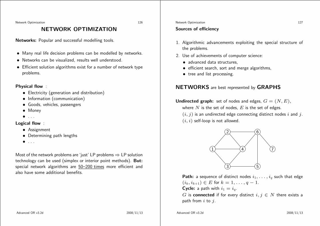
Network Optimization 126
NETWORK OPTIMIZATION
Networks: Popular and successful modelling tools.
• Many real life decision problems can be modelled by networks.
• Networks can be visualized, results well understood.
• Efficient solution algorithms exist for a number of network type
problems.
Physical flow :
• Electricity (generation and distribution)
• Information (communication)
• Goods, vehicles, passengers
• Money
• . . .
Logical flow :
• Assignment
• Determining path lengths
• . . .
Most of the network problems are ‘just’ LP problems ⇒ LP solution
technology can be used (simplex or interior point methods). But:
special network algorithms are 50–200 times more efficient and
also have some additional benefits.
Advanced OR v3.2d 2008/11/13
Network Optimization 127
Sources of efficiency
1. Algorithmic advancements exploiting the special structure of
the problems.
2. Use of achievements of computer science:
• advanced data structures,
• efficient search, sort and merge algorithms,
• tree and list processing.
NETWORKS are best represented by GRAPHS
Undirected graph: set of nodes and edges, G = (N, E),
where N is the set of nodes, E is the set of edges.
(i, j) is an undirected edge connecting distinct nodes i and j.
(i, i) self-loop is not allowed.
2 6
1 4 7
3 5
Path: a sequence of distinct nodes i1, . . . , iq such that edge
(ik, ik+1) ∈ E for k = 1, . . . , q − 1.
Cycle: a path with i1 = iq.
G is connected if for every distinct i, j ∈ N there exists a
path from i to j.
Advanced OR v3.2d 2008/11/13
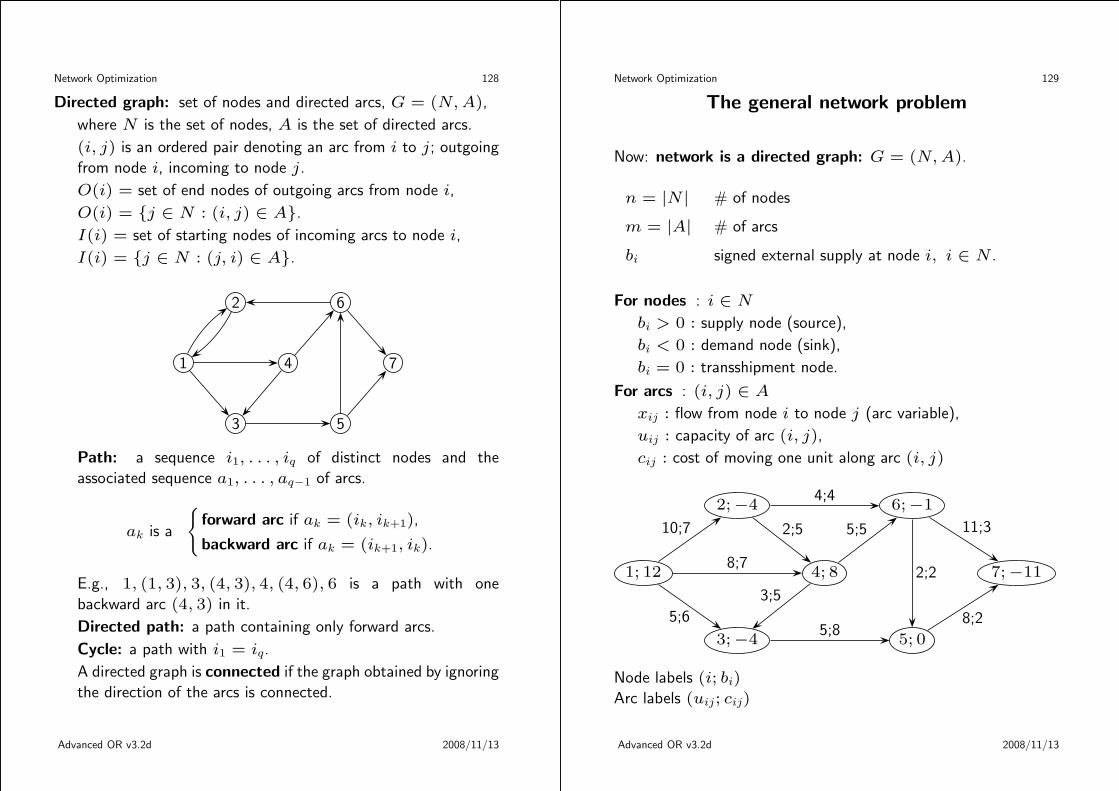
Network Optimization 128
Directed graph: set of nodes and directed arcs, G = (N, A),
where N is the set of nodes, A is the set of directed arcs.
(i, j) is an ordered pair denoting an arc from i to j; outgoing
from node i, incoming to node j.
O(i) = set of end nodes of outgoing arcs from node i,
O(i) = {j ∈ N : (i, j) ∈ A}.
I(i) = set of starting nodes of incoming arcs to node i,
I(i) = {j ∈ N : (j, i) ∈ A}.
2 6
1 4 7
3 5
Path: a sequence i1, . . . , iq of distinct nodes and the
associated sequence a1, . . . , aq−1 of arcs.
ak is a
{
forward arc if ak = (ik, ik+1),
backward arc if ak = (ik+1, ik).
E.g., 1, (1, 3), 3, (4, 3), 4, (4, 6), 6 is a path with one
backward arc (4, 3) in it.
Directed path: a path containing only forward arcs.
Cycle: a path with i1 = iq.
A directed graph is connected if the graph obtained by ignoring
the direction of the arcs is connected.
Advanced OR v3.2d 2008/11/13
Network Optimization 129
The general network problem
Now: network is a directed graph: G = (N, A).
n = |N | # of nodes
m = |A| # of arcs
bi signed external supply at node i, i ∈ N .
For nodes : i ∈ N
bi > 0 : supply node (source),
bi < 0 : demand node (sink),
bi = 0 : transshipment node.
For arcs : (i, j) ∈ A
xij : flow from node i to node j (arc variable),
uij : capacity of arc (i, j),
cij : cost of moving one unit along arc (i, j)
2;−4 6;−1
1; 12 4; 8 7;−11
3;−4 5; 0
10;7
5;6
8;7
2;5
3;5
4;4
5;5
5;8
2;2
11;3
8;2
Node labels (i; bi)
Arc labels (uij; cij)
Advanced OR v3.2d 2008/11/13

Network Optimization 130
Formal statement of the problem
Constraints :
Conservation of flow
bi +∑
j∈I(i)
xji =∑
j∈O(i)
xij, ∀i ∈ N
Bounds on flows
0 ≤ xij ≤ uij, ∀(i, j) ∈ A
Objective :
min∑
(i,j)∈A
cijxij
Advanced OR v3.2d 2008/11/13
Network Optimization 131
Minimal cost network flow (MCNF) problem
min∑
(i,j)∈A
cijxij
subject to∑
j∈O(i)
xij −∑
j∈I(i)
xji = bi, ∀i ∈ N
0 ≤ xij ≤ uij, ∀(i, j) ∈ A
This is an LP problem of the form:
min cTx
s.t. Ax = b
0 ≤ x ≤ u
Here, A is an arc-node incidence matrix
Column representing arc (i, j):
+1 in position i (from)−1 in position j (to)
0 elsewhere
Necessary condition for the feasibility of the problem:∑
i∈N
bi = 0.
Advanced OR v3.2d 2008/11/13

Net
wor
kO
ptim
izat
ion
132
MCN
F:m
atr
ixfo
rmofth
eexa
mple
Ar
cs
Nodes
(1,2)
(1,3)
(1,4)
(2,4)
(2,6)
(3,5)
(4,3)
(4,6)
(5,7)
(6,5)
(6,7)
b i
11
11
12
2−
11
1−
4
3−
11
−1
−4
4−
1−
11
18
5−
11
−1
0
6−
1−
11
1−
1
7−
1−
1−
11
uij
10
58
24
53
58
211
cij
76
75
48
55
22
3
Adva
nce
dO
Rv3
.2d
2008/11/13 Network Optimization 133
Integrality property: If all bi and uij are integer then
every basic feasible solution (including optimal BFS) is
integer valued (because A satisfies property K).
Additional properties of MCNF
• If all data (including cij) are integer then both primal and dual
BFSs are integer.
• Every basis B to A is triangular ⇒ no need for explicit B−1.
• The subgraph corresponding to B is a tree T .
• Simplex operations involving B−1 are performed using the tree
representation.
• Most of the (or the entire) algorithm can work with integer
arithmetic.
Advanced OR v3.2d 2008/11/13

Network Optimization 134
Transportation problem
Transporting a single commodity.
m # of supply nodesn # of demand nodessi supply at node i, i = 1, . . . , mdj demand at node j, j = 1, . . . , ncij cost of transporting one unit
from supply node i to demand node j,xij (unknown) quantity transported from node i to node j.
Assumption:
Total supply is equal to total demand:
m∑
i=1
si =n∑
j=1
dj.
Objective:
To satisfy every demand with the least possible total cost.
minm∑
i=1
n∑
j=1
cijxij
subject to
m∑
i=1
xij = dj, j = 1, . . . , n
n∑
j=1
xij = si, i = 1, . . . , m
m∑
i=1
si =
n∑
j=1
dj
xij ≥ 0, ∀(i, j)
Advanced OR v3.2d 2008/11/13
Network Optimization 135
Capacitated transportation problem: all the above plus bounds
on arc variables:
0 ≤ xij ≤ uij, for some or all (i, j)
The equivalent MCNF form (example):
1 =⇒ d1
s1 =⇒ 1 2 =⇒ d2
s2 =⇒ 2 3 =⇒ d3
4 =⇒ d4
bi > 0 bi < 0
Bipartite graph: Nodes are divided into two groups (supply and
demand nodes, in this case); there is no connection between nodes
within a group.
Advanced OR v3.2d 2008/11/13

Network Optimization 136
Transshipment problem
It is a generalization of the transportation problem. It is assumed
that a given commodity is produced at different sources. It is then
delivered to intermediate storages which supply the customers.
6
1
4 7
2
5 8
3
9
bi > 0 bi = 0 bi < 0
The diagram clearly shows how this transshipment problem can be
formulated as an MCNF problem with 9 nodes and 14 arcs.
Arc capacities can also be imposed leading to the capacitated
transshipment problem.
Advanced OR v3.2d 2008/11/13
Network Optimization 137
Assignment problem
m # of assignees (workers, vehicles, machines)
m # of tasks
Assumptions:
Each assignee must be assigned to exactly one task.
Each task is to be performed by one assignee.
cij cost associated with assignee i performing task j.
Objective:
Find an optimal (min cost) assignment.
xij =
{
1, if assignee i ⇒ task j
0, otherwise.
min
m∑
i=1
m∑
j=1
cijxij
subject tom∑
i=1
xij = 1, j = 1, . . . , m
m∑
j=1
xij = 1, i = 1, . . . , m
xij ∈ {0, 1}, ∀(i, j)
Advanced OR v3.2d 2008/11/13

Network Optimization 138
The assignment problem is a special case of the transportation
problem, and thus the MCNF problem, with the following
interpretation.
Employee Job
1 1
2 2
3 3
bi = 1 bi = −1
Advanced OR v3.2d 2008/11/13
Network Optimization 139
Maximum flow problem
Given a directed graph G = (N, A) with two special nodes
s : source node,
t : sink node.
Flow on arc (i, j) is bounded: 0 ≤ xij ≤ uij.
N.B. Some (but not all) uij can be +∞.
Find the maximum possible flow from source to sink, subject
to the usual constraints (conservation of flow, arc capacities,
nonnegativity of the flow) with zero external supply at all nodes
different from s and t.
max bs
subject to
Ax = b
bt = −bs
bi = 0, i 6= s, t
0 ≤ xij ≤ uij, ∀(i, j) ∈ A.
Note: bs is a variable now (so is bt).
Advanced OR v3.2d 2008/11/13

Network Optimization 140
Reformulation of maximum flow as a minimum cost network flow
problem:
Let cij = 0 for all (i, j).
Connect sink and source with an arc (t, s) of infinite capacity and
a negative (say, −1) cost.
Let A = A ∪ {(t, s)} and let xts denote the corresponding arc
variable.
If we minimize∑
(i,j)∈A
cijxij (which is equal to −xts) then the
negative cost coefficient of arc (t, s) will force the flow through
t (and also s) to increase as much as possible. Other constraints
are the same as in the maxflow formulation.
... ...
s ... ... t
... ...
cts = −1, uts = +∞
Advanced OR v3.2d 2008/11/13
Network Optimization 141
Shortest path problem
Given a directed graph G = (N, A), |N | = n, |A| = m.
cij is the length (or cost) of traversing arc (i, j) for each (i, j) ∈A.
Length of a path is the sum of cij along the path.
Shortest path from i to k: one with minimum length among all
possible paths from i to k.
Instead of finding the shortest path between two nodes in A, we
can determine the shortest path from all nodes to a designated
node (say, n) in the network.
Assumptions:
• From every i 6= n there exists a path to n.
• O(n) = ∅ (no outgoing arc from n).
2 6
1 4 7
3 5
3
2
8
5
6
2
3
9
3
9
5
Advanced OR v3.2d 2008/11/13

Network Optimization 142
MCNF formulation:
Every node i 6= n is given a unit (+1) supply, node n has a
demand −(n − 1).
Arc capacities are infinite.
Formally, uij = ∞, ∀(i, j) ∈ A,
bi = 1, i 6= n,
bn = −(n − 1).
The MCNF problem to be solved is:
min∑
(i,j)∈A
cijxij
subject to∑
j∈O(i)
xij −∑
j∈I(i)
xji = bi, ∀i ∈ N
xij ≥ 0, ∀(i, j) ∈ A
The arcs in the optimal basis of this problem form a tree rooted
at node n. In this tree there is a unique path from every node
i 6= n to the root and this is the shortest path from i to n.
Advanced OR v3.2d 2008/11/13
Logic and MIP 143
LOGIC CONSTRAINTS AND (M)IP
Indicator variables
Sometimes it is important to indicate that a variable is in a certain
state, like x > 0 (see fixed charge problem). It can be achieved
by the introduction of a 0/1 variable δ. We actually want to
represent the condition
x > 0 → δ = 1, (72)
which reads ‘x greater than zero implies δ = 1’. Assuming that
x has a known upper bound, S, (72) can be expressed as
x − Sδ ≤ 0, (73)
because for any x > 0 this constraint can only be satisfied if the
maximum possible value of x, S, is subtracted from it. As such,
x > 0 forces δ to be 1.
Advanced OR v3.2d 2008/11/13

Logic and MIP 144
We may also wish to impose the condition
x = 0 → δ = 0, (74)
which is equivalent to
δ = 1 → x > 0 (75)
Combining (72) and (74) (or (75)) we get ‘δ = 1 if and only if
x > 0’ or
δ = 1 ↔ x > 0. (76)
Representing (75) or (76) by a constraint is not possible. If a
tolerance level ǫ > 0 is given to x for being different from zero
then (75) can be rewritten as
δ = 1 → x ≥ ǫ (77)
which can be imposed by the constraint
x − ǫδ ≥ 0.
Summarizing the above, if we want to express x is positive if and
only if δ = 1 (see (76)) it can be achieved by the following two
inequalities and an indicator variable δ ∈ {0, 1}:
x − Sδ ≤ 0
and
x − ǫδ ≥ 0.
Advanced OR v3.2d 2008/11/13
Logic and MIP 145
Example 19 (The fixed charge problem) Let x represent the
quantity of a product with unit production cost of c1. If the product
is manufactured at all, there is a setup cost of c2 associated with
it. Thus, the cost of producing x units is
z =
{
0, if x = 0
c1x + c2, if x > 0.
Clearly, z is not linear, and not even continuous, see diagram.
x
z
c2
0
slope= c1
We can introduce indicator variable δ such that x > 0 → δ = 1.
Now the total cost z can be expressed as
z = c1x + c2δ,
i.e., by the introduction of a 0/1 variable δ and an extra constraint
for the logical condition x > 0 → δ = 1, we could model the
situation as a MIP problem. Note, if cost is minimized condition
x = 0 → δ = 0 need not be modelled.
Advanced OR v3.2d 2008/11/13

Logic and MIP 146
Consider inequalityn∑
j=1
ajxj ≤ b. (78)
We can use an indicator variable to show whether it is satisfied or
not. More precisely, we want to model the following:
δ = 1 →n∑
j=1
ajxj − b ≤ 0. (79)
Let S denote the largest value the expression∑
ajxj − b can
take. Now (78) can be imposed by
n∑
j=1
ajxj − b ≤ S(1− δ), or
placing the variables on the LHS:
n∑
j=1
ajxj + Sδ ≤ b + S. (80)
It is easy to see that if δ = 1 the desired relation is enforced and if
δ = 0 no additional constraint is imposed as∑n
j=1 ajxj−b ≤ S
always holds by the definition of S.
Advanced OR v3.2d 2008/11/13
Logic and MIP 147
To model the reverse of (79), namely,
n∑
j=1
ajxj − b ≤ 0 → δ = 1,
we consider the equivalent
δ = 0 →n∑
j=1
ajxj − b > 0 (81)
which can be modeled only if we allow for a tolerance ǫ > 0 as in
(77):
n∑
j=1
ajxj ≥ b + ǫ. Now we can rewrite (81) as
δ = 0 → −n∑
j=1
ajxj + b + ǫ ≤ 0,
which can be represented by the constraint
n∑
j=1
ajxj − (s − ǫ)δ ≥ b + ǫ, (82)
where s is a lower bound for expression∑
j ajxj − b.
To verify this expression, first substitute δ = 0 which gives the
desired relation, next take δ = 1 and observe that (82) now
reduces to∑
j ajxj − b ≥ s which always holds by the definition
of s.
Advanced OR v3.2d 2008/11/13

Logic and MIP 148
To monitor whether constraint
n∑
j=1
ajxj ≥ b (83)
is satisfied or not an indicator variable δ should be introduced. If
(83) is transformed into a ‘≤’ the developed technique (79)–(82)
can be used. First, we express
δ = 1 →n∑
j=1
ajxj ≥ b (84)
(or the equivalent δ = 1 → −∑
j ajxj ≤ −b). If s and S
denote the smallest and largest values expression∑
j ajxj − b
can take, (84) is equivalent to −∑
j ajxj + b ≤ −s(1 − δ), or
n∑
j=1
ajxj + sδ ≥ b + s. (85)
Next, to express
n∑
j=1
ajxj ≥ b → δ = 1,
the quoted procedure results in
n∑
j=1
ajxj − (S + ǫ)δ ≤ b − ǫ. (86)
Advanced OR v3.2d 2008/11/13
Logic and MIP 149
Example 20 Use a 0/1 variable to indicate whether or not
constraint
4x1 + x2 ≤ 2
is satisfied, where 0 ≤ x1 ≤ 1 and 0 ≤ x2 ≤ 1 are continuous
variables. The two relations we want to impose are
δ = 1 → 4x1 + x2 ≤ 2 (87)
4x1 + x2 ≤ 2 → δ = 1. (88)
First, determining s and S for 4x1 + x2 − 2, we obtain s =
0 + 0 − 2 = −2, and S = 4 + 1 − 2 = 3. Applying (80), (87)
can be expressed as
4x1 + x2 + 3δ ≤ 5 (being 2 + 3).
Applying (82) with ǫ = 0.1, (88) results in
4x1 + x2 + 2.1δ ≥ 2.1
Advanced OR v3.2d 2008/11/13

Logic and MIP 150
What remains to be investigated is how an indicator variable can
be used to force an equality constraint
∑
j
ajxj = b
to be satisfied or violated. Equality means ≤ and ≥ hold
simultaneously. On the other hand, 6= means only one of the
inequalities holds.
To express δ = 1 →∑
j ajxj = b we can use δ = 1 to indicate
that both inequalities hold simultaneously, i.e., we apply this δ in
both (80) and (85).
With δ = 0 we want to force one of the derived ≤ and ≥constraints to be violated. To achieve it, δ′, δ′′ ∈ {0, 1} are
introduced and used to impose (82) and (86):
n∑
j=1
ajxj − (s − ǫ)δ′ ≥ b + ǫ,
n∑
j=1
ajxj − (S + ǫ)δ′′ ≤ b − ǫ.
One more constraint is to be added to force the required condition
δ′ + δ′′ − δ ≤ 1.
Advanced OR v3.2d 2008/11/13
Logic and MIP 151
Logical conditions and 0/1 variables
Many different types of logical conditions can be modelled by 0/1
variables (examples to come).
Notation
Propositions: P, Q, R, . . . , X, Y .
Example: P can stand for x > 0.
Connectives:
∨ inclusive ‘or’
∧ ‘and’
¬ ‘not’
→ ‘implies’ (or ‘if . . . then . . . ’)
↔ ‘if and only if’ (‘iff’)
The precedence order of the connectives from highest to lowest is
‘¬’, ‘∧’, ‘∨’ and ‘→’.
Example 21 If Xi represents proposition ‘Ingredient i is in the
blend’, i ∈ {A, B, C}, then proposition ‘If ingredient A is in the
blend then ingredient B or C (or both) must also be in the blend’
can be expressed by XA → (XB ∨ XC) which is equivalent to
(XA → XB) ∨ (XA → XC).
Advanced OR v3.2d 2008/11/13

Logic and MIP 152
Correspondence can be established between propositions and
indicator variables. If δi is a 0/1 indicator variable then Xi
can stand for the proposition δi = 1. In this way the following
propositions and constraints are equivalent:
X1 ∨ X2 ↔ δ1 + δ2 ≥ 1
X1 ∧ X2 ↔ δ1 = 1, δ2 = 1
¬X1 ↔ δ1 = 0
X1 → X2 ↔ δ1 − δ2 ≤ 0
X1 ↔ X2 ↔ δ1 − δ2 = 0
Example 22 Express the logical relationship of Example 21 with
constraints containing 0/1 variables. Reminder: Xi represents
proposition ‘Ingredient i is in the blend’, i ∈ {A, B, C}. We
are interested in proposition ‘If ingredient A is in the blend then
ingredient B or C (or both) must also be in the blend’, or
XA → (XB ∨ XC).
Solution: Let indicator variables δi correspond to Xi, i ∈{A, B, C}. Since XB ∨ XC can be expressed as δB + δC ≥ 1,
we want to impose δA = 1 → δB+δC ≥ 1. This is the situation
shown in (84). Now we have to compute s for δB + δC −1 which
is −1. The required implication can be ensured by (85) which
gives δB + δC + (−1)δA ≥ 1 − 1 or
−δB − δC + δA ≤ 0.
If there are other constraints in the model we have to add the
above variables and the constraint to them.
Advanced OR v3.2d 2008/11/13
Logic and MIP 153
Utilizing equivalent formulations
The following logical condition is often part of an optimization
model (assuming all δs are indicator variables):
δ1 = 1 ∨ δ2 = 1 ∨ · · · ∨ δn = 1 → δ = 1. (89)
This condition can be imposed by the constraint
δ1 + δ2 + · · · + δn − nδ ≤ 0. (90)
(89) can also be written in an equivalent form:
δ = 0 → δ1 = 0 ∧ δ2 = 0 ∧ · · · ∧ δn = 0. (91)
(91) can be imposed by n constraints:
δ1 − δ ≤ 0
... (92)
δn − δ ≤ 0.
If all other LP constraints are similar to the ones in (92) then AT
satisfies property K. Taking the dual of the problem, we have a
totally unimodular matrix that guarantees the all integer solution
of the problem. Therefore, it is sufficient to solve the LP relaxation
of the problem which will be integer. In other words, in this way
constraints define the convex hull of integer solutions.
If not all LP constraints are in the form of (92) then this formulation
is still preferred to (90) because it results in a tighter formulation
of the problem.
Advanced OR v3.2d 2008/11/13

Logic and MIP 154
Example 23 (Tighter formulation) We can illustrate why a
series of constraints like (92) is preferable to a single constraint
(90). While the two formulations are equivalent in logical and
also in IP sense (actually, (90) is the sum of constraints in (92))
they are not equivalent in an LP sense. By adding together
constraints in LP we generally get a larger feasible region, i.e., a
looser formulation.
E.g., for n ≥ 3 the solution
δ1 =1
2, δ2 = δ3 =
1
4, δ =
1
n, all other δi = 0
satisfies (90) but does not satisfy (92).
This example shows that (92) is more effective in eliminating
useless fractional solutions.
When linking a continuous x and an indicator δ variable in a
constraint we used some upper bound on x. For instance,
x > 0 → δ = 1,
was represented by the constraint
x − Sδ ≤ 0
where S is a true upper bound on x. In the light of the preceding
discussion, it is quite important to keep S as small as possible and
thus tightening the LP relaxation. It is usually the owner of the
model who can determine the smallest realistic value for S.
Advanced OR v3.2d 2008/11/13
Logic and MIP 155
Disjunctive Constraints in LP
In several real-life problems we do not require all constraints to
hold but at least one subset of constraints. This can be stated
as
R1 ∨ R2 ∨ · · · ∨ RM, (93)
where Ri stands for the proposition ‘Constraints in subset i
are satisfied’, 1 ≤ i ≤ M . (93) is known as disjunction of
constraints.
Introduce indicator variables δi to indicate whether constraints in
Ri are satisfied. To fulfil (93), we impose
δi = 1 → Ri
for all subsets. Keeping in mind that Ri represents a (sub)set
of constraints (that can be of any type), we have to apply
the techniques of section ‘Logic Constraints and (M)IP’ to each
constraint, all with the single indicator variable δi in the subset.
Having done it for all 1 ≤ i ≤ M , we can impose condition (93)
by the constraint
δ1 + δ2 + · · · + δM ≥ 1.
If the condition to be modelled is ‘at least k subsets have to be
satisfied out of M ’ the we can write
δ1 + δ2 + · · · + δM ≥ k.
Advanced OR v3.2d 2008/11/13

Logic and MIP 156
Condition ‘at most k of the subsets must be satisfied’ can
also be modelled. Now, indicator variables are used to express
conditions
Ri → δi = 1.
This, again, involves handling all constraints individually in Ri
according to their relation (≤, =, ≥) and then imposing
δ1 + δ2 + · · · + δM ≤ k.
Interesting to note that the connective ‘∧’ (‘and’) is usually not
needed explicitly in LP since a conjunction of constraints simply
involves a series of constraints holding simultaneously.
Example 24 (Limiting the number of active variables) In the
standard LP problem there are no more than m variables different
from zero in an optimal solution. Sometimes this number has to
be further restricted to k < m for some (usually technological)
reasons. Even if the original problem was an LP this restriction
can be modelled by IP. We associate an indicator variable δj with
each continuous variable xj to indicate the condition xj > 0 →δj = 1. As shown earlier, this can be imposed by the constraint
xj −Sjδj ≤ 0, where Sj is an upper bound on xj. Now, we can
impose the condition that no more than k continuous xj variables
can be nonzero in any feasible solution:
δ1 + δ2 + · · · + δn ≤ k.
Some typical situations for this type of a condition are limiting the
number of (i) different stocks in a portfolio, (ii) ingredients in a
blend, (iii) cutting knifes in cutting stock problems.
Advanced OR v3.2d 2008/11/13
Logic and MIP 157
Example 25 (Discrete capacity expansion) If a constraint
represents a capacity limitation it may not be possible to expand it
continuously but rather in steps, i.e., by installing a new machine
or building a new storage.
Suppose the initial RHS value of the constraint is b0 which may
be successively increased to b1 < b2 < · · · < bt. The actual LP
constraint will be one of the following:
n∑
j=1
ajxj ≤ bi, i = 0, 1, . . . , t,
where i = 0 represents the original constraint. The expansions
incur costs 0 < c1 < c2 < · · · < ct, respectively. To model the
situation, we introduce indicator variables δi, i = 0, 1, . . . , t to
represent the successive possible RHS values. We then have
n∑
j=1
ajxj − b0δ0 − b1δ1 − · · · − btδt ≤ 0
δ0 + δ1 + · · · + δt = 1, (94)
and the following expression is added to the objective function
c1δ1 + c2δ2 + · · · + ctδt.
(94) ensures that exactly one of the alternatives is selected. It
is interesting to note that in the LP relaxation (0/1 variables
δ0, δ1, . . . , δt are relaxed to 0 ≤ δi ≤ 1, i = 0, . . . , t) the
integrality requirement is automatically satisfied.
Advanced OR v3.2d 2008/11/13

Logic and MIP 158
Example 26 (Maximax objectives) (Not to be mistaken for
minimax.) Assume we are given some linear expressions
n∑
j=1
aijxj, i = 1, . . . , m,
that are evaluated for different sets of xj values. We may be
interested in the following problem. Find x1, . . . , xn such that
max
maximumi
n∑
j=1
aijxj
subject to conventional LP constraints.
While this problem shows similarities to the minimax objective
(that can be modelled by LP), we have to treat it as a case of a
disjunctive constraint and use IP. Introducing a continuous variable
z, the model can be expressed as
max z
subject to
n∑
j=1
a1jxj − z = 0
or . . .
or
n∑
j=1
amjxj − z = 0
and the technique of handling disjunctive constraints can be used.
Advanced OR v3.2d 2008/11/13
MIP 159
State-of-the-art in MIP
Currently, there is no single best general purpose (M)IP solver.
The most widely used solution algorithms are based on the Branch
and Bound principle. First LP relaxation is solved by IPM or the
SM and re-optimizations are done by the dual SM.
As mentioned earlier, MIP is sensitive to the number of integer
variables. E.g., if there are 100 0/1 variables in a model the
number of all possible combinations of them is 2100 ≈ 1030. A
B&B method will test all of them (mostly implicitly). Depending
on the branching strategy, the computational effort can vary
enormously. Defining a good strategy often lies in the hands of
the model owner who knows which are the ‘important’ integer
variables that are useful to branch on.
Model formulation also heavily influences the efficiency of
solution. Tighter formulations are more easily solved than less tight
ones. Some algorithmic procedures can help tighten constraints
but the modeller can do the most in this respect.
There are very few general purpose MIP solvers available
(commercial or academic). They are all built around a state-
of-the-art LP solver. Dual SM is a ‘must’ for MIP since a very
large proportion of the solution time is spent on re-optimization.
Problems with several hundreds of 0/1 (and many continuous)
variables and tens of thousands of constraints can be solved if
properly formulated. The variation is big, anything can happen
from efficient solution to unsolvability. However, skilled users have
good chances to solve large real-life MIP problems.
Advanced OR v3.2d 2008/11/13

Modelling Languages 160
MODELLING LANGUAGES
Need for modelling languages
Real-world LP and (M)IP problems tend to be very large. They
have to be formulated, edited, verified and maintained. All these
functions call for a model management system. Optimization
modelling languages have been created to make the above activities
possible in a convenient and efficient way. They also serve as a
documentation of the work done.
A key requirement is to allow formulation in a similar way as
humans naturally do it. This enables better understanding of the
model.
Several optimization modelling languages have been developed and
implemented since the early 1990s. They all share certain common
features. Here are some of the most important ones.
• Model building is supported by a model editor.
• Separation of model and data.
• Variables and constraints are identified by meaningful names.
• Sophisticated indexing of variables is possible.
• Variables can be placed on both sides of constraints.
• Algebraic expressions can be used for defining constraints.
• Logical relationships can be defined.
• Data can be imported.
• Macros can be defined for repetitive parts of the model.
• Comments can be inserted anywhere in the model description.
Advanced OR v3.2d 2008/11/13
Modelling Languages 161
Typical structure of a model file
Definition Part:
TITLE Name of the problem
INDEX Dimensions of the problem
DATA Scalars, vectors, data files
VARIABLES Vector variables
MACROS Macros for repetitive parts
Model Part:
MODEL
MAX or MIN The objective function.
SUBJECT TO The constraints.
BOUNDS Individual bounds on variables.
FREE Free variables.
INTEGER Integer variables.
BINARY Binary variables.
END
The output of the model editor is a file that constitutes the input
of an LP/MIP solver. Several formats for the output can be
chosen. The most important one is the widely used industrial
standard MPS input format.
Advanced OR v3.2d 2008/11/13

Modelling Languages 162
Example of MPS format
NAME Return maximization (simplified)
ROWS
N Return
L Row1
L Row2
L Row3
L Row4
COLUMNS
Var1 Return 5.4000 Row1 0.5000
Var1 Row2 0.2500 Row3 -1.0000
Var1 Row4 1.0000
Var2 Return 7.3000 Row2 0.5000
Var2 Row3 1.0000
Var3 Return 12.9600 Row1 0.6000
Var3 Row2 0.6000
Var4 Return -6.0000 Row1 -1.0000
Var5 Return -9.0000 Row2 -1.0000
RHS
Constr Return 800.0000 Row1 80.0000
Constr Row2 40.0000 Row4 150.0000
RANGES
Range1 Row4 50.0000
BOUNDS
UP Bound1 Var4 20.0000
UP Bound1 Var5 10.0000
ENDATA
Note, the fields have fixed positions and names cannot be longer
than 8 characters. The direction of optimization (min or max)
cannot be defined in MPS format.
Advanced OR v3.2d 2008/11/13
Modelling Languages 163
The following example highlights the use of the different
components of a modelling language.
Aggregate production planning
A company wants to
• distribute production capacity among products,
• determine production and inventory levels in order to meet
demand for each product
in every month while maximizing its profit.
The company has three products.
Planning is done for twelve months.
Prices, demands, production capacity and cost are fixed for the
whole period.
The decision variables are monthly production, sales and inventory.
Advanced OR v3.2d 2008/11/13

Modelling Languages 164
TITLE
Production Planning;
INDEX
product = 1..3;
month = {Jan,Feb,Mar,Apr,May,Jun,
Jul,Aug,Sep,Oct,Nov,Dec};
DATA
Price[product] := (99.00,240.00,750.00);
Demand[month,product] := DATAFILE(demand.dat);
ProdCapacity[product] := (1000.0,550.0,220.0);
ProdCost[product] := (55.60,176.40,585.30);
InvCost := 6.55; \\ Inventory unit cost
VARIABLES
Inventory[product,month] -> Invt \\ Short name
Prod[product,month] \\ Production
Sales[product,month] -> Sale \\ Short name
MACRO
Revenues := SUM(product,month: Price * Sales);
TotalCost := SUM(product,month: InvCost * Inventory
+ ProdCost * Prod);
MODEL
MAX Profit = Revenues - TotalCost;
SUBJECT TO
InventoryBalance[product,month]: \\ Constraint name
Inventory[month] = Inventory[month-1] + Prod - Sales;
BOUNDS
Sales < Demand;
Prod < ProdCapacity;
Inventory[product,month=Jan..Nov] < 8000;
Inventory[product,Dec] = 1800;
END
If short names are given they are used in the generated MPS file
(where names are limited to 8 characters).
Advanced OR v3.2d 2008/11/13
Modelling Languages 165
The model editor will generate decision variables for Inventory,Production and Sales for each product for each month of theyear (108 variables). Using the short names, the finally generatedvariable names as used in the MPS format may look as follows:
Invt1Jan Invt2Jan Invt3Jan
Invt1Feb Invt2Feb Invt3Feb
... ... ...
Invt1Dec Invt2Dec Invt3Dec
Prod1Jan Prod2Jan Prod3Jan
... ... ...
Prod1Dec Prod2Dec Prod3Dec
Sale1Jan Sale2Jan Sale3Jan
... ... ...
Sale1Dec Sale2Dec Sale3Dec
There will be an inventory constraint generated for each product
for months Feb to Dec, altogether 33 of them. Starting inventory
is assumed to be zero. Inventory levels are further restricted by
individual bounds.
Other bounds restrict sales (no more can be sold than the demand
is) and production (production capacity cannot be exceeded).
While the above model as described in this language is quite
understandable, the corresponding MPS file is much less intuitive.
In case of large scale problems the advantages of a modelling
system are even more obvious. Actually, such problems simply
cannot be handled without a proper modelling system.
Advanced OR v3.2d 2008/11/13